Crosstalk-insensitive method for simultaneously coupling multiple pairs of resonators

Abstract

In a circuit consisting of two or more resonators, the inter-cavity crosstalk is inevitable, which could create some problems, such as degrading the performance of quantum operations and the fidelity of various quantum states. The focus of this work is to propose a crosstalk-insensitive method for simultaneously coupling multiple pairs of resonators, which is important in large-scale quantum information processing and communication in a network consisting of resonators or cavities. In this work, we consider $2N$ resonators of different frequencies, which are coupled to a three-level quantum system (qutrit). By applying a strong pulse to the coupler qutrit, we show that an effective Hamiltonian can be constructed for simultaneously coupling multiple pairs of resonators. The main advantage of this proposal is that the effect of inter-resonator crosstalks is greatly suppressed by using resonators of different frequencies. In addition, by employing the qutrit-resonator dispersive interaction, the intermediate higher-energy level of the qutrit is virtually excited and thus decoherence from this level is suppressed. This effective Hamiltonian can be applied to implement quantum operations with photonic qubits distributed in different resonators. As one application of this Hamiltonian, we show how to simultaneously generate multiple EPR pairs of photonic qubits distributed in $2N$ resonators. Numerical simulations show that it is feasible to prepare two high-fidelity EPR photonic pairs using a setup of four one-dimensional transmission line resonators coupled to a superconducting flux qutrit with current circuit QED technology.

I. INTRODUCTION

Circuit Quantum Electrodynamics (QED), consisting of microwave resonators and superconducting qubits, has quickly developed in the last decade and is considered one of the most promising platforms for quantum information processing (QIP) (for reviews, see [1-4]). Superconducting qubits are very important in solid-state quantum computation and QIP, due to the controllability of their level spacings, the scalability of circuits, and the improvement of coherence times [5-14]. High-quality-factor microwave resonators have also drawn much attention because they have many applications in QIP; for example, they can be used as quantum data buses [15-18] and quantum memories [19,20]. A superconducting coplanar waveguide resonator with a (loaded) quality factor $Q=10^{6}$ [21,22] or with an internal quality factor above $10^{7}$ [23] was previously reported. Superconducting microwave resonators with a loaded quality factor $Q=3.5\times 10^{7}$ have been recently demonstrated in experiments [24], for which the single-photon lifetime can reach near one millisecond, while the cavity mode remains strong-coupled with a superconducting qubit. The strong or ultrastrong coupling between a superconducting qubit and a microwave cavity has been experimentally observed [18,25-27]. Moreover, quantum phenomena, such as squeezing or multiphoton quantum Rabi oscillations in the ultrastrong coupling regimes, have been theoretically investigated [28,29].

As this is relevant to this work, here we provide a brief review on the production and manipulation of quantum states of microwave photons in circuit QED. For convenience, the term cavity and resonator will be used interchangeably. During the past years, a number of theoretical works [30-35] have been done on the preparation of Fock states, coherent states, squeezed states, Schrodinger cat states and an arbitrary superposition of Fock states of a single superconducting cavity. Experimentally, the creation of a Fock state or a superposition of Fock states of a single superconducting cavity has been reported [17,36,37]. In recent years, attention has shifted to larger systems involving two or more cavities. Based on circuit QED, many theoretical proposals have been presented for implementing quantum state synthesis of photons in two resonators $[38,39$], generating entangled photon Fock states of two resonators [40,41], creating photon NOON states of two resonators [38,39,42,43], and preparing entangled photon Fock states or entangled coherent states of more than two cavities [44-46]. In addition, schemes for realizing two-qubit or multi-qubit quantum gates with microwave photons distributed in different cavities have been proposed [47,48]. Experimentally, the creation of photon NOON states of two resonators has been reported [49], and the coherent transfer of microwave photons between three resonators interconnected by two phase qubits has also been demonstrated [50]. All these works are fundamental and important, and open new avenues to use microwave photons as resource for quantum computation and communication.

In a circuit consisting of two or more resonators, the inter-cavity crosstalk is inevitable, which could create some problems, such as degrading the performance of quantum operations and the fidelity of various quantum states. Let us consider a two-cavity system, for which the inter-cavity crosstalk is described by the Hamitonian $H=g(e^{i\Delta t}ab^{+}+e^{-i\Delta t}a^{+}b)$, where $g$ is the inter-cavity crosstalk strength between the two cavities, $\Delta$ is the detuning between the frequencies of the two cavities, and $a$ ($b$) is the photon annihilation operator of one (the other) cavity. From the form of the Hamiltonian $H$, it can be seen that the effect of the cavity-cavity crosstalk depends on the ratio of $\alpha=\Delta/g$, which increases as $\alpha$ decreases. In other words, the effect of the cavity crosstalk is strongest for $\Delta=0$ (i.e., when the two cavities have the same frequency), while it can be reduced by increasing $\alpha$ (e.g., increasing the detuning $\Delta$ for a given $g$). The discussion here gives a hint on how to reduce the effect of the inter-cavity crosstalk. Namely, in order to reduce the effect of the inter-cavity crosstalk, one could employ cavities with different frequencies.

In this work, we focus on a physical system consisting of $2N$ resonators coupled to a three-level quantum system (qutrit). It is shown that by applying a strong pulse to the coupler qutrit, an effective Hamiltonian can be obtained for simultaneously coupling multiple pairs of resonators with different frequencies, which is insensitive to the inter-resonator crosstalk. This effective Hamiltonian can be applied to implement quantum operations with photonic qubits distributed in different resonators. The major advantage of this proposal is that the inter-resonator crosstalk is greatly reduced because of using different resonator frequencies. In addition, the intermediate higher-energy level of the qutrit is virtually excited due to the qutrit-resonator dispersive interaction, and thus decoherence from this level is greatly suppressed.

As one application of this constructed Hamiltonian, we show how to simultaneously generate multiple Einstein-Podolsky-Rosen (EPR) pairs [51] of photonic qubits distributed in $2N$ resonators. The prepared EPR pairs are particularly useful in quantum communication and QIP. As a specific experimental realization, we further discuss the possible experimental implementation of two EPR pairs of photonic qubits using a setup consisting of four one-dimensional transmission line resonators coupled to a superconducting flux qutrit. With realistic device and circuit parameters, numerical simulations show that the fidelity can reach $98.42\%$ for the joint state of two EPR pairs and is no less than $99.05\%$ for each EPR pair.

We note that previous works focused on the preparation of a single EPR pair in various physical systems, such as neutral Kaons [52], trapped ions [53,54], atoms interacting with a cavity mode [55-58], Bose-Einstein condensates [59-61], two harmonic oscillators in nonequilibrium open systems [62], center-of-mass motion of two massive objects [63], and superconducting qubits [15,64-66]. In stark contrast, ours is aimed at simultaneously generating multiple EPR pairs by using the constructed Hamiltonian, which is insensitive to the inter-resonator crosstalk.

This paper is organized as follows. In Sec. II, we derive the effective Hamiltonian governing the dynamics of $N$ pairs of cavities plus one three-level coupler qutrit. This Hamiltonian describes paired interactions between these cavities in parallel without interfering with each other. In Sec. III, we show in detail how to simultaneously prepare $N$ pairs of photonic qubits using this effective Hamiltonian. In Sec. IV, we discuss the possible experimental implementation of generating EPR states of two pairs of photonic qubits in circuit QED. In Sec. V, we summarize our results and discuss other possible applications of this physical process.

II. EFFECTIVE HAMILTONIAN

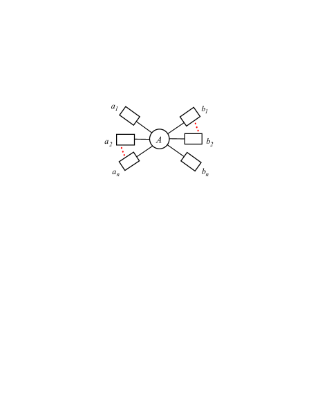
Figure 1: (color online) Diagram of a coupler qutrit $A$ (the circle at the center) and $2n$ coupled resonators. Each rectangle represents a resonator. The coupler qutrit $A$ can be an artificial atom, such as a quantum dot or a superconducting qutrit capacitively/inductively coupled to each resonator.

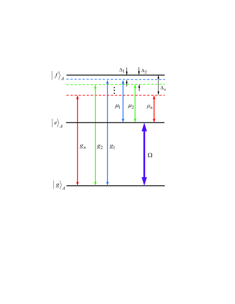
Figure 2: (Color online) Illustration of the qutrit-resonator dispersive interaction. The $\left|g\right\rangle$ $\leftrightarrow$ $\left|f\right\rangle$ transition of the qutrit is simultaneously coupled to the $n$ resonators ($a_{1},a_{2},...,a_{n}$), with coupling constants $g_{1},g_{2},...,g_{n}$ and detunings $\Delta_{1},\Delta_{2},...,\Delta_{n}$, respectively. The $\left|e\right\rangle$ $\leftrightarrow$ $\left|f\right\rangle$ transition of the qutrit is simultaneously coupled to the other $n$ resonators ($b_{1},b_{2},...,b_{n}$), with coupling constants $\mu_{1},\mu_{2},...,\mu_{n}$ and detunings $\Delta_{1},\Delta_{2},...,\Delta_{n}$, respectively. In addition, a microwave pulse is resonantly coupled to the $\left|g\right\rangle$ $\leftrightarrow$ $\left|e\right\rangle$ transition of the qutrit, with a Rabi frequency $\Omega$.

Consider $2N$ resonators coupled to a qutrit $A$ (Fig. 1). The first set of $N$ resonators are labeled as resonators $a_{1},a_{2},...,$ and $a_{N}$ while the second set of $N$ resonators are labeled as resonators $b_{1},b_{2},...,$and $b_{N}$. In addition, the three levels of qutrit $A$ are denoted as $\left|g\right\rangle,$ $\left|e\right\rangle$ and $\left|f\right\rangle$ (Fig. 2). Suppose that resonator $a_{j}$ ($b_{j}$) with $j=1,2,...,N$ is coupled to the $\left|g\right\rangle$ $\leftrightarrow$ $\left|f\right\rangle$ $\left(\left|e\right\rangle\leftrightarrow\left|f\right\rangle\right)$ transition with coupling strength $g_{j}$ ($\mu_{j}$) and detuning $\Delta_{j}=\omega_{fg}-\omega_{a_{j}}=\omega_{fe}-\omega_{b_{j}}>0$ (Fig. 2). Here, $\omega_{a_{j}}$ ($\omega_{b_{j}}$) is the frequency of resonator $a_{j}$ ($b_{j}$). In addition, a classical pulse of frequency $\omega$ is applied to the qutrit $A,$ which is resonant with the $\left|g\right\rangle$ $\leftrightarrow$ $\left|e\right\rangle$ transition (Fig. 2). In the interaction picture, the Hamiltonian of the whole system is given by (assuming $\hbar=1$)

$$H = \sum_{j=1}^{N}\left(g_{j}e^{i\Delta_{j}t}\hat{a}_{j}S_{fg}^{+}+\text{H.c.}\right)+\sum_{j=1}^{N}\left(\mu_{j}e^{i\Delta_{j}t}\hat{b}_{j}S_{fe}^{+}+\text{H.c.}\right)$$ (1)

$$\ +\left(\Omega S_{eg}^{+}+\text{H.c.}\right),$$

where $S_{fg}^{+}=\left|f\right\rangle\left\langle g\right|$, $S_{fe}^{+}=\left|f\right\rangle\left\langle e\right|,$ $S_{eg}^{+}=\left|e\right\rangle\left\langle g\right|,$ $\Omega$ is the Rabi frequency of the pulse, and $\hat{a}_{j}$ ($\hat{b}_{j}$) is the photon annihilation operator of resonator $a_{j}$ ($b_{j}$).

Under the large-detuning condition $\Delta_{j}\gg g_{j},\mu_{j},$ the intermediate level $\left|f\right\rangle$ can be adiabatically eliminated, and the Raman transitions between the states $\left|g\right\rangle$ and $\left|e\right\rangle$ are induced by resonator pairs $\left(a_{j},b_{j}\right)$ ($j=1,2,...,N$). Under the following condition

$$\frac{\left|\Delta_{j}-\Delta_{k}\right|}{\Delta_{j}^{-1}+\Delta_{k}^{-1}}\gg g_{j}g_{k},\;g_{j}\mu_{k},\;\mu_{j}\mu_{k};\;\text{ }j\neq k,$$ (2)

the Raman couplings associated with resonator pairs $\left(a_{j},a_{k}\right),$ $(b_{j},b_{k}),$ and $\left(a_{j},b_{k}\right)$, with $j\neq k$, are suppressed because the corresponding effective coupling strengths are much smaller than the detunings of these Raman transitions. In addition, we assume $\Delta_{j}\gg\Omega$ so that the energy shift of the qutrit dressed states produced by the classical pulse is very small compared to $\Delta_{j}$, and hence the effect of this pulse on the strength of each Raman coupling is negligible. Under these conditions, we can obtain the following effective Hamiltonian [67,68]

$$H_{\mathrm{eff}} = -\sum_{j=1}^{N}\frac{g_{j}^{2}}{\Delta_{j}}\hat{a}_{j}\hat{a}_{j}^{+}\left|g\right\rangle\left\langle g\right|-\sum_{j=1}^{N}\frac{\mu_{j}^{2}}{\Delta_{j}}\hat{b}_{j}\hat{b}_{j}^{+}\left|e\right\rangle\left\langle e\right|$$ (3)

$$\ -\sum_{j=1}^{N}\lambda_{j}(\hat{a}_{j}\hat{b}_{j}^{+}S_{eg}^{+}+\hat{a}_{j}^{+}\hat{b}_{j}S_{eg}^{-})$$

$$\ +\Omega S_{x},$$

where $S_{eg}^{-}=\left|g\right\rangle\left\langle e\right|,$ $S_{x}=S_{eg}^{+}+S_{eg}^{-},$ and $\lambda_{j}=\frac{g_{j}\mu_{j}}{\Delta_{j}}.$ Here, the terms in the first line are ac-Stark shifts of the level $\left|g\right\rangle$ ($\left|e\right\rangle$) induced by the resonator mode $a_{j}$ ($b_{j}$). The terms in the second line represent the Raman couplings induced by the $N$ pairs of cavities.

In a rotated basis {$|+\rangle,|-\rangle$} with $|\pm\rangle=(|g\rangle\pm|e\rangle)/\sqrt{2}$, one has $S_{eg}^{+}=\left(\widetilde{S}_{z}+\widetilde{S}^{+}-\widetilde{S}^{-}\right)/2,$ $S_{eg}^{-}=\left(\widetilde{S}_{z}-\widetilde{S}^{+}+\widetilde{S}^{-}\right)/2$, and $S_{x}=\widetilde{S}_{z}$, where $\widetilde{S}_{z}=|+\rangle\langle+|-|-\rangle\langle-|$ , $\widetilde{S}^{+}=|+\rangle\langle-|,$ and $\widetilde{S}^{-}=|-\rangle\langle+|$. In addition, one has $\left|g\right\rangle\left\langle g\right|=\frac{1}{2}\left(I+\widetilde{S}^{+}+\widetilde{S}^{-}\right)$ and $\left|e\right\rangle\left\langle e\right|=\frac{1}{2}\left(I-\widetilde{S}^{+}-\widetilde{S}^{-}\right).$

Performing the unitary transformation $e^{iH_{0}t}$, with

$$H_{0}=\Omega S_{x}=\Omega\widetilde{S}_{z},$$ (4)

one obtains

$$\widetilde{H}_{\mathrm{eff}} = e^{iH_{0}t}(H_{\mathrm{eff}}-H_{0})e^{-iH_{0}t}$$

$$= -\frac{1}{2}\left(\sum_{j=1}^{N}\frac{g_{j}^{2}}{\Delta_{j}}\hat{a}_{j}\hat{a}_{j}^{+}\right)\left(I+e^{i2\Omega t}\widetilde{S}^{+}+e^{-i2\Omega t}\widetilde{S}^{-}\right)$$ (5)

$$\ \ -\frac{1}{2}\left(\sum_{j=1}^{N}\frac{\mu_{j}^{2}}{\Delta_{j}}\hat{b}_{j}\hat{b}_{j}^{+}\right)\left(I-e^{i2\Omega t}\widetilde{S}^{+}-e^{-i2\Omega t}\widetilde{S}^{-}\right)$$

$$\ \ \ -\sum_{j=1}^{n}\frac{\lambda_{j}}{2}\left[\hat{a}_{j}\hat{b}_{j}^{+}(\widetilde{S}_{z}+e^{i2\Omega t}\widetilde{S}^{+}-e^{-i2\Omega t}\widetilde{S}^{-})\right.$$

$$\ \ \left.+\hat{a}_{j}^{+}\hat{b}_{j}(\widetilde{S}_{z}-e^{i2\Omega t}\widetilde{S}^{+}+e^{-i2\Omega t}\widetilde{S}^{-})\right].$$

In the strong driving regime $\Omega\gg\frac{g_{j}^{2}}{4\Delta_{j}},\frac{\mu_{j}^{2}}{4\Delta_{j}},\frac{\lambda_{j}}{4}$, one can apply a rotating-wave approximation and discard the terms that oscillate with high frequencies. Thus, the above Hamiltonian reduces to

$$\widetilde{H}_{\mathrm{eff}} = -\frac{1}{2}\sum_{j=1}^{N}\left(\frac{g_{j}^{2}}{\Delta_{j}}\hat{a}_{j}\hat{a}_{j}^{+}+\frac{\mu_{j}^{2}}{\Delta_{j}}\hat{b}_{j}\hat{b}_{j}^{+}\right)\otimes I$$ (6)

$$\ \ \ \ -\sum_{j=1}^{N}\frac{\lambda_{j}}{2}\left(\hat{a}_{j}\hat{b}_{j}^{+}+\hat{a}_{j}^{+}\hat{b}_{j}\right)\widetilde{S}_{z}.$$

Performing the additional unitary transformation $e^{iH_{0}^{\prime}t}$, with

$$H_{0}^{\prime}=-\frac{1}{2}\sum_{j=1}^{N}\left(\frac{g_{j}^{2}}{\Delta_{j}}\hat{a}_{j}\hat{a}_{j}^{+}+\frac{\mu_{j}^{2}}{\Delta_{j}}\hat{b}_{j}\hat{b}_{j}^{+}\right)\otimes I,$$ (7)

we have

$$H_{e} = e^{iH_{0}^{\prime}t}\left(\widetilde{H}_{\mathrm{eff}}-H_{0}^{{}^{\prime}}\right)e^{-iH_{0}^{\prime}t}$$

$$= \ -\sum_{j=1}^{N}\frac{\lambda_{j}}{2}\left(e^{i\delta_{j}t}\hat{a}_{j}\hat{b}_{j}^{+}+e^{-i\delta_{j}t}\hat{a}_{j}^{+}\hat{b}_{j}\right)\widetilde{S}_{z},$$ (8)

where $\delta_{j}=\frac{g_{j}^{2}-\mu_{j}^{2}}{\Delta_{j}}.$ In the following, we set $g_{j}=\mu_{j}$ (achievable by tuning the coupling capacitance between the qubit and resonator $a_{j}$, as well as the coupling capacitance between the qubit and resonator $b_{j}$), resulting in

$$H_{e}=-\sum_{j=1}^{N}\frac{\lambda_{j}}{2}\left(\hat{a}_{j}\hat{b}_{j}^{+}+\hat{a}_{j}^{+}\hat{b}_{j}\right)\widetilde{S}_{z}.$$ (9)

We note that previous works [69,70] considered the coupling of a quantized cavity mode and a strong classical pulse via a superconducting qubit or two-level atoms, which also employed the strong driving limit in the derivation of the effective Hamiltonians. In this sense, they are related to this work. However, they [69,70] are different from ours. The reasons are: they were focused on how to construct the simultaneous implementation of a Jaynes-Cummings and anti-Jaynes-Cummings dynamics for a system composed of a superconducting qubit/two-level atoms and one cavity, and only a single quantized cavity mode was involved there. Instead, our work is aimed at deriving an effective Hamiltonian for simultaneously coupling multiple pairs of resonators. One can see that the form of our effective Hamiltonian of Eq. (9) is different from those given in [69,70]. In addition, our effective Hamiltonian (9) contains two quantized cavity modes for each pair of resonators, instead of just one single cavity mode.

III. GENERATION OF MULTIPLE EPR STATES

When the qutrit is in the state $\left|+\right\rangle$ (readily prepared by applying a $\pi$-pulse resonant with the $\left|g\right\rangle\leftrightarrow\left|e\right\rangle$ transition of the qutrit initially in the ground state $\left|g\right\rangle$), it will remain in this state because the state $\left|+\right\rangle$ is not affected by the Hamiltonian (9). Thus, the qutrit part can be ignored and the effective Hamiltonian (9) further reduces to

$$H_{e}=-\sum_{j=1}^{N}\frac{\lambda_{j}}{2}(\hat{a}_{j}\hat{b}_{j}^{+}+\hat{a}_{j}^{+}\hat{b}_{j}).$$ (10)

This Hamiltonian describes the coupler-mediated effective interactions for the $N$ pairs of cavities $\left(a_{j},b_{j}\right)$ in parallel, which will be used below to simultaneously generate multiple EPR states of $N$ pairs of photonic qubits.

Note that the Hamiltonian (10) is obtained under unitary transformations $e^{iH_{0}t}$ and $e^{iH_{0}^{\prime}t}$. To obtain the time-propagating states in the original internation picture, two reverse transformations $e^{-iH_{0}t}$ and $e^{-iH_{0}^{\prime}t}$ need to be performed on the corresponding time-evolution states under this Hamiltonian.

Assume now that the first set of resonators $(a_{1},a_{2},...,a_{N})$ is initially in the state $\left|\psi\left(0\right)\right\rangle_{a}=\prod_{j=1}^{N}\left|1\right\rangle_{a_{j}},$ i.e., each resonator in this set is initially prepared in the single-photon state; while the second set of resonators $(b_{1},b_{2},...,b_{N})$ is initially in the state $\left|\psi\left(0\right)\right\rangle_{b}=$ $\prod_{j=1}^{N}\left|0\right\rangle_{b_{j}}$, i.e., each of these resonators is initially prepared in the vacuum state.

One can easily find that under the Hamiltonian $H_{e},$ the state of the resonator system after an evolution time $t$ is given by

$$\left|\psi\left(t\right)\right\rangle_{ab} = e^{-iH_{e}t}\left|\psi\left(0\right)\right\rangle_{a}\left|\psi\left(0\right)\right\rangle_{b}$$

$$= e^{-iH_{e}t}\prod_{j=1}^{N}\left(\left|1\right\rangle_{a_{j}}\left|0\right\rangle_{b_{j}}\right)$$

$$= e^{-iH_{e}t}\prod_{j=1}^{N}\left(a_{j}^{+}\left|0\right\rangle_{a_{j}}\left|0\right\rangle_{b_{j}}\right)$$

$$= \prod_{j=1}^{N}\left[\left(e^{-iH_{e}t}a_{j}^{+}e^{iH_{e}t}\right)e^{-iH_{e}t}\left|0\right\rangle_{a_{j}}\left|0\right\rangle_{b_{j}}\right]$$

$$= \prod_{j=1}^{N}\left\{\left[\cos\left(\frac{\lambda_{j}t}{2}\right)\hat{a}_{j}^{+}+i\sin\left(\frac{\lambda_{j}t}{2}\right)\hat{b}_{j}^{+}\right]\left|0\right\rangle_{a_{j}}\left|0\right\rangle_{b_{j}}\right\}$$

$$= \prod_{j=1}^{N}\left[\cos\left(\frac{\lambda_{j}t}{2}\right)\left|1\right\rangle_{a_{j}}\left|0\right\rangle_{b_{j}}+i\sin\left(\frac{\lambda_{j}t}{2}\right)\left|0\right\rangle_{a_{j}}\left|1\right\rangle_{b_{j}}\right]\ ,\$$ (11)

where we have used the relation $e^{-iH_{e}t}\left|0\right\rangle_{a_{j}}\left|0\right\rangle_{b_{j}}=\left|0\right\rangle_{a_{j}}\left|0\right\rangle_{b_{j}}$. After returning to the original interaction picture, the state of the whole system is given by

$$\left|\Phi\left(t\right)\right\rangle_{abA}^{\prime} = e^{-iH_{0}t}e^{-iH_{0}^{\prime}t}\left|\psi\left(t\right)\right\rangle_{ab}\left|\varphi\left(t\right)\right\rangle_{A}$$

$$= \left|\psi\left(t\right)\right\rangle_{ab}^{\prime}\otimes\left|\varphi\left(t\right)\right\rangle_{A},\;\;$$ (12)

where a common phase factor $e^{-i\Omega t}$ is dropped. Here, $\left|\varphi\left(t\right)\right\rangle_{A}=\left|\varphi\left(0\right)\right\rangle_{A}=\left|+\right\rangle,$ and

$$\left|\psi\left(t\right)\right\rangle_{ab}^{\prime} = \prod_{j=1}^{N}\left[e^{ig_{j}^{2}t/\Delta_{j}}e^{i\mu_{j}^{2}t/(2\Delta_{j})}\cos\left(\frac{\lambda_{j}t}{2}\right)\left|1\right\rangle_{a_{j}}\left|0\right\rangle_{b_{j}}+ie^{ig_{j}^{2}t/(2\Delta_{j})}e^{i\mu_{j}^{2}t/\Delta_{j}}\sin\left(\frac{\lambda_{j}t}{2}\right)\left|0\right\rangle_{a_{j}}\left|1\right\rangle_{b_{j}}\right]$$

$$= e^{i3n\lambda t/2}\prod_{j=1}^{N}\left[\cos\left(\frac{\lambda t}{2}\right)\left|1\right\rangle_{a_{j}}\left|0\right\rangle_{b_{j}}+i\sin\left(\frac{\lambda t}{2}\right)\left|0\right\rangle_{a_{j}}\left|1\right\rangle_{b_{j}}\right],$$ (13)

where we have used $g_{j}=\mu_{j}$ (set above) and $g_{j}^{2}/\Delta_{j}=\lambda_{j}\equiv\lambda$ (independing of $j$). It can be seen from Eq. (13) that for $t=\pi/\left(2\lambda\right),$ the $2N$ resonators are prepared in the following state

$$\prod_{j=1}^{N}\left|\text{EPR}\right\rangle_{a_{j}b_{j}}=\prod_{j=1}^{N}\frac{1}{\sqrt{2}}\left(\left|1\right\rangle_{a_{j}}\left|0\right\rangle_{b_{j}}+i\left|0\right\rangle_{a_{j}}\left|1\right\rangle_{b_{j}}\right),$$ (14)

which is a product of $N$ EPR pairs of photonic qubits. This result implies that the $N$ EPR photonic pairs are simultaneously generated after the operation. Here, $\left|0\right\rangle_{a_{j}}$ ($\left|0\right\rangle_{b_{j}}$) and $\left|1\right\rangle_{a_{j}}$ ($\left|1\right\rangle_{b_{j}}$) represent the two logic states of the photonic qubit $a_{j}$($b_{j}$).

Note that the above-mentioned condition $g_{j}^{2}/\Delta_{j}=\lambda_{j}\equiv\lambda$ can be rewritten as

$$g_{j}^{2}/\Delta_{j}=g_{k}^{2}/\Delta_{k},\text{ }(j\neq k),$$ (15)

which can be readily met by adjusting the detuning $\Delta_{j}$ or $\Delta_{k}$ (e.g., varying the resonator frequency). Alternatively, this condition can be satisfied by adjusting the coupling strength $g_{j}$ or $g_{k}$ (e..g, through a prior design of the sample with appropriate qutrit-resonator coupling capacitances).

As shown above, the $N$ EPR photonic pairs are prepared based on the effective Hamiltonian (9), which was derived without considering the unwanted couplings of the resonators/pulse with the irrelevant level transitions of the qutrit. To minimize decoherence effects induced due to the leakage into the level $\left|f\right\rangle$, one can employ the DRAG pulse with a cosine envelope shape [71] or a detuned pulse with the DRAG pulse shaping [72], which can significantly reduce both leakage error and phase error. In addition, one can design the qutrit level structure with a large level anharmonicity, such that the unwanted couplings of the resonators/pulse with the irrelevant qutrit level transitions are negligible. The strong pulse may cause heating of the qutrit. For a short pulse, the effect of incoherent processes caused due to the heating, such as thermal excitations or noise at the $\left|e\right\rangle\leftrightarrow\left|f\right\rangle$ transition, is negligible [72]. For a long pulse, the unwanted incoherent processes induced by the heating can be suppressed through improved thermalization by cooling the sample [73].

IV. POSSIBLE EXPERIMENTAL IMPLEMENTATION

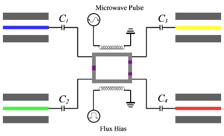
Figure 3: (color online). Diagram of a setup for four one-dimensional transmission line resonators coupled to a superconducting flux qutrit via capacitances $C_{1},C_{2},C_{3},$ and $C_{4}$, respectively.

We now provide a quantitative analysis on the experimental feasibility of the proposal. As an example, let us consider a setup of four one-dimensional transmission line resonators coupled by a superconducting flux qutrit (Fig. 3).

With the unwanted interaction being considered, the Hamiltonian (1) is modified as $H^{\prime}=H+\delta\!H_{1}+\delta\!H_{2}$ (with $N=2$), where $\delta\!H_{1}$ describes the unwanted inter-resonator crosstalk while $\delta\!H_{2}$ describes the unwanted $\left|e\right\rangle\leftrightarrow\left|f\right\rangle$ transition induced by the pulse. The expression of $\delta\!H_{1}$ is given by

$$\delta\!H_{1} = g_{a_{1}b_{1}}e^{i\Delta_{a_{1}b_{1}}t}a_{1}b_{1}^{+}+g_{a_{1}b_{2}}e^{i\Delta_{a_{1}b_{2}}t}a_{1}b_{2}^{+}$$ (16)

$$+g_{a_{2}b_{1}}e^{i\Delta_{a_{2}b_{1}}t}a_{2}b_{1}^{+}+g_{a_{2}b_{2}}e^{i\Delta_{a_{2}b_{2}}t}a_{2}b_{2}^{+}$$

$$+g_{a_{1}a_{2}}e^{i\Delta_{a_{1}a_{2}}t}a_{1}a_{2}^{+}+g_{b_{1}b_{2}}e^{i\Delta_{b_{1}b_{2}}t}b_{1}b_{2}^{+}+h.c.,$$

where $g_{a_{j}b_{k}}$ is the coupling strength between the two resonators $a_{j}$ and $b_{k}$ with frequency detuning $\Delta_{a_{j}b_{k}}=\omega_{b_{k}}-\omega_{a_{j}}$ ($j,k=1,2$); $g_{a_{1}a_{2}}$ is the coupling strength between the two resonators $a_{1}$ and $a_{2}$ with frequency detuning $\Delta_{a_{1}a_{2}}=\omega_{a_{2}}-\omega_{a_{1}};$ and $g_{b_{1}b_{2}}$ is the coupling strength between the two resonators $b_{1}$ and $b_{2}$ with frequency detuning $\Delta_{b_{1}b_{2}}=\omega_{b_{2}}-\omega_{b_{1}}$. $\delta\!H_{2}$ is given by

$$\delta\!H_{2}=\Omega_{fe}e^{i\Delta t}S_{fe}^{+}+\text{H.c.},$$ (17)

where $\Delta=\omega_{fe}-\omega_{eg},$ and $\Omega_{fe}$ is the pulse Rabi frequency associated with the $\left|e\right\rangle\leftrightarrow\left|f\right\rangle$ transition.

It should be mentioned that the $\left|g\right\rangle\leftrightarrow\left|f\right\rangle$ transition induced by the pulse is negligible because $\omega_{eg}\ll\omega_{fg}$ (Fig. 2). For simplicity, we also assume that the resonator-induced coherent transitions between any other irrelevant levels are negligibly small. This can be achieved by a prior design of the coupler with a sufficiently large anharmonicity of the level spacings (readily available for a superconducting flux device).

Taking into account the qutrit dephasing and energy relaxation as well as the resonator dissipation, the system dynamics, under the Markovian approximation, is determined by the master equation

$$\frac{d\rho}{dt} = -i\left[H^{\prime},\rho\right]+\sum\limits_{j=1}^{2}\kappa_{a_{j}}\mathcal{L}\left[a_{j}\right]+\sum\limits_{j=1}^{2}\kappa_{b_{j}}\mathcal{L}\left[b_{j}\right]$$ (18)

$$+\gamma_{fe}\mathcal{L}\left[\sigma_{fe}^{-}\right]+\gamma_{fg}\mathcal{L}\left[\sigma_{fg}^{-}\right]+\gamma_{eg}\mathcal{L}\left[\sigma_{eg}^{-}\right]$$

$$+\sum\limits_{l=e,f}\gamma_{\varphi,l}\left(\sigma_{ll}\rho\sigma_{ll}-\sigma_{ll}\rho/2-\rho\sigma_{ll}/2\right),$$

where $\mathcal{L}\left[\Lambda\right]=\Lambda\rho\Lambda^{+}-\Lambda^{+}\Lambda\rho/2-\rho\Lambda^{+}\Lambda/2$ (with $\Lambda=a_{j},b_{j},\sigma_{fe}^{-},\sigma_{fg}^{-},\sigma_{eg}^{-})$, $\sigma_{ee}=\left|e\right\rangle\left\langle e\right|,$ and $\sigma_{ff}=\left|f\right\rangle\left\langle f\right|$. In addition, $\kappa_{a_{j}}$ ($k_{b_{j}}$) is the decay rate of resonator $a_{j}$ ($b_{j}$); $\gamma_{eg}$ is the energy relaxation rate for the level $\left|e\right\rangle$ associated with the decay path $\left|e\right\rangle\rightarrow\left|g\right\rangle$; $\gamma_{fe}$ ($\gamma_{fg}$) is the relaxation rate for the level $\left|f\right\rangle$ related to the decay path $\left|f\right\rangle\rightarrow\left|e\right\rangle$ ($\left|f\right\rangle\rightarrow\left|g\right\rangle$); $\gamma_{\varphi,e}$ ($\gamma_{\varphi,f}$) is the dephasing rate of the level $\left|e\right\rangle$ ($\left|f\right\rangle$). For numerical calculations, here we use the QuTiP software [74,75]. QuTiP is an open-source software for simulating the dynamics of open quantum systems, which can transfer quantum objects to matrices and solve master equations numerically by using an ordinary differential equation solver.

Figure 4: (Color online) Fidelity versus the normalized detuning $c_{1}=\Delta_{1}/g_{1}$. Here and in Fig. 5, there is a relation, $c_{2}=\Delta_{2}/g_{2}=\sqrt{2}c_{1}$, for the $\Delta_{1}$ and $\Delta_{2}$ used in the numerical simulations.

The fidelity of the prepared two EPR states for the two pairs of photonic qubits is given by $\mathcal{F}=\sqrt{\left\langle\psi_{\mathrm{id}}\right|\widetilde{\rho}\left|\psi_{\mathrm{id}}\right\rangle}.$ Here, $\left|\psi_{\mathrm{id}}\right\rangle=\left|\text{EPR}\right\rangle_{a_{1}b_{1}}\otimes\left|\text{EPR}\right\rangle_{a_{2}b_{2}}$ is for the ideal case; while $\widetilde{\rho}$ is the reduced density operator of the two pairs of photonic qubits after tracing $\rho$ over the degrees of the coupler qutrit, when the operation is performed in a realistic system (with dissipation and dephasing considered).

In a real situation, it may be a challenge to obtain homogeneous coupling strengths. Thus, we consider $\mu_{1}=0.95g_{1}$ and $\mu_{2}=0.95g_{2}$ in our numerical simulation. Namely, there exists a difference of $5\%$ between the coupling strengths for each pair of resonators, which may be reasonable in experiments. Note that our numerical simulations are performed by choosing the operation time $t=\pi/\left(2\lambda\right)$ above, which is the operation time for an ideal homogeneous coupling.

For a three-level flux qutrit, the transition frequency between two neighboring levels can be varied from 5 GHz to 20 GHz. As an example, we consider $\omega_{eg}/2\pi=7.5$ GHz and $\omega_{fg}/2\pi=12.5$ GHz, for which we have $\Delta/2\pi=-2.5$ GHz. We set $\Delta_{1}/2\pi=0.75$ GHz and $\Delta_{2}/2\pi=1.5$ GHz, which yields $\Delta_{a_{1}a_{2}}/2\pi=\Delta_{b_{1}b_{2}}/2\pi=-0.75$ GHz, $\Delta_{a_{1}b_{1}}/2\pi=$ $\Delta_{a_{2}b_{2}}/2\pi=-7.5$ GHz, $\Delta_{a_{1}b_{2}}/2\pi=-8.25$ GHz, and $\Delta_{a_{2}b_{1}}/2\pi=-6.75$ GHz (Fig. 2). For simplicity, we choose $g_{a_{j}b_{k}}=g_{a_{1}a_{2}}=g_{b_{1}b_{2}}\equiv g_{cs}$ and $\Omega_{fe}=\Omega.$ Other parameters used in the numerical simulation are: (i) $\gamma_{\varphi,e}^{-1}=2.5$ $\mu$s, $\gamma_{\varphi,f}^{-1}=1.5$ $\mu$s, $\gamma_{eg}^{-1}=5$ $\mu$s, $\gamma_{fe}^{-1}=2.5$ $\mu$s, $\gamma_{fg}^{-1}=3.5$ $\mu$s (a conservative consideration, e.g., see Ref. [12]); and (ii) $\kappa_{a_{j}}^{-1}=\kappa_{b_{j}}^{-1}=10$ $\mu$s ($j=1,2$).

Figure 5: (color online). Fidelity versus $c_{1}$ and $\Omega$. The figure was plotted for $g_{cs}=0.4g_{m}$. Here, $c_{1}=\Delta_{1}/g_{1}$ is the normalized detuning and $\Omega$ is the Rabi frequency.

We now numerically calculate the fidelity for the two prepared EPR-pair states. For given values of $\Delta_{1},\Delta_{2},$ and $g_{1},$ the value of $g_{2}$ can be determined by Eq. (15). We define $c_{1}=\Delta_{1}/g_{1}$ and $c_{2}=\Delta_{2}/g_{2}.$ Based on Eq. (15), we have $c_{2}=\sqrt{\Delta_{2}/\Delta_{1}}c_{1}=\sqrt{2}c_{1}$ for the $\Delta_{1}$ and $\Delta_{2}$ chosen above. To see how the inter-resonator crosstalk affects the operation performance, in Fig. 4 we plot the fidelity versus $c_{1}$, by choosing $\Omega/2\pi=100$ MHz and considering $g_{cs}=0,0.2g_{m},0.4g_{m},0.6g_{m},0.8g_{m},g_{m}.$ Here and below, $g_{m}=\max\{g_{1},g_{2},\mu_{1},\mu_{2}\}.$ From Fig. 4, one can see that the effect of the inter-cavity crosstalk coupling is very small even when $g_{cs}=0.4g_{m}$, and a high fidelity $>97.86\%$ can be reached for $c_{1}=11$ (corresponding to $c_{2}=11\sqrt{2}$). In this case, the estimated operation time is $\sim 40$ ns. In the following analysis, we choose $g_{cs}=0.4g_{m}.$ Note that according to the discussion in [44], a smaller crosstalk $g_{cs}\leq 0.01g_{m}$ can be achieved with the typical capacitive cavity-qutrit coupling illustrated in Fig. 1.

We now consider the dependence of the operation performance on the value of the Rabi frequency $\Omega$ of the pulse. Figure 5 shows the fidelity versus $c_{1}$ and $\Omega.$ From Fig. 5, one can see that the operation performance strongly depends on the pulse Rabi frequency $\Omega$. On the other hand, Fig. 5 shows that for $c_{1}\in[7,17]$ ($c_{2}\in[7\sqrt{2},17\sqrt{2}]$), a high fidelity $\mathcal{F}\geq 92.4\%$ can be reached for a wide range of $\Omega$: $\Omega/2\pi\in[50,200]$ MHz. Note that a pulse Rabi frequency $\Omega/2\pi\sim 300$ MHz or higher was reported in experiments [76,77]. In Figure 5, the optimal point is $c_{1}=10.2$ ($c_{2}=10.2\sqrt{2}$) and $\Omega/2\pi=110$ MHz, for which the maximum fidelity of the joint state of the two prepared EPR pairs is $\mathcal{F}_{\max}=98.42\%$, corresponding to the fidelities $\mathcal{F}_{a_{1}b_{1}}=99.05\%$ and $\mathcal{F}_{a_{2}b_{2}}=99.07\%$ for the qubit pairs ($a_{1},b_{1}$) and ($a_{2},b_{2}$), respectively.

For $c_{1}\in[7,17]$ and $c_{2}\in[7\sqrt{2},17\sqrt{2}],$ we have $g_{1}/2\pi\in[107,44]$ MHz, $g_{2}/2\pi\in[151,62]$ MHz, $\mu_{1}/2\pi\in[102,42]$ MHz, and $\mu_{2}/2\pi\in[143,59]$ MHz. The coupling strengths of these values are readily achievable in experiments because a coupling strength $\sim 636$ MHz has been reported for a superconducting flux device coupled to a one-dimensional transmission line resonator [78]. For the transition frequencies of the qutrit and the detunings given above, we have $\omega_{a_{1}}/\left(2\pi\right)\sim 11.75$ GHz, $\omega_{a_{2}}/\left(2\pi\right)\sim 11$ GHz, $\omega_{b_{1}}/\left(2\pi\right)\sim 4.25$ GHz, and $\omega_{b_{2}}/\left(2\pi\right)\sim 3.5$ GHz. Thus, for the values of $\kappa_{a_{j}}^{-1}$ and $\kappa_{b_{j}}^{-1}$ used in the numerical simulation, the required quality factors for the four resonators are $Q_{a_{1}}\sim 7.4\times 10^{5},$ $Q_{a_{2}}\sim 6.8\times 10^{5},$ $Q_{b_{1}}\sim 2.7\times 10^{5},$ and $Q_{b_{2}}\sim 2.2\times 10^{5},$ available in experiments [21-23]. The analysis here demonstrates that the high-fidelity generation of two EPR pairs of photonic qubits distributed in the four resonators is feasible within present-day circuit QED techniques.

The prepared EPR pairs of photonic qubits can be read out by employing the conventional approach [79], i.e., mapping the states of the photonic qubits to superconducting qubits, whose states can be detected fast and accurately [80]. One can also use an alternative method introduced in [69] to measure the photonic qubits with a relatively fast speed and minimal action of decoherence.

V. CONCLUSION

We have presented an efficient method for simultaneously coupling multiple pairs of resonators by using a qutrit as a coupler. This proposal significantly reduces the effects of unwanted inter-resonator crosstalks which are inherent in a circuit consisting of two or more resonators. We showed that, under frequency matching conditions, the dynamics of the resonators is described by an effective Hamiltonian, which can be used for one-step generation of multiple EPR pairs of photonic qubits. Further, our numerical simulation demonstrated that the obtained EPR states can have high fidelities using present-day circuit QED technology. Finally, we note that this effective Hamiltonian has other applications. For instance, it can be directly applied to implement various quantum operations, such as the simultaneous transfer or exchange of multi-photon quantum states between spatially-separated resonators or cavities.

ACKNOWLEDGEMENTS

This work was partly supported by the RIKEN iTHES Project, the MURI Center for Dynamic Magneto-Optics via the AFOSR award number FA9550-14-1-0040, and a Grant-in-Aid for Scientific Research (A). It was also partially supported by the Major State Basic Research Development Program of China under Grant No. 2012CB921601, the National Natural Science Foundation of China under Grant Nos. [11074062, 11374083], the Zhejiang Natural Science Foundation under Grant No. LZ13A040002, the funds of Hangzhou Normal University under Grant Nos. [HSQK0081, PD13002004], and the funds of Hangzhou City for supporting the Hangzhou-City Quantum Information and Quantum Optics Innovation Research Team.

References

- (1) J. Clarke and F. K. Wilhelm, “Superconducting quantum bits”, Nature 453, 1031 (2008).
- (2) J. Q. You and F. Nori, “Atomic physics and quantum optics using superconducting circuits”, Nature 474, 589 (2011).
- (3) I. Buluta, S. Ashhab, and F. Nori, “Natural and artificial atoms for quantum computation”, Reports on Progress in Physics 74, 104401 (2011).
- (4) Z. L. Xiang, S. Ashhab, J. Q. You, and F. Nori, “Hybrid quantum circuits: Superconducting circuits interacting with other quantum systems”, Rev. Mod. Phys. 85, 623 (2013).
- (5) J. Bylander, S. Gustavsson, F. Yan, F. Yoshihara, K. Harrabi, G. Fitch, D. G. Cory, Y. Nakamura, J. S. Tsai, and W. D. Oliver, “ Noise spectroscopy through dynamical decoupling with a superconducting flux qubit”, Nature Phys. 7, 565 (2011).
- (6) H. Paik, D. I. Schuster, L. S. Bishop, G. Kirchmair, G. Catelani, A. P. Sears, B. R. Johnson, M. J. Reagor, L. Frunzio, L. I. Glazman, S. M. Girvin, M. H. Devoret, and R. J. Schoelkopf, “Observation of high coherence in Josephson Junction qubits measured in a three-dimensional circuit QED architecture”, Phys. Rev. Lett. 107, 240501 (2011).
- (7) J. B. Chang, M. R. Vissers, A. D. Córcoles, M. Sandberg, J. Gao, D. W. Abraham, J. M. Chow, J. M. Gambetta, M. B. Rothwell, G. A. Keefe, M. Steffen, and D. P. Pappas, “Improved superconducting qubit coherence using titanium nitride”, Appl. Phys. Lett. 103, 012602 (2013).
- (8) J. M. Chow, J. M. Gambetta, A. D. Córcoles, S. T. Merkel, J. A. Smolin, C. Rigetti, S. Poletto, G. A. Keefe, M. B. Rothwell, J. R. Rozen, M. B. Ketchen, and M. Steffen, “Universal quantum gate set approaching fault-tolerant thresholds with superconducting qubits”, Phys. Rev. Lett. 109, 060501 (2012).
- (9) R. Barends, J. Kelly, A. Megrant, D. Sank, E. Jeffrey, Y. Chen, Y. Yin, B. Chiaro, J. Y. Mutus, C. Neill, P. J. J. O’Malley, P. Roushan, J. Wenner, T. C. White, A. N. Cleland, and J. M. Martinis, “Coherent Josephson qubit suitable for scalable quantum integrated circuits”, Phys. Rev. Lett. 111, 080502 (2013).
- (10) J. M. Chow, J. M. Gambetta, E. Magesan, D. W. Abraham, A. W. Cross, B. R. Johnson, N. A. Masluk, C. A. Ryan, J. A. Smolin, S. J. Srinivasan, and M. Steffen, “Implementing a strand of a scalable fault-tolerant quantum computing fabric”, Nature Comm. 5, 4015 (2014).
- (11) Y. Chen, C. Neill, P. Roushan, N. Leung, M. Fang, R. Barends, J. Kelly, B. Campbell, Z. Chen, B. Chiaro, A. Dunsworth, E. Jeffrey, A. Megrant, J. Y. Mutus, P. J. J. O’Malley, C. M. Quintana, D. Sank, A. Vainsencher, J. Wenner, T. C. White, M. R. Geller, A. N. Cleland, and J. M. Martinis, “Qubit architecture with high coherence and fast tunable coupling”, Phys. Rev. Lett. 113, 220502 (2014).
- (12) M. Stern, G. Catelani, Y. Kubo, C. Grezes, A. Bienfait, D. Vion, D. Esteve, and P. Bertet, “Flux qubits with long coherence times for hybrid quantum circuits”, Phys. Rev. Lett. 113, 123601 (2014).
- (13) M. J. Peterer, S. J. Bader, X. Jin, F. Yan, A. Kamal, T. J. Gudmundsen, P. J. Leek, T. P. Orlando, W. D. Oliver, and S. Gustavsson,“Coherence and decay of higher energy levels of a superconducting transmon qubit”, Phys. Rev. Lett. 114, 010501 (2015).
- (14) F. Yan, S. Gustavsson, A. Kamal, J. Birenbaum, A. P. Sears, D. Hover, T. J. Gudmundsen, J. L. Yoder, T. P. Orlando, J. Clarke, A. J. Kerman, and W. D. Oliver, “The Flux qubit revisited”, arXiv:1508.06299.
- (15) C. P. Yang, S. I. Chu, and S. Han, “Possible realization of entanglement, logical gates, and quantum-information transfer with superconducting-quantum-interference-device qubits in cavity QED”, Phys. Rev. A 67, 042311 (2003).
- (16) J. Q. You and F. Nori, “Quantum information processing with superconducting qubits in a microwave field”, Phys. Rev. B 68, 064509 (2003).
- (17) A. Blais, R. S. Huang, A. Wallraff, S. M. Girvin, and R. J. Schoelkopf, “Cavity quantum electrodynamics for superconducting electrical circuits: An architecture for quantum computation”, Phys. Rev. A 69, 062320 (2004).
- (18) A. Wallraff, D. I. Schuster, A. Blais, L. Frunzio, R. S. Huang, J. Majer, S. Kumar, S. M. Girvin, and R. J. Schoelkopf, “Strong coupling of a single photon to a superconducting qubit using circuit quantum electrodynamics”, Nature 431, 162 (2004).
- (19) M. Hofheinz, H. Wang, M. Ansmann, R. C. Bialczak, E. Lucero, M. Neeley, A. D. O’Connell, D. Sank, J. Wenner, J. M. Martinis, and A. N. Cleland, “Synthesizing arbitrary quantum states in a superconducting resonator”, Nature 459, 546 (2009).
- (20) H. Wang, M. Hofheinz, J. Wenner, M. Ansmann, R. C. Bialczak, M. Lenander, E. Lucero, M. Neeley, A. D. O’Connell, D. Sank, M. Weides, A. N. Cleland, and J. M. Martinis, “Improving the coherence time of superconducting coplanar resonators”, Appl. Phys. Lett. 95, 233508 (2009).
- (21) W. Chen, D. A. Bennett, V. Patel, and J. E. Lukens, “Substrate and process dependent losses in superconducting thin film resonators Supercond”, Sci. Technol. 21, 075013 (2008).
- (22) P. J. Leek, M. Baur, J. M. Fink, R. Bianchetti, L. Steffen, S. Filipp, and A. Wallraff, “Cavity quantum electrodynamics with separate photon storage and qubit readout modes”, Phys. Rev. Lett. 104, 100504 (2010).
- (23) A. Megrant, C. Neill, R. Barends, B. Chiaro, Y. Chen, L. Feigl, J. Kelly, E. Lucero, M. Mariantoni, P. J. J. O’Malley, D. Sank, A. Vainsencher, J. Wenner, T. C. White, Y. Yin, J. Zhao, C. J. Palmstrøm, J. M. Martinis, and A. N. Cleland, “Planar superconducting resonators with internal quality factors above one million”, Appl. Phys. Lett. 100, 113510 (2012).
- (24) M. Reagor, W. Pfaff, C. Axline, R. W. Heeres, N. Ofek, K. Sliwa, E. Holland, C. Wang, J. Blumoff, K. Chou, M. J. Hatridge, L. Frunzio, M. H. Devoret, L. Jiang, R. J. Schoelkopf, “A quantum memory with near-millisecond coherence in circuit QED”, arXiv:1508.05882
- (25) I. Chiorescu, P. Bertet, K. Semba, Y. Nakamura, C. J. P. M. Harmans, and J. E. Mooij, “Coherent dynamics of a flux qubit coupled to a harmonic oscillator”, Nature 431, 159 (2004).
- (26) P. Forn-Díaz, J. Lisenfeld, D. Marcos, J. J. García-Ripoll, E. Solano, C. J. P. M. Harmans, and J. E. Mooij, “Observation of the Bloch-Siegert Shift in a Qubit-Oscillator System in the Ultrastrong Coupling Regime”, Phys. Rev. Lett. 105, 237001 (2010).
- (27) T. Niemczyk, F. Deppe, H. Huebl, E. P. Menzel, F. Hocke, M. J. Schwarz, J. J. Garcia-Ripoll, D. Zueco, T. Hümmer, E. Solano, A. Marx, and R. Gross, “Circuit quantum electrodynamics in the ultrastrong-coupling regime”, Nature Physics 6, 772 (2010)
- (28) R. Stassi, S. Savasta, L. Garziano, B. Spagnolo, and F. Nori, “Output field-quadrature measurements and qqueezing in ultrastrong cavity-QED”, arXiv:1509.09064
- (29) L. Garziano, R. Stassi, V. Macrì, A. F. Kockum, S. Savasta, and F. Nori, “Multiphoton quantum Rabi oscillations in ultrastrong cavity QED”, Phys. Rev. A 92, 063830 (2015).
- (30) F. Marquardt and C. Bruder, “Superposition of two mesoscopically distinct quantum states: Coupling a Cooper-pair box to a large superconducting island”, Phys. Rev. B 63, 054514 (2001).
- (31) Y. X. Liu, L. F. Wei, and F. Nori, “Generation of nonclassical photon states using a superconducting qubit in a microcavity”, Europhys. Lett. 67, 941 (2004).
- (32) Y. X. Liu, L. F. Wei, and F. Nori, “Preparation of macroscopic quantum superposition states of a cavity field via coupling to a superconducting charge qubit”, Phys. Rev. A 71, 063820 (2005).
- (33) M. Mariantoni, M. J. Storcz, F. K. Wilhelm, W. D. Oliver, A. Emmert, A. Marx, R. Gross, H. Christ, and E. Solano, “On-chip microwave Fock states and quantum homodyne measurements”, arXiv:cond-mat/0509737 (2005).
- (34) F. Marquardt, “Efficient on-chip source of microwave photon pairs in superconducting circuit QED”, Phys. Rev. B 76, 205416 (2007).
- (35) Y. J. Zhao, Y. L. Liu, Y. X. Liu, and F. Nori, “Generating nonclassical photon states via longitudinal couplings between superconducting qubits and microwave fields”, Phys. Rev. A 91, 053820 (2015).
- (36) M. Hofheinz, E. M. Weig, M. Ansmann, R. C. Bialczak, E. Lucero, M. Neeley, A. D. O’Connell, H. Wang, J. M. Martinis, and A. N. Cleland, “Generation of Fock states in a superconducting quantum circuit”, Nature 454, 310 (2008).
- (37) H. Wang, M. Hofheinz, M. Ansmann, R. C. Bialczak, E. Lucero, M. Neeley, A. D. O’Connell, D. Sank, J. Wenner, A. N. Cleland, and J. M. Martinis, “Measurement of the decay of Fock states in a superconducting quantum circuit”, Phys. Rev. Lett. 101, 240401 (2008).
- (38) F. W. Strauch, D. Onyango, K. Jacobs, R. W. Simmonds, Entangled State Synthesis for Superconducting Resonators, Phys. Rev. A 85, 022335 (2012).
- (39) R. Sharma and F. W. Strauch, Quantum State Synthesis of Superconducting Resonators, Phys. Rev. A 93, 012342 (2016).
- (40) M. Mariantoni, F. Deppe, A. Marx, R. Gross, F. K. Wilhelm, and E. Solano, “Two-resonator circuit quantum electrodynamics: A superconducting quantum switch”, Phys. Rev. B 78, 104508 (2008).
- (41) F. W. Strauch, K. Jacobs, and R. W. Simmonds, “Arbitrary control of entanglement between two superconducting resonators”, Phys. Rev. Lett. 105, 050501 (2010).
- (42) S. T. Merkel and F. K. Wilhelm, “Generation and detection of NOON states in superconducting circuits”, New J. Phys. 12, 093036 (2010).
- (43) Q. P. Su, C. P. Yang, and S. B. Zheng, “Fast universal quantum gates on microwave photons with all-resonance operations in circuit QED”, Sci. Rep. 4, 3898 (2014); S. J. Xiong, Z. Sun, J. M. Liu, T. Liu, and C. P. Yang, “Efficient scheme for generation of photonic NOON states in circuit QED”, Opt. Lett. 40, 2221 (2015).
- (44) C. P. Yang, Q. P. Su, and S. Han, “Generation of Greenberger-Horne-Zeilinger entangled states of photons in multiple cavities via a superconducting qutrit or an atom through resonant interaction”, Phys. Rev. A 86, 022329 (2012).
- (45) C. P. Yang, Q. P. Su, S. B. Zheng, and S. Han, “Generating entanglement between microwave photons and qubits in multiple cavities coupled by a superconducting qutrit”, Phys. Rev. A 87, 022320 (2013); M. Hua, M. J. Tao, and F. G. Deng, “One-step implementation of entanglement generation on microwave photons in distant 1D superconducting resonators”, arXiv:1508.00061
- (46) Y. J. Zhao, C. Q. Wang, X. Zhu, and Y. X. Liu, “Engineering entangled microwave photon states via multiphoton transitions between two cavities and a superconducting qubit”, arXiv:1506.06363
- (47) M. Hua, M. J. Tao, and F. G. Deng, “Universal quantum gates on microwave photons assisted by circuit quantum electrodynamics”, Phys. Rev. A 90, 012328 (2014).
- (48) M. Hua, M. J. Tao, and F. G. Deng, “Fast universal quantum gates on microwave photons with all-resonance operations in circuit QED”, Scientific Reports 5, 9274 (2015).
- (49) H. Wang, M. Mariantoni, R. C. Bialczak, M. Lenander, E. Lucero, M. Neeley, A. D. O’Connell, D. Sank, M. Weides, J. Wenner, T. Yamamoto, Y. Yin, J. Zhao, J. M. Martinis, and A. N. Cleland, “Deterministic entanglement of photons in two superconducting microwave resonators”, Phys. Rev. Lett. 106, 060401 (2011).
- (50) M. Mariantoni, H. Wang, R. C. Bialczak, M. Lenander, E. Lucero, M. Neeley, A. D. O’Connell, D. Sank, M. Weides, J. Wenner, T. Yamamoto, Y. Yin, J. Zhao, J. M. Martinis, and A. N. Cleland, “Photon shell game in three-resonator circuit quantum electrodynamics”, Nat. Phys. 7, 287 (2011).
- (51) A. Einstein, B. Podolsky, and N. Rosen, “Can quantum-mechanical description of Finite precision nullifies the K-S theorem David A. Meyer physical reality be considered complete”, Phys. Rev. 47, 777 (1935).
- (52) A. Bramon and M. Nowakowski, “Bell Inequalities for Entangled Pairs of Neutral Kaons”, Phys. Rev. Lett. 83, 1 (1999).
- (53) E. Solano, R. L. de Matos Filho, and N. Zagury, “Deterministic Bell states and measurement of the motional state of two trapped ions”, Phys. Rev. A 59, R2539 (1999).
- (54) K. Lake, S. Weidt, J. Randall, E. D. Standing, S. C. Webster, and W. K. Hensinger, Generation of spin-motion entanglement in a trapped ion using long-wavelength radiation, Phys. Rev. A 91, 012319 (2015).
- (55) J. I. Cirac and P. Zoller, “Preparation of macroscopic superpositions in many-atom systems”, Phys. Rev. A 50, R2799 (1994).
- (56) S. B. Zheng and G. C. Guo, “Efficient scheme for two-atom entanglement and quantum information processing in cavity QED”, Phys. Rev. Lett. 85, 2392 (2000).
- (57) W. Li, C. Li , and H. Song, “The preparation of Bell state using ground state of -type Rb atoms in two optical cavities”, Optical and Quantum Electronics 46, 1561 (2014).
- (58) S. L. Su, X. Q. Shao, Q. Guo, L. Y. Cheng, H. F. Wang, and S. Zhang, “Preparation of entanglement between atoms in spatially separated cavities via fiber loss”, Eur. Phys. J. D 69, 123 (2015).
- (59) Q. Y. He, M. D. Reid, T. G. Vaughan, C. Gross, M. Oberthaler, and P. D. Drummond, “Einstein-Podolsky-Rosen Entanglement Strategies in Two-Well Bose-Einstein Condensates”, Phys. Rev. Lett. 106, 120405 (2011).
- (60) Q. Y. He, P. D. Drummond, M. K. Olsen, and M. D. Reid, “Einstein-Podolsky-Rosen entanglement and steering in two-well BEC ground states”, Phys. Rev. A 86, 023626 (2012).
- (61) B. Opanchuk, Q. Y. He, M. D. Reid, P. D. Drummond, “Dynamical preparation of EPR entanglement in two-well Bose-Einstein condensates”, Phys. Rev. A 86, 023625 (2012).
- (62) R. Schmidt, J. T. Stockburger, and J. Ankerhold, “Almost local generation of Einstein-Podolsky-Rosen entanglement in nonequilibrium open systems”, Phys. Rev. A 88, 052321 (2013).
- (63) Roman Schnabel, “Einstein-Podolsky-Rosen–entangled motion of two massive objects”, Phys. Rev. A 92, 012126 (2015).
- (64) L. F. Wei, Y. X. Liu, M. J. Storcz, and F. Nori, “Macroscopic Einstein-Podolsky-Rosen pairs in superconducting circuits”, Phys. Rev. A 73, 052307 (2006).
- (65) F. Reiter, L. Tornberg, G. Johansson, and A. S. Sørensen, Steady-state entanglement of two superconducting qubits engineered by dissipation”, Phys. Rev. A 88, 032317 (2013).
- (66) C. P. Yang, Q. P. Su, and F. Nori, “Entanglement generation and quantum information transfer between spatially-separated qubits in different cavities”, New J. Phys. 15, 115003 (2013).
- (67) D. F. V. James and J. Jerke, “Effective Hamiltonian theory and its applications in quantum information”, Can. J. Phys. 85, 625 (2007).
- (68) A. Sørensen and K. Mølmer, “Quantum computation with ions in thermal motion”, Phys. Rev. Lett. 82, 1971 (1999).
- (69) M. J. Storcz, M. Mariantoni, H. Christ, A. Emmert, A. Marx, W. D. Oliver, R. Gross, F. K. Wilhelm, E. Solano, “Orthogonally-Driven Superconducting Qubit in Circuit QED”, arXiv:cond-mat/0612226
- (70) E. Solano, G. S. Agarwal, and H. Walther, “Strong-Driving-Assisted Multipartite Entanglement in Cavity QED”, Phys. Rev. Lett. 90, 027903 (2003).
- (71) F. Motzoi, J. M. Gambetta, P. Rebentrost, and F. K. Wilhelm, “Simple Pulses for Elimination of Leakage in Weakly Nonlinear Qubits”, Phys. Rew. Lett. 103, 110501 (2009).
- (72) Z. Chen et al., “Measuring and Suppressing Quantum State Leakage in a Superconducting Qubit”, Phys. Rev. Lett. 116, 020501 (2016).
- (73) X. Y. Jin, A. Kamal, A. P. Sears, T. Gudmundsen, D. Hover, J. Miloshi, R. Slattery, F. Yan, J. Yoder, T. P. Orlando, S. Gustavsson, and W. D. Oliver, “Thermal and Residual Excited-State Population in a 3D Transmon Qubit”, Phys. Rev. Lett. 114, 240501 (2015).
- (74) J. R. Johansson, P. D. Nation, and F. Nori, “QuTiP: An open-source Python framework for the dynamics of open quantum systems”, Comp. Phys. Comm. 183, 1760 (2012).
- (75) J. R. Johansson, P. D. Nation, and F. Nori, “QuTiP 2: A Python framework for the dynamics of open quantum systems”, Comp. Phys. Comm. 184, 1234 (2013).
- (76) M. Baur, S. Filipp, R. Bianchetti, J. M. Fink, M. Göppl, L. Steffen, P. J. Leek, A. Blais, and A. Wallraff, “Measurement of Autler-Townes and Mollow transitions in a strongly driven superconducting qubit”, Phys. Rev. Lett. 102, 243602 (2009).
- (77) F. Yoshihara, Y. Nakamura, F. Yan, S. Gustavsson, J. Bylander, W. D. Oliver, and J. S. Tsai, “Flux qubit noise spectroscopy using Rabi oscillations under strong driving conditions”, Phys. Rev. B 89, 020503(R) (2014).
- (78) T. Niemczyk, F. Deppe, H. Huebl, E. P. Menzel, F. Hocke, M. J. Schwarz, J. J. Garcia-Ripoll, D. Zueco, T. Hümmer, E. Solano, A. Marx, and R. Gross, “Circuit quantum electrodynamics in the ultrastrong-coupling regime”, Nature Phys. 6, 772 (2010).
- (79) W. H. Zurek, “Decoherence, einselection, and the quantum origins of the classical”, Rev. Mod. Phys. 75, 715 (2003).
- (80) M. D. Reed, L. DiCarlo, B. R. Johnson, L. Sun, D. I. Schuster, L. Frunzio, and R. J. Schoelkopf, “High-Fidelity Readout in Circuit Quantum Electrodynamics Using the Jaynes-Cummings Nonlinearity”, Phys. Rev. Lett. 105, 173601 (2010).