The stretched exponential behavior and its underlying dynamics. The phenomenological approach

Abstract

We show that the anomalous diffusion equations with a fractional spacial derivative in the Caputo or Riesz sense are strictly related to the special convolution properties of the Lévy stable distributions which stem from the evolution properties of stretched or compressed exponential function. The formal solutions of these fractional differential equations are found by using the evolution operator method where the evolution is conceived as integral transform whose kernel is the Green function. Exact and explicit examples of the solutions are reported and studied for various fractional order of derivatives and for different initial conditions.

MSC 2010: Primary 35R11; Secondary 26A33, 60G18, 60G52, 49M20

Key Words and Phrases: fractional calculus, stretched or compressed exponential function, fractional ordinary and partial differential equations, Green functions

I Introduction

In recent experiments of relaxation processes in a variety of complex materials and systems, such as supercooled liquids, spin glasses, amorphous solids, molecular systems, glass soft matter, porous and noncrystaline silicon, etc. WGotze92 ; JCPhillips96 ; CAAngell00 ; LCipelletti05 ; LPavesi96 ; IMihalcescu96 , the relaxation properties have been successfully fitted by stretched exponentials RKohlrausch54 ; GWilliams70 ; RSAnderssen04

$$f_{\alpha}(\mbox{$\frac{t}{\tau_{0}}$})=e^{-\big{(}\mbox{$\frac{t}{\tau_{0}}$}\big{)}^{\alpha}},\quad\text{for}\quad t>0\quad\text{and}\quad 0<\alpha<1,$$

called also the Kohlrausch-Williams-Watts functions (the KWW functions). Moreover, it has been shown, e.g. in KWeron96 , that the KWW function is related to the Cole-Cole relaxation processes which appear in the systems of disordered or anomalous structures. The importance of the KWW function for the survival propability in relation to relaxation function has been also noted and dissed in KWeron96 . The decay according to the KWW pattern is by no means restricted to common relaxation phenomena. For example, it appears in biological context, e.g. in protein folding JSabelko99 and in $\alpha$-Helix formation in photo-switchable peptides JBredenbeck05 ; JAIhalainen07 , etc. The stretched exponential behavior is also used to describe the local variations of transport speed YZhang07 ; BDybiec08 . Exponential decay faster than the Debye law ($\alpha>1$) is also observed. This case is called the compressed exponential, which in the theory of slow magnetization is named the Kolmogorov-Avrami-Fatuzzo relaxation HXi08 ; AAdanlete11 ; NZurauskiene14 .

The function $f_{\alpha}(t/\tau_{0})$ is related to Lévy stable distributions HPollard46 ; HBergstrom52 : for $0<\alpha<1$ these are one-sided and for $1<\alpha\leq 2$ these are two-sided cases. As it is known there exists an intimate relation between the Lévy stable distributions and the anomalous diffusion; for $0<\alpha<1$ it is the sub-diffusion and for $1<\alpha\leq 2$ it is the super-diffusion. We are going to approach this connection in a novel way. The physical formulation is based on the Fokker-Planck equation with the spatial fractional derivative, usually of Riemann-Liouville, Caputo or Riesz types. The case of $\alpha=2$ is matched with the standard diffusion equation. For $\alpha\equiv N=3,4,5\ldots$ the compressed exponential functions correspond to the partial differential equation with the space derivative of order $N$ KGorska13 ; EOrsinger12 . The sub- and super-diffusion equations are usually derived via the probability approach like the continuous-time random walks JKlafter80 , the master equation DBedeaux71 , the generalized master equation VMKenkre73 , and related methods ACompte96 ; MMagdziarz06 ; BDybiec10 . The intense activity in this field has apparently been initiated by Saichev and Zaslavsky in AISaichev97 . The relevant references can be traced back from two recent papers ECapelasdeOliverira14 ; RGarra14 . A very complete and lucid exposition of theoretical aspects of diffusion phenomena can be found in MMeerschaert12 . Nevertheless, the anomalous diffusion equations should stem from the natural evolution property which is satisfied by $f_{\alpha}(t/\tau_{0})$: namely a suitably defined product of two stretched (compressed) exponential functions should give another stretched (compressed) exponential function. From the mathematical point of view, the use of the complex analysis technique underlying this condition will allow us to obtain the fractional Fokker-Planck equations. This alternative approach to a derivation of the anomalous equations and the operational method of solving them are the main objectives of this work. We believe that this will open new possibilities of looking at the stretched and compressed exponentials which have in the natural way built-in the anomalous behavior.

The paper is organized as follows. In Sec. II we recall and comment on two relations: the first is between the stretched exponential and the one-sided Lévy stable distribution, and the second one is between the compressed exponential and two-sided Lévy stable distribution. We use the well-known unique relation between the one- and two-variables Lévy stable distributions whose evolution property will be studied in the paper. In Sec. II we derive two types of integral evolution equations related to two various behaviors of $f_{\alpha}(t/\tau_{0})$. The differential version of these equations will be found in Sec. III. In connection with the used Lévy stable distribution they will contain the fractional derivative in the Caputo or Riesz sense. The solution of these differential equations in terms of the Green function are given in Sec. IV. Sec. V is devoted to finding the solution of these equations with the help of operational methods based on the integral transforms whose kernels are given by the appropriate Lévy stable distributions. Sec. VI contains the explicit examples of solutions of the equations. We conclude the paper in Sec. VII.

II Lévy stable distributions

In a discrete setting and from a phenomenological point of view the KWW functions for $0<\alpha<1$ can be treated as a sum of weight function of exponential decays ($f_{\alpha}(t/\tau_{0})$ for $\alpha=1$) GDattoli14 , namely

$$f_{\alpha}(\mbox{$\frac{t}{\tau_{0}}$})=\sum_{j}e^{-\frac{t}{\tau_{0}}u_{j}}g_{\alpha}(u_{j})\Delta u_{j},$$ (1)

where $g_{\alpha}(u_{j})$ is a probability density, i.e. $g_{\alpha}(u_{j})>0$ and $\sum_{j}g_{\alpha}(u_{j})\Delta u_{j}~{}=~{}1$, which describes the structure of the sample where relaxation process is governed by the stretched exponential function. In the limit of large number of elements in the sum and for the infinitesimally small changes $\Delta u_{i}$, Eq. (1) goes over to the Laplace transform GDattoli14 ; KWeron91

$$f_{\alpha}(\mbox{$\frac{t}{\tau_{0}}$})=\mathcal{L}\left[g_{\alpha}(u);\mbox{$\frac{t}{\tau_{0}}$}\right] =\int_{0}^{\infty}e^{-\frac{t}{\tau_{0}}u}g_{\alpha}(u)du$$ (2)

$$=\int_{0}^{\infty}e^{-x}g_{\alpha}((\mbox{$\frac{t}{\tau_{0}}$})^{\alpha},x)dx.$$ (3)

In Eq. (2) the variable of integration is changed to $u~{}=~{}\tau_{0}x/t$ and it gives the relation VMZolotarev83 ; KGorska12 ; KAPenson16 :

$$\mbox{$\frac{\tau_{0}}{t}$}g_{\alpha}(\mbox{$\frac{\tau_{0}}{t}$}x)\equiv g_{\alpha}((\mbox{$\frac{t}{\tau_{0}}$})^{\alpha},x).$$ (4)

Systematic treatment of relations of type Eq. (4) can be rephrased in terms of subordination laws, consequences of the properties of Mellin transform BDybiec10 ; KAPenson16 ; FMainardi03 . Eq. (4) represents the one-to-one correspondence between the one- and two- variables Lévy stable distributions. It leads to the evolution equation with the fractional derivative which will be studied below. In this sense Eq. (4) is crucial for our considerations.

In order to limit the proliferation of notation we shall employ the same symbol to both sides of Eq. (4), and later on, to Eq. (10). Their meaning will be clear from the context and should not lead to confusion.

The probability density $g_{\alpha}((\mbox{$\frac{t}{\tau_{0}}$})^{\alpha},x)$, via the inverse Laplace transform of Eq. (2) and Eq. (4), is uniquely given by one-sided Lévy stable distributions HPollard46 :

$$\begin{split}g_{\alpha}((\mbox{$\frac{t}{\tau_{0}}$})^{\alpha},x)&=\mathcal{L}^{-1}\{\exp[-\big{(}\mbox{$\frac{t}{\tau_{0}}$}\xi\big{)}^{\alpha}];x\}\\ &=\frac{1}{2\pi i}\int_{L}e^{x\xi}e^{-\big{(}\mbox{$\frac{t}{\tau_{0}}$}\xi\big{)}^{\alpha}}d\xi,\end{split}$$ (5)

$x>0$, and $g_{\alpha}((\mbox{$\frac{t}{\tau_{0}}$})^{\alpha},x)=0$ for $x\leq 0$. We remark that the Laplace transform $f_{L}(p)$ of the function $f(u)$ is defined as follows INSneddon74 :

$$f_{L}(p)=\mathcal{L}[f(u);p]=\int_{0}^{\infty}e^{-up}f(u)du,$$

for $p\in\mathbb{C}$, whereas the inverse Laplace transform is given by

$$f(u)=\mathcal{L}^{-1}[f_{L}(p);u]=\frac{1}{2\pi i}\int_{L}e^{up}f_{L}(p)dp,$$

where inside the integration contour $L$ the function $f_{L}(p)$ is analytic. Eq. (5) goes to the Dirac $\delta$ function, namely $\delta(u)$, in the limit of $t\to 0$, see (ISGradsteyn07, , Eq. (17.13.94) on p. 1115). The function $g_{\alpha}((\mbox{$\frac{t}{\tau_{0}}$})^{\alpha},x)$ has the essential singularity at $x=0$ (JMikusinski59, , Eq. (4)) and the “heavy” long tail as $x\to\infty$ (JMikusinski59, , Eq. (5)). Taking in Eq. (5) the integral contour $L$ defined in HPollard46 and using Eq. (4), we get

$$g_{\alpha}((\mbox{$\frac{t}{\tau_{0}}$})^{\alpha},x)={\rm Im}\left\{\int_{0}^{\infty}e^{-x\xi}e^{-(\frac{t}{\tau_{0}}\xi)^{\alpha}e^{-i\pi\alpha}}\frac{d\xi}{\pi}\right\},$$ (6)

which for rational $0<\alpha=l/k<1$ is equal to

$$\begin{split}g_{\frac{l}{k}}((\mbox{$\frac{t}{\tau_{0}}$})^{\frac{l}{k}},x)&=\sum_{j=1}^{k-1}\frac{(-1)^{j}x^{-1-j\frac{l}{k}}}{j!\,\Gamma(-\frac{l}{k}j)}\left(\!\frac{t}{\tau_{0}}\!\right)^{j\frac{l}{k}}\\ &\times{{}_{l+1}F_{k}}\left({1,\Delta(l,1+j\frac{l}{k})\atop\Delta(k,1+j)}\Big{|}z\right),\end{split}$$ (7)

with $z=(-1)^{k-l}(tl)^{l}/[k^{k}(\tau_{0}x)^{l}]$, see KAPenson10 . The generalized hypergeometric function is denoted as ${{}_{n}F_{m}}\left({(\alpha_{n})\atop(\beta_{m})}\Big{|}x\right)$, where $(\alpha_{n})$ is the “upper” list of parameters and $(\beta_{m})$ is the “lower” list APPrudnikov_v3 . The symbol $\Delta(n,a)$ is equal to a list of $n$ elements $\frac{a}{n},\frac{a+1}{n},\ldots,\frac{a+n-1}{n}$. The basic example of $g_{l/k}((\mbox{$\frac{t}{\tau_{0}}$})^{l/k},x)$ is the so-called Lévy-Smirnov distribution $g_{1/2}((\mbox{$\frac{t}{\tau_{0}}$})^{1/2},x)=\sqrt{t/\tau_{0}}\exp[-(t/\tau_{0})/(4x)]/(2\sqrt{\pi}x^{3/2})$. The other explicit and exact examples of $g_{\alpha}((\mbox{$\frac{t}{\tau_{0}}$})^{l/k},x)$ can be obtained by using Eq. (4) and further examples are quoted in KAPenson10 .

The compressed exponential behavior can be written as $f_{\alpha}(t/\tau_{0})=\mbox{$\frac{1}{2}$}f_{\alpha}(|t/\tau_{0}|)$, which for $1<\alpha<2$ is related via the Fourier transform INSneddon74 to $\tilde{g}_{\alpha}(u)$, the two-sided Lévy distribution,

$$f_{\alpha}(\mbox{$\frac{t}{\tau_{0}}$})=\mbox{$\frac{1}{2}$}f_{\alpha}(|\mbox{$\frac{t}{\tau_{0}}$}|) =\mathcal{F}\left[\mbox{$\frac{1}{2}$}\tilde{g}_{\alpha}(u);\mbox{$\frac{t}{\tau_{0}}$}\right]$$

$$=\int_{-\infty}^{\infty}e^{i\mbox{$\frac{t}{\tau_{0}}$}u}\,\mbox{$\frac{1}{2}$}\tilde{g}_{\alpha}(u)du$$ (8)

$$=\int_{-\infty}^{\infty}e^{ix}\,\mbox{$\frac{1}{2}$}\tilde{g}_{\alpha}((\mbox{$\frac{t}{\tau_{0}}$})^{\alpha},x)dx,$$ (9)

where, similarly to Eqs. (2) and (3), we use the new variable of integration $x$. Let us recall that the Fourier transform $g_{F}(\omega)$ of the function $g(x)$ is given by

$$g_{F}(\omega)=\mathcal{F}[g(x);\omega]=\int_{-\infty}^{\infty}e^{-i\omega x}g(x)dx,$$

where

$$g(x)=\mathcal{F}^{-1}[g_{F}(\omega);x]=\frac{1}{2\pi}\int_{-\infty}^{\infty}e^{i\omega x}g_{F}(\omega),$$

which is the inverse Fourier transform. In analogy to Eq. (4) we get the unique scaling relation

$$\mbox{$\frac{\tau_{0}}{t}$}\tilde{g}_{\alpha}(\mbox{$\frac{\tau_{0}}{t}$}x)\equiv\tilde{g}_{\alpha}((\mbox{$\frac{t}{\tau_{0}}$})^{\alpha},x),$$ (10)

whose evolution property will be studied in this work. The inversion of the Fourier transform given in Eq. (II) and the use of property (10) leads to

$$\begin{split}\tilde{g}_{\alpha}((\mbox{$\frac{t}{\tau_{0}}$})^{\alpha},x)&=\mathcal{F}^{-1}\{\exp[-\big{(}\!\mbox{$\frac{t}{\tau_{0}}$}\!\big{)}^{\alpha}|\xi|^{\alpha}];x\}\\ &=\int_{-\infty}^{\infty}e^{-ix\xi}e^{-\big{(}\!\mbox{$\frac{t}{\tau_{0}}$}\!\big{)}^{\alpha}|\xi|^{\alpha}}\frac{d\xi}{2\pi}\end{split}$$ (11)

for $x\in\mathbb{R}$ and $t>0$, which is the symmetric two-sided Lévy stable distribution, see Eq. (8) for $\beta=0$ of HBergstrom52 applied for (10). Observe that Eq. (11) defines also the symmetric Lévy stable distribution for $0<\alpha<1$ HBergstrom52 ; KGorska11 . In the limit of vanishing $t$ the two-sided Lévy stable distribution goes to the Dirac $\delta$ function, i.e. $\tilde{g}_{\alpha}((\mbox{$\frac{t}{\tau_{0}}$})^{\alpha},x)\to\delta(x)$ for $t\to 0$. Eq. (11) expressed as the finite sum of the generalized hypergeometric function is given in (KGorska11, , Eqs. (4) and (5) for $l=2p$, $k=2q$, and $r=p$), namely

$$\tilde{g}_{\frac{p}{q}}((\mbox{$\frac{t}{\tau_{0}}$})^{\frac{p}{q}},x) =\sum_{j=1}^{M-1}\frac{(-1)^{1+j}}{\pi\,j!}\,\Gamma\left(1+\frac{m}{M}j\right)\frac{(t/\tau_{0})^{\mp\frac{2p}{M}j}}{x^{1\mp\frac{2p}{M}j}}$$

$$\times{{}_{m+1}F_{M}}\left({1,\Delta(m,1+\frac{m}{M}j)\atop\Delta(M,1+j)}\Big{|}\tilde{z}\right),$$ (12)

where $\tilde{z}=(-1)^{p-M}[t/(\tau_{0}x)]^{\mp 2p}\,m^{m}/M^{M}$, $m=\min(2p,2q)$, $M=\max(2p,2q)$. The lower sign in the powers of $t/\tau_{0}$ and $x$ is for $p<q$, whereas the upper sign is for $p>q$. For $\alpha=2$ we get the Gauss (normal) distribution, $\tilde{g}_{2}((t/\tau_{0})^{2};x)=\tau_{0}\exp[-(x\tau_{0})^{2}/(2t)^{2}]/(4\sqrt{\pi}t)$. For more examples see KGorska11 .

From the very natural evolution assumption written for the stretched (compressed) exponential function for $t_{0}\leq t_{1}\leq t_{2}$, it appears that an appropriately defined composition of two stretched (compressed) exponentials should give another stretched (compressed) exponential. It means that the appropriate convolution of the stable distributions of two variables gives another stable distribution of two variables: (i) for the one-sided Lévy stable distribution of two variables we have

$$g_{\alpha}((\mbox{$\frac{t_{2}-t_{0}}{\tau_{0}}$})^{\alpha},x)\!=\!\int_{0}^{x}\!\!\!g_{\alpha}((\mbox{$\frac{t_{2}-t_{1}}{\tau_{0}}$})^{\alpha},y)g_{\alpha}((\mbox{$\frac{t_{1}-t_{0}}{\tau_{0}}$})^{\alpha},x-y)dy,$$ (13)

whereas (ii) for the two-sided Lévy stable distribution of two variables we get

$$\tilde{g}_{\alpha}((\mbox{$\frac{t_{2}-t_{0}}{\tau_{0}}$})^{\alpha},x)\!=\!\int_{-\infty}^{\infty}\!\!\!\tilde{g}_{\alpha}((\mbox{$\frac{t_{2}-t_{1}}{\tau_{0}}$})^{\alpha},y)\tilde{g}_{\alpha}((\mbox{$\frac{t_{1}-t_{0}}{\tau_{0}}$})^{\alpha},x-y)dy.$$ (14)

The proofs of Eqs. (13) and (14) are given in Appendix A. Eqs. (13) and (14) are the new types of Laplace and Fourier convolutions, respectively, where both of the arguments of functions, i.e. $t$ and $x$, vary. We point out that Eqs. (13) and (14) differ from the standard Laplace and Fourier convolutions of the one variable Lévy stable distributions which lead to the stable laws VMZolotarev83 ; WFeller71 . For the stretched exponential the stable law has the form

$$e^{-(b_{1}p)^{\alpha}}e^{-(b_{2}p)^{\alpha}}=e^{-(bp)^{\alpha}}\quad\text{for}\quad b_{1}^{\alpha}+b_{2}^{\alpha}=b^{\alpha}.$$

Eqs. (13) and (14) are the integral forms of the evolution equations whose differential forms will be found in the next section.

The properties inherent in Eqs. (13) and (14) naturally illustrate the transitivity of evolution expressed in two-variable version of $g_{\alpha}$’s and $\tilde{g}_{\alpha}$’s. Apparently, these extensions were not employed in the current context before.

III Fractional differential equation related to Lévy stable distributions

III.1 The differential form of Eq. (13)

We start by rephrasing Eq. (13) for $(t_{2}-t_{1})/\tau_{0}=T$ and infinitesimally small $(t_{1}-t_{0})/\tau_{0}=\Delta T$. The r.h.s of Eq. (13) can be estimated by taking the asymptotics of $g_{\alpha}((\Delta T)^{\alpha},x-y)$ for $\Delta T\ll 1$. Using Eq. (6), where instead of $\exp[-(\Delta T\xi)^{\alpha}e^{-i\pi\alpha}]$ we take its first two terms of asymptotic expansion, i.e. $1-(\Delta T\,\xi)^{\alpha}e^{-i\pi\alpha}$, we obtain

$$g_{\alpha}((\Delta T)^{\alpha},x-y)\simeq{\rm Im}\left\{\int_{0}^{\infty}e^{-(x-y)\xi}\frac{d\xi}{\pi}\right\}$$ (1)

$$\quad-{\rm Im}\left\{(\Delta T)^{\alpha}e^{-i\pi\alpha}\int_{0}^{\infty}e^{-(x-y)\xi}\xi^{\alpha}\frac{d\xi}{\pi}\right\}$$ (2)

$$\quad={\rm Im}\left\{\frac{1}{\pi(x-y)}-(\Delta T)^{\alpha}e^{-i\pi\alpha}\frac{\Gamma(1+\alpha)}{\pi(x-y)^{1+\alpha}}\right\}.$$ (3)

In Eqs. (1) and (2) we employed (APPrudnikov_v1, , Eq. (2.3.3.1) on p. 322). Substitution of Eq. (3) into Eq. (13) written for $(t_{2}-t_{1})/\tau_{0}=T$ and $(t_{1}-t_{0})/\tau_{0}=\Delta T$ gives

$$\text{RHS of Eq. }(\ref{eq13})={\rm Im}\left\{\int_{0}^{x}\frac{g_{\alpha}(T^{\alpha},y)}{x-y}\frac{dy}{\pi}\right\}$$ (4)

$$\qquad-{\rm Im}\left\{\frac{(\Delta T)^{\alpha}}{e^{i\pi\alpha}}\Gamma(1+\alpha)\int_{0}^{x}\frac{g_{\alpha}(T^{\alpha},y)}{(x-y)^{1+\alpha}}\frac{dy}{\pi}\right\}.$$ (5)

The integral in Eq. (4) can be calculated by inserting Eq. (6) into it, and then changing the order of integration. That leads to

$${\rm Im}\left\{\int_{0}^{x}\frac{g_{\alpha}(T^{\alpha},y)}{x-y}\frac{dy}{\pi}\right\}={\rm Im}\left\{\int_{0}^{\infty}e^{-(T\xi)^{\alpha}\exp(-i\alpha\pi)}\right\}$$

$$\qquad\times\left.{\rm Im}\left[\int_{0}^{x}\frac{e^{-y\xi}}{x-y}dy\right]\frac{d\xi}{\pi^{2}}\right\}$$ (6)

$$\qquad={\rm Im}\left\{\int_{0}^{\infty}e^{-x\xi}e^{-(T\xi)^{\alpha}\exp(-i\alpha\pi)}\frac{d\xi}{\pi}\right\}$$ (7)

$$\qquad=g_{\alpha}(T^{\alpha},x).$$

The second integral in Eq. (III.1) is calculated in Appendix B and it is equal to $\pi e^{-x\xi}$, see Eq. (5). In Eq. (7) we employ the definition given in Eq. (6).

Next, we calculate the integral in Eq. (5) as follows: we apply $(x-y)^{-\alpha-1}=\frac{1}{\alpha}\frac{d}{dy}(x-y)^{-\alpha}$, integrate Eq. (5) by parts and use the definition of the one-sided Lévy stable distribution in Eq. (6). Thus,

$${\rm Im}\left\{\frac{\Gamma(1+\alpha)}{e^{i\pi\alpha}}\int_{0}^{x}\frac{g_{\alpha}(T^{\alpha},y)}{(x-y)^{1+\alpha}}\frac{dy}{\pi}\right\}$$

$$\qquad\qquad=\Gamma(\alpha)\,{\rm Im}\left[\lim_{y\to x}\frac{g_{\alpha}(T^{\alpha},y)}{(y-x)^{\alpha}}\right]$$ (8)

$$\qquad\qquad-{\rm Im}\left[\frac{\Gamma(\alpha)}{e^{i\pi\alpha}}\int_{0}^{x}\frac{g^{\prime}_{\alpha}(T^{\alpha},y)}{(x-y)^{\alpha}}\frac{dy}{\pi}\right],$$ (9)

where $g^{\prime}_{\alpha}(T^{\alpha},y)=\frac{d}{dy}g_{\alpha}(T^{\alpha},y)$. From the theory of residues FWByron92 the limit in Eq. (8) is equal to

$$\lim_{y\to x}\frac{g_{\alpha}(T^{\alpha},y)}{(y-x)^{\alpha}}=\frac{1}{2\pi i}\oint_{S_{\delta}}\frac{g_{\alpha}(T^{\alpha},z)}{(z-x)^{\alpha}}dz.$$ (10)

The contour $S_{\delta}$ is a circle around $x$ with the radius $\delta$ ($\delta\ll 1$) in a counterclockwise manner. Inserting Eq. (6) into Eq. (10) and changing the order of integration we have

$${\rm Im}\left[\lim_{y\to x}\frac{g_{\alpha}(T^{\alpha},y)}{(y-x)^{\alpha}}\right] ={\rm Im}\left\{\int_{0}^{\infty}e^{-(T\xi)^{\alpha}\exp(-i\pi\alpha)}\right.$$

$$\times\left.{\rm Im}\left[\frac{1}{2\pi i}\oint_{S_{\delta}}\frac{e^{-z\xi}}{(z-x)^{\alpha}}dz\right]\frac{d\xi}{\pi}\right\}.$$

Setting $z-x=\delta e^{i\varphi}$ and then taking the limit of small $\delta$ we obtain that the integral over closed contour $S_{\delta}$ has only the real value which is equal to $e^{-x\xi}$. That leads to vanishing of the integral and consequently to vanishing Eq. (8). Consequently, Eq. (9) is equal to

$${\rm Im}\left[\frac{\Gamma(\alpha)}{e^{i\pi\alpha}}\int_{0}^{x}\frac{g^{\prime}_{\alpha}(T^{\alpha}y)}{(x-y)^{\alpha}}\frac{dy}{\pi}\right]=\int_{0}^{x}\frac{g^{\prime}_{\alpha}(T^{\alpha},y)}{(x-y)^{\alpha}}\frac{dy}{\Gamma(1-\alpha)},$$ (11)

which follows from (ISGradsteyn07, , Eq. (8.334.3)) and the fact that the integral in Eq. (11) is real. That can be shown by calculating the derivative of $g_{\alpha}(T^{\alpha},y)$ given in Eq. (6), inserting it in Eq. (9), changing the order of integration, and using (ISGradsteyn07, , Eq. (3.381.1) on p. 346).

Expressing the l.h.s. of Eq. (13) written for $(t_{2}~{}-~{}t_{1})/\tau_{0}=T$ and infinitesimally small $(t_{1}-t_{0})/\tau_{0}=\Delta T$ into the Taylor series up to the second term we get

$$g_{\alpha}((T+\Delta T)^{\alpha},x)\simeq g_{\alpha}(T^{\alpha},x)+\partial_{T^{\alpha}}g_{\alpha}(T^{\alpha},x)$$

$$\qquad\times[(T+\Delta T)^{\alpha}-T^{\alpha}]$$ (12)

$$\qquad\simeq g_{\alpha}(T^{\alpha},x)+(\Delta T)^{\alpha}\partial_{T^{\alpha}}g_{\alpha}(T^{\alpha},x),$$ (13)

where in Eq. (III.1) we employed the asymptotics of the square bracket, namely $[(T+\Delta T)^{\alpha}-T^{\alpha}]\simeq(\Delta T)^{\alpha}$.

Collecting together all the contributions we obtain that the right hand side of Eq. (13) for $(t_{2}-t_{1})/\tau_{0}=T$ and $(t_{1}-t_{0})/\tau_{0}=\Delta T$, where $\Delta T\ll 1$, has the form specified below:

$$\partial_{T^{\alpha}}g_{\alpha}(T^{\alpha},x)=-\,{{}^{C}\!\partial_{x}^{\alpha}}g_{\alpha}(T^{\alpha},x),\quad 0<\alpha<1.$$ (14)

In Eq. (14) ${{}^{C}\!\partial_{x}^{\alpha}}g_{\alpha}(T^{\alpha},x)$ denotes the so-called fractional derivative in the Caputo sense IPodlubny99 ; SGSamko93 ; Mainardi1

$${{}^{C}\!\partial_{x}^{\alpha}}f(x)=\frac{1}{\Gamma(1-\alpha)}\int_{0}^{x}\frac{f^{\prime}(y)dy}{(x-y)^{\alpha}},$$

where $0<\alpha<1$ and $f^{\prime}(y)=\frac{d}{dy}f(y)$.

III.2 The differential form of Eq. (14)

Let us now find the differential form of Eq. (14) for $(t_{2}-t_{1})/\tau_{0}=T$ and $(t_{1}-t_{0})/\tau_{0}=\Delta T$ such that $\Delta T\ll 1$. Similarly to the approach presented in the previous subsection we will estimate the r.h.s. of Eq. (14) for infinitesimally small values of $\Delta T$. Employing Eq. (11) adjusted for $\tilde{g}_{\alpha}((\Delta T)^{\alpha},x-y)$ and taking the asymptotic expansion of $\exp[-(\Delta T)^{\alpha}|\xi|^{\alpha}]$ up to the second term, we obtain

$$\tilde{g}_{\alpha}((\Delta T)^{\alpha},x-y)\simeq\int_{-\infty}^{\infty}e^{-i(x-y)\xi}[1-(\Delta T)^{\alpha}|\xi|^{\alpha}]\frac{d\xi}{2\pi}$$

$$\qquad=\delta(x-y)-\frac{(\Delta T)^{\alpha}}{2}\frac{|x-y|^{-1-\alpha}}{\cos(\mbox{$\frac{\alpha\pi}{2}$})\Gamma(-\alpha)}.$$ (15)

In Eq. (III.2) we have used formulas (1.1) on p. 102 and (1.11) on p. 103 of YABrychkov77 . Inserting Eq. (III.2) into the r.h.s. of Eq. (14) gives

$$\begin{split}\text{RHS of Eq. }(\ref{eq14})&=\tilde{g}_{\alpha}(T^{\alpha},x)-\frac{(\Delta T)^{\alpha}}{2\Gamma(-\alpha)\cos(\mbox{$\frac{\pi\alpha}{2}$})}\\ &\times\int_{-\infty}^{\infty}\frac{\tilde{g}_{\alpha}(T^{\alpha},y)}{|x-y|^{1+\alpha}}dy.\end{split}$$ (16)

The integral in Eq. (16) is related to the fractional derivative in the Riesz sense RGorenflo98 ; SGSamko93 :

$${{}^{R}\partial_{|x|}^{\alpha}}f(x)=-\frac{1}{2\Gamma(-\alpha)\cos(\mbox{$\frac{\alpha\pi}{2}$})}\int_{-\infty}^{\infty}\frac{f(y)\,dy}{|x-y|^{1+\alpha}}$$ (17)

for $0<\alpha<1$.

The first two terms of the Taylor series of the l.h.s. of Eq. (14) read

$$\tilde{g}_{\alpha}((T+\Delta T)^{\alpha},x)\simeq\tilde{g}_{\alpha}(T^{\alpha},x)+(\Delta T)^{\alpha}\,\partial_{T^{\alpha}}\tilde{g}_{\alpha}(T^{\alpha},x),$$ (18)

which is in analogy to Eq. (13). Substituting Eqs. (18), (16) and (17) into Eq. (14) with $(t_{2}-t_{1})/\tau_{0}=T$ and infinitesimally small $(t_{1}-t_{0})/\tau_{0}=\Delta T$ we obtain

$$\partial_{T^{\alpha}}\tilde{g}_{\alpha}(T^{\alpha},x)={{}^{R}\partial_{|x|}^{\alpha}}\tilde{g}_{\alpha}(T^{\alpha},x)$$ (19)

for $1<\alpha\leq 2$, see also Mainardi1 ; Mainardi .

IV The Green function method

We recall the fundamental facts about the propagator and the Green function, compare FWByron92 . We consider the differential equation in the form

$$\partial_{y}h(y,x)=\hat{O}h(y,x),$$ (1)

where an operator $\hat{O}=\hat{O}(x,\frac{d}{dx})$ is independent on $y$. Its formal solution for $y>y^{\prime}$ can be given by

$$h(y,x)=\int K(y,x;y^{\prime},x^{\prime})h(y^{\prime},x^{\prime})dx^{\prime}.$$

The function $K(y,x;y^{\prime},x^{\prime})$ is a propagator related to Eq. (1) which is an response of the system on the given initial (or boundary) conditions which are the Dirac $\delta$ functions. The propagator $K$ has the following properties: (i) $K(y,x;y,x^{\prime})=\delta(x-x^{\prime})$; (ii) $(\partial_{y}-\hat{O})K(y,x;y^{\prime},x^{\prime})=0$; and (iii) for $y_{0}\leq y_{1}\leq y_{2}$ the propagator satisfies $K(y_{2},x_{2};y_{0},x_{0})=\int K(y_{2},x_{2};y_{1},x_{1})K(y_{1},x_{1};y_{0},x_{0})dx_{1}$, which is the Laplace convolution for the one-sided Lévy stable distribution and the Fourier convolution for the two-sided Lévy distribution.

$K(y,x;y^{\prime},x^{\prime})$ can be used to define the Green function $G(y,x;y^{\prime},x^{\prime})$, which fulfills

$$(\partial_{y}-\hat{O})G(y,x;t^{\prime},x^{\prime})=\delta(x-x^{\prime})\delta(y-y^{\prime}).$$ (2)

The relation between the propagator and the Green function is given by

$$G(y,x;y^{\prime},x^{\prime})=\Theta(y-y^{\prime})K(y,x;y^{\prime},x^{\prime})+AK(y,x;y^{\prime},x^{\prime}),$$ (3)

where $\Theta(y-y^{\prime})$ is the Heaviside step function and $A$ is a constant.

IV.1 The Green function of Eq. (14)

In this subsection we will find the Green function relevant to Eq. (14) denoted by $G(T^{\alpha},x;\tilde{T}^{\alpha},\tilde{x})$. For that purpose we solve Eq. (2) with $\hat{O}=-{{}^{C}\!\partial_{x}^{\alpha}}$ and $y=(t/\tau_{0})^{\alpha}\equiv T^{\alpha}$ by taking twice the Laplace transform of this equation and applying (ISGradsteyn07, , Eq. (17.13.95) on p. 1115). The twofold use of Laplace transform, one in $T^{\alpha}$ ($T>0$) and another one in $x$ ($x>0$) gives

$$\mathcal{L}\left[\mathcal{L}\left[(\partial_{T^{\alpha}}+{{}^{C}\!\partial_{x}^{\alpha}})G(T^{\alpha},x;\tilde{T}^{\alpha},\tilde{x});\tau\right];\kappa\right]\!=\!e^{-\tau\tilde{T}^{\alpha}}e^{-\kappa\tilde{x}},$$

where $T>\tilde{T}$. The Laplace transform of the first derivative with respect to $T^{\alpha}$ is proportional to $\tau$, i.e. $\mathcal{L}[\partial_{T^{\alpha}}G(T^{\alpha},x;\tilde{T}^{\alpha},\tilde{x});\tau]=\tau G_{L_{\tau}}(\tau,x;\tilde{T}^{\alpha},\tilde{x})$. Similarly the Laplace transform of the fractional derivative in the Caputo sense of $G(T^{\alpha},x;\tilde{T}^{\alpha},\tilde{x})$ is given by $\kappa^{\alpha}G_{L_{\kappa}L_{\tau}}(\tau,\kappa;\tilde{T}^{\alpha},\tilde{x})-\kappa^{\alpha-1}G(T^{\alpha},\tilde{x};\tilde{T}^{\alpha},\tilde{x})$, see (IPodlubny99, , Eq. (2.140) on p. 80 for $0<\alpha<1$) or (VKiryakova13, , Eq. (6) for $0<\alpha<1$). The symbols $L_{\tau}$ and $L_{\kappa}$ denote the Laplace transforms with respect to time $T^{\alpha}$ and space $x$ such that $G_{L_{\kappa}L_{\tau}}(\tau,\kappa;t^{\prime},x^{\prime})=\mathcal{L}[\mathcal{L}[G(T^{\alpha},x;\tilde{T}^{\alpha},\tilde{x});\tau];\kappa]$. Assuming that $G(T^{\alpha},\tilde{x};\tilde{T}^{\alpha},\tilde{x})=0$, we get

$$G_{L_{\kappa}L_{\tau}}(\tau^{\alpha},\kappa;\tilde{T}^{\alpha},\tilde{x})=\frac{e^{-\tau\tilde{T}^{\alpha}}e^{-\kappa\tilde{x}}}{\tau+\kappa^{\alpha}},$$ (4)

Thus, the Green function $G(T^{\alpha},x;\tilde{T}^{\alpha},\tilde{x})$ can be obtained by taking twice the inverse Laplace transform of Eq. (4):

$$G(T^{\alpha},x;\tilde{T}^{\alpha},\tilde{x})=\mathcal{L}^{-1}[\mathcal{L}^{-1}[G_{L_{\kappa}L_{\tau}}(\tau,\kappa;\tilde{T}^{\alpha},\tilde{x});T^{\alpha}];x]$$

$$\qquad=\mathcal{L}^{-1}\left[\Theta(T^{\alpha}-\tilde{T}^{\alpha})e^{-\kappa\tilde{x}}e^{-(T^{\alpha}-\tilde{T}^{\alpha})\kappa^{\alpha}};x\right]$$

$$\qquad=\Theta(x-\tilde{x})\Theta(T^{\alpha}-\tilde{T}^{\alpha})g_{\alpha}(T^{\alpha}-\tilde{T}^{\alpha},x-\tilde{x}).$$ (5)

In Eq. (IV.1) we have applied (INSneddon74, , Eq. (3-3-11) on p. 146 of vol. 2) and the definition of the one-sided Lévy stable distribution. Comparing Eqs. (IV.1) and (3) we have $A=0$ and

$$K(T^{\alpha},x;\tilde{T}^{\alpha},\tilde{x})=\Theta(x-\tilde{x})g_{\alpha}(T^{\alpha}-\tilde{T}^{\alpha},x-\tilde{x})$$

with $g_{\alpha}(T^{\alpha}-\tilde{T}^{\alpha};x-\tilde{x})$ given in Eq. (5). From the properties of the one-sided Lévy stable distribution it can be seen that the propagator $K$ satisfies properties (i), (ii) and (iii) which are listed at the beginning of this Section. The property (ii) can be easily shown to hold by demonstrating that the Laplace transform $\mathcal{L}[(\partial_{T^{\alpha}}+{{}^{C}\!\partial^{\alpha}_{x}})\Theta(x-\tilde{x})g_{\alpha}(T^{\alpha}-\tilde{T}^{\alpha};x-\tilde{x});\kappa]$ vanishes. It comes from (INSneddon74, , Eq. (3-3-11) on p. 146) and (IPodlubny99, , Eq. (2.140) on p. 80). The property (iii) is proven in Appendix A.

IV.2 The Green function of Eq. (19)

The Green function $\tilde{G}(T^{\alpha},x;\tilde{T}^{\alpha},\tilde{x})$ for $T>\tilde{T}$ which is the solution of Eq. (19), i.e. Eq. (2) with $\hat{O}=-\,{{}^{R}\partial_{|x|}^{\alpha}}$ and $y=(t/\tau)^{\alpha}\equiv T^{\alpha}$, can be obtained by taking the Laplace transform in $T^{\alpha}$ for $T>0$ and Fourier transform in $x$ for $x\in\mathbb{R}$:

$$\mathcal{F}\!\left[\mathcal{L}\!\left[(\partial_{T^{\alpha}}-\,{{}^{R}\partial_{|x|}^{\alpha}})\tilde{G}(T^{\alpha}\!,x;\tilde{T}^{\alpha}\!,\tilde{x});\tau\right]\!\!;\kappa\right]=e^{-\tau\tilde{T}^{\alpha}}.$$ (6)

The Fourier transform of the fractional derivative in the Riesz sense is equal to $-|\kappa|^{\alpha}\tilde{G}_{F_{\kappa}}(T^{\alpha},\kappa;\tilde{T}^{\alpha},\tilde{x})$, see (RGorenflo98, , Eq. (1.17)) and SGSamko93 . Thus, Eq. (6) reads

$$\tilde{G}_{F_{\kappa}L_{\tau}}(\tau,\kappa;\tilde{T}^{\alpha},\tilde{x})=\frac{e^{-\tau\tilde{T}^{\alpha}}}{\tau+|\kappa|^{\alpha}},$$

where $\tilde{G}_{F_{\kappa}L_{\tau}}(\tau,\kappa;\tilde{T}^{\alpha},\tilde{x})=\mathcal{F}[\mathcal{L}[\tilde{G}(T^{\alpha},x;\tilde{T}^{\alpha},\tilde{x});\tau];\kappa]$. After calculating the inverse Laplace transform and then the inverse Fourier transform of $\tilde{G}_{F_{\kappa}L_{\tau}}(\tau,\kappa;t^{\prime},x^{\prime})$, we get

$$\tilde{G}(T^{\alpha},x;\tilde{T}^{\alpha},\tilde{x}) =\mathcal{F}^{-1}[\mathcal{L}^{-1}[\tilde{G}_{F_{\kappa}L_{\tau}}(\tau,\kappa;\tilde{T}^{\alpha},\tilde{x});T^{\alpha}];x]$$

$$=\mathcal{F}^{-1}[\Theta(T^{\alpha}-\tilde{T}^{\alpha})e^{-T^{\alpha}|\kappa|^{\alpha}};x]$$

$$=\Theta(T^{\alpha}-\tilde{T}^{\alpha})\tilde{g}_{\alpha}(T^{\alpha}-\tilde{T}^{\alpha},x-\tilde{x}).$$ (7)

The two-sided Lévy stable distribution $\tilde{g}_{\alpha}(T^{\alpha}-\tilde{T}^{\alpha},x-\tilde{x})$ is defined in Eq. (11). Comparison of Eq. (IV.2) with Eq. (3) indicates that $A=0$ and propagator $\tilde{K}$ is given by

$$\tilde{K}(T^{\alpha},x;\tilde{T}^{\alpha},\tilde{x})=\tilde{g}_{\alpha}(T^{\alpha}-\tilde{T}^{\alpha},x-\tilde{x}).$$ (8)

We stress that the properties of $\tilde{g}_{\alpha}(T^{\alpha},x)$ imply that the requirements (i)-(iii) are satisfied for $\tilde{K}$ defined in Eq. (8). For example, the property (ii) follows from (INSneddon74, , Eq. (2-3-8) on p. 39 of vol. 1) and (RGorenflo98, , Eq. (1.17)).

V The evolution operator method

V.1 The case of Eq. (14)

From the mathematical point of view, Eq. (14) with the initial condition $h(x)$ is the Cauchy-like problem. Its formal solution for $x>0$ and $0<\alpha<1$ can be expressed via evolution operator $\hat{U}_{\alpha}(T)$ in the following way

$$g_{\alpha}(T^{\alpha},x)=\hat{U}_{\alpha}(T)h(x)=\exp(-T^{\alpha}\,{{}^{C}\!\partial_{x}^{\alpha}})h(x)$$ (1)

$$\qquad=\int_{0}^{\infty}g_{\alpha}(T^{\alpha},\xi)h(x-\xi)d\xi,$$ (2)

The second equality in Eq. (1) has a symbolic meaning which suggests naively employing a series representation of $\hat{U}_{\alpha}(T)$. This series representation does not constitute an effective tool because the series obtained usually converges for fixed $T$ only and for special values of initial conditions. The use of integral representation, see Eq. (2), for an established domain of $\hat{U}_{\alpha}(T)$ avoids the problem of convergence and opens the new way of finding and obtaining the mathematically correct solutions.

The integral kernel $g_{\alpha}(T^{\alpha};x)$, given in Eqs. (6) and (7), is a special solution of Eq. (2) for the initial condition $h(x)=\delta(x)$. It is also the propagator $K(T^{\alpha},x;\tilde{T}^{\alpha},\tilde{x})$ for $\tilde{T}=0$ and $\tilde{x}=0$. Eq. (2) for $h(x)=g_{\alpha}(0;x)$ reconstructs the convolution property Eq. (13) for $(t_{2}-t_{1})/\tau_{0}=T$ and $(t_{1}-t_{0})/\tau_{0}=0$. It can be also shown that for different times $t_{0}$, $t_{1}$ and $t_{2}$ such that $t_{0}\leq t_{1}\leq t_{2}$, the evolution operator satisfies

$$\hat{U}_{\alpha}(\mbox{$\frac{t_{2}-t_{0}}{\tau_{0}}$})=\hat{U}_{\alpha}(\mbox{$\frac{t_{2}-t_{1}}{\tau_{0}}$})\hat{U}_{\alpha}(\mbox{$\frac{t_{1}-t_{0}}{\tau_{0}}$}).$$ (3)

which follows from Eq. (13).

Let us now establish the conditions under which Eq. (2) solves Eq. (14). For that purpose we calculate the Laplace transform of the both sides of Eq. (14). Thus, we get

$$\mathcal{L}[\partial_{T^{\alpha}}g_{\alpha}(T^{\alpha},x);\kappa]=\partial_{T^{\alpha}}e^{-(T\kappa)^{\alpha}}=-\kappa^{\alpha}e^{-(T\kappa)^{\alpha}},$$ (4)

where we applied Eq. (2). The r.h.s of Eq. (14), where we employed Eq. (2) and (IPodlubny99, , Eq. (2.140) on p. 80 for $0<\alpha<1$), reads

$$\mathcal{L}[{{}^{C}\!\partial^{\alpha}_{x}}g_{\alpha}(T^{\alpha},x);\kappa] =\mathcal{L}\left[\int_{0}^{\infty}g_{\alpha}(T^{\alpha},\xi){{}^{C}\!\partial^{\alpha}_{x}}h(x-\xi)d\xi;\kappa\right]$$

$$=\int_{0}^{\infty}g_{\alpha}(T^{\alpha},\xi)\mathcal{L}[{{}^{C}\!\partial^{\alpha}_{x}}h(x-\xi);\kappa]d\xi$$

$$=\int_{0}^{\infty}g_{\alpha}(T^{\alpha},\xi)\kappa^{\alpha}\mathcal{L}[h(x-\xi);\kappa]$$

$$-\int_{0}^{\infty}g_{\alpha}(T^{\alpha},\xi)d\xi\,\kappa^{\alpha-1}h(0)$$

$$=\kappa^{\alpha}e^{-(T\kappa)^{\alpha}}-\kappa^{\alpha-1}h(0).$$ (5)

If we assume that the Laplace transform of $h(x)$ exists, i.e. $\mathcal{L}[h(x);\kappa]=H(\kappa)$, $h(0)=0$, and we change the sign like in Eq. (14), then Eq. (5) is equal to Eq. (4). That implies that $g_{\alpha}(t;x)$ given in Eq. (2) is the solution of Eq. (14).

The inverse Laplace transform of $h(x-\xi)$, which is equal to $e^{-\xi\kappa}\mathcal{L}^{-1}[H(\kappa);x]$, implies that the formal solution (2) obtained by using the evolution operator method has also the form:

$$g_{\alpha}(T^{\alpha},x)=\mathcal{L}^{-1}[e^{-(T\kappa)^{\alpha}}H(\kappa);x],$$ (6)

which allows one to rewrite $g_{\alpha}(T^{\alpha},x)$ in terms of the inverse Mellin transform INSneddon74

$$g_{\alpha}(T^{\alpha},x)=\mathcal{M}^{-1}\left[\int_{0}^{\infty}\frac{\kappa^{-s}e^{-(T\kappa)^{\alpha}}}{\Gamma(1-s)}H(\kappa)d\kappa;x\right],$$

where we applied (JSLew75, , Eq. (2.1)).

V.2 The case of Eq. (19)

The formal solution obtained via the evolution operator method of Eq. (19) with the initial condition $\tilde{h}(x)$, can be presented as

$$\tilde{g}_{\alpha}(T^{\alpha},x) =\hat{V}_{\alpha}(T)\tilde{h}(x)=e^{T^{\alpha}{{}^{R}\!\partial^{\alpha}_{|x|}}}\tilde{h}(x)$$

$$=\int_{-\infty}^{\infty}\tilde{g}_{\alpha}(T^{\alpha},\xi)\tilde{h}(x-\xi)d\xi.$$ (7)

Similarly, like in the case of the operator $\hat{U}_{\alpha}(T)$, the integral representation (7) frees us from using the series representation of $\hat{V}_{\alpha}(T)$ which, even for well-defined initial conditions, can lead to divergent solutions.

The integral kernel $\tilde{g}_{\alpha}(T^{\alpha},\xi)$ is the two-sided Lévy stable distribution, see Eqs. (11) and (12), which is a special solution of Eq. (19) with the initial condition $\tilde{h}(x)=\delta(x)$. It is the propagator $\tilde{K}(T^{\alpha},x;\tilde{T}^{\alpha},\tilde{x})$, see Eq. (8), for $\tilde{T}=0$ and $\tilde{x}=0$. Eq. (7) reproduces the convolution property Eq. (14) for $\tilde{h}(x)=\tilde{g}_{\alpha}(0,x)$. In analogy to Eq. (3), it can be shown that for $t_{0}\leq t_{1}\leq t_{2}$ the condition

$$\hat{V}_{\alpha}(\mbox{$\frac{t_{2}-t_{0}}{\tau_{0}}$})=\hat{V}_{\alpha}(\mbox{$\frac{t_{2}-t_{1}}{\tau_{0}}$})\hat{V}_{\alpha}(\mbox{$\frac{t_{1}-t_{0}}{\tau_{0}}$})$$

is satisfied which stems form Eq. (14).

Taking the Fourier transform of both sides of Eq. (19) with $\tilde{g}_{\alpha}(T^{\alpha},x)$ defined in Eq. (7), we check that it is the correct solution of this differential equation. The Fourier transform of Eq. (19) gives:

$$\mathcal{F}[\partial_{T^{\alpha}}\tilde{g}_{\alpha}(T^{\alpha},x);\kappa]=\partial_{t}e^{-T^{\alpha}|\kappa|^{\alpha}}=-|\kappa|^{\alpha}e^{-T^{\alpha}|\kappa|^{\alpha}},$$ (8)

where we employed Eq. (11). The Fourier transform of the r.h.s. of Eq. (19) reads

$$\mathcal{F}[{{}^{R}\!\partial_{|x|}^{\alpha}}\tilde{g}_{\alpha}(T^{\alpha},x);\kappa]=\mathcal{F}\left[\int_{-\infty}^{\infty}\tilde{g}_{\alpha}(T^{\alpha},x){{}^{R}\!\partial_{|x|}^{\alpha}}\tilde{h}(x-\xi)d\xi;\kappa\right]$$

$$\qquad=\int_{-\infty}^{\infty}\tilde{g}_{\alpha}(T^{\alpha},x)\mathcal{F}[{{}^{R}\!\partial_{|x|}^{\alpha}}\tilde{h}(x-\xi);\kappa]d\xi$$ (9)

$$\qquad=-|\kappa|^{\alpha}\mathcal{F}\left[\int_{-\infty}^{\infty}\tilde{g}_{\alpha}(T^{\alpha},x)\tilde{h}(x-\xi)d\xi;\kappa\right]$$

$$\qquad=-|\kappa|^{\alpha}\mathcal{F}\left[\tilde{g}_{\alpha}(T^{\alpha},x);\kappa\right].$$

Using Eq. (II) we obtain Eq. (8) which completes the proof. In Eq. (9) we employed (RGorenflo98, , Eq. (1.17)) and assume that the Fourier transform of $\tilde{h}(x)$ exists and is equal to $\mathcal{F}[\tilde{h}(x);\kappa]=\tilde{H}(\kappa)$.

VI Examples

(A) We start with finding the formal solution of Eqs. (14) and (19) for the initial conditions given by the one- and two-sided Lévy stable distributions, $h(x)=g_{\beta}(0,x)$ and $\tilde{h}(x)=\tilde{g}_{\beta}(0,x)$, respectively. If the values of $\beta$ are the same as in the integral kernel of Eqs. (2) and (7), i.e. $\beta=\alpha$, then we get the convolution properties Eqs. (13) and (14) for $(t_{2}-t_{1})/\tau_{0}=T$ and $(t_{1}-t_{0})/\tau_{0}=0$. For $\beta\neq\alpha$ the formal solutions given in Eqs. (2) and (7) are presented in KGorska15 .

(B) Eq. (2) for the integral kernel $g_{1/2}(\sqrt{T},\xi)$ given by the Lévy-Smirnov distribution and the initial condition $h(x)=(\pi x)^{-1/2}[1-\exp(-\mbox{$\frac{1}{4x}$})]$ will be solved by using Eq. (6). The Laplace transform of $h(x)$ is obtained by using (APPrudnikov_v1, , Eq. (2.3.3.1) on p. 322 and Eq. (2.3.16.2) on p. 344) and is equal to $H(\kappa)=\kappa^{-1/2}(1-e^{-\sqrt{\kappa}})$. Inserting it into Eq. (6), employing for the Mellin transform $\mathcal{M}[f(x);s]=f_{M}(s)$ the formulas (APPrudnikov_v3, , Eqs. (8.4.1.4), (8.4.1.7) and (8.4.1.5) on p. 531), i.e. $\mathcal{M}^{-1}[a^{s}f_{M}(s);x]=\mathcal{M}^{-1}[f_{M}(s);\mbox{$\frac{x}{a}$}]$, $\mathcal{M}^{-1}[f_{M}(-s);x]=\mathcal{M}^{-1}[f_{M}(s);x^{-1}]$ and $\mathcal{M}^{-1}[f_{M}(s+a);x]=x^{a}\mathcal{M}^{-1}[f_{M}(s);x]$, we get

$$g^{(B)}_{1/2}(\sqrt{T},x) =\frac{1}{\sqrt{\pi x}}\mathcal{M}^{-1}\left[\Gamma(s);\frac{T}{4x}\right]$$

$$-\frac{1}{\sqrt{\pi x}}\mathcal{M}^{-1}\left[\Gamma(s);\frac{(1+\sqrt{T})^{2}}{4x}\right].$$

From (FOberhettinger74, , Eq.(5.1) on p. 191) $g^{(B)}_{1/2}(\sqrt{T},x)$ reads

$$g^{(B)}_{1/2}(\sqrt{T},x)=\frac{1}{\sqrt{\pi x}}\left[e^{-\mbox{$\frac{T}{4x}$}}-e^{-\mbox{$\frac{(\sqrt{T}+1)^{2}}{4x}$}}\right],$$

see also Fig. 1, for different values of $T$.

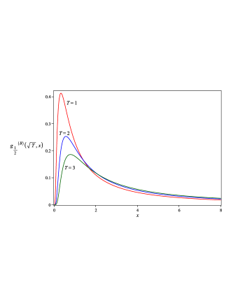
Figure 1: The plot of $g^{(B)}_{1/2}(\sqrt{T},x)$ for $T=1$ (red curve), $T=2$ (blue curve), and $T=3$ (green curve).

(C) The formal solution given in Eq. (7) with the integral kernel being the Gauss distribution and the initial condition

$$h(x)=\frac{1}{b-a}\left\{\begin{array}[]{c c c}0,&\text{for}&-\infty<x<a\\ 1,&\text{for}&a\leq x\leq b\\ 0,&\text{for}&b<x<\infty\end{array}\right.$$

can be calculated as follows

$$g^{(C)}_{2}(T^{2},x) =\int_{-\infty}^{\infty}\frac{1}{2T\sqrt{\pi}}e^{-\xi^{2}/(4T^{2})}h(x-\xi)d\xi$$

$$=\frac{1}{2T\sqrt{\pi}(b-a)}\int_{x-b}^{x-a}e^{-\xi^{2}/(4T^{2})}d\xi$$ (1)

$$=\frac{1}{2(b-a)}\left[{\rm erf}\left(\frac{b-x}{2T}\right)-{\rm erf}\left(\frac{a-x}{2T}\right)\right],$$

and is plotted in Fig. 2 for several values of $T$. In Eq. (VI) we have employed (ISGradsteyn07, , Eq. (2.33.2) on p. 108).

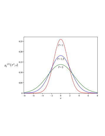
Figure 2: The plot of $g^{(C)}_{2}(T^{2},x)$ for $a=-1$, $b=1$, and $T=1$ (red curve), $T=1.5$ (blue curve), and $T=2$ (green curve).

All the initial conditions chosen above are normalizable. Consequently, the evolution solutions of (A), (B) and (C) conserve the normalizability. We observed also that non-normalizable initial conditions, not considered here, lead to evolution solutions with diverging normalization.

VII Conclusions

In this paper we have studied the consequence of employing the convolution properties of two-variable versions of the Lévy stable distributions where both arguments can vary. The natural evolution requirement imposed on the stretched or compressed functions allows us to derive new types of convolution properties of the Lévy stable distributions. They are, in fact, the evolution equations written in the integral form. Subsequently, using the tools of the complex analysis we derived the differential forms of these equations, namely the anomalous diffusion equations with the spacial fractional derivative in the Caputo or Riesz senses. The Caputo differential operator is obtained for $0<\alpha<1$ and $x>0$ and it is related to the one-sided Lévy stable distributions. The Riesz operator is obtained for $1<\alpha<2$ and $x\in\mathbb{R}$ and corresponds to the two-sided Lévy stable distributions KGorska11 . Our approach is similar to that of AISaichev97 , the difference being that out starting point is the physically motivated convolution of stretched exponentials, see Eqs. (13) and (14) above. This in turn leads to fractional differential equations and permits to write down their explicit solutions, see Eqs. (2) and (7). We point out that the anomalous diffusion equations with the fractional derivative with respect to space coordinate describe the behavior of the random walker on a disordered space who makes the jumps of a length proportional to $x$ in the time interval from $T^{\alpha}$ to $T^{\alpha}+dT^{\alpha}$.

We have also proposed the formal solution of two kinds of so obtained anomalous diffusion equations by employing the operational method. The integral representation of the appropriate evolution operators was found. Its integral kernels are the Lévy stable distributions which are given by the Green function connected with the anomalous diffusion equations. That allows us to define the self-reproducing solutions. We have also exemplified classes of the initial conditions for which our solutions work. Thus, we have shown that the formalism of evolution equation and the integral transforms associated with them are very efficient tools to deal with evolution problems involving the space-fractional anomalous equations. For various fractional order of derivatives and different initial conditions we have presented some explicit examples of the solutions of space-fractional anomalous diffusion equations with two types of fractional derivatives operators.

Appendix A The derivations of Eqs. (13) and (14)

We start with the evolution property written for the stretched exponential function for $t_{0}\leq t_{1}\leq t_{2}$:

$$e^{-\big{(}\mbox{$\frac{t_{2}-t_{0}}{\tau_{0}}$}\big{)}^{\alpha}}=e^{-\big{(}\mbox{$\frac{t_{2}-t_{1}}{\tau_{0}}$}\big{)}^{\alpha}}\circ e^{-\big{(}\mbox{$\frac{t_{1}-t_{0}}{\tau_{0}}$}\big{)}^{\alpha}}.$$ (1)

The symbol ’$\circ$’ denotes a composition of functions which should be understood as the multiplication of stretched exponential functions defined in Eq. (3). Thus, the r.h.s. of Eq. (1) is equal to

$$\text{RHS of Eq. (\ref{eq52})}=\!\!\int_{0}^{\infty}\!\!dy\,e^{-y}g_{\alpha}((\mbox{$\frac{t_{2}-t_{1}}{\tau_{0}}$})^{\alpha},y)$$

$$\times\int_{0}^{\infty}\!\!\!dz\,e^{-z}g_{\alpha}((\mbox{$\frac{t_{1}-t_{0}}{\tau_{0}}$})^{\alpha},z)$$ (2)

$$=\!\!\int_{0}^{\infty}\!\!dy\!\!\int_{y}^{\infty}\!\!\!dx\,e^{-x}g_{\alpha}((\!\mbox{$\frac{t_{2}-t_{1}}{\tau_{0}}$}\!)^{\alpha},y)g_{\alpha}((\!\mbox{$\frac{t_{1}-t_{0}}{\tau_{0}}$}\!)^{\alpha},x-y)$$

$$=\!\!\int_{0}^{\infty}\!\!\!dx\,e^{-x}\!\!\left[\!\int_{0}^{x}\!\!dy\,g_{\alpha}((\!\mbox{$\frac{t_{2}-t_{1}}{\tau_{0}}$}\!)^{\alpha},y)g_{\alpha}((\!\mbox{$\frac{t_{1}-t_{0}}{\tau_{0}}$}\!)^{\alpha},x-y)\right]\!,$$ (3)

where in Eq. (A) the new variable $x=y+z$ is employed. After applying Eq. (3) for the l.h.s. of Eq. (1) and comparing with Eq. (3) we obtain Eq. (13).

To proof of Eq. (14) begins with the evolution property for the compressed exponential:

$$e^{-\big{|}\mbox{$\frac{t_{2}-t_{0}}{\tau_{0}}$}\big{|}^{\alpha}}=e^{-\big{|}\mbox{$\frac{t_{2}-t_{1}}{\tau_{0}}$}\big{|}^{\alpha}}\circ e^{-\big{|}\mbox{$\frac{t_{1}-t_{0}}{\tau_{0}}$}\big{|}^{\alpha}},$$ (4)

where ’$\circ$’ denotes now the multiplication of two functions given in Eq. (9). Substituting Eq. (9) into Eq. (4) and making similar changes of variable like in the case of Eq. (A) we get Eq. (14).

Appendix I Calculation of the second integral in Eq. (III.1)

The second integral in Eq. (III.1) has the simple singularity at $y=x$, where $0<x<\infty$. Taking the contour of integration which is the upper right one fourth of the circle, denoted by $Q_{R}$, with the pole at $y=x$, see Fig. 3,

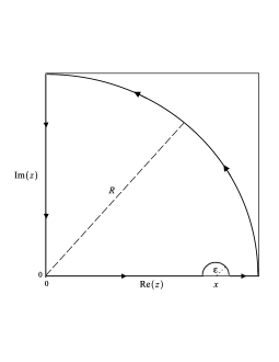
Figure 3: The contour of integration used in Eq. (I).

and using the Cauchy’s integral theorem FWByron92 , we find that

$$\int_{0}^{x}\frac{e^{-y\xi}}{x-y}dy=-\lim_{R\to\infty}\int_{Q_{R}}\frac{e^{-z\xi}}{x-z}dz-\lim_{\varepsilon\to 0}\int_{S_{\varepsilon}}\frac{e^{-z\xi}}{x-z}dz$$

$$\quad-\lim_{R\to\infty}\int_{iR}^{0}\frac{ie^{-ir\xi}}{x-ir}dr-\lim_{R\to\infty}\int_{x}^{R}\frac{e^{-y\xi}}{x-y}dy.$$ (1)

The imaginary part of the integral over the quadrant $Q_{R}$ vanishes. This can be shown by setting $z=Re^{i\theta}$ and studying the integral

$${\rm Im}\left[\lim_{R\to\infty}\int_{Q_{R}}\frac{e^{-z\xi}}{x-z}dz\right]=\lim_{R\to\infty}\int_{0}^{\pi/2}{\rm Im}[\psi(Re^{i\theta})]d\theta,$$ (2)

where $\psi(z)=ize^{-\xi z}/(x-z)$ and ${\rm Im}[\psi(Re^{i\theta})]$ is an even function of $R$ and $\theta$ equals to

$${\rm Im}[\psi(Re^{i\theta})] =\frac{Re^{-R\xi\cos\theta}}{x^{2}-2Rx\cos\theta+R^{2}}[(x\cos\theta-R)$$

$$\times\cos(R\xi\sin\theta)+x\sin\theta\sin(R\xi\sin\theta)].$$ (3)

Observe that Eq. (I) for $\theta=\pi/2$ can be estimated by ${\rm Im}[\psi(iR)]\leq R(x-R)/(x^{2}+R^{2})$ which it is smaller or equal to ${\rm Im}[\psi(R)]$ for $0<x<R$. That leads to

$${\rm Im}[\psi(Re^{i\theta})]\leq{\rm Im}[\psi(R)]=\frac{Re^{-R\xi}}{x-R}.$$

After substituting it into Eq. (2) it can be shown that the imaginary part of integral over the quadrant of radius $R$ goes to zero by choosing $R$ sufficiently large.

We set $x-z=\varepsilon e^{i\phi}$ in the second integral in the right hand side of Eq. (I), so that

$$\lim_{\varepsilon\to 0}\int_{S_{\varepsilon}}\frac{e^{-z\xi}}{x-z}dz =-ie^{-x\xi}\lim_{\varepsilon\to 0}\int_{0}^{\pi}e^{\varepsilon\exp(i\phi)\xi}d\phi$$

$$=-i\pi e^{-x\xi}.$$

The third integral in the r.h.s. of Eq. (I) after changing the variable of integration $ir=y$ and using (ISGradsteyn07, , Eq. (3.352.1) on p. 340) gives the real function

$$\int_{-R}^{0}\frac{e^{-y\xi}}{x-y}dy=e^{-x\xi}\left[{\rm Ei}(R\xi+x\xi)-{\rm Ei}(x\xi)\right],$$

where ${\rm Ei}(x)$ is the exponential integral, see (ISGradsteyn07, , Section 8.2). In the forth integral in the r.h.s. of Eq. (I) we change the variable $z$ as follows $x-z=u$. That gives

$$\int_{x}^{R}\frac{e^{-y\xi}}{x-y}dy=e^{-x\xi}\int_{x-R}^{0}\frac{e^{u\xi}}{u}.$$ (4)

Using the series representation of the exponential it can be shown that Eq. (4) is a real function which goes to infinity for $R\to\infty$. Concluding the considerations we find

$${\rm Im}\left[\int_{0}^{x}\frac{e^{-y\xi}}{x-y}dy\right]=\pi e^{-x\xi}.$$ (5)

References

• (1) W. Götze and L. Sjögren, Relaxation processes in supercooled liquids. Rep. Prog. Phys. 55, No. 3 (1992), 241–376.
• (2) J. C. Phillips, Stretched exponential relaxation in molecular and electronic glasses. Rep. Prog. Phys. 59, No. 9 (1996), 1133–1207.
• (3) C. A. Angell, K. L. Ngai, G. B. McKenna, P. F. McMillan, and S. W. Martin, Relaxation in glassforming liquids and amorphous solids. J. Appl. Phys. 88, No. 6 (2000), 3113–3157.
• (4) L. Cipelletti and L. Ramos, Slow dynamics in glassy soft matter. J. Phys.: Condens. Matter 17, No. 6 (2005), R253–R285.
• (5) L. Pavesi, Influence of dispersive exciton motion on the recombination dynamics in porous silicon. J. Appl. Phys. 80, No. 1 (1996), 216–223.
• (6) I. Mihalcescu, J. C. Vial and R. Romestain, Carrier localization in porous silicon investigated by time-resolved luminescence analysis. J. Appl. Phys. 80, No. 4 (1996), 2404–2410.
• (7) R. Kohlrausch, Theorie des elektrischen Rückstandes in der Leidner Flasche. Pogg. Ann. Chem. 91 (1854) 179–214.
• (8) G. Williams and D. C. Watts, Non-Symmetrical Dielectric Relaxation Behavior Arising from a Simple Empirical Decay Function. Trans. Faraday Soc. 66 (1970) 80–85.
• (9) R. S. Anderssen, S. A. Husain, and R. J. Loy, The Kohlrausch function: properties and applications. ANZIAM J. 45(E) (2004) C800–C816.
• (10) K. Weron and M. Kotulski, On the Cole-Cole relaxation function and related Mittag-Leffler distribution. Physica A 232, No. 1-2 (1996), 180–188.
• (11) J. Sabelko, J. Ervin, and M. Gruebele, Observation of strange kinetics in protein folding. Proc. Natl. Acad. Sci. USA 96, No. 11 (1999), 6031–6036.
• (12) J. Bredenbeck, J. Helbing, J. R. Kumita, G. A. Woolley, and P. Hamm, $\alpha$-Helix formation in a photoswitchable peptide tracked from picoseconds to microseconds by time-resolved IR spectroscopy. Proc. Natl. Acad. Sci. USA 102, No. 7 (2005), 2379–2384.
• (13) J. A. Ihalainen, J. Bredenbeck, R. Pfister, J. Helbing, L. Chi, I. H. M. van Stokkum, G. A. Woolley, and P. Hamm, Folding and unfolding of a photoswitchable peptide from picoseconds to microseconds. Proc. Natl. Acad. Sci. USA 104, No. 13 (2007), 5383–5388.
• (14) Y. Zhang, D. A. Benson, M. M. Meerschaert, and E. M. LaBolle, Space-fractional advection-dispersion equations with variable parameters: Diverse formulas, numerical solutions, and application to the Macrodispersion Experiment site data. Water. Resur. Res. 43 (2007) W05439 (16pp).
• (15) B. Dybiec, E. Gudowska-Nowak, and I. M. Sokolov, Transport in a Lévy ratchet: Group velocity and distribution spread. Phys. Rev. E 78 (2008) 011117 (9pp).
• (16) H. Xi, K.-Z. Gao, J. Ouyang, Y. Shi, and Y. Yang, Slow magnetization relaxation and reversal in magnetic thin films. J. Phys.: Condens. Matter 20, No. 29 (2008), 295220 (8pp).
• (17) A. A. Adjanoh, R. Belhi, J. Vogel, M. Ayadi, and K. Abdelmoula, Compressed exponential form for disordered domain wall motion in ultra-thin Au/Co/Au ferromagnetic films. J. Magn. Magn. Mater. 323, No. 5 (2011), 504–508.
• (18) N. Žurauskiene, S. Balevičius, D. Pavilonis, V. Stankevič, V. Plaušinaitiene, S. Zherlitsyn, T. Herrmannsdörfer, J. M. Law, and J. Wosnitza, Magnetoresistance and Resistance Relaxation of Nanostructured La-Ca-MnO Films in Pulsed Magnetic Fields. IEEE T. Magn. 50, No. 11 (2014), 6100804 (4pp).
• (19) H. Pollard, The representation of $e^{-x^{\lambda}}$ as a Laplace integral. Bull. Amer. Math. Soc. 52 (1946) 908–910.
• (20) H. Bergström, On some expansions of stable distribution functions. Arkiv för Matematik 2, No. 18 (1952), 375–378.
• (21) K. Górska, A. Horzela, K. A. Penson, and G. Dattoli, The higher-order heat-type equations via signed Lévy stable and generalized Airy functions. J. Phys. A: Math. Theor. 46, No. 42 (2013), 425001 (16pp).
• (22) E. Orsingher and M. D’Ovidio, Probabilistic representation of fundamental solutions to $\frac{\partial u}{\partial t}=\kappa_{m}\frac{\partial^{m}u}{\partial x^{m}}$. Elec. Comm. Prob. 17 (2012) article 34.
• (23) J. Klafter and R. Silbey, Derivation of the Continuous-Time Random-Walk Equation. Phys. Rev. Lett. 44, No. 2 (1980), 55–58.
• (24) D. Bedeaux, K. Lakatos-Lindenberg, and K. E. Shuler, On the relation between master equations and random walks and their solutions. J. Math. Phys. 12, No. 10 (1971), 2116–2123.
• (25) V. M. Kenkre, E. W. Montroll, and M. F. Shlesinger, Generalized master equations for continuous-time random walks. J. Stat. Phys. 9, No. 1 (1973), 45–50.
• (26) A. Compte, Stochastic foundations of fractional dynamics. Phys. Rev. E. 53, No. 4 (1996), 4191–4193.
• (27) M. Magdziarz and K. Weron, Anomalous diffusion schemes underlying the stretched exponential relaxation. The role of subordinators. Acta Phys. Pol. B 37, No. 5 (2006), 1617–1625.
• (28) B. Dybiec and E. Gudowska-Nowak, Subordinated diffusion and continuous time random walk asymptotics. Chaos 20, No. 4 (2010), 043129 (9pp).
• (29) A. I. Saichev and G. M. Zaslavsky, Fractional kinetic equations: solutions and applications. Chaos 7, No. 4 (1997), 753–764.
• (30) E. Capelas de Oliveira, F. Mainardi, and J. Vaz Jr, Fractional models of anomalous relaxation based on the Kilbas and Saigo function. Meccanica 49, No. 9 (2014), 2049–2060.
• (31) R. Garra, A. Giusti, F. Mainardi, and G. Pagnini, Fractional relaxation with time-varying coefficient. Fract. Calc. Appl. Anal. 17, No. 2 (2014), 424–439.
• (32) M. M. Meerschaert and A. Sikorskii, Stochastic Models for Fractional Calculus. De Gruyter Studies in Mathematics no. 43, Berlin (2012).
• (33) G. Dattoli, K. Górska, A. Horzela, and K. A. Penson, Photoluminescence decay of silicon nanocrystals and Lévy stable distributions. Phys. Lett. A 378, No. 30-31 (2014), 2201–2205.
• (34) K. Weron, A probabilistic mechanism hidden behind the universal power law for dielectric relaxation: general relaxation equation. J. Phys.: Condens. Matter 3, No. 46 (1991), 9151–9162.
• (35) V. M. Zolotarev, One-dimensional Stable Distributions. Nauka, Moscow (1983), Amer. Math. Soc. Providence, RI (1986).
• (36) K. Górska and K. A. Penson, Lévy stable distributions via associated integral transform. J. Math. Phys. 53, No. 5 (2012), 053302 (10pp).
• (37) K. A. Penson and K. Górska, On the properties of Laplace transform originating from one-sided Lévy stable laws. J. Phys. A: Math. Theor. 49, No. 6 (2016), 065201 (10pp).
• (38) F. Mainardi, G. Pagnini, and R. Gorenflo, Mellin Transform and Subordination Laws in Fractional Diffusion Processes. Fract. Calc. Appl. Anal. 6, No. 4 (2003), 441–459.
• (39) I. N. Sneddon, The Use of Integral Transforms, vol. 2. TATA McGraw-Hill, New Delhi (1974).
• (40) I. S. Gradshteyn and I. M. Ryzhik, Table of Integrals, Series, and Products’, 7th ed., A. Jeffrey and D. Zwillinger (Eds). Academic Press, New York (2007).
• (41) J. Mikusiński, On the function whose Laplace-transform is $e^{-s^{\alpha}}$. Studia Math. 18 (1959) 191–198.
• (42) K. A. Penson and K. Górska, Exact and Explicit Probability Densities for One-Sided Lévy Stable Distributions. Phys. Rev. Lett. 105 (2010) 210604 (4pp).
• (43) A. P. Prudnikov, Yu. A. Brychkov, and O. I. Marichev, Integrals and Series. vol. 3. More Special Functions. Fizmatlit, Moscow (2003).
• (44) K. Górska and K. A. Penson, Lévy stable two-sided distributions: Exact and explicit densities for asymmetric case. Phys. Rev. E 83 (2011) 061125 (4pp).
• (45) W. Feller, An Introduction to Probability Theory and Its Applications, vol. 2. Wiley, New York (1971).
• (46) A. P. Prudnikov, Yu. A. Brychkov, and O. I. Marichev, Integrals and Series, vol. 1. Elementary Functions. Gordon and Breach, Amsterdam (1998).
• (47) F. W. Byron and R. W. Fuller, Mathematics of Classical and Quantum Physics, vol. 2. Dover Publications, New York (1992).
• (48) I. Podlubny, Fractional Differential Equations in Mathematics and Science and Engineering vol. 198. Academic Press, San Diego (1999).
• (49) V. Kiryakova and Y. Luchko, Riemann-Liouville and Caputo type multiple Erdélyi-Kober operators. Cent. Eur. J. Phys. 11, No. 10 (2013), 1314–1336.
• (50) S. G. Samko, A. A. Kilbas, and O. I. Marichev, Fractional Integrals and Derivatives. Theory and Applications. Gordon and Breach Science Publishers, Switzerland (1993).
• (51) F. Mainardi, Y. Luchko, and G. Pagnini, The fundamental solution of the space-time fractional diffusion equation. Fract. Calc. Appl. Anal. 4, No. 2 (2001), 153–192.
• (52) Yu. A. Brychkov and A. P. Prudnikov, Integral Transforms of Generalized Functions. Nauka, Moscow (1977) (in russian).
• (53) F. Mainardi, P. Paradisi, and R. Gorenflo, Probability distributions generated by fractional diffusion equations (2007) arXiv: 0704.0320 (46pp).
• (54) R. Gorenflo and F. Mainardi, Fractional calculus and stable probability distributions. Arch. Mech. 50, No. 3 (1998), 377–388.
• (55) J. S. Lew, On some relations between the Laplace and Mellin Transforms. IBM J. Res. Dev. 19, No. 6 (1975), 582–586.
• (56) K. Górska and W. A. Woyczyński, Explicit representations for multiscale Lévy processes, and asymptotics of multifractal conservation laws. J. Math. Phys. 56, No. 8 (2015), 083511 (19pp).
• (57) F. Oberhettinger, Tables of Mellin Transforms. Springer-Verlag, Berlin (1974).