Adaptive heat engine

Abstract

A major limitations for many heat engines is that their functioning demands on-line control, and/or an external fitting between environmental parameters (e.g. temperatures of thermal baths) and internal parameters of the engine. We study a model for an adaptive heat engine, where—due to feedback from the functional part—the engine’s structure adapts to given thermal baths. Hence no on-line control and no external fitting are needed. The engine can employ unknown resources; it can also adapt to results of its own functioning that makes the bath temperatures closer. We determine thermodynamic costs of adaptation and relate them to the prior information available about the environment. We also discuss informational constraints on the structure-function interaction that are necessary for adaptation.

Introduction. Heat-engines drove the Industrial Revolution and their foundation, viz. thermodynamics, became one of the most successful physical theories callen . Its extensions to stochastic sekimoto ; seifert and quantum domain mahler led to new generations of heat engines seifert ; mahler ; debashish ; scovil ; prokhor ; kosloff ; tannor ; uzdin ; johal ; arm ; pop ; barba ; scully . As everyone could observe, the work-extraction function of macroscopic heat-engines requires external on-line control, e.g. the specific sequence of adiabatic and isothermal processes for the Carnot cycle callen ; kauffman . Smaller engines may not demand on-line control, i.e. they are autonomous pop ; barba , but they do demand fitting between internal and environmental parameters scovil ; prokhor ; kosloff ; tannor ; uzdin ; johal ; arm , e.g. because for fixed environment (thermal baths) there are internal parameters, under which the machine acts as a heat-pump or refrigerator performing tasks just opposite to that of heat-engine. Such fitted engines are susceptible to environmental changes, e.g. when the bath temperatures get closer due to the very engine functioning. Car engines treat this problem by abandoning the partially depleted fuel (i.e. the hot bath), and using fresh fuel.

Here we study a rudimentary model of autonomous, adaptive heat engine. Adaptive means that the engine can work for a sufficiently general class of environments, i.e. it does need neither on-line control, nor an externally imposed fitting between its internal parameters and the bath temperatures. In particular, the engine can adapt to the results of its own functioning.

The major biophysical heat engine, viz photosynthesis—which operates between the hot Sun temperature and the low-temperature Earth environment mex —does have adaptive features that allow its functioning under decreased hot temperature (partial shadowing) or increased cold temperature (hot whether) igor ; adaptive_photo_s . Hence adaptive engines can be useful for fueling devices employing unknown or scarce resources. They are already employed in engineering for photovoltaic engines that can operate under partial shadow adaptive_photo_v .

Recently, several physical models concentrated on adaptive sensors (learning and memorizing environmental changes), adaptive transport models etc igor ; tamar ; kaneko ; sartori ; adaptive ; barato ; bo ; sartori_prl . These studies clarified thermodynamic costs of adaptation scenarios igor ; sartori ; adaptive ; barato ; bo ; sartori_prl . Other research lines related adaptation with (poly)homeostasis gros and models of artificial life kauffman ; virgo .

For analyzing the adaptation and its costs for heat engines, we need a tractable and realistic model that is much simpler than its prototypes in photovoltaics or photosynthesis. The model ought to consist of functional and structural parts. For the former we choose one of the most known models of quantum/stochastic thermodynamics scovil ; prokhor ; kosloff ; tannor ; uzdin .

The functional degree of freedom of the model engine has three states: $i=1,2,3$ scovil ; prokhor ; kosloff ; tannor ; uzdin . Its dynamics is described by a Markov master equation kampen :

$$\dot{p}_{i}\equiv{{\rm d}p_{i}}/{{\rm d}t}={\sum}_{j}[\rho_{i\leftarrow j}p_{j}-\rho_{j\leftarrow i}p_{i}],\quad i,j=1,2,3,$$ (1)

where $p_{i}$ is the probability of $i$, and $\rho_{i\leftarrow j}$ is the transition rate from $j$ to $i$. The stationary solution of (1) is

$$p_{1}=\frac{1}{{\cal Z}}[\rho_{1\leftarrow 2}\rho_{1\leftarrow 3}+\rho_{3\leftarrow 2}\rho_{1\leftarrow 3}+\rho_{2\leftarrow 3}\rho_{1\leftarrow 2}],$$ (2)

$$p_{2}=\frac{1}{{\cal Z}}[\rho_{2\leftarrow 1}\rho_{2\leftarrow 3}+\rho_{3\leftarrow 1}\rho_{2\leftarrow 3}+\rho_{2\leftarrow 1}\rho_{1\leftarrow 3}],$$ (3)

$$p_{3}=\frac{1}{{\cal Z}}[\rho_{3\leftarrow 1}\rho_{3\leftarrow 2}+\rho_{2\leftarrow 1}\rho_{3\leftarrow 2}+\rho_{1\leftarrow 2}\rho_{3\leftarrow 1}],$$ (4)

where ${\cal Z}$ ensures $p_{1}+p_{2}+p_{3}=1$. We assume that each transition $i\leftrightarrow j$ couples with the bath at inverse temperatures $\beta_{ij}=\beta_{ji}$. The detailed balance reads kampen :

$$\rho_{i\leftarrow j}\,e^{-\beta_{ij}E_{j}}=\rho_{j\leftarrow i}\,e^{-\beta_{ij}E_{i}},\qquad\beta_{ij}=\beta_{ji},$$ (5)

where $E_{i}$ is the energy of $i$. One of the baths has infinite temperature: $\beta_{12}=0$. It is standardly associated with a work-source, because due to ${\rm d}S_{12}=\beta_{12}{\rm d}Q_{12}=0$ it exchanges energy ${\rm d}Q_{12}\not=0$ at zero entropy increase ${\rm d}S_{12}=0$. Effectively large temperatures arise naturally in biomolecular systems due to the stored energy, which—when recalculated in terms of temperature—is some 20–50 times larger than the room temperature stored .

The model (1, 5) was introduced and studied in the quantum setting scovil ; prokhor ; kosloff ; tannor ; uzdin , as a model for maser. Closely related models were studied recently in the context of photovoltaic engines scully .

The average energy conservation in the stationary regime reads from (1): $\sum_{k=1}^{3}\dot{p}_{k}E_{k}=J_{31}+J_{32}+J_{21}=0$, where $J_{i>j}$ is the energy current from the bath that drives the transition $i\leftrightarrow j$:

$$J_{i>j}=(E_{i}-E_{j})(\rho_{i\leftarrow j}p_{j}-\rho_{j\leftarrow i}p_{i}).$$ (6)

$J_{i>j}$ is positive when the energy comes out from the bath. Using (2–4) we get in the stationary state

$$J_{21}=\frac{\hat{E}_{2}}{{\cal Z}}\,\rho_{1\leftarrow 3}\,\rho_{3\leftarrow 2}\,\rho_{1\leftarrow 2}\left[1-e^{(\beta_{32}-\beta_{31})\hat{E}_{3}-\beta_{32}\hat{E}_{2}}\right],$$ (7)

$$J_{31}=-{\hat{E}_{3}J_{21}}/{\hat{E}_{2}},~{}~{}J_{32}={(\hat{E}_{3}-\hat{E}_{2})J_{21}}/{\hat{E}_{2}},$$ (8)

$$\hat{E}_{2}\equiv E_{2}-E_{1},\qquad\hat{E}_{3}\equiv E_{3}-E_{1}.$$ (9)

The heat-engine functioning is defined as [cf. (5, 6)]

$$0>J_{21}=(E_{2}-E_{1})(p_{1}-p_{2})\rho_{1\leftarrow 2},$$ (10)

i.e. the energy goes to the work-source. Note that (10) relates to population inversion between energy levels $E_{1}$ and $E_{2}$. Using (7) we write (10) as

$$\hat{E}_{2}[(1-\vartheta)\hat{E}_{3}-\hat{E}_{2}]>0,\quad\vartheta\equiv\beta_{31}/\beta_{32}.$$ (11)

Eq. (11) demands different temperatures: $\beta_{32}\not=\beta_{31}$. It also demands tuning between the energies $\hat{E}_{2}$, $\hat{E}_{3}$ and $\vartheta$: it is impossible to hold (11) for a wide range of $\vartheta$ by means of constant $\hat{E}_{2}$ and $\hat{E}_{3}$; e.g. if (11) holds for $1>\vartheta$ due to $\hat{E}_{3}>\hat{E}_{2}>0$, then it is violated for $1-\vartheta<\frac{\hat{E}_{2}}{\hat{E}_{3}}$. Tuning is necessary, since for suitable values of $\hat{E}_{2}$ and $\hat{E}_{3}$, the machine can function also as a refrigerator (i.e. $J_{21}>0$ and $J_{32}>0$ for $\beta_{32}>\beta_{31}$) or as a heat-pump.

The structural degree of freedom $x$ is continuous, since it should ensure adaptation to continuous environmental variations. $x$ governs the behavior of interaction energies $E_{i}(x)$ between $x$ and $i$. The joint probability $p_{i}(x,t)$ of $x$ and $i$, $\int{\rm d}x\sum_{i}p_{i}(x,t)=1$, evolves via the Fokker-Planck plus master equations [cf. (1)] kampen :

$$\dot{p}_{i}(x,t) = {\sum}_{j}[\rho_{i\leftarrow j}(x)p_{j}(x,t)-\rho_{j\leftarrow i}(x)p_{i}(x,t)]~{}~{}~{}~{}$$ (12)

$$+ \frac{1}{\gamma}\partial_{x}[p_{i}(x,t)E^{\prime}_{i}(x)]+D\partial^{2}_{x}p_{i}(x,t),$$ (13)

where $i,j=1,2,3$, $E^{\prime}_{i}(x)\equiv\frac{{\rm d}E_{i}(x)}{{\rm d}x}$, $\gamma>0$ is the damping constant, and $D>0$ is the diffusion constant. $\rho_{i\leftarrow j}(x)$ is specified in (19); it holds (5) with $E_{i}\to E_{i}(x)$ and $E_{j}\to E_{j}(x)$.

Eqs. (12, 13) is well-known in chemical and biological applications zwanzig ; hans ; leh ; agmon_h ; blum ; conformon ; christo . The limit when $E_{i}(x)=E(x)$ does not depend on $i$ refers to a dynamic disorder zwanzig ; hans ; leh ; agmon_h . It was applied to a variety of problems including the conformational dynamics of enzymes and ion channels zwanzig ; hans ; leh ; agmon_h . These systems also provide examples, where the dependence of $E_{i}(x)$ on $i$ (feedback) is essential leh ; blum ; conformon ; christo .

We assume in (12) that $x$ is slow: $\frac{1}{\gamma},\,D\ll\rho_{i\leftarrow j}(x)$. This limit is implemented by introducing in (13, 12) the conditional probability $p_{i|x}(t)$ a+n ,

$$p_{i}(x,t)=p_{i|x}(t)p(x,t),\,\int{\rm d}x\,p(x,t)=1,\,\sum_{i}p_{i|x}(t)=1,$$

and collecting fast terms:

$$\dot{p}_{i|x}={\sum}_{j}[\rho_{i\leftarrow j}(x)p_{j|x}-\rho_{j\leftarrow i}(x)p_{i|x}].$$ (14)

Slow terms are found from (13, 14) by summing over $i$:

$$\dot{p}(x,t)=\frac{1}{\gamma}\partial_{x}[p(x,t)\sum_{i}p_{i|x}E^{\prime}_{i}(x)]+D\partial^{2}_{x}p(x,t).$$ (15)

Since $i$ is fast, $p_{i|x}$ in (15) can be taken as time-independent, i.e. $p_{i|x}$ is found from (2–4) upon replacing there $\rho_{ij}\to\rho_{ij}(x)$ a+n . The stationary probability of $x$ is found from (15) via the zero-current condition $\frac{p(x)}{\gamma}\sum_{i}p_{i|x}E^{\prime}_{i}(x)+D\partial_{x}p(x)=0$:

$$p(x)\propto e^{-\Psi(x)/(\gamma D)},\quad\Psi^{\prime}(x)\equiv{\sum}_{i=1}^{3}p_{i|x}E^{\prime}_{i}(x),$$ (16)

where $\Psi(x)$ is an effective potential of $x$, and $\Psi^{\prime}(x)=\frac{{\rm d}\Psi}{{\rm d}x}$.

Adaptation. Naturally, the energies $E_{i}(x)$ do not depend on $\beta_{31}$ and $\beta_{32}$. We choose $E_{i}(x)$ such that two conditions hold. First, $\Psi(x)$ has a unique minimum $\hat{x}$:

$$\Psi^{\prime}(\hat{x})={\sum}_{i=1}^{3}p_{i|\hat{x}}E^{\prime}_{i}(\hat{x})=0,\quad\Psi^{\prime\prime}(\hat{x})>0.$$ (17)

$\hat{x}$ is the unique maximally probable value of $x$; cf. (16).

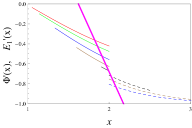
Figure 1: $\Phi^{\prime}(x)$ given by (20, 19) with $f[y,\beta]=e^{y/2}$ for varying $\beta_{31}$ and fixed $\beta_{32}=1$ (first type of varying environment). We assume $\hat{E}_{3}(x)=-x$, $\hat{E}_{2}(x)=x-2$, and (18) holds for $x>2$ if $\vartheta>2$, for $\frac{2}{2-\vartheta}>x>2$ if $1<\vartheta<2$, and for $\frac{2}{2-\vartheta}<x<2$ if $\vartheta<1$. $\Phi^{\prime}(x)$ is shown for various $\vartheta=\beta_{31}/\beta_{32}$ and those $x$ that support (18): $\vartheta=0.1$ (red curve), $\vartheta=0.25$ (green), $\vartheta=0.5$ (blue), $\vartheta=0.75$ (brown), $\vartheta=0.95$ (black), $\vartheta=1.2$ (black-dashed), $\vartheta=1.5$ (brown-dashed), $\vartheta=2.5$ (blue-dashed). The magenta curve shows $-E_{1}^{\prime}(x)$, where $E_{1}^{\prime}(x)=1.8(x-2)+0.680289$. Intersections of $-E_{1}^{\prime}(x)$ with $\Phi^{\prime}(x)$ determine $\hat{x}$. Eqs. (21) hold for all $\vartheta$.

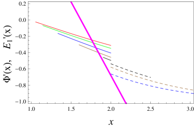
Figure 2: The same as in Fig. 1, but for $\beta_{32}=0.7$. It is seen that for $\vartheta$ close to $1$, no heat-engine functioning exists ((18) does not hold), i.e. the magenta curve does not cross the curves with $\vartheta=0.95$, $\vartheta=1.2$ and $\vartheta=1.5$.

Second, the heat-engine condition $J_{21}(x)<0$ holds in a vicinity of the maximally probable value $\hat{x}$ [cf. (11)]:

$$\hat{E}_{2}(x)[(1-\vartheta)\hat{E}_{3}(x)-\hat{E}_{2}(x)]>0,~{}~{}x\simeq\hat{x},$$ (18)

where $\hat{E}_{i}(x)=E_{i}(x)-E_{1}(x)$; cf. (9). Eqs. (17, 18) imply feedback adaptation: if $\beta_{31}$ or $\beta_{32}$ change, the system is not anymore in a stationary state. It then goes to new stationary state, where the heat-engine function most probably holds.

Note that $x$ is continuous, because we shall assume that $\beta_{31}$ and $\beta_{23}$ change in continuous domains. Using here a feed-forward (instead of feedback) control does not lead to adaptation, because it influences only the diffusion constant $D$; see sect. 1 of suppl. material.

To get a general method for studying (17, 18), we focus on the following class of transition rates $\rho_{ij}$ [cf. (1, 5)]:

$$\rho_{ij}(x)=f[\,\beta_{ij}(E_{j}(x)-E_{i}(x)),\beta_{ij}\,],~{}~{}~{}\beta_{ij}=\beta_{ji},$$ (19)

where $f[y,\beta]$ holds (5). Eq. (19) implies that $\rho_{ij}(x)$ and the stationary probabilities $p_{i|x}$ depend only on $\hat{E}_{3}(x)$ and $\hat{E}_{2}(x)$; cf. (19, 9). This holds in the high-temperature limit for any $\rho_{ij}$; see (5). Two other examples of (19) is the Kramers’ rate $f[y,\beta]=e^{\beta\delta+{\rm min}(y,0)}$, where $\delta$ is the barrier height kampen , and $f[y,\beta]=e^{y/2}$ that corresponds to the discrete-space Fokker-Planck equation agmon_h . We use $\sum_{i=1}^{3}p_{i|x}=1$ and define from (17, 19)

$$\Phi^{\prime}(x)={\sum}_{i=2}^{3}p_{i|x}\hat{E}^{\prime}_{i}(x),$$ (20)

where the analogues of (17) read

$$\Phi^{\prime}(\hat{x})=-E^{\prime}_{1}(\hat{x}),\qquad\Phi^{\prime\prime}(\hat{x})>-E^{\prime\prime}_{1}(\hat{x}).$$ (21)

For given $\hat{E}_{3}(x)$ and $\hat{E}_{2}(x)$, $\Phi^{\prime}(x)$ does not depend on $E_{1}(x)$; see (2–4). Hence one can study $\Phi^{\prime}(x)$ for given $\hat{E}_{3}(x)$ and $\hat{E}_{2}(x)$ [cf. (18)] and for different values of $\beta_{31}$ and $\beta_{32}$. Then one can define $\hat{x}$ via (21) by choosing a suitable $E_{1}(x)$ that does not depend on $\beta_{31}$ and on $\beta_{32}$.

Since (18) should hold for $\vartheta\to 1$, there exists $x_{0}$ such that $\hat{x}\to x_{0}$ for $\vartheta\to 1$, and $\hat{E}_{2}(x_{0})=0$. In the vicinity of $x_{0}$, $\hat{E}_{3}(x)$ is either finite or goes to zero slower than $\hat{E}_{2}(x)$, so that (18) still holds for $\vartheta\to 1$ and $\hat{x}\to x_{0}$.

Let us first assume that one temperature (say $\beta_{31}$) takes arbitrary positive values, while another one ($\beta_{32}$) is fixed. Adaptation is necessary here, since $\vartheta=\beta_{31}/\beta_{32}$ is an arbtrary positive number, hence (18) cannot be valid for $x$-independent $E_{i}$. Now (17, 18) for adaptation can be satisfied; see Fig. 1 for the simplest but representative choice, where $E_{i}(x)$ are parabolic functions of $x$. This choice of $E_{i}(x)$ is realistic leh ; blum ; conformon ; christo .

Since the validity domain (18) of the heat-engine shrinks to a point for $\vartheta\to 1$, we need progressively smaller values of $D\gamma$ in (16) for ensuring the average work-extraction

$$\langle J_{21}\rangle\equiv\int{\rm d}x\,p(x)\,J_{21}(x)<0$$ (22)

for $\vartheta\to 1$. If the diffusion of $x$ is caused by an equilibrium bath, we get $D\gamma=T$ kampen , and the temperature $T$ of this bath should be sufficiently low for (22) to hold. If this is the lowest temperature, there is a heat current towards it tending to increase it. Hence this low temperature is a thermodynamic resource. For a given $D\gamma$, there is a vicinity of $\vartheta=1$, where no work is extracted in average: $\langle J_{21}\rangle>0$.

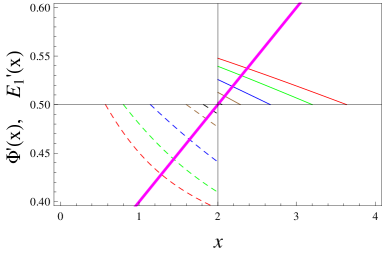
Figure 3: Adaptation for a negative friction $\gamma<0$, $\beta_{32}=1$ and varying $\beta_{13}$. The same parameters as in Fig. 1, but now $\hat{E}_{3}(x)=x/2$. Conditions (18) amount to $\frac{4}{1+\vartheta}>x>2$ if $\vartheta<1$, and to $\frac{4}{1+\vartheta}<x<2$ if $\vartheta>1$. $\Phi^{\prime}(x)$ is shown for: $\vartheta=0.1$ (red curve), $\vartheta=0.25$ (green), $\vartheta=0.5$ (blue), $\vartheta=0.75$ (brown), $\vartheta=0.95$ (black), $\vartheta=1.2$ (black-dashed), $\vartheta=1.5$ (brown-dashed), $\vartheta=2.5$ (blue-dashed), $\vartheta=4$ (green-dashed), $\vartheta=6$ (red-dashed). The magenta curve shows $-E_{1}^{\prime}(x)$, where $E_{1}^{\prime}(x)=-0.1(x-2)-0.5$. Eq. (23) holds.

Consider now a general situation, where both $\beta_{31}$ and $\beta_{32}$ vary. Fig. 2 shows that the set-up which worked for a fixed $\beta_{32}$ does not apply here. Now condition $\Phi^{\prime}(\hat{x})=-E^{\prime}_{1}(\hat{x})$ in (21) implies such a behavior for $\Phi^{\prime}(\hat{x})$ under $\beta_{31}\approx\beta_{32}$ that the second condition $\Phi^{\prime\prime}(\hat{x})>-E^{\prime\prime}_{1}(\hat{x})$ in (21) cannot hold; e.g. because $\Phi^{\prime}(\hat{x})$ has the shape shown in Figs. 3 and 4. This fact is shown in sect. 2 of suppl. material. The only possibility to recover the adaptive heat engine function is to assume that $x$ is subject to an external force that adds to RHS of (15) a contribution making the effective friction negative: $\gamma<0$. Then $D\gamma<0$ in (16), and the most probable $\hat{x}$ means that inequalities in (17) and (21) are reversed. Now the adaptation conditions are (18) and [instead of (21)]

$$\Phi^{\prime}(\hat{x})=-E^{\prime}_{1}(\hat{x}),\qquad\Phi^{\prime\prime}(\hat{x})<-E^{\prime\prime}_{1}(\hat{x}).$$ (23)

These conditions can be satisfied, as illustrated in Figs. 3 and 4. Now $x$ should change in a bounded domain; otherwise for the natural shape of energies ($E_{i}(x)\to\infty$ for $x\to\pm\infty$) one gets a non-normalizable $p(x)$ in (16). Note that for $\gamma<0$ and $D>0$, (15) does predict relaxation to (16), i.e. the negative-friction situation is stable. The external force that simulates the negative friction does dissipate energy with a constant rate $\Pi=\frac{1}{|\gamma|}\int{\rm d}x\,p(x)[\Psi^{\prime}(x)]^{2}$; see sect. 3 of suppl. material. We still demand a sufficiently small $|\gamma|D$ to ensure $\langle J_{21}\rangle<0$. For a small $|\gamma|D$ we get $\Pi\simeq|\Psi^{\prime\prime}(\hat{x})|D$. This energy dissipation is another cost for adaptation; see sartori ; adaptive ; barato ; bo ; sartori_prl for related results. A negative friction is known in several classes of active (non-equilibrium) systems samo ; wiki ; starr ; brown . Two examples relevant to our situation is the negative resistance of electric circuits wiki and negative viscosity of driven fluids starr .

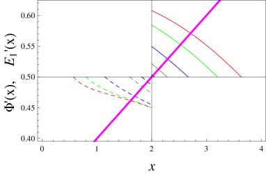
Figure 4: The same as in Fig. 3, but for $\beta_{32}=3$. Eqs. (23, 18) hold.

Above examples of adaptation are obtained for $E_{i}$ being correlated random variables, $P(E_{1},E_{2},E_{3})=\int{\rm d}x\,p(x)\prod_{k=1}^{3}\delta(E_{k}-E_{k}(x))$, and for specific forms of $E_{i}(x)$. To see why such assumptions are necessary, take an extreme case, where the probability density of energies $\Pi(E_{1},E_{2},E_{3})$ is non-informative in terms of the Bayesian statistics jaynes ; johal . Since we do not have prior expectations about correlations between random variables $E_{1}$, $E_{2}$ and $E_{3}$, they are taken as independent $\Pi(E_{1},E_{2},E_{3})=\prod_{k=1}^{3}\Pi(E_{k})$ jaynes . Also, since $E_{1}$ can assume either sign, the non-informative density $\Pi(E_{k})$ is the homogeneous one: $\Pi(E_{k})={\rm const}$ jaynes . Employing this density we calculate from (11) that the probability of the heat-engine functioning is low $\frac{1-{\rm min}(\vartheta,\frac{1}{\vartheta})}{3}<\frac{1}{3}$. Hence the current $J_{21}$ averaged over $\Pi(E_{1},E_{2},E_{3})$ is positive, i.e. the machine does not function as a heat-engine; cf. (7). Thus the coupling between structure and function, which is encoded in $P(E_{1},E_{2},E_{3})$ must be informative.

In sum, we studied a model for an adaptive heat engine that can function under scarce or unknown resources. Several physical limitations for the adaptation concept were uncovered; they relate to the prior information available about the environment. One problem generated by this research is that in the model the resources needed for adaptation are detached from the work extracted by the engine. Employing the extracted work for ensuring the adaptation will make the situation more interesting.

This work is partially supported by COST MP1209 and by the ICTP through the OEA-AC-100.

I Supplementary material

I.1 1. Feed-forward control

Feed-forward amounts to no direct interaction between the functional degree of freedom $i$ and the structural degree of freedom $x$. But now $x$ couples directly to the baths at temperatures $T_{31}=1/\beta_{31}$ and $T_{32}=1/\beta_{32}$, i.e. we try to implement temperature sensors via $x$. This means taking in (13) of the main text $E_{i}(x)=E(x)$ and adding there the following term

$$\sum_{\alpha={31,32}}\gamma^{-1}_{\alpha}[\partial_{x}[p_{i}(x,t)E^{\prime}(x)]+T_{\alpha}\partial^{2}p_{i}(x,t)].$$ (24)

Instead of (16) [of the main text] we get for the stationary probability

$$\bar{p}(x)\propto e^{-E(x)/\widetilde{D}},\qquad\widetilde{D}=\frac{D+\sum_{\alpha={31,32}}\gamma^{-1}_{\alpha}T_{\alpha}}{\gamma^{-1}+\sum_{\alpha={31,32}}\gamma^{-1}_{\alpha}},$$ (25)

where $E(x)$ does not depend on $\beta_{31}$ and $\beta_{32}$. Hence no adaptation is possible.

I.2 2. Derivation of the no-adaptation condition

If both $\beta_{31}$ and $\beta_{32}$ can vary, the adaptation condition $\Phi^{\prime}(\hat{x})=-E^{\prime}_{1}(\hat{x})$ [see (21) of the main text] should hold for all $\beta_{31}$ and $\beta_{32}$. In particular, this means that—since $E_{1}^{\prime}(x)$ does not depend on $\beta_{31}$ and $\beta_{32}$— $\Phi^{\prime}(x_{0})\left|{}_{\beta_{31}=\beta_{32}=\beta}\right.$ should not depend on $\beta_{31}=\beta_{32}=\beta$, where $\hat{E}_{2}(\hat{x}=x_{0})=0$. Now (2–4) of the main text show that $p_{i|x_{0}}$ are at equilibrium for $\beta_{31}=\beta_{32}=\beta$ and

$$p_{1|x_{0}}=p_{2|x_{0}}=\frac{1}{Z},\qquad p_{3|x_{0}}=\frac{e^{-\beta\hat{E}_{3}}}{Z}.$$ (26)

Hence we get

$$\Phi^{\prime}(x_{0})\left|{}_{\beta_{32}=\beta_{31}=\beta}\right.=\frac{\hat{E}_{2}^{\prime}(x_{0})+\hat{E}_{3}^{\prime}(x_{0})e^{-\beta\hat{E}_{3}(x_{0})}}{2+e^{-\beta\hat{E}_{3}(x_{0})}}.$$ (27)

This expression is not a function of $\beta$ only for

$$\hat{E}_{2}^{\prime}(x_{0})=2\hat{E}_{3}^{\prime}(x_{0}),$$ (28)

where

$$\Phi^{\prime}(x_{0})\left|{}_{\beta_{31}=\beta_{32}=\beta}\right.=\hat{E}_{3}^{\prime}(x_{0}).$$ (29)

Using (28) we find $\Phi^{\prime}(x)$ for $x\approx x_{0}$:

$$\Phi^{\prime}(x)=\Phi^{\prime\prime}(x_{0})(x-x_{0})+\hat{E}_{2}^{\prime}(x_{0})p_{2|x_{0}}+\hat{E}_{3}^{\prime}(x_{0})p_{3|x_{0}}$$

$$=\Phi^{\prime\prime}(x_{0})(x-x_{0})+\hat{E}_{3}^{\prime}(x_{0})+\hat{E}_{3}^{\prime}(x_{0})[p_{2|x_{0}}-p_{1|x_{0}}].$$ (30)

We shall focus on the last term in (30) that determines the shape of $\Phi^{\prime}(x)$ as a function of $\beta_{31}$ and $\beta_{32}$. This term is expanded for $\beta_{31}\approx\beta$, $\beta_{32}\approx\beta$:

$$b\equiv\hat{E}_{3}^{\prime}(x_{0})[p_{2|x_{0}}-p_{1|x_{0}}]$$

$$=\hat{E}_{3}^{\prime}(x_{0}){\sum}_{\alpha={31},{32}}(\beta_{\alpha}-\beta)\partial_{\beta_{\alpha}}[p_{2|x_{0}}-p_{1|x_{0}}].$$ (31)

To work out (31) via (2–4) of the main text, we shall assume for the transition rates $\rho_{i\leftarrow j}$:

$$\rho_{ij}(x)=f_{ij}[\,\beta_{ij}(E_{j}(x)-E_{i}(x)),\beta_{ij}\,],~{}~{}~{}\beta_{ij}=\beta_{ji},$$ (32)

where $f_{ij}[y,\beta]$ holds the detailed balance conditions; see (5) of the main text. Eq. (32) is more general than its analogue (19) in the main text. Combining (31) with (32) and with (2–4) of the main text, we get

$$p_{2|x_{0}}-p_{1|x_{0}}=\frac{1}{Z(x_{0})}[f_{32}(\beta_{32}\hat{E}_{3}(x_{0}))f_{31}(-\beta_{31}\hat{E}_{3}(x_{0}))-$$

$$f_{31}(\beta_{31}\hat{E}_{3}(x_{0}))f_{32}(-\beta_{32}\hat{E}_{3}(x_{0}))\,],$$ (33)

$$b=\frac{\hat{E}_{3}(x_{0})\hat{E}_{3}^{\prime}(x_{0})}{Z(x_{0})}{\sum}_{\alpha={31,32}}(\beta-\beta_{\rm\alpha})\psi_{\alpha}[\beta\hat{E}_{3}(x_{0})],$$ (34)

where we denoted $f^{\prime}_{ij}[y,\beta]\equiv\partial_{y}f_{ij}[y,\beta]$,

$$\psi_{31}[x]\equiv f^{\prime}_{31}[x,\beta]f_{32}[-x,\beta]+f^{\prime}_{31}[-x,\beta]f_{32}[x,\beta],$$ (35)

$$\psi_{32}[x]\equiv-f^{\prime}_{32}[-x,\beta]f_{31}[x,\beta]-f^{\prime}_{32}[x,\beta]f_{31}[-x,\beta].$$

Now note the following inequality

$$f^{\prime}_{ij}[y,\beta]=\partial_{y}f_{ij}[y,\beta]\geq 0.$$ (36)

It means that the transition from a lower energy to a higher energy is facilitated, if the lower energy increases or the higher energy decreases. This inequality does follow from the detailed balance [see (5) of the main text], but it still holds for all physical examples we are aware of. The inequality implies $\psi_{\rm 31}[\beta\hat{E}_{3}(x_{0})]\geq 0$ and $\psi_{\rm 32}[\beta\hat{E}_{3}(x_{0})]\leq 0$. Choosing $\beta$ in between of $\beta_{31}$ and $\beta_{32}$ we see that

$${\rm sign}[b]={\rm sign}[\hat{E}_{3}(x_{0})\hat{E}_{2}^{\prime}(x_{0})(1-\vartheta)]$$ (37)

Working out the heat-engine condition [see (18) of the main text] in the considered order ${\cal O}(|1-\vartheta|)$ and ${\cal O}(|x-x_{0}|)$ we obtain

$${\hat{E}_{3}(x_{0})(1-\vartheta)}\left/{\hat{E}_{2}^{\prime}(x_{0})}\right.>x-x_{0}>0,\quad{\rm or}$$ (38)

$${\hat{E}_{3}(x_{0})(1-\vartheta)}\left/{\hat{E}_{2}^{\prime}(x_{0})}\right.<x-x_{0}<0.$$ (39)

Conditions (37–39) imply that depending on the sign of $\Phi^{\prime\prime}(x_{0})$ in (30), $\Phi^{\prime}(x)$ can assume in the vicinity of $x_{0}$ only two possible shapes; one of them is shown in Figs. 3 and 4 of the main text. Obviously, neither of them is compatible with $\Phi^{\prime\prime}(\hat{x})>-E^{\prime\prime}_{1}(\hat{x})$; see (21) of the main text.

I.3 3. Energy dissipation due to external force that generates negative friction

Consider (15, 16) of the main text that we generalize as follows:

$$\dot{p}(x,t)=\frac{1}{\gamma}\partial_{x}[p(x,t)\Psi^{\prime}(x)]+\frac{T}{\gamma}\partial^{2}_{x}p(x,t)$$ (40)

$$+\partial_{x}[p(x,t)G^{\prime}(x)],$$ (41)

where we assume that $x$ couples with a thermal bath at temperature $T$,

$$\gamma>0,$$ (42)

is the friction constant, and $G^{\prime}(x)=\frac{{\rm d}}{{\rm d}x}G(x)$ is an external force. If now we set

$$G(x)=-\frac{2}{\gamma}\Psi(x),$$ (43)

the resulting influence of $G(x)$ and $\Psi(x)$ is equivalent to a negative friction.

The average energy $\Pi$ dissipated per unit of time due to the external force $G^{\prime}(x)$ can be estimated via the change of the free energy

$$F=\int{\rm d}x\,p(x,t)[\Psi(x)+T\ln p(x,t)],$$ (44)

of $x$ due to the external part (41) of the dynamics

$$\Pi=\int{\rm d}x\,\partial_{x}[p(x,t)G^{\prime}(x)]\,[\Psi(x)+T\ln p(x,t)].$$ (45)

In the stationary state:

$$\Pi=-\int{\rm d}x\,p(x)G^{\prime}(x)\,[\Psi^{\prime}(x)+T\frac{{\rm d}}{{\rm d}x}\ln p(x)]$$ (46)

$$=\gamma\int{\rm d}x\,p(x)[G^{\prime}(x)]^{2},$$ (47)

where $p(x)\propto\exp[-(\Psi(x)+\gamma G(x))/T]$. Using (43) we finally obtain:

$$\Pi=\frac{1}{\gamma}\int{\rm d}x\,p(x)[\Psi^{\prime}(x)]^{2}.$$ (48)

References

(1) H.B. Callen, Thermodynamics and an introduction
to thermostatistics (John Wiley & Sons, NY, 1985).
(2)
K. Sekimoto, Stochastic Energetics (Springer-Verlag, Berlin 2010).
(3) U. Seifert, Rep. Prog. Phys. 75, 126001
(2012).
(4) G. Mahler, Quantum Thermodynamic Processes (Pan
Stanford, Singapore, 2015).
(8) E. Geva and R. Kosloff, Phys. Rev. E 49, 3903 (1994).
(9)E. Boukoza and D. Tannor, Phys. Rev. Lett., 98,
240601 (2007).
(10) R. Uzdin, A. Levy, and R. Kosloff, Phys. Rev. X 5,
031044 (2015).
(11) G. Thomas and R.S. Johal, Phys. Rev. E 85,
041146 (2012).
(12)
A. E. Allahverdyan, K. V. Hovhannisyan, A. V. Melkikh,
and S. G. Gevorkian, Phys. Rev. Lett. 109, 248903 (2013).
(13) N. Linden, S. Popescu, and P Skrzypczyk,
arxiv.1010.6029.
(14) A.S.L. Malabarba, A.J. Short, and P. Kammerlander,
New J. Phys. 17, 045027 (2015).
M.F. Frenzel, D. Jennings, and T. Rudolph, New J. Phys. 18,
023037 (2016).
(15) M.O. Scully, Phys. Rev. Lett. 104, 207701
(2010). M.O. Scully et al., PNAS, 108, 15097 (2011).
(16) S. Kauffman, Phil. Trans. R. Soc. A 361, 1089
(2003).
(17)
E. Albarran-Zavala and F. Angulo-Brown,
Entropy, 9, 152 (2007).
(18) I. Rojdestvenski, M. G. Cottam, G. Oquist,
and N. Huner, Physica A 320, 318 (2003).
(19) S. Falk et al., Photosynthetic
adjustment to temperature, in Photosynthesis and the
environment, pp. 367-385, ed. by N.R. Baker (Springer,
Netherlands, 1996).
(20) D. La Manna et al., Renewable and
Sustainable Energy Reviews, 33, 412 (2014).
(21)
T. Friedlander and N. Brenner, PNAS, 106, 22558 (2009).
(22)
M. Inoue and K. Kaneko, Phys. Rev. E 81, 026203 (2010).
(23)
G. Lan, P. Sartori, S. Neumann, V. Sourjik, Y. Tu,
Nature Phys. 8. 422 (2012).
(24)
A. E. Allahverdyan and Q.A. Wang, Phys. Rev. E 87, 032139
(2013).
(25)
A. C. Barato, D. Hartich, and U. Seifert,
Phys. Rev. E 87, 042104 (2013).
New J. Phys. 16, 103024 (2014).
(26) S. Bo, M. Del Giudice, and A. Celani,
JSTAT, P01014 (2015).
(27) P. Sartori and Y. Tu, Phys. Rev. Lett. 115, 118102 (2015).
(28)
D. Markovic and C. Gros, Phys. Rev. Let. 105, 068702 (2010).
(29) S. McGregor and N. Virgo, in Advances in
Artificial Life: Darwin Meets von Neumann, pp. 230-237 (Springer,
Berlin, 2009).
(30)N.G. van Kampen, Stochastic Processes in Physics
and Chemistry (Elsevier, Amsterdam, 2007).
(31)
C.W.F. McClare, J. Theor. Biol. 35, 233 (1972).
E.T. Jaynes, The muscle as an engine (1983),
http://bayes.wustl.edu/etj/articles/muscle.pdf
(41)V.P. Starr, Physics of negative viscosity
phenomena (McGraw-Hill, 1968).
(42)B. Cleuren and C. Van den Broeck, Phys. Rev. E. 65, 030101(R) (2002). A. Haljas, R. Mankin, A. Sauga, E. Reiter,
Phys. Rev. E. 70, 041107. (2004). J. Spiechowicz, J. Luczka,
P. Hanggi, JSTAT P02044 (2013).
(43) A.E. Allahverdyan and Th.M. Nieuwenhuizen, Phys. Rev. E,
62, 845 (2000).