Fast Dpp Sampling for Nyström
with Application to Kernel Methods

Abstract

The Nyström method has long been popular for scaling up kernel methods. Its theoretical guarantees and empirical performance rely critically on the quality of the landmarks selected. We study landmark selection for Nyström using Determinantal Point Processes (Dpps), discrete probability models that allow tractable generation of diverse samples. We prove that landmarks selected via Dpps guarantee bounds on approximation errors; subsequently, we analyze implications for kernel ridge regression. Contrary to prior reservations due to cubic complexity of Dpp sampling, we show that (under certain conditions) Markov chain Dpp sampling requires only linear time in the size of the data. We present several empirical results that support our theoretical analysis, and demonstrate the superior performance of Dpp-based landmark selection compared with existing approaches.

1 Introduction

Low-rank matrix approximation is an important ingredient of modern machine learning methods. Numerous learning tasks rely on multiplication and inversion of matrices, operations that scale cubically in the number of data points $N$, and therefore quickly become a bottleneck for large data. In such cases, low-rank matrix approximations promise speedups with a tolerable loss in accuracy.

A notable instance is the Nyström method [32, 43], which takes a positive semidefinite matrix $K\in\mathbb{R}^{N\times N}$ as input, selects from it a small subset $C$ of columns $K_{\cdot,C}$, and constructs the approximation $\tilde{K}=K_{\cdot,C}K_{C,C}^{\dagger}K_{C,\cdot}$. The matrix $\tilde{K}$ is then used in place of $K$, which can decrease runtimes from $\mathcal{O}(N^{3})$ to $\mathcal{O}(N|C|^{3})$, a huge savings (since typically $|C|\ll N$).

Since its introduction into machine learning, the Nyström method has been applied to a wide spectrum of problems, including kernel ICA [6, 36], kernel and spectral methods in computer vision [8, 18], manifold learning [39, 40], regularization [35], and efficient approximate sampling [1]. Recent work [12, 5, 2] shows risk bounds for Nyström applied to various kernel methods.

The most important step of the Nyström method is the selection of the subset $C$, the so-called landmarks. This choice governs the approximation error and subsequent performance of the approximated learning methods [12]. The most basic strategy is to sample landmarks uniformly at random [43]. More sophisticated non-uniform selection strategies include deterministic greedy schemes [37], incomplete Cholesky decomposition [17, 7], sampling with probabilities proportional to diagonal values [14] or to column norms [15], sampling based on leverage scores [19], via K-means [44], or using submatrix determinants [9].

We study landmark selection using Determinantal Point Processes (Dpp), discrete probability models that allow tractable sampling of diverse non-independent subsets [31, 26]. Our work generalizes the determinant based scheme of Belabbas and Wolfe [9]. We refer to our scheme as Dpp-Nyström, and analyze it from several perspectives.

A key quantity in our analysis is the error of the Nyström approximation. Suppose $k$ is the target rank; then for selecting $c\geq k$ landmarks, Nyström’s error is typically measured using the Frobenius or spectral norm relative to the best achievable error via rank-$k$ SVD $K_{k}$; i.e., we measure

$${\|K-K_{\cdot,C}K_{C,C}^{\dagger}K_{C,\cdot}\|_{F}\over\|K-K_{k}\|_{F}}\quad\text{ or }\quad{\|K-K_{\cdot,C}K_{C,C}^{\dagger}K_{C,\cdot}\|_{2}\over\|K-K_{k}\|_{2}}.$$

Several authors also use additive instead of relative bounds. However, such bounds are very sensitive to scaling, and become loose even if a single entry of the matrix is large. Thus, we focus on the above relative error bounds.

First, we analyze this approximation error. Previous analyses [9] fix a cardinality $c=k$; we allow the general case of selecting $c\geq k$ columns. Our relative error bounds rely on the properties of characteristic polynomials. Empirically, Dpp-Nyström obtains approximations competitive to state-of-the-art methods.

Second, we consider its impact on kernel methods. Specifically, we address the impact of Nyström-based kernel approximations on kernel ridge regression. This task has been noted as the main application in [5, 2]. We show risk bounds of Dpp-Nyström that hold in expectation. Empirically, it achieves the best performance among competing methods.

Third, we consider the efficiency of Dpp-Nyström; specifically, its tradeoff between error and running time. Since its proposal, determinantal sampling has so far not been used widely in practice due to valid concerns about its scalability. We consider a Gibbs sampler for $k$-Dpp, and analyze its mixing time using a path coupling [11] argument. We prove that under certain conditions the chain is fast mixing, which implies a linear running time for Dpp sampling of landmarks. Empirical results indicate that the chain yields favorable results within a small number of iterations, and the best efficiency-accuracy traedoffs compared to state-of-art methods (Figure 6).

2 Background and Notation

Throughout, we are approximating a given positive semidifinite (PSD) matrix $K\in\mathbb{R}^{N\times N}$ with eigendecomposition $K=U\Lambda U^{\top}$ and eigenvalues $\lambda_{1}\geq\ldots\geq\lambda_{N}$. We use $K_{i,\cdot}$ for the $i$-th row and $K_{\cdot,j}$ for the $j$-th column, and, likewise, $K_{C,\cdot}$ for the rows of $K$ and $K_{\cdot,C}$ for the columns of $K$ indexed by $C\subseteq[N]$. Finally, $K_{C,C}$ is the submatrix of $K$ with rows and columns indexed by $C$. In this notation, $K_{k}=U_{\cdot,[k]}\Lambda_{[k],[k]}U_{\cdot,[k]}^{\top}$ is the best rank-$k$ approximation to $K$ in both Frobenius and spectral norm. We write $r(\cdot)$ for the rank and $(\cdot)^{\dagger}$ for the pseudoinverse, and denote a decomposition of $K$ by $B^{\top}B$, where $B\in\mathbb{R}^{r(K)\times N}$.

The Nyström Method. The standard Nyström method selects a subset $C\subseteq[N]$ of $c=|C|$ landmarks, and approximates $K$ with $K_{\cdot,C}K_{C,C}^{\dagger}K_{C,\cdot}$. The actual set of landmarks affects the approximation quality, and is hence the subject of a substantial body of research [12, 37, 17, 7, 14, 15, 19, 44, 9]. Besides various landmark selection methods, there exist variations of the standard Nyström method. The ensemble Nyström method [27], for instance, uses a weighted combination of approximations. The modified Nyström method constructs an approximation $K_{\cdot,C}K_{\cdot,C}^{\dagger}KK_{C,\cdot}^{\dagger}K_{C,\cdot}$ [38]. In this paper, we focus on the standard Nyström method.

Determinantal Point Processes. A determinantal point process $\textsc{Dpp}(K)$ is a distribution over all subsets of a ground set $\mathcal{Y}$ of cardinality $N$ that is determined by a PSD kernel $K\in\mathbb{R}^{N\times N}$. The probability of observing a subset $C\subseteq[N]$ is proportional to $\det(K_{C,C})$, that is,

$$\Pr(C)=\det(K_{C,C})/\det(K+I).$$ (2.1)

When conditioning on a fixed cardinality, one obtains a $k$-Dpp [25]. To avoid confusion with the target rank $k$, and since we use cardinality $c=|C|$, we will refer to this distribution as $c$-Dpp , and note that

$$\Pr(C\mid|C|=c) =\det(K_{C,C})e_{c}(K)^{-1}\llbracket\,|C|=c\rrbracket,$$

where $e_{c}(K)$ is the $c$-th coefficient of the characteristic polynomial $\det(\lambda I-K)=\sum_{j=0}^{N}(-1)^{j}e_{j}(K)\lambda^{N-j}$.

Sampling from a ($c$-)Dpp can be done in polynomial time, but requires a full eigendecomposition of $K$ [23], which is prohibitive for large $N$. A number of approaches have been proposed for more efficient sampling [1, 42, 29]. We follow an alternative approach based on Gibbs sampling and show that it can offer fast polynomial-time Dpp sampling and Nyström approximations.

3 Dpp for the Nyström Method

Next, we consider sampling $c$ landmarks $C\subseteq[N]$ from $c$-Dpp($K$), and use the approximation $\tilde{K}=K_{\cdot,C}K_{C,C}^{\dagger}K_{C,\cdot}$. We call this approach Dpp-Nyström. It was essentially introduced in [9], but without making the explicit connection to Dpps. Our analysis builds on this connection and subsumes existing results that only apply to $c$ being the rank $k$ of the target approximation.

We begin with error bounds for matrix approximations:

Theorem 1 (Relative Error).

If $C\sim c$-Dpp($K$), then Dpp-Nyström satisfies the relative error bounds

$$\mathbb{E}_{C}\left[{\|K-K_{\cdot C}(K_{C,C})^{\dagger}K_{C\cdot}\|_{F}\over\|K-K_{k}\|_{F}}\right] \leq\left(\frac{c+1}{c+1-k}\right)\sqrt{N-k},$$

$$\mathbb{E}_{C}\left[{\|K-K_{\cdot C}(K_{C,C})^{\dagger}K_{C\cdot}\|_{2}\over\|K-K_{k}\|_{2}}\right] \leq\left({c+1\over c+1-k}\right)(N-k).$$

These bounds hold in expectation. An additional argument based on [33] yields high probability bounds, too (Appendix A).

To show Theorem 1, we exploit a property of characteristic polynomials observed in [22]. But first recall that the coefficients of characteristic polynomials satisfy $e_{c}(K)=\sum\nolimits_{|S|=c}\det(B_{\cdot,S}^{\top}B_{\cdot,S})=e_{c}(\Lambda)$.

Lemma 2 (Guruswami and Sinop [22]).

For any $c\geq k>0$, it holds that

$${e_{c+1}(K)\over e_{c}(K)}\leq{1\over c+1-k}\sum_{i>k}\lambda_{i}.$$

With Lemma 2 in hand, we are ready to prove Theorem 1.

Proof (Thm. 1)..

We begin with the Frobenius norm error, and then show the spectral norm result. Using the decomposition $K=B^{\top}B$, it holds that

$$\mathbb{E}_{C} \left[\|K-K_{\cdot C}K_{C,C}^{\dagger}K_{C\cdot}\|_{F}\right]=\mathbb{E}_{C}\left[\|B^{\top}B-B^{\top}B_{\cdot,C}(B_{\cdot,C}^{\top}B_{\cdot,C})^{\dagger}B_{\cdot,C}^{\top}B\|_{F}\right]$$

$$=\mathbb{E}_{C}\left[\|B^{\top}(I-B_{\cdot,C}(B_{\cdot,C}^{\top}B_{\cdot,C})^{\dagger}B_{\cdot,C}^{\top})B\|_{F}\right]=\mathbb{E}_{C}\left[\|B^{\top}(I-U^{C}(U^{C})^{\top})B\|_{F}\right],$$

where $U^{C}\Sigma^{C}(V^{C})^{\top}$ is the SVD of $B_{\cdot,C}$. Next, we extend $U^{C}\in\mathbb{R}^{r(K)\times c}$ to an orthogonal basis $[U^{C}\;(U^{C})^{\perp}]\in\mathbb{R}^{r(K)\times r(K)}$ of $\mathbb{R}^{N}$. Using that $I-U^{C}(U^{C})^{\top}=(U^{C})^{\perp}((U^{C})^{\perp})^{\top}$ and applying Cauchy-Schwartz yields

$$\mathbb{E}_{C} \left[\|B^{\top}(I-U^{C}(U^{C})^{\top})B\|_{F}\right]=\mathbb{E}_{C}\left[\|B^{\top}(U^{C})^{\perp}((U^{C})^{\perp})^{\top}B\|_{F}\right]$$

$$=\mathbb{E}_{C}\left[\sqrt{\sum\nolimits_{i,j}(b_{i}^{\top}(U^{C})^{\perp}((U^{C})^{\perp})^{\top}b_{j})^{2}}\right]\leq\mathbb{E}_{C}\left[\sqrt{(\sum\nolimits_{i,j}\|b_{i}^{\top}(U^{C})^{\perp}\|_{2}^{2}\|b_{j}^{\top}(U^{C})^{\perp}\|_{2}^{2})}\right]$$

$$=\mathbb{E}_{C}\left[\sum\nolimits_{i}\|b_{i}^{\top}(U^{C})^{\perp}\|_{2}^{2}\right]={1\over e_{c}(K)}\sum\nolimits_{|C|=c}\sum\nolimits_{i}\det(B_{\cdot,C}^{\top}B_{\cdot,C})\|b_{i}^{\top}(U^{C})^{\perp}\|_{2}^{2}$$

$$\overset{(a)}{=}{1\over e_{c}(K)}\sum\nolimits_{|C|=c}\sum\nolimits_{i\notin C}\det(B_{\cdot,C\cup\{i\}}B_{\cdot,C\cup\{i\}}^{\top})$$

$$\overset{(b)}{=}(c+1){e_{c+1}(K)\over e_{c}(K)}.$$

In $(a)$, we use that $(U^{C})^{\perp}$ projects vectors onto the null (column) space of $B$, and $(b)$ uses the definition of $e_{c}$. With Lemma 2, it follows that

$$(c+1) \tfrac{e_{c+1}(K)}{e_{c}(K)}\leq\tfrac{c+1}{c+1-k}\sum\nolimits_{i>k}\lambda_{i}$$

$$\leq\tfrac{c+1}{c+1-k}\sqrt{N-k}\sqrt{\sum\nolimits_{i>k}\lambda_{i}^{2}}=\tfrac{c+1}{c+1-k}\sqrt{N-k}\|K-K_{k}\|_{F}.$$

The bound on the Frobenius norm immediately implies the bound on the spectral norm:

$$\mathbb{E}_{C} \left[\|K-K_{\cdot C}(K_{C,C})^{\dagger}K_{C\cdot}\|_{2}\right]\;\;\leq\mathbb{E}_{C}\left[\|K-K_{\cdot C}K_{C,C}^{\dagger}K_{C\cdot}\|_{F}\right]$$

$$\;\;\leq{c+1\over c+1-k}\sqrt{N-k}\|K-K_{k}\|_{F}\;\;\leq{c+1\over c+1-k}(N-k)\|K-K_{k}\|_{2}\qed$$

Remarks.

Compared to previous bounds (e.g., [19] on uniform and leverage score sampling), our bounds seem somewhat weaker asymptotically (since as $c\to N$ they do not converge to 1). This suggests that there is an opportunity for further tightening our bounds, which may be worthwhile, given than in Section Sec. 6.1 our extensive experiments on various datasets with Dpp-Nyström show that it attains superior accuracies compared with various state-of-art methods.

4 Low-rank Kernel Ridge Regression

Our theoretical (Section 3) and empirical (Section 6.1) results suggest that Dpp-Nyström is well-suited for scaling kernel methods. In this section, we analyze its implications on kernel ridge regression. The experiments in Section 6 confirm our results empirically.

We have $N$ training samples $\{(x_{i},y_{i})\}_{i=1}^{N}$, where $y_{i}=z_{i}+\epsilon_{i}$ are the observed labels under zero-mean noise with finite covariance. We minimize a regularized empirical loss

$$\vspace{-3pt}\min_{f\in\mathcal{F}}{1\over N}\sum_{i=1}^{N}\ell(y_{i},f(x_{i}))+{\gamma\over 2}\|f\|^{2}$$

over an RKHS $\mathcal{F}$. Equivalently, we solve the problem

$$\min_{\alpha\in\mathbb{R}^{N}}{1\over N}\sum_{i=1}^{N}\ell(y_{i},(K\alpha)_{i})+{\gamma\over 2}\alpha^{\top}K\alpha,$$

for the corresponding kernel matrix $K$. With the squared loss $\ell(y,f(x))={1\over 2}(y-f(x))^{2}$, the resulting estimator is

$$\hat{f}(x) =\sum_{i=1}^{N}\hat{\alpha}_{i}k(x,x_{i}),\quad\hat{\alpha}=(K+n\gamma I)^{-1}y,$$ (4.1)

and the prediction for $\{x_{i}\}_{i=1}^{N}$ is given by $\hat{z}=K(K+N\gamma I)^{-1}y\in\mathbb{R}^{N}$. Denoting the noise covariance by $F$, we obtain the risk

$$\mathcal{R} (\hat{z})=\tfrac{1}{N}\mathbb{E}_{\varepsilon}\|\hat{z}-z\|^{2}$$

$$=N\gamma^{2}z^{\top}(K+N\gamma I)^{-2}z+\tfrac{1}{N}\operatorname{tr}(FK^{2}(K+N\gamma I)^{-2})$$

$$=\mathrm{bias}(K)+\mathrm{var}(K).$$ (4.2)

Observe that the bias term is matrix-decreasing (in $K$) while the variance term is matrix-increasing. Since the estimator (4.1) requires expensive matrix inversions, it is common to replace $K$ in (4.1) by an approximation $\tilde{K}$. If $\tilde{K}$ is constructed via Nyström we have $\tilde{K}\preceq K$, and it directly follows that the variance shrinks with this substitution, while the bias increases. Denoting the predictions from $\tilde{K}$ by $\hat{z}_{\tilde{K}}$, Theorem 3 completes the picture of how using $\tilde{K}$ affects the risk.

Theorem 3.

If $\tilde{K}$ is constructed via Dpp-Nyström, then

$$\mathbb{E}_{C}\left[\sqrt{\mathcal{R}(\hat{z}_{\tilde{K}})\over\mathcal{R}(\hat{z})}\right]\leq 1+{(c+1)\over N\gamma}{e_{c+1}(K)\over e_{c}(K)}.$$

Again, using [33], we obtain bounds that hold with high probability (Appendix A).

Proof.

We build on [5, 2]. Knowing that $\textrm{Var}(\tilde{K})\leq\textrm{Var}(K)$ as $\tilde{K}\preceq K$, it remains to bound the bias. Using $K=B^{\top}B$ and $\tilde{K}=B^{\top}B_{\cdot,C}(B_{\cdot,C}^{\top}B_{\cdot,C})^{\dagger}B_{\cdot,C}^{\top}B$, we obtain

$$K -\tilde{K}=B^{\top}(I-B_{\cdot,C}(B_{\cdot,C}^{\top}B_{\cdot,C})^{\dagger}B_{\cdot,C}^{\top})B$$

$$=B^{\top}(U^{C})^{\perp}((U^{C})^{\perp})^{\top}B\preceq\|B^{\top}(U^{C})^{\perp}((U^{C})^{\perp})^{\top}B\|_{F}I$$

$$=\sqrt{\sum\nolimits_{i,j}(b_{i}^{\top}(U^{C})^{\perp}((U^{C})^{\perp})^{\top}b_{j})^{2}}I$$

$$\preceq\sqrt{(\sum\nolimits_{i,j}\|b_{i}^{\top}(U^{C})^{\perp}\|_{2}^{2}\|b_{j}^{\top}(U^{C})^{\perp}\|_{2}^{2})}I$$

$$=\sum\nolimits_{i}\|b_{i}^{\top}(U^{C})^{\perp}\|_{2}^{2}I=\nu_{C}I,$$

where $\nu_{C}=\sum_{i}\|b_{i}^{\top}(U^{C})^{\perp}\|_{2}^{2}\leq\sum_{i}\|b_{i}^{\top}\|_{2}^{2}=\text{tr}(K)$. Since $(K-\tilde{K})$ and $\nu_{C}I$ commute, we have

$$\|(\tilde{K}+ N\gamma I)^{-1}(K-\tilde{K})\|_{2}^{2}$$

$$=\|(\tilde{K}+N\gamma I)^{-1}(K-\tilde{K})^{2}(\tilde{K}+N\gamma I)^{-1}\|_{2}$$

$$\leq\nu_{C}^{2}\|(\tilde{K}+N\gamma I)^{-2}\|_{2}\leq\Big{(}{\nu_{C}\over N\gamma}\Big{)}^{2}.$$

It follows that

$$\|(\tilde{K}+ N\gamma I)^{-1}z-(K+N\gamma I)^{-1}z\|_{2}$$

$$=\|(\tilde{K}+N\gamma I)^{-1}(K-\tilde{K})(K+N\gamma I)^{-1}z\|_{2}$$

$$\leq\|(\tilde{K}+N\gamma I)^{-1}(K-\tilde{K})\|_{2}\|(K+N\gamma I)^{-1}z\|_{2}$$

$$\leq{\nu_{C}\over N\gamma}\|(K+N\gamma I)^{-1}z\|_{2}.$$

Hence,

$$\sqrt{z^{\top}(\tilde{K}+N\gamma I)^{-2}z}=\|(\tilde{K}+N\gamma I)^{-1}z\|_{2}$$

$$\leq\|(K+N\gamma I)^{-1}z\|_{2}+\|(\tilde{K}+N\gamma I)^{-1}z-(K+N\gamma I)^{-1}z\|_{2}$$

$$\leq(1+{\nu_{C}\over N\gamma})\|(K+N\gamma I)^{-1}z\|_{2}$$

$$=(1+{\nu_{C}\over N\gamma})\sqrt{z^{\top}(K+N\gamma I)^{-2}z}.$$

Finally, this inequality implies that

$$\sqrt{\mathrm{bias}(\tilde{K})\over\mathrm{bias}(K)}\leq(1+{\nu_{C}\over N\gamma}).$$

Taking the expectation over $C\sim c$-Dpp($K$) yields

$$\mathbb{E}_{C}\left[\sqrt{\mathrm{bias}(\tilde{K})\over\mathrm{bias}(K)}\right]\leq 1+\mathbb{E}_{C}\left[{\nu_{C}\over N\gamma}\right]=1+{(c+1)\over N\gamma}{e_{c+1}(K)\over e_{c}(K)}.$$

Together with the fact that $\mathrm{var}(\tilde{K})\leq\mathrm{var}(K)$, we obtain

$$\mathbb{E}_{C}\left[\sqrt{\mathcal{R}(\hat{z}_{\tilde{K}})\over\mathcal{R}(\hat{z})}\right] =\mathbb{E}_{C}\left[\sqrt{\mathrm{bias}(\tilde{K})+\mathrm{var}(\tilde{K})\over\mathrm{bias}(K)+\mathrm{var}(K)}\right]$$

$$\leq 1+{(c+1)\over N\gamma}{e_{c+1}(K)\over e_{c}(K)}$$ (4.3)

for any $k\leq c$. ∎

Remarks.

Theorem 3 quantifies how the learning results depend on the decay of the spectrum of $K$. In particular, the ratio $e_{c+1}(K)/e_{c}(K)$ closely relates to the effective rank of $K$: if $\lambda_{c}>a$ and $\lambda_{c+1}\ll a$, this ratio is almost zero, resulting in near-perfect approximations and no loss in learning.

There exist works that consider Nyström methods in this scenario [5, 2]. Our theoretical bounds could also be tightened in this setting, possibly by a tighter bound on the elementary symmetric polynomial ratio. This theoretical exercise may be worthwhile given our extensive experiments comparing Dpp-Nyström against other state-of-art methods in Sec. 6.2 that reveal the superior performance of Dpp-Nyström.

5 Fast Mixing Markov Chain Dpp

Despite its excellent empirical performance and strong theoretical results, determinantal sampling for Nyström has rarely been used in applications due to the computational cost of $\mathcal{O}(N^{3})$ for directly sampling from a Dpp, which involves an eigendecomposition. Instead, we follow a different route: an MCMC sampler, which offers a promising alternative if the chain mixes fast enough. Recent empirical results provide initial evidence [24], but without a theoretical analysis; other recent works [34, 21] do not apply to our cardinality-constrained setting. We offer a theoretical analysis that confirms fast mixing (i.e., polynomial or even linear-time sampling) under certain conditions, and connect it to our empirical results. The empirical results in Section 6 illustrate the favorable performance of Dpp-Nyström in trading off time and error. Concurrently with this paper, Anari et al. [4] derived a different, general analysis of fast mixing that also confirms our observations.

Algorithm 1 shows a Gibbs sampler for $k$-Dpp. Starting with a uniformly random set $Y_{0}$, at iteration $t$, we try to swap an element $y^{\text{in}}\in Y_{t}$ with an element $y^{\text{out}}\notin Y_{t}$, according to $\Pr(Y_{t})$ and $\Pr(Y_{t}\cup\{y^{\text{out}}\}\setminus\{y^{\text{in}}\})$. The stationary distribution of this chain is exactly the desired $k$-Dpp($K$).

Algorithm 1 Gibbs sampler for $c$-Dpp

  Input: $K$ the kernel matrix, $\mathcal{Y}=[N]$ the ground set

  Output: $Y$ sampled from exact $c$-Dpp($K$)

  Randomly Initialize $Y\subseteq\mathcal{Y}$, $|Y|=c$

  while not mixed do

     Sample $b$ from uniform Bernoulli distribution

     if $b=1$ then

        Pick $y^{\text{in}}\in Y$ and $y^{\text{out}}\in\mathcal{Y}\backslash Y$ uniformly randomly

        $q(y^{\text{in}},y^{\text{out}},Y)\leftarrow{\det(K_{Y\cup\{y^{\text{out}}\}\backslash\{y^{\text{in}}\}})\over\det{K_{Y\cup\{y^{\text{out}}\}\backslash\{y^{\text{in}}\}}}+\det(K_{Y})}$

        $Y\leftarrow Y\cup\{y^{\text{out}}\}\backslash\{y^{\text{in}}\}$ with prob. $q(y^{\text{in}},y^{\text{out}},Y)$

     end if

  end while

The mixing time $\tau(\varepsilon)$ of the chain is the number of iterations until the distribution over the states (subsets) is close to the desired one, as measured by total variation: $\tau(\varepsilon)=\min\{t|\max_{Y_{0}}\mathrm{TV}(Y_{t},\pi)\leq\epsilon\}$. We bound $\tau(\varepsilon)$ via coupling techniques. Given a Markov chain $(Y_{t})$ on a state space $\Omega$ with transition matrix $P$, a coupling is a new chain $(Y_{t},Z_{t})$ on $\Omega\times\Omega$ such that both $(Y_{t})$ and $(Z_{t})$, if considered marginally, are Markov chains with the same transition matrix $P$. The key point of coupling is to construct such a new chain to encourage $Y_{t}$ and $Z_{t}$ to coalesce quickly. If, in the new chain, $\Pr(Y_{t}\neq Z_{t})\leq\varepsilon$ for some fixed $t$ regardless of the starting state $(Y_{0},Z_{0})$, then $\tau(\varepsilon)\leq t$ [3].

Such coalescing chains can be difficult to construct. Path coupling [11] relieves this burden by reducing the coupling to adjacent states in an appropriately constructed state graph. The coupling of arbitrary states follows by aggregation over a path between the states. Path coupling is formalized in the following lemma.

Lemma 4.

[11, 16] Let $\delta$ be an integer-valued metric on $\Omega\times\Omega$ where $\delta(\cdot,\cdot)\leq D$. Let $E$ be a subset of $\Omega\times\Omega$ such that for all $(Y_{t},Z_{t})\in\Omega\times\Omega$ there exists a path $Y_{t}=X_{0},\ldots,X_{r}=Z_{t}$ between $Y_{t}$ and $Z_{t}$ where $(X_{i},X_{i+1})\in E$ for $i\in[r-1]$ and $\sum_{i}\delta(X_{i},X_{i+1})=\delta(Y_{t},Z_{t})$. Suppose a coupling $(R,T)\to(R^{\prime},T^{\prime})$ of the Markov chain is defined on all pairs in $E$ such that there exists an $\alpha<1$ such that $\mathbb{E}[\delta(R^{\prime},T^{\prime})]\leq\alpha\delta(R,T)$ for all $(R,T)\in E$, then we have

$$\tau(\varepsilon)\leq{\log(D\varepsilon^{-1})\over(1-\alpha)}.$$

The lemma says that if we have a contraction of the two chains in expectation ($\alpha<1$), then the chain mixes fast. With the path coupling lemma, we obtain a bound on the mixing time that can be linear in the data set size $N$.

The actual mixing time depends on three quantities that relate to how sensitive the transition probabilities are to swapping a single element in a set of size $c$. Consider an arbitrary set $S$ of columns, $|S|=c-1$, and complete it to two $c$-sets $R=S\cup\{r\}$ and $T=S\cup\{t\}$ that differ in exactly one element. Our quantities are, for $u\notin R\cup T$, and $v\in S$:

$$p_{1}(S,r,t,u) =\min\{q(r,u,R),q(t,u,T)\}$$

$$p_{2}(S,r,t,u) =\min\{q(v,t,R),q(v,u,T)\}$$

$$p_{3}(S,r,t,v,u) =|q(v,u,R)-q(v,u,T)|.$$

Theorem 5.

Let the contraction coefficient $\alpha$ be given by

$$\alpha= \max_{|S|=c-1,r,t\in[n]\backslash S,r\neq t}\sum_{u_{3}\in S,u_{4}\notin S\cup\{r,t\}}p_{3}(S,r,t,u_{3},u_{4})-\sum_{u_{1}\notin S\cup\{r,t\}}p_{1}(S,r,t,u_{1})-\sum_{u_{2}\in S}p_{2}(S,r,t,u_{2}).$$

When $\alpha<1$, the mixing time for the Gibbs sampler in Algorithm 1 is bounded as

$$\tau(\varepsilon)\leq{2c(N-c)\log(c\varepsilon^{-1})\over(1-\alpha)}.$$

Proof.

We bound the mixing time via path coupling. Let $\delta(R,T)=|R\oplus T|/2$ be half the Hamming distance on the state space, and define $E$ to consist of all state pairs $(R,T)$ in $\Omega\times\Omega$ such that $\delta(R,T)=1$. We intend to show that for all states $(R,T)\in E$ and next states $(R^{\prime},T^{\prime})\in E$, we have $\mathbb{E}[\delta(R^{\prime},T^{\prime})]\leq\alpha\delta(R,T)$ for an appropriate $\alpha$.

Since $\delta(R,T)=1$, the sets $R$ and $T$ differ in only two entries. Let $S=R\cap T$, so $|S|=c-1$ and $R=S\cup\{r\}$ and $T=S\cup\{t\}$. For a state transition, we sample an element $r^{\text{in}}\in R$ and $r^{\text{out}}\in[n]\backslash R$ as switching candidates for $R$, and elements $t^{\text{in}}\in T$ and $t^{\text{out}}\in[n]\backslash T$ as switching candidates for $T$. Let $b_{R}$ and $b_{T}$ be the Bernoulli random variables indicating whether we try to make a transition. In our coupling we always set $b_{R}=b_{T}$. Hence, if $b_{R}=0$ then both chains will not transition and the distance of states remains. For $b_{R}=b_{T}=1$, we distinguish four cases:

Case C1

If $r^{\text{in}}=r$ and $r^{\text{out}}=t$, we let $t^{\text{in}}=t$ and $t^{\text{out}}=r$. As a result, $\delta(R^{\prime},T^{\prime})=0$.

Case C2

If $r^{\text{in}}=r$ and $r^{\text{out}}=u_{1}\notin S\cup\{r,t\}$, we let $t^{\text{in}}=t$ and $t^{\text{out}}=u_{1}$. In this case, if both chains transition, then the resulting distance is zero, otherwise it remains one. With probability $p_{1}(S,r,t,u_{1})=\min\{q(r,u_{1},R),q(t,u_{1},T)\}$ both chains transition.

Case C3

If $r^{\text{in}}=u_{2}\in S$ and $r^{\text{out}}=t$, we let $t^{\text{in}}=u_{2}$ and $t^{\text{out}}=r$. Again, if both chains transition, then the resulting distance is $\delta(R^{\prime},T^{\prime})=0$, otherwise it remains one. With probability $p_{2}(S,r,t,u_{2})=\min\{q(u_{2},t,R),q(u_{2},u_{1},T)\}$ both chains transition.

Case C4

If $r^{\text{in}}=u_{3}\in S$ and $r^{\text{out}}=u_{4}\notin S\cup\{r,t\}$, we let $t^{\text{in}}=u_{3}$ and $t^{\text{out}}=u_{4}$. If both chains make the same transition (both move or do not move), the resulting distance is one, otherwise it increases to 2. The distance increases with probability $p_{3}(S,r,t,u_{3},u_{4})=|q(u_{3},u_{4},R)-q(u_{3},u_{4},T)|$.

With those four cases, we can now bound $\mathbb{E}[\delta(R^{\prime},T^{\prime})]$. For all $(R,T)\in E$, i.e., $\delta(R,T)=1$:

$${\mathbb{E}[\delta(R^{\prime},T^{\prime})]\over\mathbb{E}[\delta(R,T)]}={1\over 2}+\text{Pr}(C2)\mathbb{E}[\delta(R^{\prime},T^{\prime})|C2]+\text{Pr}(C3)\mathbb{E}[\delta(R^{\prime},T^{\prime})|C3]+\text{Pr}(C4)\mathbb{E}[\delta(R^{\prime},T^{\prime})|C4]$$

$$=\frac{1}{2}+{1\over 2c(n-c)}\big{(}\sum_{u_{1}\notin S\cup\{r,t\}}(1-p_{1}(u_{1}))+\sum_{u_{2}\in S}(1-p_{2}(u_{2}))+\sum_{\begin{subarray}{c}u_{3}\in S,\\ u_{4}\notin S\cup\{r,t\}\end{subarray}}(1+p_{3}(u_{3},u_{4}))\big{)}$$

$$={1\over 2c(n-c)}\big{(}2c(n-1)+\sum_{\begin{subarray}{c}u_{3}\in S,\\ u_{4}\notin S\cup\{r,t\}\end{subarray}}p_{3}(u_{3},u_{4})-\sum_{u_{1}\notin S\cup\{r,t\}}p_{1}(u_{1})-\sum_{u_{2}\in S}p_{2}(u_{2})-1\big{)},$$

where we did not explicitly write the arguments $S,r,t$ to $p_{1},p_{2},p_{3}$. For

$$\alpha=\max_{\begin{subarray}{c}|S|=c-1,\\ r,t\in[n]\backslash S,\\ r\neq t\end{subarray}} \sum_{\begin{subarray}{c}u_{3}\in S,\\ u_{4}\notin S\cup\{r,t\}\end{subarray}}p_{3}(u_{3},u_{4})-\sum_{u_{1}\notin S\cup\{r,t\}}p_{1}(u_{1})-\sum_{u_{2}\in S}p_{2}(u_{2})$$

and $\alpha<1$ the Path Coupling Lemma 4 implies that

$$\tau(\varepsilon) \leq{2c(N-c)\log(c\varepsilon^{-1})\over(1-\alpha)}.\qed$$

Remarks.

If $\alpha<1$ is fixed, then the mixing time (running time) depends only linearly on $N$. The coefficient $\alpha$ itself depends on our three quantities. In particular, fast mixing requires $p_{3}$ (the difference between transition probabilities) to be very small compared to $p_{1}$, $p_{2}$, at least on average. The difference $p_{3}$ measures how exchangeable two points $r$ and $t$ are. This notion of symmetry is closely related to a symmetry that determines the complexity of submodular maximization [41] (indeed, $F(S)=\log\det K_{S}$ is a submodular function). This symmetry only needs to hold for most pairs $r$, $t$, and most swapping points $u$, $v$. It holds for kernels with sufficiently fast-decaying similarities, similar to the conditions in [34] for unconstrained sampling.

One iteration of the sampler can be implemented efficiently in $\mathcal{O}(c^{2})$ time using block inversion [20]. Additional speedups via quadrature are also possible [30]. Together with the analysis of mixing time, this leads to fast sampling methods for $k$-Dpps.

6 Experiments

In our experiments, we evaluate the performance of Dpp-Nyström on both kernel approximation and kernel learning tasks, in terms of running time and accuracy.

We use 8 datasets: Abalone, Ailerons, Elevators, CompAct, CompAct(s), Bank32NH, Bank8FM and California Housing. We subsample 4,000 points from each dataset (3,000 training and 1,000 test). Throughout our experiments, we use an RBF kernel and choose the bandwidth $\sigma$ and regularization parameter $\lambda$ for each dataset by 10-fold cross-validation. We initialize the Gibbs sampler via Kmeans++ and run for 3,000 iterations. Results are averaged over 3 random subsets of data.

6.1 Kernel Approximation

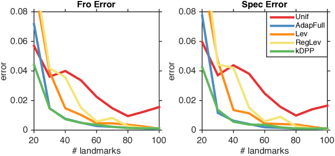
Figure 1: Relative Frobenius/spectral norm errors from different kernel approximations (Ailerons data).

We first explore Dpp-Nyström (kDPP in the figures) for approximating kernel matrices. We compare to uniform sampling (Unif) and leverage score sampling (Lev) [19] as baseline landmark selection methods. We also include AdapFull (AdapFull) [13] that performs quite well in practice but scales poorly, as $\mathcal{O}(N^{2})$, with the size of dataset. Although sampling with regularized leverage scores (RegLev) [2] is not originally designed for kernel approximations, we include its results to see how regularization affects leverage score sampling.

Figure 1 shows example results on the Ailerons data; further results may be found in the appendix. Dpp-Nyström performs well, achieving the lowest error as measured in both spectral and Frobenius norm. The only method that is on par in terms of accuracy is AdapFull, which has a much higher running time.

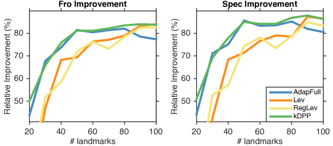
Figure 2: Improvement in relative Frobenius/spectral norm errors (%) over Unif (with corresponding landmark sizes) for kernel approximation, averaged over all datasets.

For a different perspective, Figure 2 shows the improvement in error over Unif. Relative improvements are averaged over all data sets. Again, the performance of Dpp-Nyström almost always dominate those of other methods, and achieves an up to 80% reduction in error.

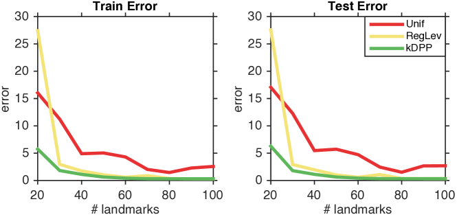
Figure 3: Training and test errors for kernel ridge regression with different Nyström approximations (Ailerons data).

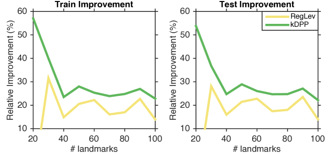
Figure 4: Improvements in training/test errors (%) over uniform sampling (with same number of landmarks) in kernel ridge regression, averaged over all datasets.

6.2 Kernel Ridge Regression

Next, we apply Dpp-Nyström to kernel ridge regression, comparing against uniform sampling (Unif) [5] and regularized leverage score sampling (RegLev) [2] which have theoretical guarantees for this task. Figure 3 illustrates an example result: non-uniform sampling greatly improves accuracy, with kDPP improving over regularized leverage scores in particular for a small number of landmarks, where a single column has a larger effect.

Figure 4 displays the average improvement over Unif, averaged over 8 data sets. Again, the performance of kDPP dominates RegLev and Unif, and leads to gains in accuracy. On average kDPP consistently achieves more than $20\%$ improvement over Unif.

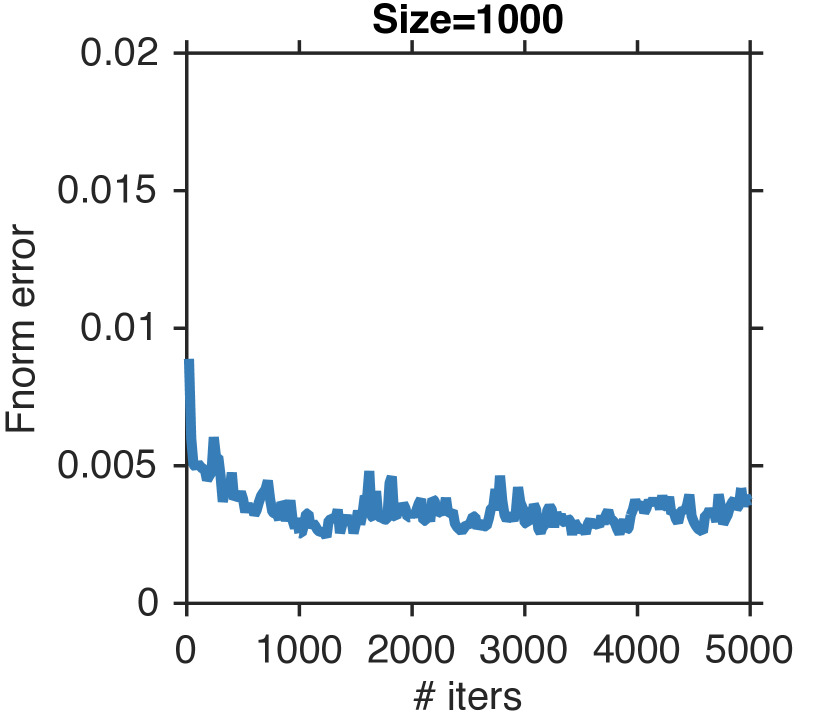
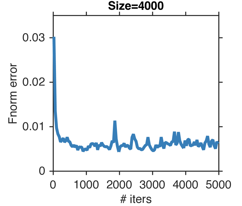
Figure 5: Relative Frobenius norm error of Dpp-Nyström with 50 landmarks as changing across iterations of the Markov Chain (Ailerons data).

6.3 Mixing of the Gibbs Markov Chain

In the next experiment, we empirically study the mixing of the Gibbs chain with respect to matrix approximation errors, the ultimate measure that is of interest in our application of the sampler. We use $c=50$ and choose $N$ as 1,000 and 4,000. To exclude impacts of the initialization, we pick the initial state $Y_{0}$ uniformly at random. We run the chain for 5,000 iterations, monitoring how the error changes with the number of iterations. Example results on the Ailerons data are shown in Figure 5. Empirically, the error drops very quickly and afterwards fluctuates only little, indicating a fast convergence of the approximation error. Other error measures and larger $c$, included in the appendix, confirm this trend.

Notably, our empirical results suggest that the mixing time does not increase much as $N$ increases greatly, suggesting that the Gibbs sampler remains fast even for large $N$.

In Theorem 5, the mixing time depends on the quantity $\alpha$. By subsampling 1,000 random sets $S$ and column indices $r,t$, we approximately computed $\alpha$ on our data sets. We find that, as expected, $\alpha<1$ in particular for kernels with a smaller bandwidth, and in general $\alpha$ increases with $k$. In accordance with the theory, we found that the mixing time (in terms of error) too increases with $k$. In practice, we observe a fast drop in error even for cases where $\alpha>1$, indicating that Theorem 5 is conservative and that the iterative MCMC approach is even more widely applicable.

6.4 Time-Error Tradeoffs

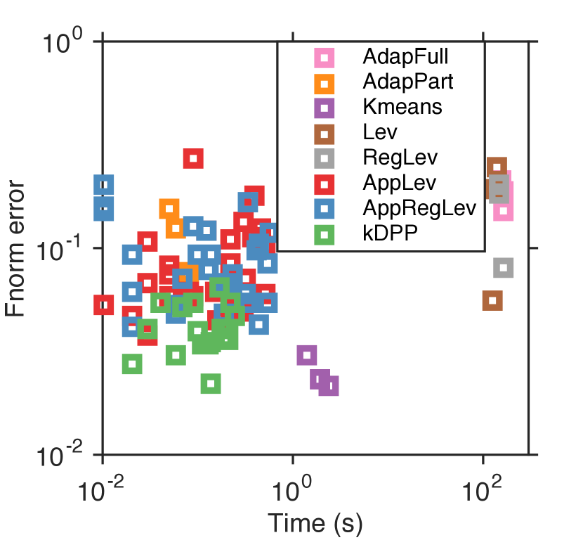
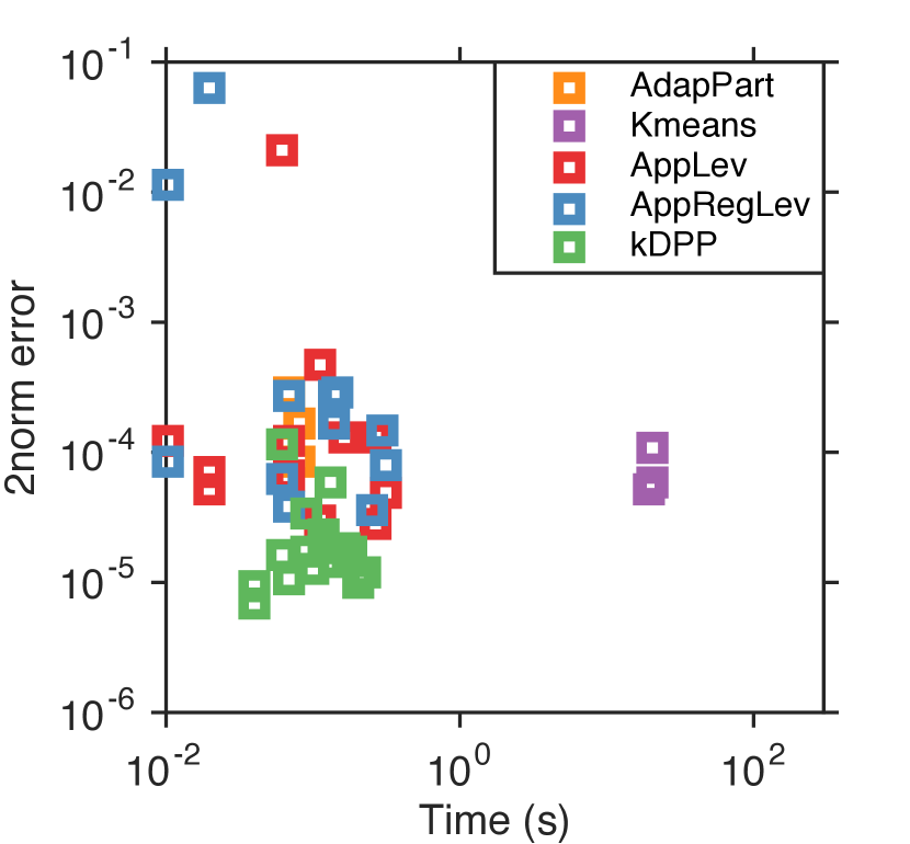
Figure 6: Time-Error tradeoffs with 20 landmarks on Ailerons (size 4,000) and California Housing (size 12,000). Time and Errors are shown on a log scale. Bottom left is the best (low error, low running time), top right is the worst. We did not include AdapFull, Lev and RegLev on California Housing due to their long running times.

Iterative methods like the Gibbs sampler offer tradeoffs between time and error. The longer the Markov Chain runs, the closer the sampling distribution is to the desired Dpp, and the higher the accuracy obtained by Nyström. We hence explicitly show the time and accuracy trade-off of the sampler on Ailerons (of size 4,000) for up to 200 and California Housing (of size 12,000) for up to 100 iterations.

A similar tradeoff occurs with leverage scores. For the experiments in the other sections, we computed the (regularized) leverage scores for Lev and RegLev exactly. This requires a full, computationally expensive eigendecomposition. For a fast, rougher approximation, we here compare to an approximation mentioned in [2]. Concretely, we sample $p$ elements with probability proportional to the diagonal entries of kernel matrices $K_{ii}$, and then use a Nyström-like method to construct an approximate low-rank decomposition of $K$, and compute scores based on this approximation. We vary $p$ from 20 to 340 on Ailerons and 20 to 140 on California Housing to show the tradeoff for approximate leverage score sampling (AppLev) and regularized leverage score sampling (AppRegLev). We also include AdapPartial (AdapPart) [28] that approximates AdapFull and is much more efficient, and Kmeans Nyström (Kmeans) [44] that empirically perform very well in kernel approximation.

Figure 6 summarizes and compares the tradeoffs offered by these different methods on the Ailerons and California Housing datasets. The $x$ axis indicates time, the $y$ axis error, so the lower left is the preferred corner. We see that AdapFull, Lev and RegLev are expensive and perform worse than kDPP. The approximate variants AdapPart, AppLev and AppRegLev have comparable efficiency but higher error. On the smaller data, Kmeans is accurate but needs more time than kDPP, while on the larger data it is dominated in both accuracy and time by kDPP. Overall, on the larger data, Dpp-Nyström offers the best tradeoff of accuracy and efficiency.

7 Conclusion

In this paper, we revisited the use of $k$-Determinantal Point Processes for sampling good landmarks for the Nyström method. We theoretically and empirically observe its competitive performance, for both matrix approximation and ridge regression, compared to state-of-the-art methods.

To make this accurate method scalable to large matrices, we consider an iterative approach, and analyze it theoretically as well as empirically. Our results indicate that the iterative approach, a Gibbs sampler, achieves good landmark samples quickly; under certain conditions even in a number of iteratons linear in $N$, for an $N$ by $N$ matrix. Finally, our empirical results demonstrate that among state-of-the-art methods, the iterative sampler yields the best tradeoff between efficiency and accuracy.

Acknowledgements

This research was partially supported by an NSF CAREER award 1553284, NSF grant IIS-1409802, and a Google Research Award. We also thank Xixian Chen for discussions.

Appendix A Bounds that hold with High Probability

To show high probability bounds we employ concentration results on homogeneous strongly Rayleigh measures. Specifically, we use the following theorem.

Theorem 6 (Pemantle and Peres [33]).

Let $\mathbb{P}$ be a $k$-homogeneous strongly Rayleigh probability measure on $\{0,1\}^{N}$ and $f$ an $\ell$-Lipschitz function on $\{0,1\}^{N}$, then

$$\mathbb{P}(f-\mathbb{E}[f]\geq a\ell)\leq\exp\{-a^{2}/8k\}.$$

It is known that a $k$-Dpp is a homogeneous strongly Rayleigh measure on $\{0,1\}^{N}$ [10, 4], thus Theorem 6 applies to results obtained with $k$-Dpp. Concretely, for the bound in Theorem 1 that holds in expectation, we have the following bound that holds with high probability:

Corollary 7.

When sampling $C\sim k$-Dpp($K$), for any $\delta\in(0,1)$, with probability at least $1-\delta$ we have

$${\|K-K_{\cdot C}(K_{C,C})^{\dagger}K_{C\cdot}\|_{F}\over\|K-K_{k}\|_{F}}\leq\left(\frac{c+1}{c+1-k}\right)\sqrt{N-k}+\sqrt{8c\log(1/\delta)}\sqrt{\sum_{i=1}^{N}\lambda_{i}^{2}\over\sum_{i=k+1}^{N}\lambda_{i}^{2}},$$

$${\|K-K_{\cdot C}(K_{C,C})^{\dagger}K_{C\cdot}\|_{2}\over\|K-K_{k}\|_{2}}\leq\left({c+1\over c+1-k}\right)(N-k)+\sqrt{8c\log(1/\delta)}\tfrac{\lambda_{1}}{\lambda_{k+1}},$$

where $\lambda_{1}\geq\lambda_{2}\geq\ldots\geq\lambda_{N}$ are the eigenvalues of $K$.

Proof.

The Lipschitz constants of the relative errors are upper bounded by $\sqrt{\sum_{i=1}^{N}\lambda_{i}^{2}\over\sum_{i=k+1}^{N}\lambda_{i}^{2}}$ and ${\lambda_{1}\over\lambda_{k+1}}$, respectively. Applying Theorem 6 yields the results.

∎

For the bound in Theorem 3 that holds in expectation, we have the following bound that holds with high probability:

Corollary 8.

If $\tilde{K}$ is constructed via Dpp-Nyström, then with probability at least $1-\delta$, $\sqrt{\mathrm{bias}(\tilde{K})\over\mathrm{bias}(K)}$ is upper-bounded by

$$1+{1\over N\gamma}\left({(c+1)e_{c+1}(K)\over e_{c}(K)}+\sqrt{8c\log(1/\delta)}\text{tr}(K)\right).$$

Proof.

Consider the function $f_{C}(K)=\nu_{C}=\sum_{i}\|b_{i}^{\top}(U^{C})^{\perp}\|_{2}^{2}\leq\sum_{i}\|b_{i}^{\top}\|_{2}^{2}=\text{tr}(K)$. Since $0\leq f_{C}(K)\leq\text{tr}(K)$, it follows that the Lipschitz constant for $f_{C}$ is at most $\text{tr}(K)$. Thus when $C\sim k$-Dpp and $\delta\in(0,1)$, by applying Theorem 6 we see that the inequality $\nu_{C}\leq\mathbb{E}\left[\nu_{C}\right]+\sqrt{8c\log(1/\delta)}\text{tr}(K)$ holds with probability at least $1-\delta$. Hence

$$\mathbb{E}_{C}\left[\sqrt{\mathrm{bias}(\tilde{K})\over\mathrm{bias}(K)}\right]\leq 1+\mathbb{E}\left[{\nu_{C}\over N\gamma}\right]+\sqrt{8c\log(1/\delta)}{\text{tr}(K)\over N\gamma}$$

$$\;\;\;\;=1+{1\over N\gamma}\left({(c+1)e_{c+1}(K)\over e_{c}(K)}+\sqrt{8c\log(1/\delta)}\text{tr}(K)\right)$$

holds with probability at least $1-\delta$. ∎

Appendix B Supplementary Experiments

B.1 Kernel Approximation

Fig. 7 shows the matrix norm relative error of various methods in kernel approximation on the remaining 7 datasets mentioned in the main text.

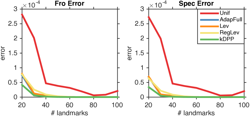
(a) Abalone

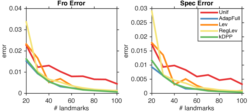
(b) Bank8FM

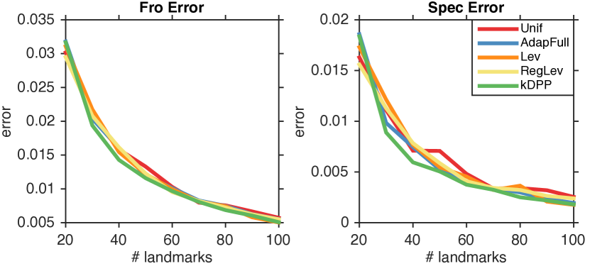
(c) Bank32NH

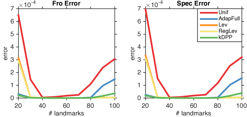
(d) California Housing

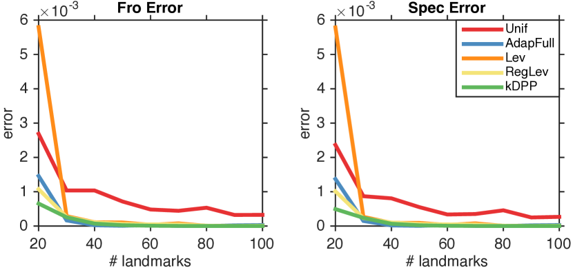
(e) CompAct

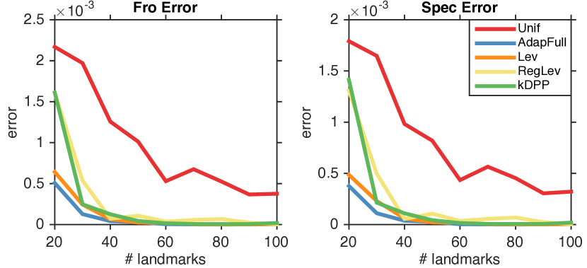
(f) CompAct(s)

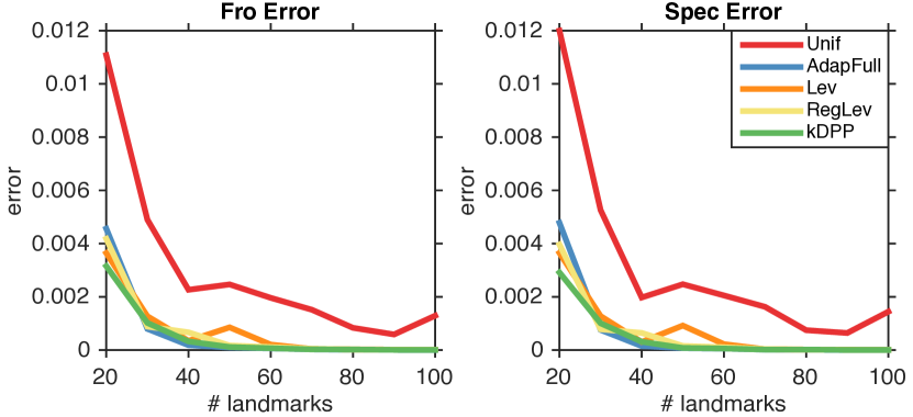
(g) Elevators

Figure 7: Relative Frobenius norm and spectral norm error achieved by different kernel approximation algorithms on the remaining 7 data sets.

B.2 Approximated Kernel Ridge Regression

Fig. 8 shows the training and test error of various methods for kernel ridge regression on the remaining 7 datasets.

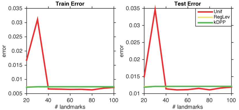
(a) Abalone

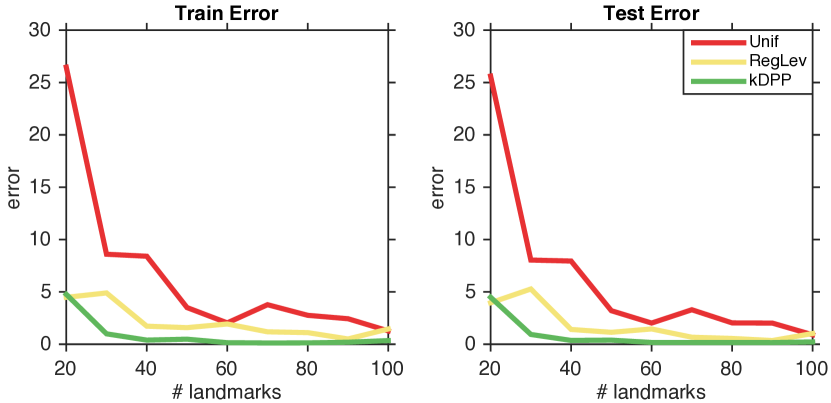
(b) Bank8FM

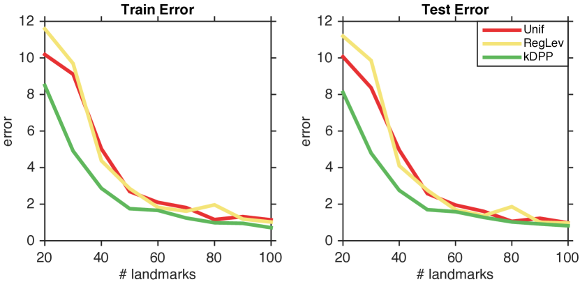
(c) Bank32NH

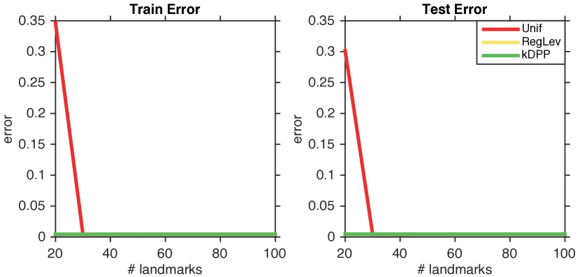
(d) California Housing

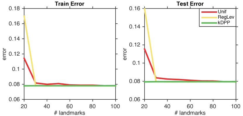
(e) CompAct

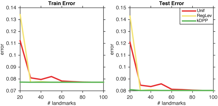
(f) CompAct(s)

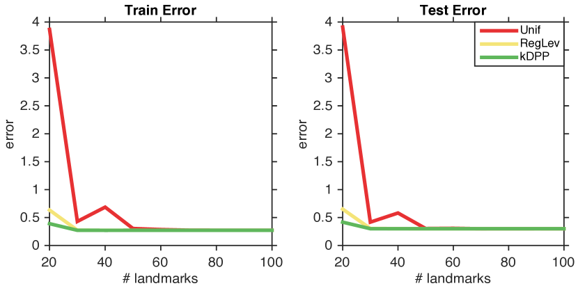
(g) Elevators

Figure 8: Training and test error achieved by different Nyström kernel ridge regression algorithms on the remaining 7 regression datasets.

B.3 Mixing of Markov Chain $k$-Dpp

We first show the mixing of the Gibbs Dpp-Nyström with 50 landmarks with different performance measures: relative spectral norm error, training error and test error of kernel ridge regression in Fig. 9.

We also show corresponding results with respect to 100 and 200 landmarks in Fig. 10 and Fig. 11, so as to illustrate that for varying number of landmarks the chain is indeed fast mixing and will give reasonably good result within a small number of iterations.

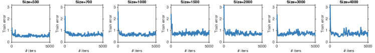
(a) Training error

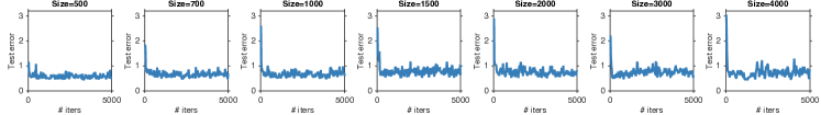
(b) Test error

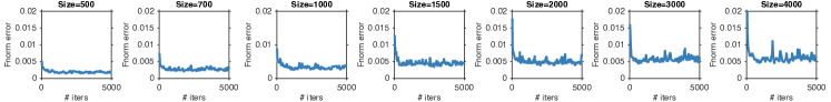
(c) Relative Frobenius norm error

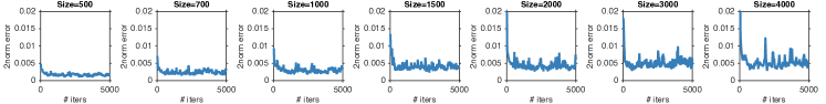
(d) Relative Spectral norm error

Figure 9: Performance of Markov chain Dpp-Nyström with 50 landmarks on Ailerons. Runs for 5,000 iterations.

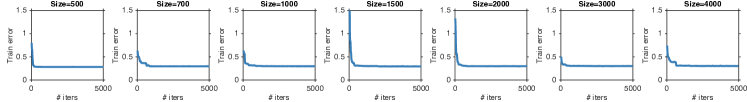
(a) Training error

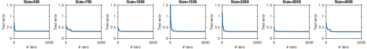
(b) Test error

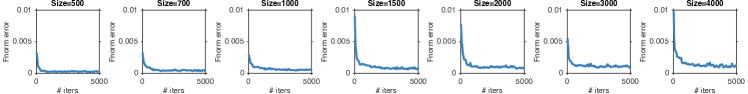
(c) Relative Frobenius norm error

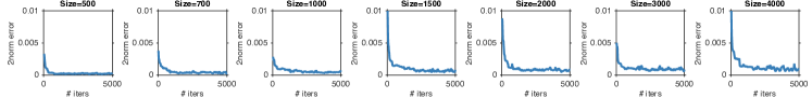
(d) Relative Spectral norm error

Figure 10: Performance of Markov chain Dpp-Nyström with 100 landmarks on Ailerons. Runs for 5,000 iterations.

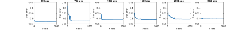
(a) Training error

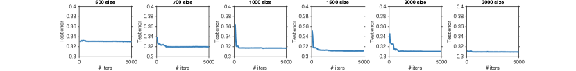
(b) Test error

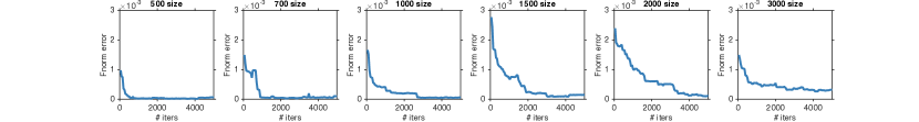
(c) Relative Frobenius norm error

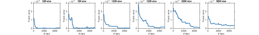
(d) Relative Spectral norm error

Figure 11: Performance of Markov chain Dpp-Nyström with 200 landmarks on Ailerons. Runs for 5,000 iterations.

B.4 Running Time Analysis

We next show time-error trade-offs for various sampling methods on small and larger datasets with respect to Fnorm and 2norm errors. We sample 20 landmarks from Ailerons dataset of size 4,000 and California Housing of size 12,000. The result is shown in Figure 12 and Figure 13 and similar trends as the example results in the main text could be spotted: on small scale dataset (size 4,000) kDPP get very good time-error trade-off. It is more efficient than Kmeans, though the error is a bit larger. While on larger dataset (size 12,000) the efficiency is further enhanced while the error is even lower than Kmeans. It also have lower variances in both cases compared to AppLev and AppRegLev. Overall, on larger dataset we obtain the best time-error trade-off with kDPP.

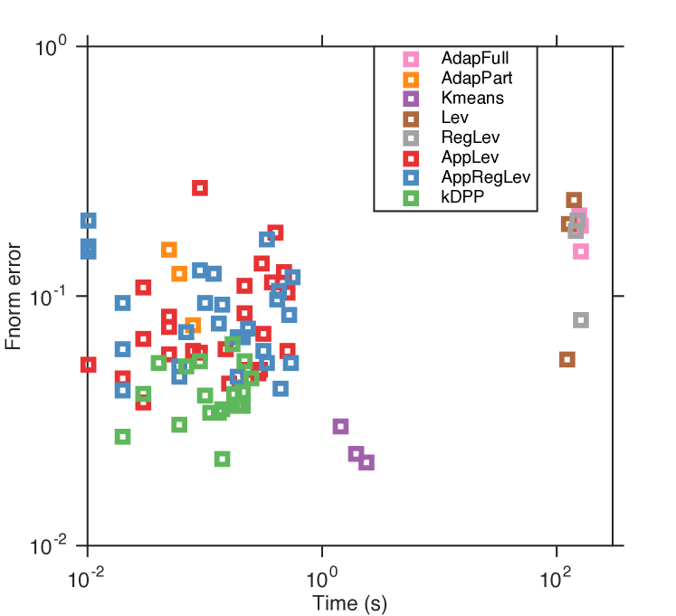
(a) Fnorm Error vs. Time

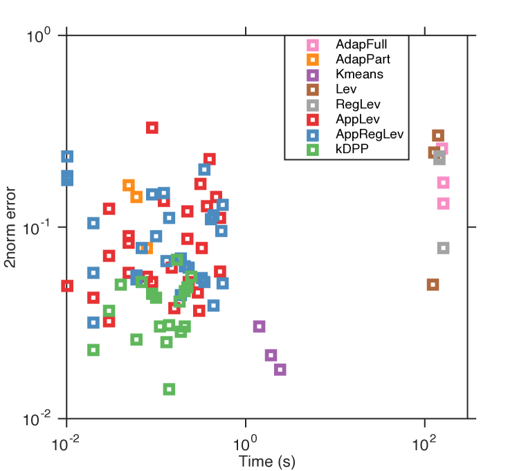
(b) 2norm Error vs. Time

Figure 12: Time-Error tradeoff with 20 landmarks on Ailerons of size 4,000. Time and Errors shown in log-scale.

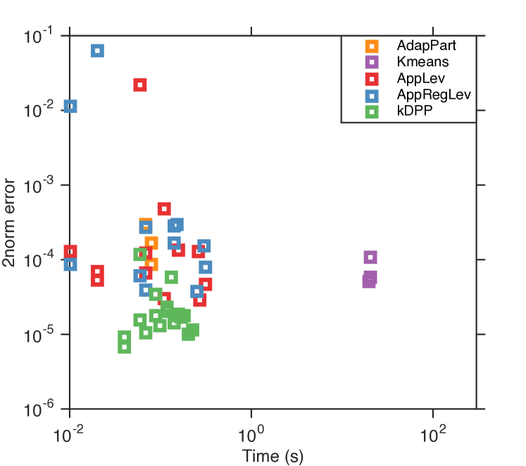
(a) 2norm Error vs. Time

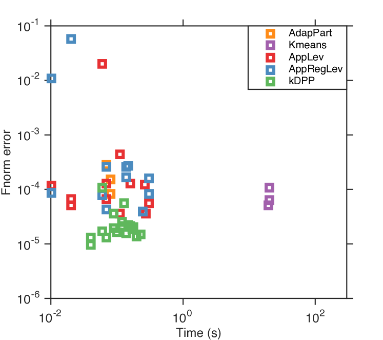
(b) Training Error vs. Time

Figure 13: Time-Error tradeoff with 20 landmarks on California Housing of size 12,000. Time and Errors shown in log-scale. We didn’t include AdapFull, Lev and RegLev due to their inefficiency on larger datasets.

References

- Affandi et al. [2013] R. H. Affandi, A. Kulesza, E. Fox, and B. Taskar. Nyström approximation for large-scale determinantal processes. In AISTATS, pages 85–98, 2013.
- Alaoui and Mahoney [2015] A. E. Alaoui and M. W. Mahoney. Fast randomized kernel methods with statistical guarantees. NIPS, 2015.
- Aldous [1982] D. J. Aldous. Some inequalities for reversible Markov chains. Journal of the London Mathematical Society, pages 564–576, 1982.
- Anari et al. [2016] N. Anari, S. O. Gharan, and A. Rezaei. Monte Carlo Markov chain algorithms for sampling strongly Rayleigh distributions and determinantal point processes. In COLT, 2016.
- Bach [2013] F. R. Bach. Sharp analysis of low-rank kernel matrix approximations. COLT, 2013.
- Bach and Jordan [2003] F. R. Bach and M. I. Jordan. Kernel independent component analysis. JMLR, pages 1–48, 2003.
- Bach and Jordan [2005] F. R. Bach and M. I. Jordan. Predictive low-rank decomposition for kernel methods. In ICML, pages 33–40, 2005.
- Belabbas and Wolfe [2009a] M.-A. Belabbas and P. J. Wolfe. On landmark selection and sampling in high-dimensional data analysis. Philosophical Transactions of the Royal Society of London A: Mathematical, Physical and Engineering Sciences, pages 4295–4312, 2009a.
- Belabbas and Wolfe [2009b] M.-A. Belabbas and P. J. Wolfe. Spectral methods in machine learning and new strategies for very large datasets. Proceedings of the National Academy of Sciences, pages 369–374, 2009b.
- Borcea et al. [2009] J. Borcea, P. Brändén, and T. Liggett. Negative dependence and the geometry of polynomials. Journal of the American Mathematical Society, pages 521–567, 2009.
- Bubley and Dyer [1997] R. Bubley and M. Dyer. Path coupling: A technique for proving rapid mixing in Markov chains. In FOCS, pages 223–231, 1997.
- Cortes et al. [2010] C. Cortes, M. Mohri, and A. Talwalkar. On the impact of kernel approximation on learning accuracy. In AISTATS, pages 113–120, 2010.
- Deshpande et al. [2006] A. Deshpande, L. Rademacher, S. Vempala, and G. Wang. Matrix approximation and projective clustering via volume sampling. In SODA, pages 1117–1126, 2006.
- Drineas and Mahoney [2005] P. Drineas and M. W. Mahoney. On the Nyström method for approximating a Gram matrix for improved kernel-based learning. JMLR, pages 2153–2175, 2005.
- Drineas et al. [2006] P. Drineas, R. Kannan, and M. W. Mahoney. Fast Monte Carlo algorithms for matrices II: Computing a low-rank approximation to a matrix. SIAM Journal on Computing, pages 158–183, 2006.
- Dyer and Greenhill [1998] M. Dyer and C. Greenhill. A more rapidly mixing Markov chain for graph colorings. Random Structures and Algorithms, pages 285–317, 1998.
- Fine and Scheinberg [2002] S. Fine and K. Scheinberg. Efficient SVM training using low-rank kernel representations. JMLR, pages 243–264, 2002.
- Fowlkes et al. [2004] C. Fowlkes, S. Belongie, F. Chung, and J. Malik. Spectral grouping using the Nyström method. TPAMI, pages 214–225, 2004.
- Gittens and Mahoney [2013] A. Gittens and M. W. Mahoney. Revisiting the Nyström method for improved large-scale machine learning. ICML, 2013.
- Golub and Van Loan [2012] G. H. Golub and C. F. Van Loan. Matrix computations. JHU Press, 2012.
- Gotovos et al. [2015] A. Gotovos, H. Hassani, and A. Krause. Sampling from probabilistic submodular models. In NIPS, pages 1936–1944, 2015.
- Guruswami and Sinop [2012] V. Guruswami and A. K. Sinop. Optimal column-based low-rank matrix reconstruction. In SODA, pages 1207–1214, 2012.
- Hough et al. [2006] J. B. Hough, M. Krishnapur, Y. Peres, and B. Virág. Determinantal processes and independence. Probability Surveys, pages 206–229, 2006.
- Kang [2013] B. Kang. Fast determinantal point process sampling with application to clustering. In NIPS, pages 2319–2327, 2013.
- Kulesza and Taskar [2011] A. Kulesza and B. Taskar. k-DPPs: Fixed-size determinantal point processes. In ICML, pages 1193–1200, 2011.
- Kulesza and Taskar [2012] A. Kulesza and B. Taskar. Determinantal point processes for machine learning. arXiv preprint arXiv:1207.6083, 2012.
- Kumar et al. [2009] S. Kumar, M. Mohri, and A. Talwalkar. Ensemble Nyström method. In NIPS, pages 1060–1068, 2009.
- Kumar et al. [2012] S. Kumar, M. Mohri, and A. Talwalkar. Sampling methods for the nyström method. The Journal of Machine Learning Research, pages 981–1006, 2012.
- Li et al. [2016a] C. Li, S. Jegelka, and S. Sra. Efficient sampling for k-determinantal point processes. AISTATS, 2016a.
- Li et al. [2016b] C. Li, S. Sra, and S. Jegelka. Gaussian quadrature for matrix inverse forms with applications. In ICML, 2016b.
- Macchi [1975] O. Macchi. The coincidence approach to stochastic point processes. Advances in Applied Probability, pages 83–122, 1975.
- Nyström [1930] E. J. Nyström. Über die praktische Auflösung von Integralgleichungen mit Anwendungen auf Randwertaufgaben. Acta Mathematica, pages 185–204, 1930.
- Pemantle and Peres [2014] R. Pemantle and Y. Peres. Concentration of Lipschitz functionals of determinantal and other strong Rayleigh measures. Combinatorics, Probability and Computing, pages 140–160, 2014.
- Rebeschini and Karbasi [2015] P. Rebeschini and A. Karbasi. Fast mixing for discrete point processes. COLT, 2015.
- Rudi et al. [2015] A. Rudi, R. Camoriano, and L. Rosasco. Less is more: Nyström computational regularization. NIPS, 2015.
- Shen et al. [2009] H. Shen, S. Jegelka, and A. Gretton. Fast kernel-based independent component analysis. IEEE Transactions on Signal Processing, pages 3498–3511, 2009.
- Smola and Schölkopf [2000] A. J. Smola and B. Schölkopf. Sparse greedy matrix approximation for machine learning. ICML, 2000.
- Sun et al. [2015] S. Sun, J. Zhao, and J. Zhu. A review of Nyström methods for large-scale machine learning. Information Fusion, pages 36–48, 2015.
- Talwalkar et al. [2008] A. Talwalkar, S. Kumar, and H. Rowley. Large-scale manifold learning. In CVPR, 2008.
- Talwalkar et al. [2013] A. Talwalkar, S. Kumar, M. Mohri, and H. Rowley. Large-scale SVD and manifold learning. JMLR, pages 3129–3152, 2013.
- Vondrák [2013] J. Vondrák. Symmetry and approximability of submodular maximization problems. SIAM Journal on Computing, 42(1):265–304, 2013.
- Wang et al. [2014] S. Wang, C. Zhang, H. Qian, and Z. Zhang. Using the matrix ridge approximation to speedup determinantal point processes sampling algorithms. In AAAI, 2014.
- Williams and Seeger [2001] C. Williams and M. Seeger. Using the Nyström method to speed up kernel machines. In NIPS, pages 682–688, 2001.
- Zhang et al. [2008] K. Zhang, I. W. Tsang, and J. T. Kwok. Improved Nyström low-rank approximation and error analysis. In ICML, pages 1232–1239, 2008.