Non-standard conditionally specified models for non-ignorable missing data

Abstract

Data analyses typically rely upon assumptions about missingness mechanisms that lead to observed versus missing data. When the data are missing not at random, direct assumptions about the missingness mechanism, and indirect assumptions about the distributions of observed and missing data, are typically untestable. We explore an approach, where the joint distribution of observed data and missing data is specified through non-standard conditional distributions. In this formulation, which traces back to a factorization of the joint distribution, apparently proposed by J.W. Tukey, the modeling assumptions about the conditional factors are either testable or are designed to allow the incorporation of substantive knowledge about the problem at hand, thereby offering a possibly realistic portrayal of the data, both missing and observed. We apply Tukey’s conditional representation to exponential family models, and we propose a computationally tractable inferential strategy for this class of models. We illustrate the utility of this approach using high-throughput biological data with missing data that are not missing at random.

Keywords: Missing data; missing not at random; non-ignorable missing data mechanisms; Tukey’s representation; conditionally specified models; Bayesian analysis.

1 Introduction

Missing data are ubiquitous in applications of statistics, including survey sampling, healthcare, public policy and bioinformatics. The effort needed for modeling and analyzing observations in these situations crucially depends on the mechanism that induces the missing data as well as on the mode of inference (Little and Rubin, 2014).

Here, we work within the inferential framework outlined in Rubin (2004). The inferential target of interest is generally a function of observed and missing data. One key concept is that of a “missing at random” missing data mechanism, for which the conditional probability distribution of the missingness indicators is a function only of the observed data, and the related concept of ignorable missing data (Rubin, 1976, 1978; Mealli and Rubin, 2015). For Bayesian inference, ignorability implies that the posterior distribution of the target is conditionally independent of the observation indicators, given the observed data, and so there is no need to specify a model for observation indicators to achieve valid Bayesian or likelihood-based inference. When the posterior distribution of the inferential target depends on these indicators, valid Bayesian inference requires specifying a joint model for the data and the indicators.

With missing data, there are two basic approaches to specify the the joint distribution of the complete data and missing data indicators given parameters, and the implied likelihood, as a product of marginal and conditional distributions. The first basic approach (Rubin, 1974) is to posit a standard model for the complete data, and then specify an explicit model that selects observed data from the complete data, called the missingness mechanism (Rubin, 1976). The second basic approach is to specify separate distributions for the observed data and the missing data, thus eschewing explicit assumptions about the missingness mechanism (Rubin, 1977; Little, 1993). The fundamental challenge with these two basic approaches is that some assumptions about the missingness mechanism, whether explicit or implicit, are typically not testable from the observed data. As a result, some literature on inference in the presence of missing data centers on assessing sensitivity to different model specifications (Rubin, 1977; Scharfstein et al., 1999; Andrea et al., 2001; Little and Rubin, 2014).

1.1 Contributions

Here, we develop an alternative approach to modeling data possibly missing not at random, evidentially originally proposed by Tukey and discussed by Hartigan and Rubin, reported by Holland (1986). The key insight is to represent the joint distribution of the complete data and missing-data indicators as proportional to factors that involve only observed values and the missingness mechanism. Assumptions about these factors are either testable, or typically allow the incorporation of substantive knowledge about the problem at hand, thereby offering a clear path to eliciting a realistic portrayal of the sources of variation in the data.

In Section 2, we review the two basic model specifications for missing data, before formally introducing Tukey’s representation. In Section 3, we discuss technical issues involved when using Tukey’s representation, and provide a full characterization for exponential-family models. In Section 4, we then illustrate the use of these models on simulated data when the model is correctly specified, when the model is incorrectly specified, and on an application in biology. In Section 5, we offer theoretical insights and use them to state formal results.

2 Basic models for missing data

Discussion of models using basic factorizations for missing data can be found in a variety of places, including Glynn et al. (1986) and Molenberghs et al. (2015).

Throughout, let $Y=(Y_{1},Y_{2},...,Y_{N})^{\intercal}$ represent the complete data and $R=(R_{1},R_{2},...,R_{N})^{\intercal}$ represent the response indicators for $Y$, which are “missing” when $R_{i}$=0 and “observed” when $R_{i}=1$. The joint distribution, assuming $(Y_{i},R_{i})$ are i.i.d., is then

$$P(Y,R\mid\theta)=\prod_{i}f(Y_{i},R_{i}\mid\theta),$$

where $\theta$ is a parameter vector. For simplicity, we focus on the the case without covariates.

2.1 The selection factorization

The selection approach (Rubin, 1974) factors the joint distribution of $(Y,R)$ as

$$P(Y,R\mid\theta)=\prod_{i}^{N}f(Y_{i}|\theta_{Y})f(R_{i}|Y_{i},\theta_{R|Y}),$$ (1)

using the distribution of the complete data, $P(Y|\theta_{Y})$, and the missingness mechanism, or selection function, $P(R|Y,\theta_{R|Y})$, which controls which data are actually observed, where the parameters $(\theta_{Y},\theta_{R|Y})$, are functions of $\theta$. Models for $f(Y_{i}|\theta_{Y})$ include the normal, with $\theta_{Y}$ the mean and variance of the normal, or the Bernoulli with $\theta_{Y}$ the probability of success of the Bernoulli. Typical models for $f(R_{i}|Y_{i},\theta_{R|Y})$ include the logistic and probit models (e.g., see Gelman et al., 2004).

2.2 The pattern-mixture factorization

The pattern-mixture approach (Rubin, 1977; Little, 1993; Little and Rubin, 2014) is the alternative basic factorization; the complete data distribution is specified as a mixture of observed and missing data components,

$$P(Y,R|\theta) = \prod_{i=1}^{N}f(Y_{i}|R_{i},\theta_{Y|R})f(R_{i}|\theta_{R})$$ (2)

$$= \prod_{i=1}^{N}\prod_{r=0}^{1}\left[f(Y_{i}|R_{i}=r,\theta_{Y|R=r})f(R_{i}=r|\theta_{R})\right]^{I(R_{i}=r)},$$

where $(\theta_{Y|R},\theta_{R})$ are functions of $\theta$, leading to a mixture likelihood, which for a single observation is

$$P(Y_{i}\mid\theta)=\sum_{r=0}^{1}f(Y_{i}|R_{i}=r,\theta_{Y|R=r})f(R_{i}=r|\theta_{R}).$$

The model for $f(R_{i}|\theta_{R})$ is a Bernoulli distribution with parameter $\theta_{R}$. The model for $f(Y_{i}|R_{i}=1)$ is typically chosen to fit the observed data well, whereas the model for $f(Y_{i}|R_{i}=0)$ is commonly chosen to be a location shift or scale change of $f(Y_{i}|R_{i}=1)$ (e.g., see Gelman et al., 2004; Little and Rubin, 2014).

2.3 Tukey’s representation

John W. Tukey, in a discussion of Glynn et al. (1986), suggested an alternative factorization of the joint distribution for $(Y,R)$ in terms of conditional distributions (recorded in Holland, 1986), which he refers to as the simplified selection model, with parameters $\theta_{Y|R=1}$ and $\theta_{R|Y}$,

$$P(Y,R\mid\theta)\propto\prod_{i=1}^{N}f(Y_{i}\mid R_{i}=1,\theta_{Y|R=1})\cdot\frac{f(R_{i}\mid Y_{i},\theta_{R|Y})}{f(R_{i}=1\mid Y_{i},\theta_{R|Y})},$$ (3)

with normalizing constant $\prod_{i=1}^{N}f(R_{i}=1\mid\theta_{R|Y},\theta_{Y|R=1})$ ensuring integrability. As Holland notes, a main advantage of this factorization is that it only involves the observed data density, $f(Y_{i}\mid R_{i}=1,\theta_{Y|R=1})$, which can be estimated directly, and the missingness mechanism, $f(R_{i}\mid Y_{i},\theta_{R|Y})$, which can be easy to elicit in the context of a specific application.

Tukey’s representation can be obtained through a simple application of Brook’s lemma, which equates the ratio of joint distributions to the ratio of their full conditionals (Brook, 1964; Besag, 1974). Although this lemma is most commonly referenced in the theory of spatial autoregressive models (Cressie, 2011), its connection to Tukey’s representation is relevant because it immediately reveals some theoretical insights. Importantly, Brook’s Lemma is only applicable when the so-called positivity condition is satisfied (Hammersley and Clifford, 1971), which for Tukey’s representation means that

$$\text{If: }P(R_{i}=r|\theta)>0\text{ and }P(Y_{i}=y|\theta)>0$$

$$\text{Then: }P(R_{i}=r,Y_{i}=y|\theta)>0$$

for all pairs of values $(r,y)$. This condition is not trivially satisfied in missing data problems. For instance, Tukey’s representation cannot be applied to models where $P(R_{i}=1|Y_{i}<c,\theta_{R|Y})=0$, deterministically, for some cutoff $c$, as when the complete data model is normal and the observed data model is truncated normal. Consequently, here we focus on problems where $P(R_{i}=1|Y_{i},\theta_{R|Y})>0$, that is, where the support of the missing data is contained in the support of the observed data.

In addition, the conditional distributions specified in Equation 3 must imply an integrable joint density (Besag, 1974). With Tukey’s representation, the integrability condition constrains the rate at which the tails of the distribution for observed data decrease relative to the rate at which the odds of a missing value increase. This condition is illustrated in Section 4.1, and discussed in Section 5.2.

3 Modeling and inference using Tukey’s representation

Let $P(Y_{i}=y_{i}\mid R_{i}=1,\theta_{Y_{i}|R_{i}=1})$ be denoted $f^{\rm obs}(y_{i}\mid\theta_{Y|R})$, for simplicity. Using Equation 3, we can write the density for $(y_{i},r_{i})$ as

$$f(y_{i},r_{i}\mid\theta_{R|Y},\theta_{Y|R}) \propto \begin{cases}f^{\rm obs}(y_{i}\mid\theta_{Y|R})&\mbox{if }r_{i}=1\\ \frac{f(r_{i}=0\mid y_{i},\theta_{R|Y})}{f(r_{i}=1\mid y_{i},\theta_{R|Y})}f^{\rm obs}(y_{i}\mid\theta_{Y|R})&\mbox{if }r_{i}=0\\ \end{cases}$$ (4)

$$= f(r_{i}=1\mid y_{i},\theta_{R|Y})^{r_{i}-1}f(r_{i}=0\mid y_{i},\theta_{R|Y})^{1-r_{i}}f^{\rm obs}(y_{i}\mid\theta_{Y|R})$$

with normalizing constant

$$Q(\theta_{Y|R},\theta_{R|Y}) = \left(1+\int\frac{f(r_{i}=0\mid y_{i},\theta_{R|Y})}{f(r_{i}=1\mid y_{i},\theta_{R|Y})}f^{\rm obs}(y_{i}\mid\theta_{Y|R})~{}dy_{i}\right)^{-1},$$ (5)

which ensures the integral of Equation 4 over random variables $R$ and $Y$ times $Q$ is unity.

The normalizing constant $Q$ is generally difficult to compute. As a consequence, the missing data density cannot easily be expressed. Below, we introduce a class of models for which computation of the normalizing constant is tractable and which also implies simple distributional forms for the missing data and complete data densities.

3.1 Exponential family models

Assume that the observed data distribution belongs to an exponential family and that the logit of the missingness mechanism is linear in the sufficient statistics of that family, which is related to the exponential tilt pattern-mixture models introduced by Birmingham et al. (2003). Formally, let $f^{\rm obs}(y_{i}\mid\theta_{Y|R=1})$ be an exponential family distribution with natural parameter $\theta_{Y|R=1}$. Then,

$$f^{\rm obs}(y_{i}\mid\theta_{Y|R=1})=h(y_{i})g(\theta_{Y|R=1})e^{T(y_{i})^{\prime}\theta_{Y|R=1}},$$ (6)

where $g(\theta_{Y|R=1})$ is the normalizing constant and $T(y_{i})$ is the natural sufficient statistic, possibly multivariate. The missingness mechanism

$$f(r_{i}=1\mid y_{i},\theta_{R|Y})=\hbox{logit }(T(y_{i})^{\prime}\theta_{R|Y})=\frac{1}{1+e^{-\theta_{R|Y}}}$$ (7)

implies that

$$\frac{f(r_{i}=0\mid y_{i},\theta_{R|Y})}{f(r_{i}=1\mid y_{i},\theta_{R|Y})}=e^{-T(y_{i})\theta_{R|Y}}.$$

Then the normalizing constant $Q$ in Equation 5 can be written as a simple function of the normalizing constant $g(\cdot)$ in the exponential family formulation of $f^{\rm obs}$,

$$Q(\theta_{Y|R=1},\theta_{R|Y}) = \frac{g({\theta_{Y|R=1}}+{\theta_{R|Y}})}{g({\theta_{Y|R=1}}+{\theta_{R|Y}})+g(\theta_{Y|R=1})}.$$ (8)

For the class of exponential-logistic models defined by Equations 6–7, the missing data distribution, as specified in Equation 9, is from the same exponential family as the observed data with natural parameter $\theta_{Y|R=0}=\theta_{Y|R=1}+\theta_{R|Y}$,

$$f^{\rm mis}(y\mid\theta_{Y|R=1},\theta_{R|Y})=h(y)g(\theta_{Y|R=0})e^{{T(y)}^{\prime}\theta_{Y|R=0}}.$$ (9)

Thus, missing data imputation with this class of models is straightforward.

In Tukey’s representation, the main source of uncertainty about any inferential target is due to the missingness mechanism, and the prior distribution on $\theta_{R|Y}$.

3.2 Estimation and inference

The primary estimands of interest are typically functions of the parameters specifying the complete-data distribution, $(\theta_{Y|R=1},\theta_{R|Y})$. Because the observed and missing data densities for exponential-logistic models are exponential families, see Equations 6 and 9, the complete-data distribution is a mixture of exponential families. Further, analytic expressions for the normalizing constant $Q$ and the likelihood are available, and thus standard Markov Chain Monte Carlo methods are applicable (Robert and Casella, 2004).

We take a simple approach to inference via Markov Chain Monte Carlo, which is computationally less demanding than with samplers that explicitly characterize the geometry of the solution space, as discussed in Section 5. Consider a simple Normal-logistic model as an illustration, with $\theta_{R|Y}=(\beta_{0},\beta_{1})=\beta\in R^{2}$ with $\beta_{0}$ corresponding to the intercept and $\beta_{1}$ the rate at which the odds of selection change in $T(y)=y$:

$$f(r_{i}=1\mid y_{i},\beta) = \hbox{logit }(\beta_{0}+\beta_{1}y_{i})=\bigm{(}1+\exp\{-\beta_{0}-\beta_{1}y_{i}\}\bigm{)}^{-1}$$

$$f^{\rm obs}(y_{i}) = \hbox{Normal }(0,1).$$

Rather than specifying a prior distribution on $(\beta_{0},\beta_{1})$, we specify a prior distribution on $Q$ and $\beta_{1}$, but not on $\beta_{0}$. We then invert Equation 8 and solve for $\beta_{0}$ to get,

$$\beta_{0}(Q,\eta,\beta_{1})=\text{log}\left(\frac{g(\eta+\beta_{1})(1-Q)}{g(\eta)}\right).$$ (10)

In this Normal-logistic example, the standard Normal has natural parameters $(\eta_{1},\eta_{2})=(0,-1/2)$, and $g(\eta)=-\frac{\eta_{1}^{2}}{4\eta_{2}}-\frac{1}{2}\ln(-2\eta_{2})$. Thus, Equation 8 becomes,

$$Q(\beta_{0},\beta_{1})=\frac{\beta_{1}^{2}}{\beta_{1}^{2}-2e^{\beta_{0}}},$$

and solving Equation 10 we get

$$\beta_{0}=\text{log}\left(\frac{\beta_{1}^{2}(1-Q)}{2}\right).$$

Next, we use this inferential strategy to demonstrate the utility of Tukey’s representation.

4 Numerical examples and an application in biology

In Section 4.1, we explore selection, pattern-mixture, and Tukey representations for missing data using simulation studies, where $f^{\rm obs}(y_{i}\mid r_{i}=1,\theta_{Y|R=1})$ is a mixture of exponential family distributions. In this example, we discuss how both the selection and the pattern mixture factorizations require difficult modeling choices in practice, and illustrate how Tukey’s representation can be employed with relative ease. In Section 4.2 we explore the robustness of logistic-exponential family missing-data models when the true generating process cannot be expressed as a finite mixture of exponential families. In Section 4.3 we demonstrate the utility of Tukey’s factorization in an application to biological data (Franks et al., 2014).

4.1 Illustration with semicontinuous data

Let us posit that the complete data observations are drawn from a mixture of discrete and continuous distributions, which we term a semicontinuous distribution. Specifically, we assume that the continuous component is a mixture of normals and that the missing data mechanism is logistic in the data. Here, we specify the full data generating process using Tukey’s representation. First, we assume the observed data density has form

$$f^{\rm obs}(y_{i}\mid r_{i}=1,\theta_{Y|R=1})=\alpha\left(\sum_{k=1}^{K}w_{k}\cdot\hbox{Normal }(y_{i};\mu_{k},\sigma_{k}^{2})\right)+(1-\alpha)\left(\sum_{m=1}^{M}\,p_{m}\cdot\delta_{\{\gamma_{m}\}}(y_{i})\right)$$

where $\theta_{Y|R=1}=(\alpha,w_{1:k,},\mu_{1:k},\sigma^{2}_{1:k},p_{1:m},\gamma_{1:m})$, and $\delta_{\{\gamma\}}(y)$ is the Dirac delta function that is one when $y=\gamma$, and zero elsewhere. The parameter $\alpha$ captures the fraction of observations attributable to the continuous component, and the parameters $p_{1:M}$ specify the probabilities for the point masses at $M$ locations $\gamma_{1:M}$. Recalling the notation introduced in Section 3.1, for the $k$-th Normal mixture component, the natural parameter is $\theta_{Y|R=1}=(\mu_{k},\sigma^{2}_{k})$ and the corresponding sufficient statistics is $T(y_{i})=(y_{i},y_{i}^{2})$. For the discrete distribution, $\theta_{Y|R=1}=p_{1:M}$ and $T(y_{i})=1$ if $y_{i}$ equals one of the $M$ discrete locations, zero otherwise.

The missingness mechanism specifies that the logit of the selection probabilities are quadratic in $y_{i}$, but importantly, linear as a function of the sufficient statistics of the normal components:

$$f(r_{i}=1\mid y_{i},\theta_{R|Y}) = \hbox{logit}^{-1}(-(\beta_{0}+(y_{i}-\beta_{1})^{2}\beta_{2}))$$

$$= \bigm{(}1+\exp\{\beta_{0}+y_{i}^{2}\beta_{2}-2\beta_{1}\beta_{2}y_{i}+\beta_{1}^{2}\beta_{2}\}\bigm{)}^{-1}$$

where $\theta_{R|Y}=(\beta_{0},\beta_{1},\beta_{2})$. Here, $\beta_{1}$ corresponds to the value at which an observation is most likely to occur, whereas $\beta_{2}$ controls how quickly the observation probability decays with the distance of $y_{i}$ to $\beta_{1}$. Non-monotonicity in the probabilities of selection occurs in practice when extreme values, both small and large, are less likely to be observed.

Using Equation 9, we can see that the missing data distribution for the continuous component is also a mixture of Normals. The missing data has density

$$f^{\rm mis}(y_{i}\mid-) = \alpha^{*}\left(\sum_{k=1}^{K}\,w_{k}^{*}\cdot\hbox{Normal }(y_{i};~{}\frac{\mu_{k}-2\beta_{1}\beta_{2}\,\sigma_{k}^{2}}{1-2\beta_{2}\,\sigma_{k}^{2}},~{}\frac{\sigma_{k}^{2}}{1-2\beta_{2}\,\sigma_{k}^{2}})\right)~{}+$$ (12)

$$+ (1-\alpha^{*})\left(\sum_{m=1}^{M}\,p^{*}_{k}\cdot\delta_{\{\gamma_{j}\}}(y_{i})\right).$$

This density, with specifications for the mixture weights $\alpha^{*}$ and $w^{*}_{1:K}$, is derived in Appendix A.1. The observed data and missing data densities specify the complete data as semi-continuous mixture, from which all relevant estimands can be computed.

In order to simulate data from this complex mixture, we fix $K=3$ components for the continuous portion of the observed data mixture, with parameters set as follows,

$$\mu_{1:3} =(-2,0,3)$$ (13)

$$w_{1:3} =(0.3,0.4,0.3)$$ (14)

$$\sigma_{1:3} =(1,1,1)~{}.$$ (15)

We set $\alpha=0.8$, that is, 80% of the observed data comes from the continuous component. We and fix the discrete component of the observed data to be uniform on $\gamma_{1:9}=\{-4,-3,...,3,4\}$, where $M=9$. Finally, for the missingness mechanism, we assume that $\beta_{2}=.06$, $\beta_{1}=-2$ and $Q=0.5$, that is, $50\%$ of the complete data is missing. We then use Equation 10 to derive that $\beta_{0}\approx-0.85$. The full derivation is provided in Appendix A.1.

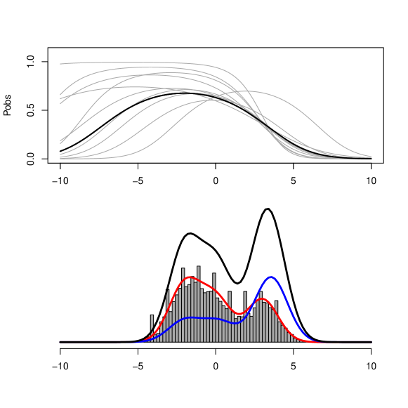
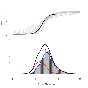
The top panel of Figure 1 shows the true missingness mechanism used to simulate data, as a bold black line. The bottom panel shows a histogram of draws from the observed data as well as the true observed, missing and complete data densities for the continuous component. For this simulation study, we will assume that the relevant estimands are the complete data mean and complete data standard deviation.

Figure 1: Top: the true missingness mechanism (black) and 10 samples from the prior distribution specified in Section 4.1.1 (gray). Bottom: the observed data histogram (gray, $N=10,000$) with observed (red) and missing data (blue) densities for the continuous component. Ten percent of the observed data comes from a discrete distribution on {-4,-3,…,0,…,3,4}.

4.1.1 Analysis using Tukey’s representation

Here we use Tukey’s representation to estimate the posterior distribution of the complete data mean and standard deviation, from observations and observation indicators generated from the model above. In order to do so, we specify prior distributions for the parameters of the missingness mechanism, $\beta$, the fraction of missing data, $Q$, and a model for the observed data, $f^{\rm obs}$.

We posit the following prior distributions on the parameters of the missingness mechanism,

$$\beta_{1} \sim \text{Normal }(-2;2)$$

$$\beta_{2} \sim 0.08\cdot\text{Beta }(3;1)$$

$$Q \sim \text{Uniform }(0,1)$$ (16)

These prior distribution are centered around the parameters of the true missingness mechanism, $(\beta_{1},\beta_{2})$, with some variability to reflect a degree of uncertainty. Importantly, neither $\beta_{1}$ nor $\beta_{2}$ can be estimated from the observed data, and thus the uncertainty in this prior specification will propagate to the posterior, regardless of the amount of observed data. The top panel of Figure 1 shows a number of draws from the above prior distributions, in gray.

Next, we posit the following prior distributions for the observed data parameters, $\theta_{Y|R=1}$:

$$p_{i} \sim \text{Dirichlet}(1,1,\ldots,1)\hbox{ for }i=1,\dots,M=9$$

$$\mu_{k} \sim \text{Normal}(0,10)\hbox{ for }k=1,\dots,K=3$$

$$w_{k} \sim \text{Dirichlet}(1,1,1)$$

$$\sigma_{k} \sim \text{Uniform}(0,2)$$ (17)

Unlike the prior specification for the parameters of the missingness mechanism, all of the observed data parameters are estimable. Thus, the results are only sensitive to the prior specifications of $\theta_{Y|R=1}$ for smaller observed data sample sizes.

Note that by the integrability condition stated in Section 3.1, in order for the continuous mixture components of the complete data to all have positive variance, it must hold that $\beta_{2}<\underset{k=1\dots K}{\text{min}}~{}\frac{1}{2\sigma_{k}^{2}}~{}.$ This inequality is due to Equation 33 in Appendix A.1. To ensure the integrability condition is satisfied, we also bound the prior distributions on $\sigma_{1:3}$ above by 2, because $0.08<\frac{1}{8}$, where $0.08$ is the maximum value of $\beta_{2}$ under our prior distribution.

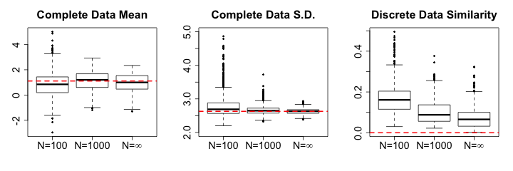
We present the simulation results for different sample sizes in Figure 2. With a reasonably informative prior distribution for the missingness mechanism, these results show that the analysis with the Tukey’s representation accurately recovers the posterior distributions for the relevant estimands. As the sample size increases, our posterior uncertainty shrinks, but never disappears. This is because even with perfect knowledge of the observed data density, there is no information in the data about the parameters of the missingness mechanism, as mentioned above. Therefore uncertainty about the missingness mechanism propagates to the uncertainty about the complete-data quantities, and is the main source of uncertainty in the posterior when enough data is available. This fact facilitates the sensitivity analysis about the missingness mechanism when using Tukey’s representation.

Figure 2: Posterior estimates of the complete-data mean (left), complete-data standard deviation (middle) and maximum absolute difference between the true and inferred discrete probability masses (right). Dashed red line represents the true complete-data value. As we get more data, estimates of the parameters underlying the observed-data distribution improve, and the posterior concentrates around the true values. However, information about the parameters underlying the selection mechanism does not accumulate, thus posterior uncertainty about the complete-data parameters remains.

Above, we illustrated how data analysis using Tukey’s representation can be applied in a straightforward manner to a complex data generating process. It does not require any explicit assumptions about the complete-data distribution; rather it only requires a reasonable model for the observed data, and plausible assumptions about the selection mechanism. In contrast, there are often significant challenges for data analysis when applying the selection factorization, or pattern mixture factorization, as we now discuss.

4.1.2 Remarks on the use of the selection factorization

Inference under selection factorization models typically require numerical or Monte Carlo integration of the complete data distribution, and hence is computationally and analytically more demanding than both pattern mixture models and Tukey’s representation. For instance, often the missing data density does not take on a simple form, and thus missing data imputation is non-trivial. Finally, it is not obvious that the specified selection factorization model will imply a reasonable fit to the this observed data. This is a fundamental challenge associated with any approach that does not directly model the observed data (Rubin, 2004; Little and Rubin, 2014; Lunagomez and Airoldi, 2014; Mealli and Rubin, 2015). The focus on modeling the observed data explicitly, rather than implicitly via assumptions on the data generating process, is one of the strengths of analyses based on the Tukey’s representation.

Even if we knew the complete data distribution corresponded to a six component mixture of Normal with discrete masses at certain values, it would still be difficult to specify appropriately informed prior distribution for the relevant parameters. Note that in this example, the parameters of the missing data density are a function of the selection parameters (Equation 12). For this reason, specifying independent prior information for the mixture components of the complete data density implicitly adds additional prior information about the parameters of the missingness mechanism. By parameterizing the model in terms of complete data parameters $\theta_{Y}$, we are combining what we don’t have information about ($\theta_{Y|R=0}$) with what we do have information about ($\theta_{Y|R=1}$) (Holland, 1986).

4.1.3 Remarks on the use of the pattern-mixture factorization

The true data generating process described at the beginning of Section 4.1 is specified as a mixture. Thus, at least in principle, the pattern mixture factorization, described in Section 2.2, provides an appropriate way to model the complete data. However, the implied missing data distribution in this example does not correspond to a simple location or scale change of the observed data distribution. Thus, as is common with pattern mixture models, the missing data distribution for this data cannot be represented with a simple between-components location and scale change (as discussed, e.g., in Daniels and Hogan, 2000).

More generally, when the missing data distribution is complicated, it can be difficult to propose plausible, scientifically justifiable prior distributions for the parameters of the missing data density, $\theta_{Y|R=0}$. Perhaps even more problematic is that these parameters often imply smoothness and monotonicity of the selection mechanism, which is not explicitly specified in analyses that use the pattern-mixture factorization.

4.2 Robustness to Misspecification

In Section 4.1.1, we performed the analysis using Tukey’s representation using a family of models that included the true data generating process. In practice, finite mixtures of exponential families can only be expected to approximate the observed data density. Here, we evaluate the robustness of Tukey’s approach in such cases.

We consider data generated under a simple selection factorization model. We assume the complete data is a standard normal, i.e. $\theta_{Y}=(\mu,\sigma)=(0,1)$, and that the selection mechanism logistic, linear in the data $y_{i}$. Under this data generating process, the observed data density is

$$f^{\rm obs}(y_{i}\mid r_{i}=1,\theta_{Y},\theta_{R|Y})\propto\frac{\exp\left(\frac{(y_{i}-\mu)^{2}}{2\sigma^{2}}\right)}{\sigma(1+\exp(-\beta_{0}-\beta_{1}y_{i}))},$$

which cannot be represented as a finite mixture of exponential families.

For the analysis, we again assume the goal is to estimate the complete data mean and standard deviation. We use a mixture of normals to approximate the observed data density but take the parameters of the logistic missingness mechanism, $\theta_{R|Y}=(\beta_{0},\beta_{1})$ to be known exactly. We estimate the posterior distributions for $\mu$ and $\sigma$ for increasing sample sizes and for different values of the selection parameters, $\beta_{1}$. More in detail, in each simulation $\beta_{0}$ is fixed to 1/2, the parameter $\beta_{1}$ takes values 1, 2 and 5, and we replicate the analysis for 100 and 1,000 data points. To increase the realism of the data analysis, we fit a mixture model with 3 components to 100 data points, but we increase the flexibility of the model for the larger sample size by fitting a mixture model with 5 components to 1,000 data points.

(a) Complete Data Mean

(b) Complete Data Standard Deviation

Figure 3: Posterior estimates of the complete data mean and complete data standard deviation as a function of sample size and the slope of the missingness mechanism. Blue dots represent the empirical observed data estimates and the dashed red line corresponds to the true complete data quantity. As the slope, $\beta_{1}$ increases, the observed data density approaches a truncated normal, for which Tukey’s representation is not applicable.

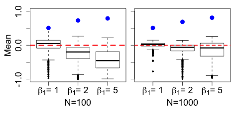
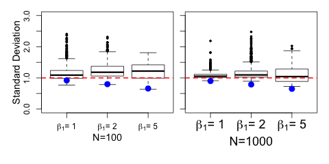
Figure 3 shows box plots of the posterior distributions for the complete data mean (top panels) and complete data standard deviation (bottom panels) for the different values of $\beta_{1}$ and increasing sample sizes. To better appreciate the results, note that, as $\beta_{1}$ increases, the selection probability approaches zero for all $y_{i}<\beta_{0}$ and the observed data density approaches a truncated normal model. Because of the positivity condition, such a model cannot be estimated using Tukey’s representation. The results in Figure 3 show that even when the positivity condition holds, in theory, when the selection probabilities are very close to zero, the complete data estimates (blue dots) become unstable, increasing the bias of the complete data estimates. Thus, in this example, increasing sample size only partially offsets the failure of inference procedures based only on the observed data.

More generally, instability occurs when the odds of selection are small in regions where the inferred observed data density is non-zero. This insight can be formalized by examining the interaction of the observed data density and the selection probabilities in the Equation 24. As a consequence, the fit of the observed data distribution in the tails of the distribution can be very important for accurately inferring complete data quantities. In practice, caution is needed when using Tukey’s representation in cases where the observed data sample size is small or where the selection probabilities diverge rapidly.

4.3 Analysis of transcriptomic and proteomic data

In experiments involving measurements of transcriptomic and proteomic data, mRNA transcripts and proteins which occur at low levels are less likely to be observed (Walther and Mann, 2010; Soon et al., 2013). This makes it challenging to infer normalizing constants for absolute protein levels (Karpievitch et al., 2012), cluster genes into functionally related sets (Troyanskaya et al., 2001), infer the degree of coordination between transcription and translation (Franks et al., 2014), and determine the ratio of dynamic range inflation from transcript to protein levels (Csárdi et al., 2014). Here, we demonstrate how data analysis with Tukey’s representation can be used to investigate some these issues by assessing the sensitivity of estimands to different assumptions about the missingness mechanism.

In this analysis, we use transcriptomic data from Pelechano and Pérez-Ortín (2010), with 14% missing data, and protein abundance data from Ghaemmaghami et al. (2003), with 34% missing data. For illustrative purposes we treat the complete data mean and variance as the estimands of interest in the analysis.

It is standard to assume that both mRNA and protein levels are log-normally distributed (Bengtsson et al., 2005; Lu et al., 2007), although this assumption may not be justified (Lu and King, 2009; Marko and Weil, 2012). Here, we instead model the observed data as a mixture of normals and specify a prior distribution for the parameters of the logistic missingness mechanism. Together these assumptions imply a more flexible prior distribution over complete data densities.

Further, as noted in Karpievitch et al. (2009), missing values can occur for multiple reasons, at different stages of the data collection process. They find that a small fraction of missing proteomic data collected using mass spectrometry is missing completely at random. Consistent with this, we again generalize the results of Section 3.1 to allow the selection mechanism to have a logistic form that asymptotes at some value less than one. The observed data distribution and missingness mechanism together define the joint distribution:

$$f^{\rm obs}(y_{i}|r_{i}=1,\beta,\kappa,\mu_{k},\sigma_{k}) \sim\sum_{k=1}^{K}w_{k}N(y_{i};\mu_{k},\sigma_{k}^{2})$$ (18)

$$f(r_{i}=1|y_{i},\theta_{R|Y}) =\frac{\kappa e^{\beta_{1}y_{i}+\beta_{0}}}{1+e^{\beta_{1}y_{i}+\beta_{0}}}$$ (19)

with $\theta_{Y|R=1}=(\mu,\sigma,w)$ and $\theta_{R|Y}=(\beta_{0},\beta_{1},\kappa)$. Here, $0<(1-\kappa)<1$ corresponds the fraction of data that is missing completely at random, and $\beta_{0}$ and $\beta_{1}$ describe the odds of a missing value, with $\beta_{1}$ parametrizing the rate at which the odds of a missing value change in $y_{i}$. Under this model, the implied missing data distribution is

$$f^{\rm miss}(y_{i}|r_{i}=0,\beta,\kappa,\mu_{k},\sigma_{k}) =(1-\kappa^{*})f^{\rm obs}(y_{i}|r_{i}=1,\mu_{k},\sigma_{k})$$

$$+\kappa^{*}\left(\sum_{k=1}^{K}w_{k}^{*}N(y_{i};\mu_{k}+\beta_{1}\sigma_{k}^{2},\sigma_{k}^{2})\right)$$ (20)

The full derivation of the mixture weights $w^{*}_{k}$ and $\kappa^{*}$ is given in Appendix A.2.

In the analysis of the observations, to poist a good model for $f^{\rm obs}$ in Tukey’s representation, we found that $K=3$ components were enough to approximate the observed data well. Furthermore, we chose the following prior distributions for Q and $\theta_{R|Y}$,

$$\beta_{1} \sim {\rm Beta}(1,3)$$

$$Q \sim {\rm Uniform}(0,1)$$

$$\kappa \sim 1-(1-Q){\rm Beta}(2,1),\quad\kappa\geq Q$$ (21)

Note that $\kappa$ must be greater than $Q$ because the selection probabilities cannot be less than the population fraction of observed data. Draws from this prior distribution are shown in Figure 4, top-left panel, in grey, around the prior mean, in black. We implemented the sampler for the making inference with this model using STAN (Stan Development Team, 2014).

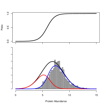
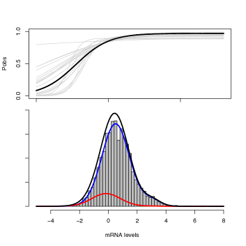
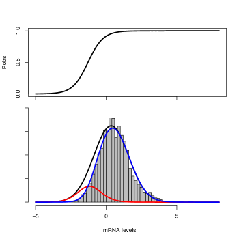
Figure 4, bottom-left panel, shows the fit to the protein data (Ghaemmaghami et al., 2003), when $\beta_{1}$ is set to its median posterior value. For comparison, the bottom-right panel, shows the fit of the selection factorization model published in Franks et al. (2014), which assumes the complete data is distributed according to a lognormal and the missingness mechanism is logistic, with the mean linear in in $y_{i}$. The black, red and blue lines, in both bottom panels, correspond to the estimated densities of complete data, missing data and observed data, respectively. Lack-of-fit to the observed data is the analysis with the selection model. Figure 5 shows the corresponding results for the transcript data set (Pelechano and Pérez-Ortín, 2010), where the lack-of-fit using the selection factorization is less pronounced.

Figure 4: Model fit to proteomic data from Ghaemmaghami et al. (2003) data using two different approaches: Tukey’s representation (left) and the selection factorization (right). The grey lines in the top-left panel represent draws of the selection mechanism from the prior distribution provided in Equation 4.3. The black, red and blue lines in the bottom panels correspond to the estimated densities of complete data, missing data and observed data, respectively.

Figure 5: Model fit to mRNA data from Pelechano and Pérez-Ortín (2010) data using two different approaches: Tukey’s representation (left) and the selection factorization (right). The grey lines in the top-left panel represent draws of the selection mechanism from the prior distribution provided in Equation 4.3. The black, red and blue lines in the bottom panels correspond to the estimated densities of complete data, missing data and observed data, respectively.

In Figures 6–7, we compare the estimated complete data posterior means and standard deviations for the protein and transcript data sets, respectively, using three different missing data models: Tukey’s representation model implied by Equations 18 and 4.3; a selection factorization model that assumes log-normality of the complete data and a logistic selection mechanism (Franks et al., 2014; Csárdi et al., 2014); and a missing complete at random model. For both data sets, the estimates obtained with the MCAR model and with the selection factorization models bookend the estimates obtained with the model specified with Tukey’s representation. Under the selection factorization model, the complete data standard deviation is large and the mean is small relative to the estimates from Tukey’s factorization. This is likely because the strong parametric assumptions associated with the selection factorization models overly constrain the fit to the observed data. Table 1 reports exact numerical estimates of the two estimands of interest, using the three competing models.

Figure 6: Posterior distributions of the complete data mean (right) and complete data standard deviation (left) for protein data (Ghaemmaghami et al., 2003). The MCAR estimates (red) and an estimate assuming normality of the complete data (blue) are shown as vertical lines for comparison. Under the prior distribution in Equation 4.3, estimates using the MCAR and the selection factorization models are at opposite ends of these posterior distributions.

Figure 7: Posterior distributions of the complete data mean (right) and complete data standard deviation (left) for mRNA data (Pelechano and Pérez-Ortín, 2010). The MCAR estimates (red) and an estimate assuming normality of the complete data (blue) are shown as vertical lines for comparison. Under the prior distribution in Equation 4.3, estimates using the MCAR and the selection factorization models are at opposite ends of these posterior distributions.

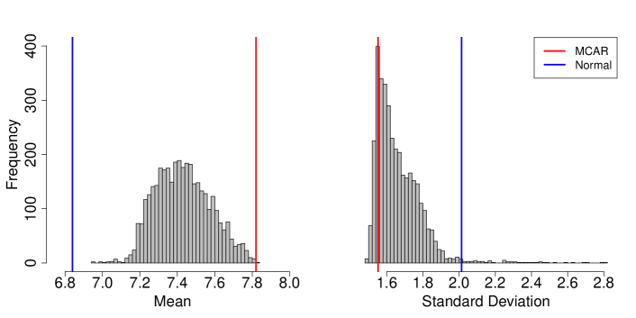
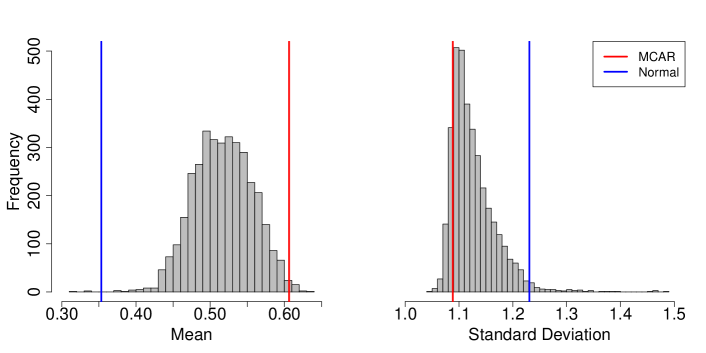
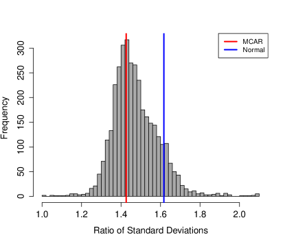
Recent published analyses of data using the selection factorization found that translational regulation widens the dynamic range of protein expression (Franks et al., 2014; Csárdi et al., 2014). One way to quantify the relative dynamic ranges of mRNA and protein is by computing the ratio of the standard deviations between log-mRNA and log-protein levels, a protein-specific quantity often referred to as the “dynamic range ratio”. A value of this ratio less then one suggests that the dynamic range of protein levels is smaller than that of mRNA, and is taken as evidence of a suppressive role of translational regulation. A value greater than one is taken as evidence of amplification, as claimed by the recent analyses.

We used posterior estimates of the complete data standard deviations, obtained from the three competing models fit to both protein and mRNA data sets (Pelechano and Pérez-Ortín, 2010; Ghaemmaghami et al., 2003) to estimate the distribution of the dynamic range ratios, in Figure 8. The results obtained with Tukey’s representation are consistent with those reported by Csárdi et al. (2014), suggesting that translational regulation reflects amplification of protein levels. Table 1 also reports numerical estimates of the the dynamic range ratios.

Estimand	Tukey’s representation	Selection factorization	MCAR	Data set
Mean	7.42  (7.18, 7.73)	6.84	7.82	Prot.
Std. Dev.	1.66  (1.52, 1.94)	2.01	1.55	Prot.
Mean	0.51  (0.44, 0.59)	0.35	0.60	mRNA
Std. Dev.	1.13  (1.07, 1.23)	1.23	1.08	mRNA
Ratios	1.48  (1.28, 1.73)	1.62	1.43	Both

Table 1: Estimates for the quantities of interest obtained with different models, from protein and mRNA data. The dynamic range ratios are computed using both data sets. We report maximum likelihood point estimates for both the MCAR and selection models. We report posterior medians and 95% posterior intervals (in parentheses) for Tukey’s representation.

Figure 8: Dynamic range ratios obtained using Tukey’s representation (histogram), the selection factorization model (blue) of Csárdi et al. (2014), and an MCAR model (red).

These results demonstrate the relative ease of applied data analysis with Tukey’s representation models, and the increased flexibility of models specified using this full conditional specification. By directly modeling the observed data, we avoid the need for Monte Carlo integration of the missing data, and do not require parametric specifications for the complete data density as is typical for selection models. By modeling the selection function directly, we are also able to express uncertainty about the missing data density beyond the simple location and scale changes typical in pattern-mixture model sensitivity analyses.

5 Discussion

Tukey’s representation provides a powerful alternative for specifying missing data models. It allows analysts to eschew some difficult questions about identifiability in models for non-ignorable missing data (Miao et al., 2015) by factoring the joint distribution of the complete-data, $Y$, and missing-data indicators, $R$, in such a way that the missingness mechanism is the only component that must rely on assumptions unassailable using observed data.

5.1 Theoretical insights

Thus far we largely worked with exponential-family models. Here, we make formal statements about exponential family, and give results that hold in greater generality.

Theorem 1.

The normalizing constant $Q$ is the population fraction of observed data.

The proof is straightforward because

$$\mathbb{E}[r_{i}\mid\theta_{Y|R},\theta_{R|Y}] = f(r_{i}=1\mid\theta_{Y|R},\theta_{R|Y})$$

$$= \int f(y_{i},r_{i}=1\mid\theta_{Y|R},\theta_{R|Y})~{}dy_{i}$$

$$= Q(\theta_{Y|R},\theta_{R|Y})~{}\int f^{\rm obs}(y_{i}\mid\theta_{Y|R})~{}dy_{i}$$

$$= Q$$

The density of the observed values, $y^{\rm obs}$ and $r$, can be written in terms of the population fraction of the observed data, $Q$, in full generality,

$$f(y^{\rm obs},r\mid\theta_{R|Y},\theta_{Y|R}) = \prod_{\{i:r_{i}=1\}}f^{\rm obs}(y_{i}\mid\theta_{Y|R})~{}Q\times$$ (23)

$$\times\prod_{\{i:r_{i}=0\}}\int\frac{f(r_{i}=0\mid y_{i},\theta_{R|Y})}{f(r_{i}=1\mid y_{i},\theta_{R|Y})}f^{\rm obs}(y_{i}\mid\theta_{Y|R})~{}Q~{}dy_{i}$$

$$= Q^{\sum_{i}r_{i}}(1-Q)^{N-\sum_{i}r_{i}}\prod_{\{i:r_{i}=1\}}f^{\rm obs}(y_{i}\mid\theta_{Y|R}),$$

using the observation that $\frac{\int\dots\,dy_{i}}{1+\int\dots\,dy_{i}}=1-(1+\int\dots\,dy_{i})^{-1}=1-Q$. And the missing-data density can be expressed as a function of the observed-data density in full generality.

Theorem 2.

The missing-data density can be expressed a function of the observed-data density and the odds of missingness,

$$f^{\rm mis}(y_{i}\mid\theta_{R|Y},\theta_{Y|R})=\frac{Q(\theta_{Y|R},\theta_{R|Y})}{1-Q(\theta_{Y|R},\theta_{R|Y})}\frac{f(r_{i}=0\mid y_{i},\theta_{R|Y})}{f(r_{i}=1\mid y_{i},\theta_{R|Y})}~{}f^{\rm obs}(y_{i}\mid\theta_{Y|R}).$$ (24)

This result can be derived from from the complete-data likelihood and the formula for $Q$ in Equations 4 and 5.

When the missingness mechanism, $f(r_{i}\mid y_{i},\theta_{R|Y})$ does not depend on $y_{i}$, the distribution of the missing data is directly proportional to the distribution of the observed data. Equation 24 can help assess the plausibility of different missingness mechanisms—not at random, completely at random, and at random (Mealli and Rubin, 2015)—by viewing them as functions of the odds of a missing value, $\frac{f(r_{i}=0\mid y_{i},\theta_{R|Y})}{f(r_{i}=1\mid y_{i},\theta_{R|Y})}$. For instance, when the odds have low variance, it may be reasonable to assume the missing data mechanism is completely at random, or at random.

Equation 24 also leads to a general understanding of the main result of Section 3.1, which can be crystallized in the following statement.

Theorem 3.

If the observed-data distribution, $f^{\rm obs}$, belongs to an exponential family, and the log-odds of a missing value are linear in the natural sufficient statistics of that observed-data distribution, then the missing-data distribution, $f^{\rm mis}$, must have the same exponential family as the observed data distribution.

This result can be immediately extended to mixtures.

Corollary 4.

If the observed-data distribution, $f^{\rm obs}$, can be expressed as a $K$-component mixture of an exponential family distribution, and the log-odds of a missing value are linear in the natural sufficient statistics of that observed-data distribution, then the implied missing-data distribution, $f^{\rm mis}$, must be a $K$-component mixture of the same exponential family.

We conjecture that a similar relation might hold outside exponential family models.

5.2 A note on the integrability condition

Not all integrable specifications for $f^{\rm obs}(y_{i}\mid\theta_{Y|R=1})$ and $f(r_{i}\mid y_{i},\theta_{R|Y})$ imply a proper distribution for $f^{\rm mis}(y_{i}\mid\theta_{Y|R=1},\theta_{R|Y})$. In the setting we consider in Section 3, the integrability condition requires the sum $\theta_{Y|R=1}+\theta_{R|Y}$ to lie in the natural parameter space of the exponential family. In practice, analysts may want to consider missing data mechanisms that involve a richer set of parameters, $\tilde{\theta}_{R|Y}$, such as including an intercept, as we illustrate in the context of a biology application, in Section 4.3. In such cases, $\theta_{R|Y}$ is taken to denote the subset of parameters in $\tilde{\theta}_{R|Y}$ that multiply the sufficient statistics of $f^{\rm obs}$. The derivations in Section 3 are simple to repurpose for this situation, accordingly.

For example, assume that the natural parameter $\theta_{Y|R=1}=\eta$, and that the missing data mechanism is logistic with extended parameter vector $\tilde{\theta}_{R|Y}=(\beta_{0},\beta_{1})=(\beta_{0},\theta_{R|Y})$ and $f(r_{i}=1\mid y_{i},\beta)=(1+e^{-(\beta_{0}+T(y_{i})\beta_{1})})^{-1}$. Then, Equations 8 and 9 become

$$Q(\eta,\beta) =\frac{g(\eta+\beta_{1})}{g(\eta+\beta_{1})+g(\eta)e^{\beta_{0}}}$$ (25)

$$f^{\rm mis}(y\mid\eta,\beta) =h(y)g(\eta+\beta_{1})e^{{T(y)}^{\prime}(\eta+\beta_{1})}.$$ (26)

The class of exponential-logistic models defined in Equations 6–7 can be further generalized in two useful ways while maintaining its desirable properties. For instance, generalizing $f^{\rm obs}$ to be a mixture of exponential families as in Section 4.1 is straightforward, and does not increase computation substantially. Relaxing assumptions about the missingness mechanism can be more difficult. Still, it is possible to model $f(r_{i}\mid y_{i},\theta_{R|Y})$ with a mixture of logistic functions, including a missingness mechanism where a fraction of the data is missing completely at random as in Section 4.3.

5.3 Inference strategies

Recall the simple Normal-logistic model of Section 3.2,

$$f(r_{i}=1\mid y_{i},\beta) = \hbox{logit }(\beta_{0}+\beta_{1}y_{i})=\bigm{(}1+\exp\{-\beta_{0}-\beta_{1}y_{i}\}\bigm{)}^{-1}$$

$$f^{\rm obs}(y_{i}) = \hbox{Normal }(0,1).$$

The inferential strategy proposed was to posit prior distributions on $\beta_{1}$ and $Q$, and solve for $\beta_{0}$ at each iteration of the Markov Chain Monte Carlo sampler. A conceptually simpler approach to inference would be to place a prior distribution on all the parameters of the missingness mechanism, and solve for the implied $Q$ at each iteration of the sampler.

In situations where the number of missing values is itself missing, as with truncated data, specifying a prior distribution for all the parameters of the missingness mechanism would lead to an implied prior distribution for the unknown number of missing values, or equivalently, the population fraction of observed data Q.

Figure 9: The region of positive support for the likelihood, restricted to the parameters of the missingness mechanism, is increasingly constrained as the population fraction of missing data $Q$ is estimated with increasingly high precision. This intuition is illustrated by the width of the ridge, which is a function of the amount of information about the fraction of missing data $Q$. We simulated data from a standard Normal distribution and a logistic missingness mechanism. The parameters $(\beta_{0},\beta_{1})$ were set to get 90 percent missing data. The sample size determines the amount of information: $N=100$ (left) and $N=1000$ (right).

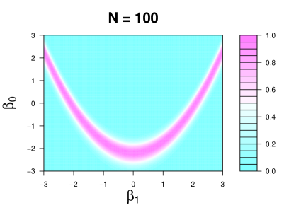
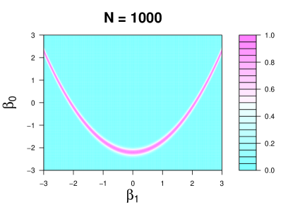
In situations where the number of missing values is known, however, as with censored data, and therefore $Q$ can be estimated from observed data, the support of the likelihood is a constrained parameter space, and a number of choices for the prior distribution on $\beta=\theta_{R|Y}$ would lead to a posterior distribution that is challenging to explore using Monte Carlo methods. Specifically, Equation 5.1 induces a moment constraint that restricts the region where the parameters of the missingness mechanism have positive support to a lower dimensional ridge. Figure 9 illustrates this phenomenon for the simple Normal-logistic model, and increasing sample size.

Sequential Monte Carlo and other specialized Monte Carlo methods that exploit the geometry of the support of posterior distribution may provide a solution in this situation (Doucet et al., 2001; Liu, 2008; Girolami and Calderhead, 2011; Airoldi and Haas, 2011).

5.4 Concluding remarks

In this paper, we used logistic-exponential family models to illustrate how Tukey’s representation can be used to encode non-monotonicity in the missingness mechanism, and to model data with complex distributional forms. These models could also be used to facilitate tipping point analyses (Liublinska and Rubin, 2014), or to incorporate subjective model uncertainty via prior distributions on the missingness mechanism (Rubin, 2004).

Tukey’s representation is most useful when positing reasonable prior distributions on the selection mechanism is feasible. Translating expert knowledge or expectations into a functional form can be challenging, in general, and a logistic missingness mechanism is not always a good choice. In practice, Tukey’s representation should be used in concert with strategies for expert prior elicitation (O’Hagan et al., 2006; Kynn, 2005; Paddock and Ebener, 2009). Nevertheless, prior elicitation for Tukey’s representation is simpler than for other factorizations, since it involves only the set of parameters $\theta_{R|Y}$. In contrast, the selection factorization requires additional assumptions about the complete data density.

In many settings, like the example presented in Section 4.3, we may be able to collect data which partially informs the specification for the selection mechanism. As such, when possible, we can design experiments to learn about the functional form of $f(r_{i}|y_{i},\theta_{R|Y})$ as well as to further refine prior distributions for $\theta_{R|Y}$. Along these lines, Tukey’s representation may be useful in the context of multiphase inference, which is intimately related to problems in missing data (Blocker and Meng, 2013). In these problems, when preprocessing data, it is often the case that we have strong knowledge (or control) of the missingness mechanism yet a weaker understanding of the underlying scientific model.

All in all, we argue that Tukey’s representation, which represents a hybrid of the selection and pattern mixture models is an under-researched yet promising alternative for modeling non-ignorable missing data.

Appendix A Detailed derivations

A.1 Derivations From Section 4.1

First, assume the observed data are normally distributed. For the $k$-th normal component expressed in exponential family form, with natural parameters $\theta_{Y|R=1}$, we have:

$$\theta_{Y|R=1} =(\eta_{1},\eta_{2})=(\frac{\mu_{k}}{\sigma_{k}^{2}},-\frac{1}{2\sigma_{k}^{2}})$$ (27)

$$T(y_{i}) =(y_{i},y_{i}^{2})$$ (28)

$$g(\theta_{Y|R=1}) =\frac{1}{\sqrt{-2\eta_{2}}}e^{\frac{\eta_{1}^{2}}{4\eta_{2}^{2}}}$$ (29)

where $\bm{\mathbf{\eta}}$ are the natural parameters, $\bm{\mathbf{T}}(y)$ the sufficient statistics and $g(\bm{\mathbf{\eta}})$ is the partition function. By Equation 4.1 the odds of a missing value are

$$\frac{f(r_{i}=0|y_{i},\theta_{R|Y})}{f(r_{i}=1|y,\theta_{R|Y})}=\beta_{2}y_{i}^{2}-2\beta_{2}\beta_{1}y_{i}+\beta_{2}\beta_{1}^{2}+\beta_{0}$$ (30)

with $\theta_{R|Y}=(\beta_{0},\beta_{1},\beta_{2})$. Finally, by Equation 9 the implied missing data distribution for the $k$-th component is normal with natural parameters

$$(\eta_{1}^{*},\eta_{2}^{*})=(\eta_{1}-2\beta_{2}\beta_{1},\eta_{2}+\beta_{2})$$ (31)

The inverse parameter mapping for the normal specifies that

$$(\mu_{k},\sigma_{k}^{2})=\left(\frac{-\eta_{1}}{2\eta_{2}},\frac{-1}{2\eta_{2}}\right)$$ (32)

and thus the moments of the missing data distribution are

$$(\mu_{k}^{*},\sigma_{k}^{*2}) =\left(\frac{\frac{-\mu_{k}}{\sigma_{k}^{2}}+2\beta_{2}\beta_{1}}{2(\frac{-1}{2\sigma_{k}^{2}}+\beta_{2})},\frac{-1}{2(\frac{-1}{2\sigma^{2}}+\beta_{2})}\right)$$ (33)

$$=\left(\frac{\mu_{k}-2\beta_{1}\beta_{2}\sigma_{k}^{2}}{1-2\beta_{2}\sigma_{k}^{2}},\frac{\sigma_{k}^{2}}{1-2\beta_{2}\sigma_{k}^{2}})\right)$$

We now extend the results of Section 3.1 to mixture models. First, by Equation 9, the observed data distribution is a mixture of exponential families, the missing data distribution is also a mixture of those same exponential families. By applying Equation 8 to a mixture of exponential families (specifically a mixture of normal and discrete distributions), we have

$$Q(w,\eta,\beta) =\frac{1}{1+\int\left[\alpha\sum_{k}^{K}w_{k}h(y)g(\eta_{k})e^{\eta_{k}T(y)}+(1-\alpha)\sum_{j}^{m}e^{logp_{j}}\right](e^{(\beta_{2}y^{2}-2\beta_{2}\beta_{1}y+\beta_{2}\beta_{1}^{2}+\beta_{0})})}$$

$$=\frac{1}{1+e^{\beta_{0}+\beta_{2}\beta_{1}^{2}}\left[\alpha\sum_{k}^{K}w_{k}\frac{g(\eta_{k})}{g(\eta_{k}^{*})}+(1-\alpha)\sum_{j}^{m}h(p_{j},\gamma_{j},\beta)\right]}$$ (34)

We invert this equation to express $\beta_{0}$ as a function of $Q$, $\eta$ and $(\beta_{1},\beta_{2})$:

$$\beta_{0}(Q,w,\eta,\beta_{1},\beta_{2}) =log\left(\frac{1-Q}{Q\left[\alpha\sum_{k}^{K}w_{k}\frac{g(\eta_{k})}{g(\eta_{k}^{*})}+(1-\alpha)\sum_{j}^{m}h(p_{j},\gamma_{j},\beta)\right]}\right)-\beta_{2}\beta_{1}^{2}$$ (35)

with $h(p_{j},\gamma_{j},\bm{\mathbf{\beta}})=e^{\text{log}p_{j}+\beta_{2}(\gamma_{j}-\beta_{1})^{2}}$. Using Equation 24, we can show that the mixture weights are simply

$$w_{k}^{*} =\frac{w_{k}\frac{g(\eta_{k})}{g(\eta_{k}^{*})}}{\sum_{k}^{K}w_{k}\frac{g(\eta_{k})}{g(\eta_{k}^{*})}}$$ (36)

$$\alpha^{*} =\frac{\alpha\sum_{k}^{K}w_{k}\frac{g(\eta_{k})}{g(\eta_{k}^{*})}}{\alpha\sum_{k}^{K}w_{k}\frac{g(\eta_{k})}{g(\eta_{k}^{*})}+(1-\alpha)\sum_{j}^{m}h(p_{j},\gamma_{j},\beta)}$$

Together, Equations 36 , and 33 yield the missing data distribution specified in 12.

A.2 Derivations From Section 4.3

Assume that the observed data can be represented as a mixture of normals, and also that the odds of a missing value can also be represented by a mixture. Specifically, we allow for some missing values to occur completely at random. We posit that,

$$f(r_{i}=1|y,\theta_{R|Y}) =\frac{\kappa e^{\beta_{1}y+\beta_{0}}}{1+e^{\beta_{1}y+\beta_{0}}}$$ (37)

The mechanism is logistic, but asymptotes at some value $\kappa<1$, where $(1-\kappa)$ represents the fraction of the complete data that is missing completely at random. Under this model, the odds of a missing value are

$$\frac{f(r_{i}=0|y,\theta_{R|Y})}{f(r_{i}=1|y,\theta_{R|Y})} =\left(1-\frac{\kappa e^{\beta_{1}y+\beta_{0}}}{1+e^{\beta_{1}y+\beta_{0}}}\right)\frac{1+e^{\beta_{1}y+\beta_{0}}}{\kappa e^{\beta_{1}y+\beta_{0}}}$$ (38)

$$=\frac{1+(1-\kappa)e^{\beta_{1}y+\beta_{0}}}{\kappa e^{\beta_{1}y+\beta_{0}}}$$ (39)

$$=\frac{1}{\kappa}e^{-\beta_{1}y-\beta_{0}}+\frac{1-\kappa}{\kappa}.$$ (40)

From Equation 8 applied to a mixture of normals,

$$Q(\eta,\beta) = \frac{1}{1+\int\sum_{k}^{K}w_{k}h(y)g(\eta)e^{\eta T(y)}(\frac{1}{\kappa}e^{-\beta_{1}y-\beta_{0}}+\frac{1-\kappa}{\kappa})}$$

$$= \frac{1}{1+e^{-\beta_{0}}\left(\sum_{k}^{K}\frac{w_{k}}{\kappa}\frac{g(\eta)}{g(\eta^{*})}\right)+\frac{1-\kappa}{\kappa}}$$

We can invert Equation A.2 to express $\beta_{0}$ as a function of $Q$,$\eta$, $\beta$ and $\kappa$:

$$\beta_{0}(\eta,\beta_{1},\kappa) = -\log\left(\frac{1-Q}{Q}\frac{(1+\frac{1-\kappa}{\kappa})}{\left(\sum_{k}^{K}\frac{w_{k}}{\kappa}\frac{g(\eta)}{g(\eta^{*})}\right)}\right).$$ (42)

Finally using Equation 24 we find that the missing data are a mixture normals with weights

$$\kappa^{*} =\frac{\sum_{k}^{K}w_{k}\frac{g(\eta_{k})}{g(\beta+\eta_{k})}}{\sum_{k}^{K}w_{k}\frac{g(\eta_{k})}{g(\beta+\eta_{k})}+1-\kappa}$$ (43)

$$w_{k}^{*} =\frac{w_{k}\frac{g(\eta_{k})}{g(\eta_{k}^{*})}}{\sum_{k}^{K}w_{k}\frac{g(\eta_{k})}{g(\eta_{k}^{*})}}.$$ (44)

References

- Airoldi and Haas (2011) Airoldi, E. M. and Haas, B. (2011), “Polytope samplers for inference in ill-posed inverse problems,” in Journal of Machine Learning Research, vol. 15 of W&CS (AiStat).
- Andrea et al. (2001) Andrea, R., Scharfstein, D., Su, T.-L., and Robins, J. (2001), “Methods for conducting sensitivity analysis of trials with potentially nonignorable competing causes of censoring,” Biometrics, 57, 103–113.
- Bengtsson et al. (2005) Bengtsson, M., Ståhlberg, A., Rorsman, P., and Kubista, M. (2005), “Gene expression profiling in single cells from the pancreatic islets of Langerhans reveals lognormal distribution of mRNA levels,” Genome research, 15, 1388–1392.
- Besag (1974) Besag, J. (1974), “Spatial interaction and the statistical analysis of lattice systems,” Journal of the Royal Statistical Society. Series B (Methodological), 192–236.
- Birmingham et al. (2003) Birmingham, J., Rotnitzky, A., and Fitzmaurice, G. M. (2003), “Pattern-mixture and selection models for analysing longitudinal data with monotone missing patterns,” Journal of the Royal Statistical Society. Series B: Statistical Methodology, 65, 275–297.
- Blocker and Meng (2013) Blocker, A. W. and Meng, X.-L. (2013), “The potential and perils of preprocessing: Building new foundations,” Bernoulli, 19, 1176–1211.
- Brook (1964) Brook, D. (1964), “On the distinction between the conditional probability and the joint probability approaches in the specification of nearest-neighbour systems,” Biometrika, 481–483.
- Cressie (2011) Cressie, N. (2011), Statistics for spatio-temporal data, Hoboken, N.J: Wiley.
- Csárdi et al. (2014) Csárdi, G., Franks, A., Choi, D. S., Airoldi, E. M., and Drummond, D. A. (2014), “Accounting for experimental noise reveals that mRNA levels, amplified by post-transcriptional processes, largely determine steady-state protein levels in yeast,” bioRxiv.
- Daniels and Hogan (2000) Daniels, M. J. and Hogan, J. W. (2000), “Reparameterizing the pattern mixture model for sensitivity analyses under informative dropout.” Biometrics, 56, 1241–1248.
- Doucet et al. (2001) Doucet, A., de Freitas, N., and Gordon, N. (eds.) (2001), Sequential Monte Carlo Methods in Practice, Springer.
- Franks et al. (2014) Franks, A. M., Csárdi, G., Drummond, D. A., and Airoldi, E. M. (2014), “Estimating a structured covariance matrix from multi-lab measurements in high-throughput biology,” Journal of the American Statistical Association, 00–00.
- Gelman et al. (2004) Gelman, A., Carlin, J., Stern, H., and Rubin, D. B. (2004), Bayesian Data Analysis, Boca Raton: CRC Press.
- Ghaemmaghami et al. (2003) Ghaemmaghami, S., Huh, W. K., Bower, K., Howson, R. W., Belle, A., Dephoure, N., O’Shea, E. K., and Weissman, J. S. (2003), “Global analysis of protein expression in yeast,” Nature, 425, 737–741.
- Girolami and Calderhead (2011) Girolami, M. and Calderhead, B. (2011), “Riemann manifold Langevin and Hamiltonian Monte Carlo methods,” Journal of the Royal Statistical Society. Series B: Statistical Methodology, 73, 123–214.
- Glynn et al. (1986) Glynn, R. J., Laird, N. M., and Rubin, D. B. (1986), “Selection modeling versus mixture modeling with nonignorable nonresponse,” in Drawing inferences from self-selected samples, Springer, pp. 115–152.
- Hammersley and Clifford (1971) Hammersley, J. M. and Clifford, P. (1971), “Markov fields on finite graphs and lattices,” .
- Holland (1986) Holland, P. (1986), “Discussion 4: Mixture Modeling Versus Selection Modeling With Nonignorable Nonresponse,” in Drawing inferences from self-selected samples, ed. Wainer, H., Routledge, pp. 143–149.
- Karpievitch et al. (2009) Karpievitch, Y., Stanley, J., Taverner, T., Huang, J., Adkins, J. N., Ansong, C., Heffron, F., Metz, T. O., Qian, W.-J., Yoon, H., Smith, R. D., and Dabney, A. R. (2009), “A statistical framework for protein quantitation in bottom-up MS-based proteomics.” Bioinformatics (Oxford, England), 25, 2028–34.
- Karpievitch et al. (2012) Karpievitch, Y. V., Dabney, A. R., and Smith, R. D. (2012), “Normalization and missing value imputation for label-free LC-MS analysis,” BMC bioinformatics, 13, S5.
- Kynn (2005) Kynn, M. (2005), “Eliciting expert knowledge for Bayesian logistic regression in species habitat modelling,” .
- Little (1993) Little, R. J. (1993), “Pattern-mixture models for multivariate incomplete data,” Journal of the American Statistical Association, 88, 125–134.
- Little and Rubin (2014) Little, R. J. and Rubin, D. B. (2014), Statistical analysis with missing data, John Wiley & Sons.
- Liu (2008) Liu, J. S. (2008), Monte Carlo Strategies in Scientific Computing, Springer, 2nd ed.
- Liublinska and Rubin (2014) Liublinska, V. and Rubin, D. B. (2014), “Sensitivity analysis for a partially missing binary outcome in a two-arm randomized clinical trial.” Statistics in medicine, 33, 4170–85.
- Lu and King (2009) Lu, C. and King, R. D. (2009), “An investigation into the population abundance distribution of mRNAs, proteins, and metabolites in biological systems,” Bioinformatics, 25, 2020–2027.
- Lu et al. (2007) Lu, P., Vogel, C., Wang, R., Yao, X., and Marcotte, E. M. (2007), “Absolute protein expression profiling estimates the relative contributions of transcriptional and translational regulation,” Nature biotechnology, 25, 117–124.
- Lunagomez and Airoldi (2014) Lunagomez, S. and Airoldi, E. (2014), “Valid inference from non-ignorable network sampling designs,” arXiv no. 1401.4718.
- Marko and Weil (2012) Marko, N. F. and Weil, R. J. (2012), “Non-Gaussian Distributions Affect Identification of Expression Patterns, Functional Annotation, and Prospective Classification in Human Cancer Genomes,” PloS one, 7, e46935.
- Mealli and Rubin (2015) Mealli, F. and Rubin, D. B. (2015), “Clarifying missing at random and related definitions, and implications when coupled with exchangeability,” Biometrika, in press.
- Miao et al. (2015) Miao, W., Ding, P., and Geng, Z. (2015), “Identifiability of Normal and Normal Mixture Models With Nonignorable Missing Data,” .
- Molenberghs et al. (2015) Molenberghs, G., Fitzmaurice, G. M., Kenward, M. G., Tsiatis, A. A., and Verbeke, G. (eds.) (2015), Handbook of Missing Data Methodology, Chapman & Hall/CRC Press.
- O’Hagan et al. (2006) O’Hagan, A., Buck, C. E., Daneshkhah, A., Eiser, J. R., Garthwaite, P. H., Jenkinson, D. J., Oakley, J. E., and Rakow, T. (2006), Uncertain judgements: eliciting experts’ probabilities, John Wiley & Sons.
- Paddock and Ebener (2009) Paddock, S. M. and Ebener, P. (2009), “Subjective prior distributions for modeling longitudinal continuous outcomes with non-ignorable dropout,” Statistics in medicine, 28, 659–678.
- Pelechano and Pérez-Ortín (2010) Pelechano, V. and Pérez-Ortín, J. E. (2010), “There is a steady-state transcriptome in exponentially growing yeast cells,” Yeast, 27, 413–422.
- Robert and Casella (2004) Robert, C. P. and Casella, G. (2004), Monte Carlo Statistical Methods, Second Edition, Springer-Verlag.
- Rubin (1977) Rubin, D. (1977), “Formalizing Subjective Notions About The Effect on Nonrespondents in Sample Surveys,” Journal of the American Statistical Association.
- Rubin (1974) Rubin, D. B. (1974), “Characterizing the estimation of parameters in incomplete data problems,” Journal of the American Statistical Association, 69, 467–474.
- Rubin (1976) — (1976), “Inference and Missing Data,” Biometrika, 63, 581.
- Rubin (1978) — (1978), “Bayesian inference for causal effects: The role of randomization,” Annals of Statistics, 6, 34–58.
- Rubin (2004) — (2004), Multiple Imputation for Nonresponse in Surveys, Wiley Classic Library.
- Scharfstein et al. (1999) Scharfstein, D. O., Rotnitzky, A., and Robins, J. M. (1999), “Adjusting for Nonignorable Drop-Out Using Semiparametric Nonresponse Models,” Journal of the American Statistical Association, 94, 1096–1120.
- Soon et al. (2013) Soon, W. W., Hariharan, M., and Snyder, M. P. (2013), “High-throughput sequencing for biology and medicine,” Molecular Systems Biology, 9.
- Stan Development Team (2014) Stan Development Team (2014), “Stan: A C++ Library for Probability and Sampling, Version 2.2,” .
- Troyanskaya et al. (2001) Troyanskaya, O., Cantor, M., Sherlock, G., Brown, P., Hastie, T., Tibshirani, R., Botstein, D., and Altman, R. B. (2001), “Missing value estimation methods for DNA microarrays,” Bioinformatics, 17, 520–525.
- Walther and Mann (2010) Walther, T. C. and Mann, M. (2010), “Mass spectrometry–based proteomics in cell biology,” The Journal of Cell Biology, 190, 491–500.