A HIGH-PRECISION NEAR-INFRARED SURVEY FOR RADIAL VELOCITY VARIABLE LOW-MASS STARS USING CSHELL AND A METHANE GAS CELL

Abstract

We present the results of a precise near-infrared (NIR) radial velocity (RV) survey of 32 low-mass stars with spectral types K2–M4 using CSHELL at theNASA IRTF in the $K$-band with an isotopologue methane gas cell to achieve wavelength calibration and a novel iterative RV extraction method. We surveyed 14 members of young ($\approx$ 25–150 Myr) moving groups, the young field star $\varepsilon$ Eridani as well as 18 nearby ($<$ 25 pc) low-mass stars and achieved typical single-measurementprecisions of 8–15 m s^-1 with a long-term stability of 15–50 m s^-1 over longer baselines. We provide the first multi-wavelength confirmation of GJ 876 bc and independently retrieve orbital parameters consistent with previous studies. We recovered RV variability for HD 160934 AB and GJ 725 AB that are consistent with their known binary orbits, and nine other targets are candidate RV variables with a statistical significance of 3–5$\sigma$.Our method combined with the new iSHELL spectrograph will yield long-termRV precisions of $\lesssim$ 5 m s^-1 in the NIR, which will allow the detection of Super-Earths near the habitable zone of mid-M dwarfs.

1 INTRODUCTION

The method of Doppler radial velocity (RV) variations has proven itself fruitful in the last decades both for the identification of new exoplanets (e.g., Mayor & Queloz, 1995; Marcy et al., 1998; Delfosse et al., 1998a; Marcy et al., 2001; Cochran et al., 2002; Endl et al., 2003; Butler et al., 2004; Rivera et al., 2005b, 2010; Meschiari et al., 2011; Dumusque et al., 2012; Montet et al., 2014; Tuomi et al., 2014) and the confirmation of exoplanets detected by the method of transit (e.g. Kepler–78b; Sanchis-Ojeda et al., 2013; Pepe et al., 2013; Akeson et al., 2013). Recent developments have shown that cool ($\lesssim$ 3800 K) stellar hosts in the M spectral class represent valuable targets for the identification of new Earth-mass planetary companions in the habitable zone with the RV method due to their smaller mass and significantly larger population (Henry et al., 2006).

However, it becomes gradually harder to obtain sufficient signal-to-noise (S/N) ratios at optical wavelengths at decreasing effective temperatures (Reiners et al., 2010; Bottom et al., 2013). To worsen the case, late-type M dwarfs are on average more active and display more stellar spots (e.g., Shkolnik et al., 2009; Morin et al., 2010; Shkolnik et al., 2012; Malo et al., 2014; Schmidt et al., 2015), which can induce RV signals very similar to those of planetary companions (e.g., Queloz et al., 2001; Paulson & Yelda, 2005). Robertson et al. (2014) demonstrated the importance of a careful consideration of stellar activity in exoplanet searches by demonstrating that the purported GJ 581 d habitable-zone exoplanet (Udry et al., 2007) was most likely a false-positive signal caused by stellar spots. Overcoming this limitation is especially important in the search for very low-mass companions that induce RV variations of low amplitudes (e.g. a few m s^-1) comparable to stellar activity jitter.

The study of RV variations in the regime of near-infrared (NIR) wavelengths addresses both these issues. First, a larger fraction of the flux of cooler ($\lesssim$ 3850 K), later-type ($\gtrsim$ M0; Pecaut & Mamajek 2013) host stars is emitted at these wavelengths, although care must be used in choosing the observed NIR wavelength range for M0–M4 dwarfs as their lack of spectral features can counterbalance the brightness advantage (Reiners et al., 2010).

Secondly and perhaps more importantly, the RV signal induced by stellar spots is expected to have an $\approx\lambda^{-1}$ dependence for modest spot contrast temperatures, where $\lambda$ is the wavelength (Reiners et al., 2010; Anglada-Escudé et al., 2012; Howard et al., 2013; Pepe et al., 2013; Plavchan et al., 2015; Marchwinski et al., 2015), which means that the effect of stellar spots on NIR RV measurements is less important than it is at visible wavelengths by a factor $\sim$ 4. Furthermore, the RV signal induced on a stellar host by a substellar companion via the Doppler effect is wavelength-independent, hence a multi-wavelengths RV follow-up opens the possibility of rejecting exoplanet candidates that are caused by other astrophysical phenomena that would cause RV variations of different amplitudes in the optical and NIR regimes.

RV surveys in the NIR are still trailing behind their optical counterparts in terms of long-term RV stability, with best reported NIR results at $\approx$ 5 m s^-1 (Bean et al., 2010) using 8 m-class telescopes, or $\approx$ 45–60 m s^-1 (Blake et al., 2010; Crockett et al., 2011; Tanner et al., 2012; Bailey et al., 2012) using smaller facilities, versus 0.8–15 m s^-1 in the optical (Cochran & Hatzes, 1994; Kürster et al., 1994; Endl et al., 2006; Mayor & Udry, 2008; Howard et al., 2010b; Dumusque et al., 2012). This is mainly due to , and technical challenges , given that NIR instrumentation and observing methods have only been developed relatively recently. As an example, iodine gas cells, which have been used extensively as wavelength calibrators in optical RV surveys, do not offer a sufficient density of absorption lines in the NIR domain. For this reason, most existing NIR RV studies have used telluric lines to achieve wavelength calibration (Blake et al., 2010; Crockett et al., 2011; Bailey et al., 2012; Tanner et al., 2012; Davison et al., 2015), with the exception of Bean et al. (2010) who used an ammonia gas cell with CRIRES at the VLT to obtain unprecedented long-term precisions of $\approx$ 5–10 m s^-1 in the NIR on targets with $K_{S}$-band magnitudes between 4.4 and 8.0.

Our team has recently developed a methane isotopologue gas cell that offers a high absorption line density in the NIR regime to achieve RV measurements of the order of a few m s^-1 with the limited spectral grasp of CSHELL at the NASA InfraRed Telescope Facility (IRTF; Anglada-Escudé et al., 2012; Plavchan et al., 2013), as well as an iterative algorithm that allows for the simultaneous solving of the wavelength solution, the construction of an empirical stellar spectrum and the measurement of stellar RVs (P. Gao et al., submitted to PASP). In this paper, we present the results of a NIR RV survey of 32 late-type, nearby stars using CSHELL at the IRTF using this new RV extraction pipeline. We achieve long-term single-measurement high-S/N RV precisions of $\approx$ 8 m s^-1 within a single night and $\approx$ 15 m s^-1 over long-term baselines up to several years, which represents a substantial improvement over previously reported single-measurements precisions using CSHELL and no gas cell (e.g., 58 m s^-1 within a single night; Crockett et al. 2011; or 90 m s^-1 on baselines of several years; Davison et al. 2015).

In Section 2, we present the method by which we constructed our target sample. The observing setup and strategy is then detailed in Section 3. We summarize the spectral extraction method and the RV measurement algorithm in Sections 4 and 5, respectively. The method by which we combine individual RV measurements is presented in Section 6. Our global survey results are then presented in Section 7, and we discuss individual targets in Section 8. We finally present our conclusions in Section 9.

2 SAMPLE SELECTION

Our survey sample is composed of two parts; the first consists of nearby, young stars mostly selected from known members of young moving groups, and the second consists of nearby ($<$ 25 pc) stars of any age. Comparing our results with those of optical RV surveys for the young sample will eventually allow us to characterize how the signature of stellar activity on RV curves differ between these two wavelength regimes, whereas completing the census of giant close-in planets in a volume-limited sample will be useful to derive population statistics in the near future. In this Section, we describe the process by which these samples were constructed. The complete survey sample is presented in Table 2.2 and a spectral types histogram of it is presented in Figure 1.

2.1 The Young Sample

The young sample was constructed by selecting K to mid M-type young stars in the solar neighborhood, mainly from known members of young moving groups such as $\beta$ Pictoris ($24\pm 3$ Myr; Zuckerman et al., 2001; Bell et al., 2015a), AB Doradus ($149^{+51}_{-19}$ Myr; Zuckerman et al., 2004; Bell et al., 2015a) and the Octans-Near association ($\approx$ 30–100 Myr; Zuckerman et al. 2013), with 2MASS $K_{S}$-band magnitudes brighter than $7.1$ (the brightest target $\varepsilon$ Eridani has $K_{S}=1.8$) so that a S/N of $\sim$ 80 could be achieved within approximately an hour. .

No selection cut was applied on projected rotational velocities; all stars in this sample have measured $v\sin i$ values ranging from 2 to 70 km s^-1. All $<$ 2" binaries were rejected from the sample, except for GJ 3305 AB (0$\farcs$093; Kasper et al. 2007) and HD 160934 AB (0$\farcs$12; Gálvez et al. 2006), which were not known to be binary stars at the time when the young sample was assembled. A total of 15 targets were selected and are listed in Table 2.2, with spectral types ranging from K2 to M4.

Six targets in the young sample had never benefitted from a precise RV follow-up. Six others were already followed either at optical or NIR wavelengths albeit at a $\gtrsim$ 50 m s^-1 precision (AG Tri, AT Mic A, AT Mic B, AU Mic, BD+01 2447, V1005 Ori; Bailey et al., 2012; Paulson & Yelda, 2006), and three targets benefitted from a precise RV follow-up at optical wavelengths (BD+20 1790, $\varepsilon$ Eridani, GJ 3305 AB; e.g., Figueira et al., 2010; Hernán-Obispo et al., 2015; Campbell et al., 1988; Elliott et al., 2014).

.

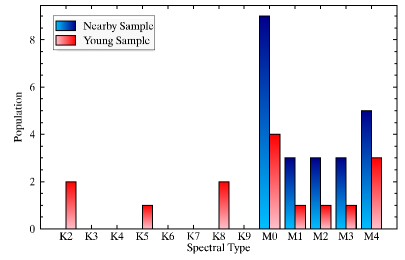
Figure 1: Spectral type histogram of the nearby and young target samples that were studied in this work. Targets that fall into both samples are shown in both histograms (and thus appear twice). For more details, see Section 2

2.2 The Nearby Sample

The nearby sample was constructed by selecting all M dwarfs from the Reserach Consortium on Nearby Stars (RECONS; Henry et al., 2014) and the Lépine and Shara Proper Motion (LSPM) catalog (Lépine, 2005) with a trigonometric distance measurement that places them within 25 pc of the Sun. We avoided including targets that were already part of precise RV follow-up programs, such as the Hobble-Eberly Telescope survey (HET; Endl et al., 2003, 2006), the California Planet Survey (CPS; Howard et al., 2010a; Montet et al., 2014), and the Ultraviolet and Visual Echelle Spectrograph re-analysis of Tuomi et al. (2014). We selected the targets that are easily accessible from the IRTF ($-35$° $<$ DEC $<65$°) with apparent 2MASS magnitudes $K_{S}<6.4$. We used a more conservative $K_{S}$-band cut in this sample to achieve a S/N of at least 200 per pixel within a few hours (see Section 3).

All targets with a known stellar companion or a background star at $<$ 2" were rejected from the sample. We obtained projected rotational velocities ($v\sin i$) from the literature when available and rejected targets with $v\sin i\geq 20$ km s^-1. From this initial list of targets, we followed 21 low-mass stars with spectral types in the M0–M4 range, which are listed in Table 2.2. All of these targets have rotational velocity measurements in the literature, which range from 3 to 16 km s^-1. It can be noted that 4 targets are present in both the nearby and young samples.

Fourteen targets in the nearby sample never had precise RV follow-up observations. Five targets were already followed at NIR wavelengths albeit at a $\gtrsim$ 50 m s^-1 precision (AT Mic A, AT Mic B, AU Mic, EV Lac and GJ 725 A; Bailey et al. 2012), and two other targets benefitted from a precise RV follow-up at optical wavelengths (GJ 15 A and GJ 876; e.g., Delfosse et al., 1998a; Marcy et al., 1998; Rivera et al., 2010; Howard et al., 2014).

Table 1: Precise NIR RVs Follow-Up Sample

Common	RA J2000	DEC J2000	Sp.	Ref.	2MASS	$v\sin i$	Ref.	Binary	Ref.	$\log R^{\prime}_{HK}$	Activity	Ref.
Name	(hh:mm:ss)	(dd:mm:ss)	Type		$K_{S}$	(km s-1)		Sep. (")
Nearby, Young Sample
AT Mic B	20:41:51.147	-32:26:10.22	M4	27	4.94	$15.8\pm 1.2$	12	3.6	$\cdots$	$\cdots$	$\cdots$	$\cdots$
AT Mic A	20:41:51.156	-32:26:06.58	M4	27	4.94	$10.1\pm 1.2$	12	3.6	$\cdots$	$\cdots$	$\cdots$	$\cdots$
AU Mic	20:45:09.492	-31:20:26.66	M1	27	4.53	$9.3\pm 1.2$	12	$\cdots$	$\cdots$	$-4.053\pm 0.057$	VA	11
EQ Peg A	23:31:52.087	19:56:14.22	M3.5	28	5.33	$12.8\pm 5.0$	10	$5.0$	14	($-5.162\pm 0.057$)	(VI)	6
Young Sample
AG Tri	02:27:29.254	30:58:24.61	K8	27	7.08	$5\pm 2$	1	$22.2$	2	$\cdots$	$\cdots$	$\cdots$
$\varepsilon$ Eridani	03:32:55.911	-09:27:29.86	K2	29	1.78	$2.45\pm 0.5$	3	$\cdots$	$\cdots$	$-4.478\pm 0.031$	A	4
V577 Per	03:33:13.491	46:15:26.53	K2	5	6.37	$8.9\pm 0.9$	38	$\cdots$	$\cdots$	$-4.109\pm 0.057$	VA	6
GJ 3305 AB	04:37:37.467	-02:29:28.45	M0	30	6.41	$6.50\pm 0.5$	7	0.093	$\cdots$	$\cdots$	$\cdots$	$\cdots$
TYC 5899–26–1	04:52:24.407	-16:49:21.97	M3	27	6.89	$<3$	5	$\cdots$	$\cdots$	$\cdots$	$\cdots$	$\cdots$
V1005 Ori	04:59:34.831	01:47:00.68	M0	27	6.26	$8.7\pm 0.9$	8	$\cdots$	$\cdots$	$-4.080\pm 0.151$	VA	8
BD+20 1790	07:23:43.592	20:24:58.66	K5	31	6.88	$15.70\pm 3.16$	9	$\cdots$	$\cdots$	$-3.800\pm 0.0037$	VA	8
BD+01 2447	10:28:55.551	00:50:27.62	M2	27	5.31	$0.1\pm 0.2$	10	$\cdots$	$\cdots$	$-5.029\pm 0.057$	I	11
HD 160934 AB	17:38:39.634	61:14:16.03	M0	27	6.81	$19.1\pm 0.6$	8	0.12	$\cdots$	$-3.87\pm 0.120$	VA	8
LO Peg	21:31:01.711	23:20:07.47	K8	27	6.38	$70\pm 10$	10	$\cdots$	$\cdots$	$-3.906\pm 0.050$	VA	13
BD–13 6424	23:32:30.864	-12:15:51.43	M0	27	6.57	$8.8\pm 1.2$	12	$\cdots$	$\cdots$	$\cdots$	$\cdots$	$\cdots$
Nearby Sample
GJ 15 A	00:18:22.885	44:01:22.63	M2	32	4.02	$1.43\pm 0.5$	7	$31.9$	2	$-5.27\pm 0.04$	VI	8
GJ 169	04:29:00.138	21:55:21.48	M0.5	33	4.88	$3.8\pm 1.8$	10	$\cdots$	$\cdots$	$-4.813\pm 0.154$	I	8
LHS 26	04:31:11.479	58:58:37.57	M4	32	5.72	$<3$	15	$8.9$	2	$\cdots$	$\cdots$	$\cdots$
GJ 338 A	09:14:22.982	52:41:12.53	M0	32	3.99	$2.9\pm 1.2$	16	$18.1$	17	$-4.652\pm 0.166$	A	8
GJ 338 B	09:14:24.856	52:41:11.84	M0	32	4.14	$2.8\pm 1.2$	16	$18.1$	17	$-4.420\pm 0.050$	A	18
GJ 458 A	12:12:20.847	54:29:08.69	M0	31	6.06	$5.4\pm 1$	8	$14.7$	20	$-4.970\pm 0.040$	I	8
GJ 537 B	14:02:33.128	46:20:23.92	M0	34	5.39	$<4$	21	$3.0$	$\cdots$	($-4.971\pm 0.057$)	(I)	4
GJ 537 A	14:02:33.240	46:20:26.64	M2	34	5.43	$<4$	21	$3.0$	2	$-4.733\pm 0.057$	A	4
LHS 371	14:25:43.496	23:37:01.06	M0	34	5.97	$<4$	21	$45.4$	20	$\cdots$	$\cdots$	$\cdots$
LHS 372	14:25:46.671	23:37:13.31	M1	34	6.09	$<4$	21	$45.3$	22	$\cdots$	$\cdots$	$\cdots$
LHS 374	14:30:47.794	-08:38:46.57	M0	34	5.77	$<3$	10	$50.0$	23	$-4.896\pm 0.057$	I	24
GJ 9520	15:21:52.919	20:58:39.48	M1.5	31	5.76	$6.5\pm 3$	21	$\cdots$	$\cdots$	$\cdots$	$\cdots$	$\cdots$
GJ 3942	16:09:03.097	52:56:37.95	M0	35	6.33	$<4$	21	$\cdots$	$\cdots$	$\cdots$	$\cdots$	$\cdots$
GJ 725 A	18:42:46.679	59:37:49.47	M3	32	4.43	$<2.5$	26	13.3	$\cdots$	$-5.267\pm 0.229$	VI	11
GJ 740	18:58:00.140	05:54:29.70	M0.5	21	5.36	$3.8\pm 2.8$	8	$\cdots$	$\cdots$	$-4.825\pm 0.175$	I	8
EV Lac	22:46:49.807	44:20:03.10	M3.5	36	5.30	$6.9\pm 0.8$	8	$10.0$	2	$-3.972\pm 0.147$	VA	8
GJ 876	22:53:16.722	-14:15:48.91	M4	37	5.01	$2.8\pm 2.2$	25	$\cdots$	$\cdots$	($-5.146\pm 0.057$)	(VI)	11

Note. — See Section 2 for more details

References. — (1) Cutispoto et al. 2000; (2) Mason et al. 2001; (3) Butler et al. 2006; (4) Duncan et al. 1991; (5) Schlieder et al. 2010; (6) Pace 2013; (7) Houdebine 2010; (8) Herrero et al. 2012; (9) White et al. 2007; (10) Głȩbocki & Gnaciński 2005; (11) Isaacson & Fischer 2010; (12) Torres et al. 2006; (13) Gray et al. 2003; (14) Fabricius et al. 2002; (15) Mohanty & Basri 2003; (16) Delfosse et al. 1998b; (17) Orlov et al. 2012; (18) Eiroa et al. 2013; (19) Stelzer et al. 2013; (20) Lépine & Bongiorno 2007; (21) Reiners et al. 2012; (22) Salim & Gould 2003; (23) Worley & Douglass 1997; (24) Arriagada 2011; (25) Marcy & Chen 1992; (26) Browning et al. 2010; (27) Malo et al. 2013; (28) Davison et al. 2015; (29) Keenan & McNeil 1989; (30) Kasper et al. 2007; (31) Reid et al. 2004; (32) Jenkins et al. 2009; (33) Koen et al. 2010; (34) Gaidos et al. 2014; (35) Vyssotsky 1956; (36) Hawley et al. 1997; (37) Lafrenière et al. 2007; (38) McCarthy & Wilhelm 2014.

Both the HET and CPS catalogs used similar selection criteria with the exception that young and/or chromospherically active systems were rejected. Thus, we are subject to a bias towards these systems despite our rejection of high-$v\sin i$ targets. One target in the sample (GJ 740) has been followed as part of the HARPS survey (Bonfils et al., 2013), but no results were published at the time the target list was assembled, hence we have included it in the sample.

We flag chromospheric activity in Table 2.2 based on $\log{R^{\prime}_{HK}}$ index values from the literature, when available (e.g., see Zirker 1968; Noyes et al. 1984.)

3 OBSERVATIONS

We obtained our data using the NIR high resolution single-order echelle spectrograph CSHELL (Greene et al., 1993; Tokunaga et al., 1990) at the 3 m IRTF from 2010 October to 2015 January. The survey presented here includes a total of 3794 individual spectra obtained in a total of 65 observing nights. We used the 0$\farcs$5 slit and the continuous variable filter, yielding a resolving power of $R=46\,000$ (Crockett et al., 2011; Prato et al., 2015) with a spectral grasp of $\approx$ 5.55 nm at 2.3125 $\mu$m. It is noteworthy to mention that Davison et al. 2015 measured a resolving power as high as $R=57\,000$ with the 0$\farcs$5 slit from modelling observed absorption telluric lines and suggested that this could be due to the slit being slightly narrower than its designation. The spectrograph uses a $\approx$ 25 yr-old 256x256 pixels InSb detector that has a significant number of bad pixels compared to more recent NIR detectors.

A ¹³CH₄ isotopologue methane gas cell (Anglada-Escudé et al., 2012; Plavchan et al., 2013) was inserted in the shutter beam to provide a wavelength reference in the NIR. . The grating angle was set once at the beginning of each night by observing an A-type star and ensuring that the deep methane absorption line of the gas cell at $\approx$ 2.31355 $\mu$m was located on column 179 of the detector to achieve identical wavelength coverage, as the position of the deep methane feature typically varied by $\sim$ 1–2 detector pixels between observing nights. This setup typically corresponded to central wavelength values of $\approx$ 2.31255 $\mu$m.

We obtained science exposures of 300 s or less to avoid saturation or significant background variations, and obtained several exposures (typically $\sim$ 5–60) to achieve a combined S/N of $\sim$ 70 to 200 depending on the survey sample. We did not obtain pair-subtracted spectra as our targets are significantly brighter than background sky emission, and all spectra were obtained with the methane gas cell in beam.

Starting in 2014, we systematically observed one bright A-type star (either Sirius, Castor, Vega, Alphecca, $\beta$ Arietis or 32 Pegasi depending on their altitude) at the beginning of every night to obtain a S/N $\approx 200$ spectrum of the gas cell and characterize any potential long-term variation. Fifteen flat-field exposures of 15 s were initially obtained at the beginning of every night, however starting from 2014 April 2, we obtained fifteen 15 s flat-field exposures after every science target to minimize systematic instrumental effects. We did not apply dark frame calibrations as we found that they did not improve the quality of our results. A log of all observations obtained in this work is presented in Table 2, where S/N values are calculated by assuming that the spectra are photon-noise limited.

Table 2: Log of All Science Star Observations

Target	UT Date	Num. of	Median
Name	(YYMMDD)	Spectra	S/N
AG Tri	101009	6	23
	101011	15	16
	101012	12	23
	101122	12	22
	101123	12	26
	101124	12	20
	110216	9	22
	110219	10	25
	110716	10	20
	110819	14	28
AT Mic A	101010	6	39
	101011	11	35
	101013	10	28
	101123	2	26
	101124	6	43

Note. — See Section 3 for more details.

4 SPECTRAL EXTRACTION

Due to several challenges in extracting RVs out of CSHELL spectra, we constructed our own custom data reduction pipeline to extract the 3794 spectra obtained in this work in a consistent way. We summarize below this data extraction pipeline, which is described in more details in P. Gao et al. (submitted to PASP).

Per-target flat fields were generated by median-combining data sets that each consist of 15 individual files. 2D sinusoidal fringing with amplitude $\sim$ 0.2–0.6% was found to be present in these flat fields due to the CSHELL circular variable filter, which limited our RV precision to $>$ 55 m s^-1 when left uncorrected. Fringing subtraction was thus achieved by median-combining a large number of per-target flat fields spanning several years to obtain a master flat field. This averaged out the fringing due to its spatial and spectral variations over time. Individual per-target flat fields were then normalized by the master flat field to bring out their fringing pattern, which was fitted and corrected individually.

Fringing is also present in the science observations, but similar efforts to correct fringing were not possible due to low illumination of most of the image aside from the spectral trace of the target. Thus, we removed this fringing in the RV extraction process.

Spectral extraction was performed by first dividing the fringing-corrected, per-target flat fields from the science observations, followed by correcting for a linear tilt in the target trace on the detector. A Moffat profile was then fit to the trace in the spatial direction, and the 1D spectrum was extracted using the median trace profile with an optimal extraction procedure (Horne, 1986; Massey & Hanson, 2013). Following this, a synthetic spectral trace was constructed from the extracted spectrum and the spatial profile and was divided out from the observed spectral trace. The 2D residuals resulting from this operation were combed for large deviations from the median, which were flagged as bad pixels. A 1D spectrum was extracted again from the spectral trace after having masked these bad pixels. Additional bad pixels were flagged by noting any major deviations from the continuum in the 1D spectra, in order for them to be ignored by the RV extraction pipeline.

5 RADIAL VELOCITY EXTRACTION

We used a novel forward modelling MATLAB RV pipeline to compute the relative RV of every individual spectrum, which we summarize in this section. The pipeline is described in detail by P. Gao et al. (submitted to PASP), who demonstrate that it allows for the construction of a stellar template simultaneously to gas cell observations, and properly accounts for the significant telluric features in the NIR. Using this pipeline with CSHELL/IRTF data, they achieve a RV precision of $\sim$ 3 m s^-1 over a few days using photon-noise limited observations of the M-type giant SV Peg.

The pipeline extracts the RVs associated with a spectrum by fitting a forward spectral model to the observed data. The forward model consists of: an empirical telluric transmission spectrum $T_{\lambda}$ (Livingston & Wallace, 1991) where $\lambda$ is the wavelength measured at rest and in vacuum; a measured isotopologue methane gas cell spectrum $G_{\lambda}$ (Plavchan et al., 2013) that has been obtained from the NASA Jet Propulsion Laboratory (JPL) and corrected using high-S/N observations of A-type telluric standards; a line spread function (LSF) $L$ that models broadening and distortions in the spectral line profile due to both instrumental and atmospheric effects and that is represented by a weighted sum of the first 5 terms of the Hermite function (i.e., a normal distribution multiplied by Hermite polynomials, see Arfken et al. 2012) where the weights are free parameters; a quadratic curve $B_{\lambda}$ that models the instrumental Blaze function and variations in the NIR sky background; and an instrumental fringing term $\phi_{\lambda}$ that is represented by a multiplicative sinusoid function. The forward model $F_{\lambda}$ is then given by :

$$F_{\lambda}=\left(G_{\lambda}\cdot T_{\lambda}\cdot S_{\lambda}\cdot B_{\lambda}\cdot\phi_{\lambda}\right)\otimes L,$$ (1)

where $S_{\lambda}$ is an estimated stellar spectrum of the target in the absence of a gas cell, and $\otimes$ represents a convolution. The forward model $F_{\lambda}$ must then be Doppler-shifted to account for the relative line-of-sight velocity of the target with respect to an observer on the Earth. This is done by applying a linear shift to $F_{\lambda}$ by a factor $\left(W/c\right)$ in logarithmic wavelength space, where $c$ is the speed of light and $W$ is the combined contributions from the RV signal of the target and the motion of the Earth relative to the target. $F_{\lambda}$ is finally mapped to the detector pixels using a two-degrees polynomial mapping relation. The forward model is fit to the data using a Nelder-Mead downhill simplex algorithm (Nelder & Mead, 1965), which is especially useful in this situation where the number of free parameters (17) is relatively large.

A difficulty in using this method is the apparent need of measuring the stellar spectrum $S_{\lambda}$, since it would require obtaining high-S/N spectra for every target with the methane gas cell out of beam. This would be problematic, as moving the methane gas cell in and out of beam will affect the wavelength solution of the observed spectrum. The stellar template thus needs to be measured simultaneously as the RV data is collected. The algorithm addresses this need, using only observations obtained with the gas cell in beam, by: (1) performing a first fit with $S_{\lambda}=1\ \forall\ \lambda$; (2) identifying deep CO lines in the residuals of the best fit; (3) repeating step 1 with the CO lines masked to obtain a better solution given that CO lines are not yet included in the stellar template $S_{\lambda}$; (4) constructing a stellar spectrum from a weighted linear combination of the de-convolved fitting residuals of all individual spectra for a given science target in the stellar rest frame; and (5) repeating step 4 up to 20 times, adding the residuals back into the best estimated stellar spectrum at every iteration. The deconvolution of the residuals is computer-intensive and only significantly benefits the first iteration, hence it was only performed at the first iteration. It is important to note that all RVs measured with this algorithm are relative, since they are measured with respect to the stellar template that was constructed from all of the data themselves.

It can be noted that combining all observations to create the stellar template does not account for any variability of the star within the wavelength range that we observe. This is not problematic for the targets in our sample since they do not show significant temporal variations in their spectral morphology, however stars that vary significantly such as SV Peg (e.g., M. Bottom et al., in preparation) would need to be reduced in several individual steps of smaller temporal coverage to account for the varying stellar spectrum.

The quality of the fit typically increased for a few iterations (typically $\lesssim$ 10), until noise started to dominate the residuals that are added to the stellar spectrum. The best-fit parameters of the iteration where the RV scatter is minimized were then preserved as the true solution to the fit, and the barycentric-corrected RVs were calculated from $W$ using the barycentric_vel.pro IDL routine. Since the stellar spectrum is not modelled, this analysis does not allow for a measurement of the projected stellar rotational velocity.

6 THE COMBINATION OF RV MEASUREMENTS

The algorithm described in Section 5 yields an individual RV measurement $\nu_{i}$ for every spectrum $i$ that corresponds to a single exposure on a given science target. These RV measurements are relative in the sense that they are computed with respect to the stellar template, which is built from the data themselves. The Nelder-Mead downhill simplex algorithm does not provide error measurements on the best-fit parameters, however the general quality of the forward model can be assessed from $\sigma_{R_{i}}$, the standard deviation of the residuals ($R_{i}$) of the best fit to the spectrum in question, with bad pixels ignored.

Since we aim at reaching high S/N ratios and at detecting variability on timescales of more than several hours, we combined all science exposures obtained within a given night (typically $\sim$ 5–60), using a weighted mean that is designed to minimize the impact of low-quality data:

$$\bar{\nu}_{k}=\frac{\sum_{i}w_{i}\,\nu_{i}}{\sum_{i}w_{i}},$$ (2)

where the weight factors are defined as $w_{i}=\sigma_{R_{i}}^{-2}$. $\bar{\nu}_{k}$ thus represents the mean RV within observing night $k$. We define the measurement error that is associated with this quantity as a weighted standard deviation of the individual RV measurements obtained in this night:

$$\sigma_{k}^{2}=\frac{1}{N_{exp}}\frac{\sum_{i}w_{i}\,\left(\nu_{i}-\bar{\nu}_{k}\right)^{2}}{\sum_{i}w_{i}},$$ (3)

where $N_{exp}$ is the total number of exposures obtained within the observing night.

There are a few quantities that are interesting to calculate for every RV curve, in the sense that they can shed light on the typical precision and on the possibility that a target is an RV variable source. The most straightforward of those is the weighted standard deviation of the per-night RVs:

$$\varsigma^{2}=\frac{\sum_{k}w_{k}^{\prime}\,\bar{\nu}_{k}^{2}}{\sum_{k}w_{k}^{\prime}},$$ (4)

where we use the $\varsigma$ symbol to distinguish this quantity from $\sigma_{k}$. We use the optimal weight factors $w_{k}^{\prime}$ that correspond to the inverse of the variance of a per-night RV measurement:

$$w_{k}^{\prime}=\sigma_{k}^{-2}.$$ (5)

In order to avoid an artificial over-weighting of RV points that have a very small $\sigma_{k}$, which happens from time to time when the number of exposures is very low, we define a maximum weight of $w^{\prime}_{k,max}=\left(15\,\mbox{\hbox{m~{}s${}^{-1}$}}\right)^{-2}$, which corresponds to the weight that one RV data point would have at the typical single-measurement precision values that we obtain for high-S/N observations.

Another quantity of interest is the reduced chi-square $\chi^{2}_{r}$ of an RV curve with respect to a zero-variation curve, given by:

$$\chi^{2}_{r}=\frac{1}{N_{k}-1}\sum_{k=1}^{N_{k}}\frac{\bar{\nu}_{k}^{2}}{\sigma_{k}^{2}}$$ (6)

where $N_{k}$ is the number of nights where a given target was observed, and the denominator $N_{k}-1$ corresponds to the number of degrees of freedom to the RV curve (we subtract one fitted parameter corresponding to the floating relative RV). Targets with a higher $\chi^{2}_{r}$ value will be more likely to be true RV variable sources.

In an ideal case where all per-night RV measurements have the same intrinsic RV precision $\sigma_{k}=S\ \forall\ k$, it can be shown from the previous equations that:

$$S^{2}=\frac{\varsigma^{2}}{\chi^{2}_{r}}\,\left(\frac{N_{k}}{N_{k}-1}\right).$$ (7)

We will refer to this quantity $S$ as the single-measurement precision; it is not affected by the fact that a given source is an RV variable as long as it is only variable on timescales larger than a few hours (otherwise $\sigma_{k}$ would be partly composed of a variability term). For the sake of being able to compare all of our targets in a single $\varsigma^{2}$–$\chi_{r}^{2}$ plane, we will make the following approximation:

$$S^{2}\approx\frac{\varsigma^{2}}{\chi^{2}_{r}},$$ (8)

which would normally only be valid for large values of $N_{k}$. We can bring out another interesting measurement by making the supposition that the scatter $\varsigma$ of a given RV curve is due to only two uncorrelated sources: a physical RV variability $V$ and an instrumental error term corresponding to the single-measurement precision $S$. It immediately follows that:

$$\varsigma=\sqrt{S^{2}+V^{2}}.$$ (9)

We define another quantity $N_{\varsigma}$:

$$N_{\varsigma}=\frac{V}{S}=\sqrt{\left(\varsigma/S\right)^{2}-1}\approx\sqrt{\chi^{2}_{r}-1},$$ (10)

which will be used in the following sections to assess the statistical significance of the RV variability $V$ of our targets.

One last quantity of interest is $V_{\rm max}$, the maximal admissible RV variability on the timescales that we probed given our RV measurements, at a statistical significance of $N_{\varsigma}$. If we assume that the probability density function $\mathcal{N}(\nu)$ associated with the RV variability measurement that we obtained for a target is a normal distribution centered on $V$ and with a characteristic width $S$, a simplistic estimate for the maximal admissible RV variability would be $V_{\rm max}=V+N_{\varsigma}S$ such that:

$$f=\int_{-\infty}^{V_{\rm max}\left(N_{\varsigma}\right)}\mathcal{N}(\nu)\,\mathrm{d}\nu=\operatorname{erf}{\left(N_{\varsigma}/\sqrt{2}\right)}\approx 0.9973,$$ (11)

where $\operatorname{erf}{\left(x\right)}$ is the error function. However, since negative RV variabilities are unphysical, the normal probability density function must be set to zero for all negative RV values. We must thus identify the value for $V_{\rm max}$ that ensures:

$$\int_{0}^{V_{\rm max}\left(N_{\varsigma}\right)}\mathcal{N}(\nu)\,\mathrm{d}\nu=f\int_{0}^{\infty}\mathcal{N}(\nu)\,\mathrm{d}\nu.$$ (12)

Solving for $V_{\rm max}$ yields:

$$V_{\rm max}\big{(}N_{\varsigma}\big{)} =V+S\,\operatorname{erf^{-1}}{\Big{(}f-\left(1-f\right)\operatorname{erf}{\left(V/S\right)}\Big{)}},$$ (13)

$$f =\operatorname{erf}{\left(N_{\varsigma}/\sqrt{2}\right)},$$ (14)

where $\operatorname{erf^{-1}}{\left(x\right)}$ is the inverse error function.

7 SURVEY RESULTS

We present in this section the resulting NIR RV measurements that we obtained for the two survey samples described in Section 2 using our novel RV extraction method. Global results of this survey are described in Section 7.1.

7.1 Ensemble Results

The 248 individual per-night RV measurements ($\bar{\nu}_{k}$, $\sigma_{k}$) and epochs that were accumulated in this survey are listed in Table 3, and the associated RV curves are presented in Figures 2 through 5. The dominant cause of the variation in error bars for the per-night RVs presented in these figures is the varying S/N ratios most often associated with weather or a varying number of total spectra.

We achieved short-term RV precisions (within a single night) as low as $\sim$ 8–15 m s^-1 for higher-S/N observations, which represents a net improvement over previous studies that used similar small facilities (e.g., $\approx$ 45–90 m s^-1; Bailey et al., 2012; Davison et al., 2015), but that did not benefit from a methane gas cell or our novel RV extraction method. These precisions are almost comparable to what is achieved using 8 m-class telescopes with a spectral grasp $\sim$ 10 times larger, although we can only achieve similar S/N on brighter targets (e.g., 5–10 m s^-1 on targets with $4.4<K_{S}< 8.0$; Bean et al. 2010).

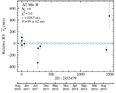
(a) AT Mic B

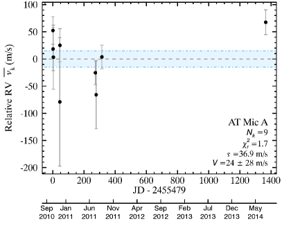
(b) AT Mic A

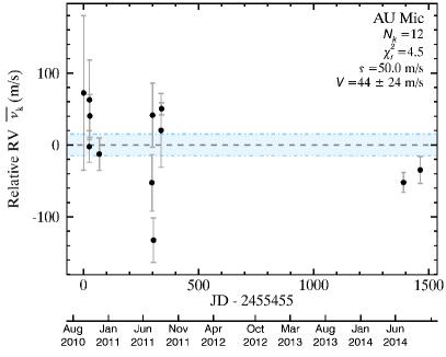
(c) AU Mic

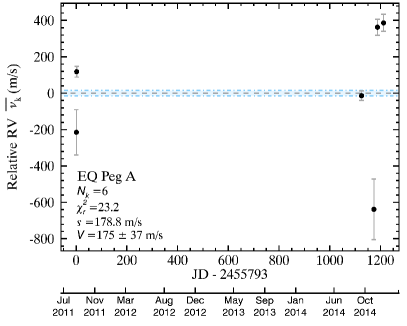
(d) EQ Peg A

Figure 2: RV curves of the targets that are present in both the young and nearby samples. The grey dashed line corresponds to the relative zero-level, whereas the light blue region delimited by dash-dotted lines corresponds to a scatter of 15 m s^-1, which is similar to the best average single-measurement precisions that we achieve. Target names are displayed in the legends as well as the total number of measurements $N_{k}$, the error-weighted reduced chi-square $\chi_{r}^{2}$ with respect to a zero-variation curve, the error-weighted standard deviation $\varsigma$ and the expected RV variability $V$ (see Section 6 for detail). See Section 7 for a discussion of the global survey results, and Section 8 for a discussion of individual targets

(a) AG Tri

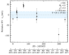
(b) $\varepsilon$ Eridani

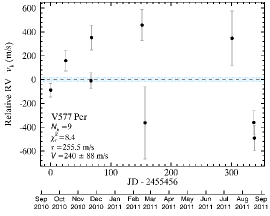
(c) V577 Per

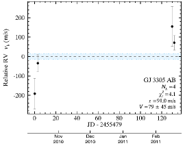
(d) GJ 3305 AB

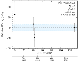
(e) TYC 5899–26–1

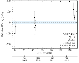
(f) V1005 Ori

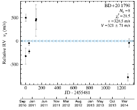
(g) BD+20 1790

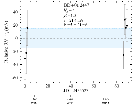
(h) BD+01 2447

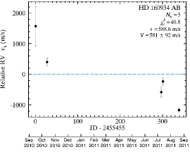
(i) HD 160934 AB

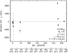
(j) LO Peg

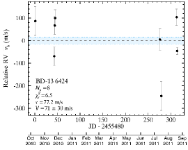
(k) BD–13 6424

Figure 3: RV curves of the young target sample. The formatting is identical to that of Figure 2. See Section 7 for a discussion of the global survey results, and Section 8 for a discussion of individual targets

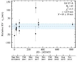
(a) GJ 15 A

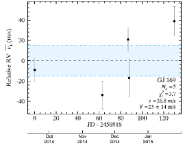
(b) GJ 169

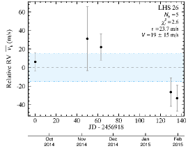
(c) LHS 26

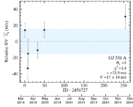
(d) GJ 338 A

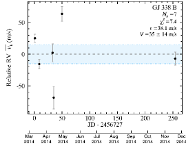
(e) GJ 338 B

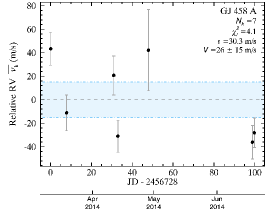
(f) GJ 458 A

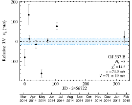
(g) GJ 537 B

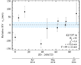
(h) GJ 537 A

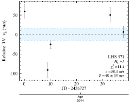
(i) LHS 371

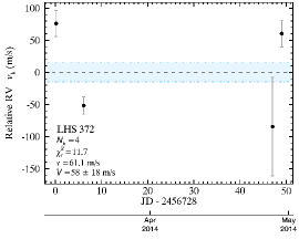
(j) LHS 372

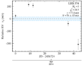
(k) LHS 374

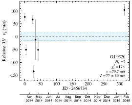
(l) GJ 9520

Figure 4: RV curves of the nearby target sample, part 1 of 2. The formatting is identical to that of Figure 2. See Section 7 for a discussion of the global survey results, and Section 8 for a discussion of individual targets

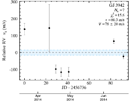
(a) GJ 3942

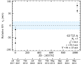
(b) GJ 725 A

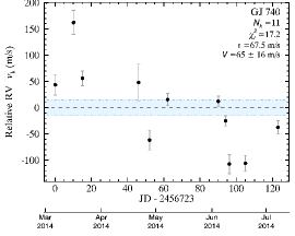
(c) GJ 740

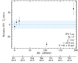
(d) EV Lac

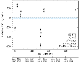
(e) GJ 876

Figure 5: RV curves of the nearby target sample, part 2 of 2. The formatting is identical to that of Figure 2. See Section 7 for a discussion of the global survey results, and Section 8 for a discussion of individual targets

Table 3: Detailed Radial Velocity Measurements

Target	Red. Julian Date			Relative
Name	JD$-2400000$			RV (m s-1)			Ratio
AG Tri	55479.003	$\pm$	0.003	107	$\pm$	51	23
	55480.930	$\pm$	0.004	-139	$\pm$	50	16
	55482.015	$\pm$	0.006	10	$\pm$	27	23
	55522.875	$\pm$	0.003	198	$\pm$	43	22
	55523.855	$\pm$	0.003	76	$\pm$	45	26
	55524.871	$\pm$	0.003	-76	$\pm$	77	20
	55608.734	$\pm$	0.004	64	$\pm$	103	22
	55611.739	$\pm$	0.003	29	$\pm$	50	25
	55759.126	$\pm$	0.004	26	$\pm$	48	20
	55793.018	$\pm$	0.004	-77	$\pm$	22	28
AT Mic A	55479.735	$\pm$	0.001	34	$\pm$	25	39
	55480.729	$\pm$	0.004	0	$\pm$	40	35
	55482.776	$\pm$	0.001	-15	$\pm$	59	28
	55523.713	$\pm$	0.001	-97	$\pm$	118	26

Note. — See Section 7 for more details.

In Table 4, we present the distributions of $\varsigma$, $\chi_{r}^{2}$, $V$, $S$ for the two survey samples. The methane gas cell and RV extraction method that we used allowed us to achieve long-term RV precisions of $S\sim$ 15–50 m s^-1, which represents an improvement of a factor $\gtrsim$ 2 over similar NIR surveys that use small observing facilities.

In Figures 6 and 7, we present the distribution of $\chi_{r}^{2}$ and $\varsigma$ as a function of the total number of epochs for all of our targets. These figures bring out the absence of a correlation between these quantities, an indication that no significant long-term systematics are affecting our survey results.

In Figure 8, we present the reduced $\chi_{r}^{2}$ with respect to zero RV variation as a function of the RV scatter $\varsigma$ for all of our targets. This figure illustrates how the young survey sample has been observed with a typically lower S/N, resulting in typical single-measurement precisions around 50 m s^-1 on average, whereas those of the nearby sample are lower at around 15 m s^-1. Targets located in the upper right of the figure (along lines of constant single-measurement precisions), are the most secure RV variables.

A Kolmogorov-Smirnov test yields a 54% probability that the reduced $\chi_{r}^{2}$ values around zero RV variation for the young and nearby samples are drawn from a single random distribution (the nearby sample targets have slightly larger $\chi_{r}^{2}$ values on average). This indicates a weak statistical significance that there is any fundamental difference in the RV variability amplitude between the two samples. We recover a larger fraction of candidate RV variable targets in the nearby sample (10/21 $\approx$ 48%) than in the young sample (4/15 $\approx$ 27%). However, considering Poisson statistics and the number of targets in each sample, there is a relatively large $\approx$ 23% chance that this discrepancy is due to pure chance. Both these results could be explained by the fact that we obtained higher S/N observations on average for the nearby sample, if we assume that there is a larger number of RV variables with an amplitude small enough so that they would not be detected in the young sample (see Figure 8).

In Figure 9, we show the RV variability $V$ as a function of the single-measurement precision $S$ and the statistical significance of $V$. The first distribution outlines the vastly different single-measurement precisions that were obtained for the young and nearby samples, which is an effect of the different S/N observations. Targets located higher up in Panel b of Figure 9 are the most probable RV variables, and those located further to the right in the same figure could correspond to more massive and/or close-in companions.

Nineteen of the targets presented in this work were never part of a precise RV follow-up ($S\lesssim$ 100 m s^-1) to date. There are, however, 13 targets that already benefitted from precise RV monitoring. These targets are listed in Table 7.2, where we compare the number of epochs, single-measurement precision and RV scatter of existing optical and NIR surveys to our survey results. For eight of the targets listed in this table, we present a more precise RV follow-up to those already published, and for five of the targets, we present the first precise RV follow-up in the NIR. There is only one case (AT Mic B) for which a NIR follow-up already existed at a better precision than the results presented here.

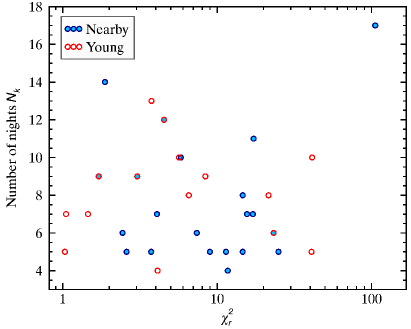
(a) Reduced chi-square value versus number of nights

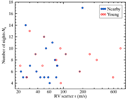
(b) RV scatter versus number of nights

Figure 6: Reduced $\chi^{2}$ with respect to zero variation and RV scatter $\sigma$ as a function of the total number of nights for which a target was observed. Young sample targets are displayed as red circles and nearby sample targets as filled blue circles. For more details, see Section 7.1.

(a) Reduced chi-square value versus $K$-band magnitude

(b) RV scatter versus $K$-band magnitude

Figure 7: Reduced $\chi^{2}$ with respect to zero variation and RV scatter $\varsigma$ as a function of the 2MASS $K_{S}$-band magnitude of our targets. The $\chi^{2}_{r}$ values do not seem to be correlated with the $K$-band magnitude, which indicates that our RV measurement errors are realistic. The RV scatter $\varsigma$ is however correlated with the $K$-band magnitude, which is a natural effect of the lower S/N that were obtained for fainter targets. The color scheme is identical to that of Figure 6. Targets in the young sample have lower S/N both because they were observed with smaller integration times as they were mostly observed before 2014, but also because they have fainter $K$-band magnitudes on average. For more details, see Section 7.1.

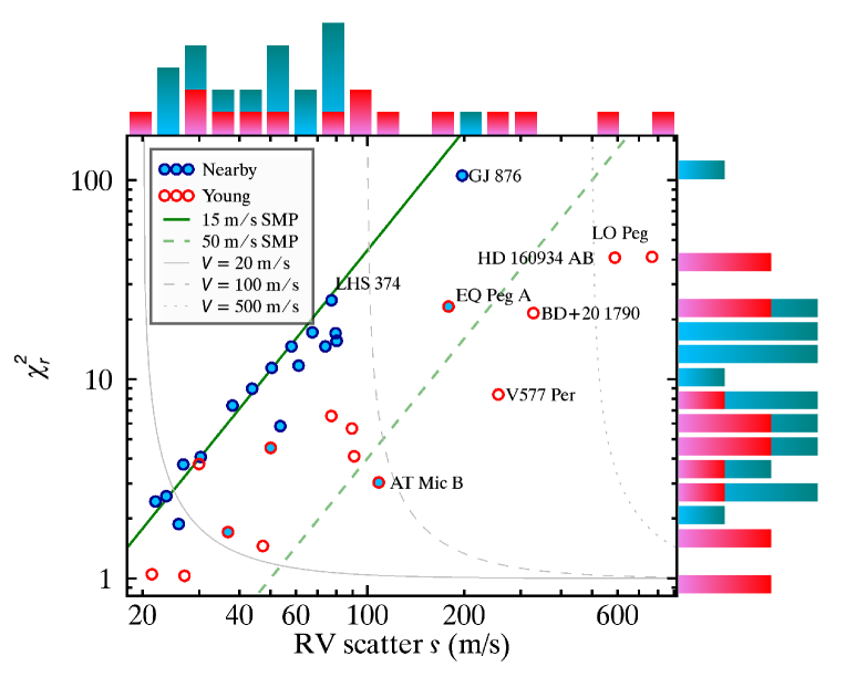
Figure 8: Reduced $\chi_{r}^{2}$ with respect to zero variation as a function of the RV scatter $\varsigma$ for targets in the nearby (filled blue circles) and young (red circles) samples. The solid and dashed green lines correspond to single-measurement precisions of 15 and 50 m s^-1, respectively. The solid, dashed and dotted grey lines correspond to respective RV variability values $V$ of 20, 100 and 500 m s^-1 ($V=\sqrt{\varsigma^{2}-S^{2}}$, see Section 6). Histogram distributions for the nearby (green bars) and young (pink bars) samples are displayed next to each plot axis. For more details, see Section 7.1.

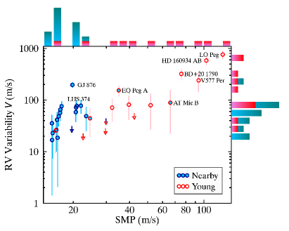
(a) RV variability versus single-measurement precision

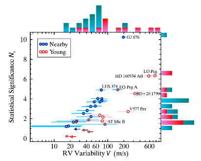
(b) Statistical significance of RV variability

Figure 9: Panel a: RV Variability $V$ as a function of single-measurement precision for the young (red circles) and nearby (blue circles) samples.
Panel b: Statistical significance as a function of the RV variability. Targets with an RV variability below 1$\sigma$ are displayed as 1$\sigma$ upper limits (left- or down-pointing arrows). For more details, see Section 7.1.

7.2 Constraints from Non-Detections

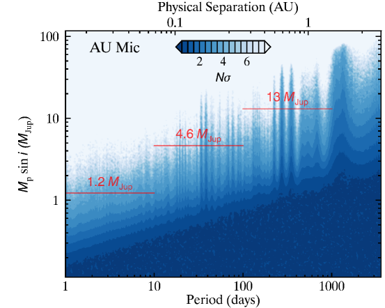
(a) AU Mic

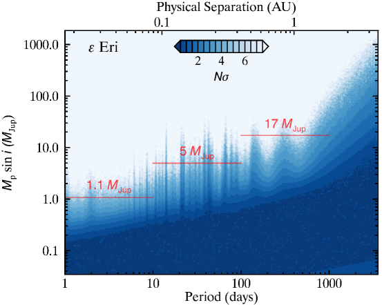
(b) $\varepsilon$ Eridani

Figure 10:

Table 4: Survey Results

Target	Survey	$N_{k}$	Baseline	Total	$\varsigma$	$\chi_{r}^{2}$	$S$	$V$	$N_{\varsigma}$	$V_{\rm max}$ (m s-1)
Name	Sample	Nights	(days)	S/N	(m s-1)		(m s-1)	(m s-1)		1$\sigma$	3$\sigma$		HJ	WJ	CJ
RV Variables
GJ 876	N	17	707	450	197	105.6	19	196	10.2	203	234		2.8	14	41
HD 160934 AB	Y	5	338	160	589	40.8	92	581	6.3	612	763		88	150	1100
LO Peg	Y	10	314	260	768	41.2	120	758	6.3	799	994		35	220	680
Candidate RV Variables
BD+20 1790	Y	8	1295	200	328	21.5	71	321	4.5	345	460		32	130	820
EQ Peg A	Y,N	5	1211	410	157	25.2	31	154	4.9	165	216		7.2	18	34
GJ 3942	N	7	92	410	80	15.6	20	78	3.8	84	118		4.1	10	300
GJ 537 B	N	8	326	500	74	14.6	19	71	3.7	78	110		3.2	5.4	45
GJ 725 A	N	5	1035	380	58	14.6	15	56	3.7	61	86		5.6	130	950
GJ 740	N	11	123	630	67	17.2	16	65	4.0	71	97		1.9	3.7	140
GJ 9520	N	7	314	460	80	17.0	19	77	4.0	84	115		4.1	11	110
LHS 371	N	5	38	400	50	11.4	15	48	3.2	53	78		3.8	8	620
LHS 372	N	4	49	270	61	11.7	18	58	3.3	64	94		8.6	41	650
LHS 374	N	5	43	410	77	24.9	15	76	4.9	81	106		6.2	12	1000
Other Targets
AG Tri	Y	10	314	240	90	5.7	38	81	2.2	94	155		3.6	16	52
AT Mic A	Y,N	9	1365	310	37	1.7	28	24	0.8	35	80		1.1	4.7	11
AT Mic B	Y,N	9	1488	320	108	3.0	62	89	1.4	111	212		2.8	13	31
AU Mic	Y,N	12	1462	480	50	4.5	24	44	1.9	52	90		1.2	4.6	13
BD+01 2447	Y	7	89	290	21	1.0	21	5	0.2	17	48		1.4	41	140
BD–13 6424	Y	8	313	260	77	6.5	30	71	2.4	81	131		4.4	30	84
$\varepsilon$ Eridani	Y	13	339	1130	30	3.8	15	26	1.7	31	56		1.1	5	17
EV Lac	N	5	193	490	44	9.0	15	41	2.8	46	70		2.5	16	36
GJ 15 A	N	14	818	490	26	1.9	19	18	0.9	25	55		0.62	2.8	8.3
GJ 3305 AB	Y	4	132	160	91	4.1	45	79	1.8	94	168		12	120	670
GJ 169	N	5	130	490	27	3.7	14	23	1.7	28	50		2.5	7.2	51
GJ 338 A	N	6	253	530	22	2.4	14	17	1.2	22	45		1.4	2	16
GJ 338 B	N	6	320	530	38	7.4	14	35	2.5	40	63		2.3	4.2	20
GJ 458 A	N	7	100	470	30	4.1	15	26	1.8	31	56		1.6	4.4	82
GJ 537 A	N	10	90	500	54	5.8	22	49	2.2	56	93		1.7	3.2	190
LHS 26	N	5	136	380	24	2.6	15	19	1.3	24	48		1.7	4.4	23
TYC 5899–26–1	Y	5	130	200	27	1.0	27	5	0.2	21	60		2.1	14	41
V1005 Ori	Y	7	131	250	47	1.5	39	26	0.7	44	105		3.6	37	120
V577 Per	Y	9	338	270	256	8.4	88	240	2.7	269	413		16	43	140

Note. — See Section 7.1 for more details on the survey results.

Table 5: Comparison With Previous Work

Target	Survey		Optical					NIR					This Work
Name	Sample		Ref.	$N_{\mathrm{data}}$	$S$ (m s-1)	$\varsigma$ (m s-1)		Ref.	$N_{\mathrm{data}}$	$S$ (m s-1)	$\varsigma$ (m s-1)		$N_{\mathrm{data}}$	$S$ (m s-1)	$\varsigma$ (m s-1)
AG Tri	Y		$\cdots$	$\cdots$	$\cdots$	$\cdots$		1	14	55	98		10	38	90
AT Mic A	Y,N		$\cdots$	$\cdots$	$\cdots$	$\cdots$		1	14	50	151		9	28	37
AT Mic B	Y,N		$\cdots$	$\cdots$	$\cdots$	$\cdots$		1	14	55	207		9	62	108
AU Mic	Y,N		$\cdots$	$\cdots$	$\cdots$	$\cdots$		1	14	50	125		12	24	50
BD+01 2447	Y		2	13	80	100		$\cdots$	$\cdots$	$\cdots$	$\cdots$		7	21	21
BD+20 1790	Y		3–5	61	5.5	580		$\cdots$	$\cdots$	$\cdots$	$\cdots$		8	71	328
$\epsilon$ Eri	Y		6	33	12.0	15.3		$\cdots$	$\cdots$	$\cdots$	$\cdots$		13	15	30
EV Lac	N		$\cdots$	$\cdots$	$\cdots$	$\cdots$		1	20	50	115		5	15	44
GJ 15 A	N		7	117	0.6	3.21		$\cdots$	$\cdots$	$\cdots$	$\cdots$		14	19	26
GJ 3305 AB	Y		8	3	20	550		1	5	50	457		4	45	91
GJ 876	N		9–13	162	2.0	162		$\cdots$	$\cdots$	$\cdots$	$\cdots$		17	19	197
GJ 725 A	N		$\cdots$	$\cdots$	$\cdots$	$\cdots$		1	18	50	51		5	15	58
V1005 Ori	Y		$\cdots$	$\cdots$	$\cdots$	$\cdots$		1	6	55	103		7	39	47

Note. — See Section 7.1 for more details.

References. — (1) Bailey et al. 2012; (2) Paulson & Yelda 2006; (3) Hernán-Obispo et al. 2015; (4) Figueira et al. 2010; (5) Hernán-Obispo et al. 2010; (6) Campbell et al. 1988; (7) Howard et al. 2014; (8) Elliott et al. 2014; (9) Rivera et al. 2010; (10) Marcy et al. 1998; (11) Marcy et al. 2001; (12) Delfosse et al. 1998a; (13) Rivera et al. 2005b.

7.3 Effects of Rotational Velocity and Age

To assess the impact of rotational broadening on our achievable RV precision limit, we have constructed a set of synthetic data based on our observations of GJ 15 A, which is a slow-rotating, RV-quiet star (within our survey precision) and benefits from a large number of high-S/N observations. We have used the best fitting parameters that were obtained from the RV pipeline for each individual raw spectrum to remove the effects of the blaze function, gas cell and telluric absorption. We have then deconvolved the remaining individual stellar spectra with the appropriate LSF and used the add_rotation.pro IDL routine to produce an artificial rotational broadening. We convolved the result with the LSF and added back the effects of the gas cell, telluric absorption and blaze function. We generated a synthetic data set in this way for 18 values of projected rotational velocities $v\sin i$ that range from 2 to 30 km s^-1.

These synthetic data sets were subsequently analyzed with the MATLAB RV pipeline as described in Section 5. We show in Figure 11(a) the resulting RV precision that was achieved as a function of projected rotational velocity. As expected, the RV precision starts decreasing when the projected rotational velocity gets larger than the velocity resolution of CSHELL ($c/R\sim 6.5$ km s^-1, where $c$ is the speed of light in vacuum). This loss of RV precision follows a power law as a function of $v\sin i$.

We have thus modelled this effect of $v\sin i$ on the RV precision by using the quadrature sum of a constant term that represents the single-measurement precision, and a two-parameters power law. The resulting fitting function is given by :

$$y=\sqrt{y_{0}^{2}+(x/\sigma_{x})^{2\beta}},$$ (15)

where $y$ is the RV precision, $x$ is the projected rotational broadening, $y_{0}$ is the RV scatter caused by all terms except rotational broadening (e.g., single-measurement precision and RV variability), and $\beta$ and $\sigma_{x}$ are the free parameters of the power-law. We find best-fit values of $\sigma_{x}=1.56\pm 0.05$ km s^-1 and $\beta=1.70\pm 0.02$. The best-fit solution is displayed as a red curve in Figure 11(a).

In Figure 11(b), we compare this relation to our survey results, assuming different single-measurement precisions. It can be noted that in several cases with relatively low projected rotational velocities ($v\sin i\lesssim 10$ km s^-1), we obtain RV precisions that do not need to include a jitter term increasing with $v\sin i$. It is however possible that a jitter term is the cause of the lower RV precision that we obtain for a few targets located above the $50$ m s^-1 single-measurement precision green solid line.

The NIR jitter–$v\sin i$ relation measured by Bailey et al. (2012) is displayed as a grey dotted line in Figure 11(b).

Such a level of jitter comparable to that of Bailey et al. (2012) is not strong enough to reproduce the RV variability of stars with known or candidate companions (GJ 876, HD 160934 AB), as well as the single stars V577 Per, BD+20 1790, and LHS 374. Those three targets display a level of RV variability that is thus unlikely to be explained by the combined loss of information due to stellar broadening and stellar jitter, however additional follow-up will be needed to assess this with certainty.

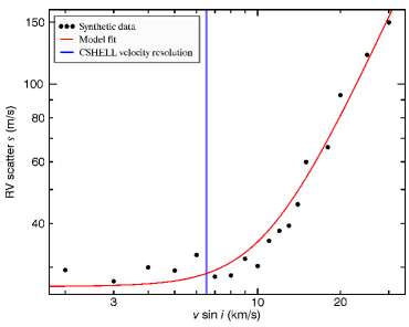
(a) Effect of $v\sin i$ on synthetic GJ 15 A RV precision

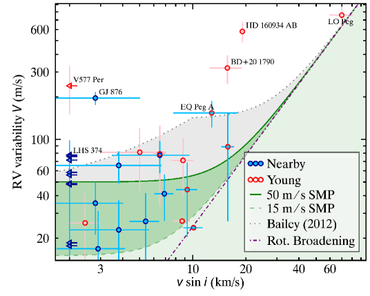
(b) RV variability and stellar jitter

Figure 11: Panel a: RV scatter $\varsigma$ as a function of the synthetic rotational velocity broadening of GJ 15 A data (black circles). The red line corresponds to a best-fit power law (see Section 7.3). The blue line corresponds to the velocity resolution of a single CSHELL spectrum ($c/R\sim 6.5$ km s^-1).
Panel b: RV variability $V$ as a function of the measured projected rotational velocity $v\sin i$ for the nearby (filled blue circles) and young (red circles) samples. Upper limits are displayed with left-pointing arrows. The purple dash-dotted line represents the effect of information loss from rotational velocity alone (extrapolated from the synthetic relation described in Section 7.3). The dashed (solid) green line represents the quadrature sum of a 15 m s^-1 (50 m s^-1) single-measurement precision and information loss from $v\sin i$. We display the quadrature sum of a 15 m s^-1 single-measurement precision with the $v\sin i$–jitter relation of Bailey et al. (2012) as a dotted grey line. It can be noted that the targets that we flag as RV variables lie outside of the NIR jitter region defined by Bailey et al. (2012), which is an indication that their RV variability might not be due to stellar activity. For more details, see Section 7.3.

Survey targets that have a larger projected rotational velocity show larger RV variations, as expected. This correlation is independent of the survey sample (i.e., independent of age), although younger stars are faster rotators on average. It can be noted that the large RV variability of LO Peg might be explained by RV information loss due to the rotational broadening of stellar lines, whereas that of EQ Peg A would require a significant jitter term at the higher end of what is admitted in the relation proposed by Bailey et al. (2012). Further observations will be required to determine whether EQ Peg A can plausibly host a substellar or planetary companion.

Figure 12:

7.4 Bi-Sector Analysis

We measured the bi-sector slopes of CO lines in each of our individual exposures (see e.g., Santos et al., 2001; Dravins, 2008) to investigate the effect of stellar activity on our RV variable targets. We did not identify a correlation between the RV and bi-sector spans in any case.

However, it must be considered that the lack of a correlation might be expected given the moderate resolution ($R\approx 46\,000$) of CSHELL . Effectively, Desort et al. (2007) noted that a poor sampling of spectral lines can hinder the measurements of bi-sector spans; e.g. a resolution of $R\approx 50\,000$ would only be able to recover bisector span variations in targets with $v\sin i\gtrsim 6$ km s^-1. observations at higher resolutions would thus be warranted to guarantee that the RV variability that we measure are not associated with stellar activity.

8 DISCUSSION OF INDIVIDUAL TARGETS

8.1 RV Variable Targets

We define targets for which we measure an RV variability with a statistical significance of $N_{\varsigma}\geq 5$ as likely RV variable, and those with $3\leq N_{\varsigma}<5$ as candidate RV variables. All targets that fall in these categories are discussed individually in this section. More follow-up observations will be needed to determine whether any RV variability is due to a companion or to stellar activity. Although it is generally expected that the impact of stellar activity is small in the near-infrared regime (Martín et al., 2006; Reiners et al., 2010), it has also been shown by Reiners et al. (2013) that under certain configurations of stellar spots and magnetic fields, the effect of jitter could in fact increase with wavelength.

GJ 876 (HIP 113020) is an M4 low-mass star (Reid et al. 1995; mass estimate 0.32 $M_{\odot}$; Rivera et al. 2005b) located at $4.69\pm 0.05$ pc (van Leeuwen, 2007). Its low rotation rate and weak magnetic activity suggest an age older than $\sim$ 0.1 Gyr. Its kinematics place it in the young disk population (Correia et al., 2010), however this does not put a strong constraint on its age (i.e., $\lesssim$ 5 Gyr, Leggett 1992).

Using the proper motion ($\mu_{\alpha}\cos\delta=959.84\pm 3.36$ $\mathrm{mas}\,\mathrm{yr}^{-1}$; $\mu_{\delta}=-675.33\pm 1.68$ $\mathrm{mas}\,\mathrm{yr}^{-1}$) and parallax measurements of van Leeuwen (2007) along with the systemic RV measurement of $-1.59\pm 0.18$ km s^-1 (Nidever et al., 2002) with the BANYAN II tool (Gagné et al., 2014; Malo et al., 2013), we obtain a significant probability ($P=85.1$%) that this system is a member of the $\beta$ Pictoris moving group, which is comparable to its other bona fide members (Gagné et al., 2014). Its $UVW$ space velocity and $XYZ$ galactic position place it at $5.05\pm 1.80$ km s^-1 and $13.3\pm 15.9$ pc from the locus of known $\beta$ Pictoris moving group members. The probability of a random interloper at such a spatial and kinematic distances from the locus of the group (counting both young and old stars) is only of $\approx$ 1.3% (Gagné et al., 2014). However, there are several indications in the literature that this system is old, e.g., Poppenhaeger et al. (2010) measured a low X-ray luminosity of $\log{L_{X}}=26.48\pm 0.13$, Rivera et al. (2005a) measured a large rotation period of $96.7$ days and a low jitter of $\sim$ 3 m s^-1, and Hosey et al. (2015) showed that it is very quiet with variation amplitudes of only $17.2$ mmag in the optical. Its absolute magnitude is about $0.7$ mag brighter than the main sequence, which could be an indication of youth, however this can be explained by its high-metallicity alone (e.g., Neves et al. 2013 measure [Fe/H] $\approx$ 0.12–40 dex). It is therefore most likely that GJ 876 is an old interloper to the $\beta$ Pictoris moving group rather than a member, as its age is not conciliable with that of the group ($24\pm 3$ Myr; Bell et al. 2015a) and a star must display both consistent kinematics and a consistent age before it can be considered as a new moving group member (Song et al., 2002; Malo et al., 2013).

Table 6: Orbital Solution for GJ 876 b

Parameter	Marcy et al. (1998)			This Paper
Orbital period $P$ (days)	$60.85$	$\pm$	$0.15$	$61.23$	$\pm$	$0.29$
Eccentricity $e$	$0.27$	$\pm$	$0.03$	$0.24$	$\pm$	$0.10$
Lon. of periastron $\omega$ (deg)	$24$	$\pm$	$6$	$209$	$\pm$	$25$
Periastron date $T_{0}$ (JD$-2.4\times 10^{6}$)	$50301.0$	$\pm$	$1.0$	$55452.7$	$\pm$	$4.6$
Planet’s mass $M_{p}\sin i$ ($M_{\mathrm{Jup}}$)	$2.11$	$\pm$	$0.20$	$2.73$	$\pm$	$0.38$
Semimajor axis $a$ (AU)	$0.21$	$\pm$	$0.01$	$0.2041$	$\pm$	$0.0007$

Note. — See Section 8.1 for more details.

Marcy et al. (1998) and Delfosse et al. (1998a) have identified a 227 m s^-1 RV signal corresponding to GJ 876 b, a Jovian planet ($M_{p}\sin i\approx 2.1$ $M_{\mathrm{Jup}}$) on an eccentric ($e=0.27\pm 0.03$) $60.85\pm 0.15$-days orbit at 0.21 AU around GJ 876. Marcy et al. (2001) subsequently discovered GJ 876 c, a $M_{p}\sin i\approx 0.6$ $M_{\mathrm{Jup}}$ planet in 2:1 resonance with GJ 876 b at 0.13 AU and on a 30.1-days orbit around GJ 876. Rivera et al. (2005b) then discovered GJ 876 d, a third, $M_{p}\sin i\approx 5.9$ $M_{\earth}$ planet on a 1.9-days orbit around GJ 876.

Correia et al. (2010) predicted the possible existence of a low-mass ($<2$ $M_{\earth}$) planet, in 4:1 orbital resonance with GJ 876 b that could explain how the high-eccentricity ($e=0.14$) of the orbit of GJ 876 d could have survived for more than $\approx$ 1 Myr, however the existence of such a planet has not been confirmed yet. Finally, Rivera et al. (2010) confirmed the existence of a fourth planet, GJ 876 e, on a 126.6-days orbit and a minimum mass of $M_{p}\sin i=12.9\pm 1.7$ $M_{\earth}$.

We followed GJ 876 as part of the nearby sample over 17 nights spanning $>$ 700 days with a typical S/N $\approx$ 170 per night, and recovered it as an RV variable target with $V=196\pm 19$ m s^-1, which is consistent within 1.6$\sigma$ with the RV amplitude measured by Marcy et al. (1998). Furthermore, we find $V_{\rm max}\big{(}N_{\varsigma}=3\big{)}=234$ m s^-1, which is also consistent with measurements in the literature.

We used the Systemic 2 software (Meschiari et al., 2009, 2012) to identify periodic signals in our RV curve that includes 17 epochs spanning $\sim$ 1.9 yr. We identified a strong signal at $P\approx 61.5$ days associated to a false alarm probability of only $3.5\cdot 10^{-4}$%. Fitting an orbital solution with the Simplex algorithm yielded orbital parameters listed in Table 6 and the orbital phase curve displayed in Figure 13. There is one data point (phase $\sim$ 313° or 2011 July 10) that is a significant outlier to this orbital fit, however it was obtained in bad weather conditions with a seeing above 3".

The period, planetary mass and eccentricity are remarkably consistent with values associated to GJ 876 b in the literature (e.g., Marcy et al., 1998), except for the argument of periastron $\omega$ that is significantly different.

Once the periodic signal of GJ 876 bc is subtracted from our data, our long-term precision does not allow us to detect any additional signal that could be associated with the other known planets orbiting GJ 876 (see Figure 13). Our analysis however demonstrates that we are able to detect planets with the characteristics of GJ 876 bc using a 3 m-class telescope and relatively inexpensive equipment.

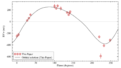
(a) Orbital Fit to GJ 876 b

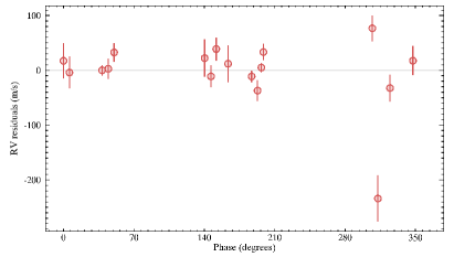
(b) Residuals for GJ 876 b

Figure 13: Panel a: Orbital fit of GJ 876 b (thick black line) to our RV measurements (red circles). We recover orbital parameters that are fully consistent with those reported in the literature. The outlier data point with a phase of $\sim$ 313° was obtained in bad weather conditions on 2011, July 10 with a seeing above 3".
Panel b: Residuals after the subtraction of GJ 876 b. Our current data does not allow us to detect the other known planetary companions to GJ 876. For more details, see Section 8.1.

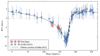
(a) Orbital Fit to HD 160934 AB

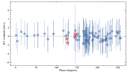
(b) Residuals for HD 160934 AB

Figure 14: Panel a: Comparison of our HD 160934 AB RV measurements (red stars) with those in the literature (blue circles) and the reported orbital solution of the system (thick black line). Our measurements are consistent with the known orbit.
Panel b: Residuals after the subtraction of the known orbit of the HD 160934 AB system. For more details, see Section 8.1.

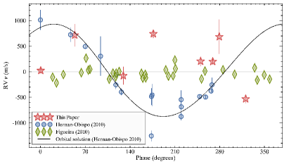
(a) Orbital Fit to BD+20 1790

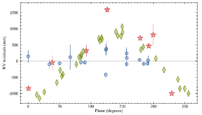
(b) Residuals for BD+20 1790

Figure 15: Panel a: Comparison of our RV measurements (red stars) with those reported by Hernán-Obispo et al. (2010; blue circles) and Figueira et al. (2010; green diamonds), as well as the suggested orbital parameters associated with the purported planet BD+20 1790 b (see Solution 1 with $e=0.05$ in Hernán-Obispo et al. 2010). We find an RV scatter that is consistent with that of Hernán-Obispo et al. (2010), suggesting that there might be an RV signal not associated with stellar activity since the amplitude does not depend on wavelength, however our data does not match the orbital solution suggested by Hernán-Obispo et al. (2010), or any of those reported in the literature for the candidate BD+20 1790 b.
Panel b: Residuals after the subtraction of the orbit suggested by Hernán-Obispo et al. (2010). For more details, see Section 8.2.

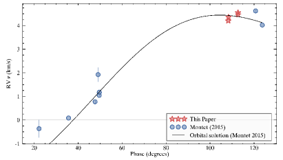
(a) Orbital Fit to GJ 3305 AB

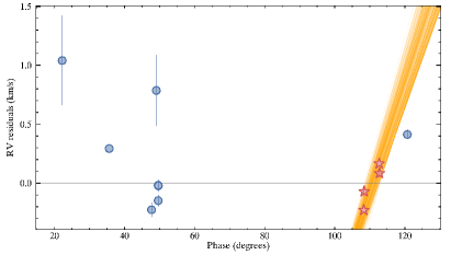
(b) Residuals for GJ 3305 AB

Figure 16: Panel a: Comparison of our RV measurements (red stars) with those reported by Montet et al. (2015) for GJ 3305 AB (blue circles) as well as their orbital solution.
Panel b: Residuals after subtracting the orbital solution of Macintosh et al. (2015). The linear trend that we measure in our RV data cannot be explained by the GJ 3305 AB orbital solution of Macintosh et al. (2015), however it remains to be determined whether it is due to an additional companion or not. For more details, see Section 8.3.

HD 160934 AB (HIP 86346) is a young and active M0-type low-mass star member of the AB Doradus moving group (Zuckerman et al., 2004; Malo et al., 2013), located at $33.1\pm 2.2$ pc (van Leeuwen, 2007). It has been confirmed as a close (0$\farcs$12) SB1 binary in an eccentric ($e\approx 0.8$), 17.1–year orbit both by the RV (Gálvez et al., 2006) and direct-imaging (Hormuth et al., 2007) methods. Its individual components have estimated spectral types of M0 and M2–M3 (Gálvez et al., 2006) and estimated masses of $0.69$ $M_{\odot}$ and $0.57$ $M_{\odot}$ (Hormuth et al., 2007).

Griffin (2013) used their RV measurements as well as those reported by López-Santiago et al. (2010), Maldonado et al. (2010) and Gizis et al. (2002) to derive an orbital solution for HD 160934 AB. They assumed an orbital inclination of $82.3\pm 0.8$ °, which was obtained from direct imaging data (Hormuth et al., 2007; Lafrenière et al., 2007; Evans et al., 2012) and stellar masses of 0.65 and 0.5 $M_{\odot}$, respectively.

We followed HD 160934 AB as part of the young sample for a total of 5 nights spanning 338 days with a typical S/N of 150 per night and recovered it as an RV variable with $V=581\pm 92$ m s^-1. We find a strong linear trend of $1853\pm 163$ m s^-1 yr^-1 in its RV curve, however the reduced $\chi_{r}^{2}$ value remains high ($11.3$) even after subtracting a linear curve.

In Figure 14, we compare our RV measurements to those reported by Griffin (2013) and we find that they are consistent with the orbital solution that they propose, however our limited time baseline only allows us to detect a linear trend in our RV data.

LO Peg (HIP 106231) is yet another young, active K8 low-mass star member of the AB Doradus moving group (Zuckerman et al., 2004; Malo et al., 2013), located at $24.80\pm 0.65$ pc (van Leeuwen, 2007). Measurements of polarization suggest the possibility that a circumstellar envelope remains around LO Peg or that significant brightness inhomogeneities exist on its surface (Pandey et al., 2009). This target has the largest rotational velocity of our sample with $v\sin i=70\pm 10$ km s^-1 (Głȩbocki & Gnaciński, 2005) and a rotation period of 0.42 days (Messina et al., 2010).

We followed LO Peg as part of the young sample for a total of 10 nights spanning 314 days with a typical S/N $\sim$ 100 and identified it as an RV variable with $V=758\pm 120$ m s^-1. The RV variability is not well fit by a linear trend and it is thus very unlikely that it can be explained by a massive stellar companion. However, it is possible that the loss of RV information due to rotational broadening of the stellar lines is the only cause of this large RV variation (see Figure 11(b)). Additional RV follow-up using a larger spectral grasp might be able to mitigate this effect.

8.2 Candidate RV Variable Targets

BD+20 1790 is a fast-rotating ($v\sin i=16\pm 3$ km s^-1; White et al. 2007), active K5-type (Reid et al., 2004) member of the AB Doradus moving group (López-Santiago et al., 2006; Malo et al., 2013), located at $38.8\pm 2.0$ pc (Shkolnik et al., 2012).

Hernán-Obispo et al. (2010) identified RV variability at an amplitude of $\approx$ 1.8 km s^-1 in the optical. Based on its photometric variability as well as analyses of its bi-sector and spectroscopic indices of chromospheric activity, they interpret the RV signal as the probable signature of a close-in (0.07 AU), massive (6–7 $M_{\mathrm{Jup}}$) planet on a 7.8–days orbit rather than the effect of chromospheric activity. They note that two solutions of different eccentricities could fit the RV data ($e=0.05\pm 0.02$ or $e=0.14\pm 0.04$).

Figueira et al. (2010) subsequently presented evidence against the interpretation of a planetary companion, by showing that the RV signal correlates with the bi-sector span of the stellar lines, and by obtaining a different RV variation amplitude of 460 m s^-1 with a periodicity of 2.8 days that correspond to the rotation period of the star.

Hernán-Obispo et al. (2015) presented a re-analysis of the RV variations of BD+20 1790 by removing the RV signal due to jitter using a Bayesian method and suggested that the RV variation is due both to stellar activity and a planetary companion. They furthermore suggest that the bisector span–RV correlation reported by Figueira et al. (2010) was due to flare events and that the correlation disappears in flare-free data. They present new orbital parameters for the candidate BD+20 1790 b that are similar to those reported by Hernán-Obispo et al. (2010), except that they find a more eccentric solution ($e\approx 0.1$ to $e\approx 0.2$).

We observed BD+20 1790 as part of the young sample for a total of 8 nights spanning $\approx$ 3.5 years with a typical S/N $\approx$ 70 per night, and recovered it as a candidate RV variable, with $V=321\pm 71$ m s^-1. Our RV curve is consistent with variations at an amplitude of $\approx$ 1 km s^-1 (see Figure 3(g)), thus providing further indication that the RV variability might not be explained by chromospheric activity alone. However, our data are inconsistent with any of the orbital solutions presented by Hernán-Obispo et al. (2010) and Hernán-Obispo et al. (2015) (e.g., see Figure 15).

Using any of our data set or those of Hernán-Obispo et al. (2010) and Figueira et al. (2010), we cannot identify a statistically significant periodicity. More follow-up observations will thus be needed to assess whether the RV variations could be caused by a companion or not. It is unlikely that the RV variability of BD+20 1790 could be explained by the loss of RV due to its fast rotation or to stellar jitter (see Figure 11(a)).

EQ Peg A (GJ 896 A; HIP 116132) is a young, M3.5-type (Newton et al., 2014; Davison et al., 2015) flaring low-mass star located at $6.58\pm 0.16$ pc (van Leeuwen, 2007). Zuckerman et al. (2013) suggested that it is a member of Octans-Near.

EQ Peg A has a stellar companion (EQ Peg B) at an angular distance of $\approx$ 5$\farcs$5 ($\approx$ 36 AU), which is an M4.0-type flare star (Davison et al., 2015).

We followed EQ Peg A as part of the young sample for a total of 6 nights spanning $\approx$ 3.3 years with a typical S/N $\approx$ 170 per night, and recovered it as a candidate RV variable with $V=175\pm 37$ m s^-1. This RV variability cannot be explained by a long-term linear trend that could be produced by EQ Peg B. The loss of RV information due to rotational broadening is not important enough to explain this large RV variability, however the addition of a jitter term at the larger end of the distribution measured by Bailey et al. (2012) could be sufficient (see Figure 11(a)). Additional follow-up will be required to address this.

GJ 3942 (HIP 79126) is a nearby M0 star (Vyssotsky, 1956) located at $16.93\pm 0.30$ pc (van Leeuwen, 2007). No precise RV measurements were reported in the literature as of yet.

We followed GJ 3942 as part of the nearby sample for a total of 7 nights spanning 92 days, at a typical S/N $\approx$ 150 per night. We identified it as a candidate RV variable with $V=78\pm 20$ m s^-1. A high-S/N follow-up over a longer baseline will be useful to determine whether this RV signal is physical or not.

GJ 537 B (HIP 68588 B) is a nearby M0 star (Gaidos et al., 2014) located at $12.3\pm 0.9$ pc (Jenkins, 1952). It is a companion to GJ 537 A at an angular separation of $\approx$ 2$\farcs$9.

We followed GJ 537 B as part of the nearby sample for a total of 8 nights spanning a total of 326 days with a typical S/N $\approx$ 180 per night. We recovered it as a candidate RV variable with $V=71\pm 19$ m s^-1. Additional follow-up measurements will be needed to determine the nature of this likely RV variability.

GJ 725 A (HIP 91768) is a nearby ($3.57\pm 0.03$ pc; van Leeuwen 2007), quiet and slowly-rotating M3-type star (Jenkins et al., 2009).

Nidever et al. (2002) have shown that GJ 725 A is stable within 100 m s^-1 on a baseline of $\approx$ 3 years and Endl et al. (2006) further constrained its RV stability by obtaining a scatter of only 7.4 m s^-1 in their RV measurements over a baseline of $\approx$ 7 years.

GJ 725 A has a co-moving M3.5-type (Jenkins et al., 2009) companion (GJ 725 B; HIP 91772) at an angular separation of $\approx$ 13$\farcs$3. Endl et al. (2006) report that they detect a linear RV slope of $6.99\pm 0.86$ m s^-1 yr^-1 in the GJ 725 A data over a 7.09 year baseline, which they interpret as a small portion of its orbit around the center of mass of GJ 725 AB.

We followed GJ 725 A as part of the nearby sample for a total of 5 nights that spanned 2.8 years with a typical S/N $\approx$ 170 per night and identified it as a candidate RV variable with $V=56\pm 15$ m s^-1. Our data is be well fit by a linear trend with a slope of $35\pm 5$ m s^-1 yr^-1,

Using the projected separation of GJ 725 AB ($\approx$ 47 AU) and assuming typical masses of $\approx$ 0.36 $M_{\odot}$ and $\approx$ 0.3 $M_{\odot}$ that correspond to their respective spectral types of M3 and M3.5 (Reid & Hawley, 2005; Kaltenegger & Traub, 2009), their orbital period should be $P\approx 400$ years. This corresponds to a tangential velocity of $v\approx 1.75$ km s^-1 as measured from the center of mass in the case of a circular orbit. In the extreme case where the orbit is seen edge on from the Earth, we could expect a change of RV of up to $\approx$ 25 m s^-1 yr^-1 per year. Our RV slope measurement is slightly larger than this, which could be an indication that the orbit of GJ 725 AB is eccentric (e.g., $e\gtrsim 0.155$ would be sufficient).

We thus measure an RV slope that is consistent with the orbit of GJ 725 AB as long as it is slightly eccentric, however in the $\approx$ 9 years that separate our measurements from those of Endl et al. (2006), it might seem surprising that the RV slope has changed by $\approx$ 28 m s^-1 yr^-1. Assuming that both our measurements are consistent with the orbit of GJ 725 AB indeed puts a much stronger constraint on its eccentricity, at $e\gtrsim 0.435$.

GJ 740 (HIP 93101) is a nearby, weakly active M0.5 star (Reiners et al., 2012) located at $10.91\pm 0.18$ pc (van Leeuwen, 2007). No precise RV measurements were reported in the literature as of yet.

We followed GJ 740 as part of the nearby sample for a total of 11 nights spanning 123 days with a typical S/N $\approx$ 190 per night. We recovered it as a candidate RV variable with $V=65\pm 16$ m s^-1. A high-S/N follow-up over a longer baseline will be useful to determine whether this RV signal is physical or not. We note a significant linear trend in our RV curve with a slope of $-415\pm 44$ m s^-1 yr^-1, however we obtain a high reduced $\chi_{r}^{2}$ value of $\approx$ 10.2 from a linear fit, which indicates that the scatter is still relatively high even when the linear trend is subtracted. We obtain $\varsigma=46.3$ m s^-1 and $V=43.4\pm 16.3$ m s^-1 ($N_{\varsigma}=2.7$) after the subtraction, which would not qualify for an additional statistically significant variation under our criteria.

GJ 9520 (HIP 75187) is a nearby M1.5-type (Reid et al., 2004) star located at $11.41\pm 0.24$ pc (van Leeuwen, 2007). No precise RV measurements were reported in the literature for this star as of yet.

We followed GJ 9520 as part of the nearby sample for a total of 7 nights spanning 314 days with a typical S/N $\approx$ 170 per night. We recovered it as a candidate RV variable with $V=77\pm 19$ m s^-1. Additional follow-up will be needed to determine whether this RV signal is physical or not.

LHS 371 (HIP 70529) and LHS 372 (HIP 70536) form a binary stellar system located at $16.36\pm 0.40$ pc (van Leeuwen, 2007) with respective spectral types of M0 and M1 (Gaidos et al., 2014), and are separated by $\approx$ 45". No precise RV measurements for any of the two components were reported in the literature as of yet.

We followed both LHS 371 and LHS 372 as part of the nearby sample for a total of 5 and 4 nights that span 38 and 49 days with typical S/N precisions of $\approx$ 180 and 135 per night, respectively. Both components were identified as candidate RV variables, with $V=48\pm 15$ m s^-1 (LHS 371) and $V=58\pm 18$ m s^-1 (LHS 372). Subsequent follow-up will be needed to determine whether this RV variation is physical.

LHS 374 (HIP 70956) is a slow rotating and chromospherically inactive, nearby M0 star (Gaidos et al., 2014) located at $16.99\pm 0.42$ pc (van Leeuwen, 2007). No precise RV measurements were reported in the literature for this star as of yet.

We followed LHS 374 as part of the nearby sample for a total of 5 nights spanning 43 days with a typical S/N $\approx$ 180 and recovered it as a candidate RV variable with $V=76\pm 15$ m s^-1. Subsequent follow-up will be needed to determine whether this RV variation is physical.

8.3 Likely Linear Trends in RV Curves

The presence of a massive companion at a large enough separation can induce a linear variation in our RV curves with a period that possibly exceeds our temporal baseline coverage of a given target. The criteria defined above, which are based on the scatter of RV points around the mean, will be less sensitive to detecting such variations in a given RV curve, compared with one where at least one period is sufficiently sampled. In order to identify such candidate RV variables, we have fit a linear slope to all RV curves presented in this work using the IDL routine mpfitfun.pro written by Craig B. Markwardt. In this section, we focus on the targets for which a linear fit yielded a reduced chi-square of at most 3, corresponding to an non-null RV slope at a statistical significance of at least 3$\sigma$. These criteria have yielded 3 likely RV variable targets :

GJ 458 A is a nearby M0 star (Reid et al., 2004) located at $15.52\pm 0.34$ pc (van Leeuwen, 2007). It has an M3-type companion (GJ 458 B, or BD+55 1519 B; Hawley et al. 1997) at an angular distance of $\approx$ 14$\farcs$7.

We followed GJ 458 A as part of the nearby sample for a total of 7 nights spanning 100 days with a typical S/N $\approx$ 180 per night. We did not recover it as a statistically significant RV variable in terms of RV scatter on our total baseline, however its RV curve is well fit by a linear trend ($\chi_{r}^{2}=3.0$) with a corresponding slope of $-185\pm 50$ m s^-1 yr^-1 (3.7$\sigma$ significance; see Figure 4(f)).

Assuming a mass of $\approx$ 0.58 $M_{\odot}$ for GJ 458 A (Gaidos et al., 2014) and a mass of $\approx$ 0.36 $M_{\odot}$ for GJ 458 B that is typical of a field M3 star (Reid & Hawley, 2005; Kaltenegger & Traub, 2009) and using the projected separation of $\approx$ 228 AU, we would expect a period of $\approx$ 3550 years for the orbit of the GJ 458 AB system in a case with zero eccentricity. This would be consistent with a maximal RV slope of only $\approx$ 1.2m s^-1 yr^-1. Only an well-aligned extremely eccentric orbit ($e\gtrsim 0.95$) could explain this, which is highly unlikely. It is thus probable that we are not measuring the effect of GJ 458 B, but rather possibly that of an unknown, massive companion. It is unlikely that this RV signal is due to stellar jitter, as this would yield a more rapidly varying random RV signal, and GJ 458 A is an inactive, slow-rotating star (Herrero et al., 2012).

GJ 3305 AB is a known 0$\farcs$093 binary low-mass M0-type (Kasper et al., 2007) member of the $\beta$ Pictoris moving group located at $29.8\pm 0.8$ pc. It has been identified as a 66" common proper motion companion system to the F0-type star 51 Eridani (Feigelson et al., 2006), which itself has a 2 $M_{\mathrm{Jup}}$ planetary, T-type companion identified by the method of direct imaging (Macintosh et al., 2015). This system will thus be a very important benchmark to understand stellar and planetary properties at young ages in the near future.

Montet et al. (2015) recently led a full RV and astrometric characterization of the GJ 3305 AB pair and their orbital properties. They found a period of $29.16\pm 0.65$ yr, a semi-major axis of $9.8\pm 0.15$ AU, an eccentricity of $0.19\pm 0.02$ and individual masses of $0.65\pm 0.05$ and $0.44\pm 0.05$ $M_{\odot}$ for A and B, respectively. They compared the observed dynamical masses with evolutionary models to derive an age of $28^{+15}_{-6}$ Myr for the system, consistent with the age of the $\beta$ Pictoris moving group ($24\pm 3$ Myr; Bell et al. 2015a). They, however, obtain a dynamical mass for GJ 3305 B that is discrepant with that of evolutionary models, which they suggest could be explained by the presence of an unresolved companion.

Delorme et al. (2012) have identified a potential 0$\farcs$38 companion to GJ 3305 A by direct imaging in a 2009 NACO image in the $L^{\prime}$ band, however further observations obtained in 2012 revealed that it was not a planetary companion, but rather a speckle or a background star.

We observed the unresolved GJ 3305 AB pair during a total of 4 nights at a typical S/N$\approx 80$ per night over a period of 5 months as part of the young sample. The RV curve of this target is well fit by a linear trend ($\chi_{r}^{2}=1.8$) with a corresponding slope of $435\pm 145$ m s^-1 yr^-1 (3.0$\sigma$ significance; Figure 3(d)).

In Figure 16, we compare our measurements with those reported by Montet et al. (2015) and find that our observed linear trend is inconsistent with the orbital solution that they suggest. More follow-up data will be needed to confirm whether there is an additional RV variability to this system that is statistically significant.

8.4 Other Noteworthy Targets

We describe in this section the targets that we did not select as candidate RV variables, but for which relevant information is available in the literature.

GJ 15 A: Howard et al. (2014) reported the detection of a $5.35$ $M_{\oplus}$ planet in a $11.443$-day orbit around GJ 15 A. Our data lack the precision and cadence necessary to detect the planet outright. However, by assuming the planet period and ephemeris reported by Howard et al. (2014), we can place a constraint on the mass of the planet with the data presented here. We used our 10 per-night RV measurements with uncertainties of $<60$ m s^-1, and phased them an $11.443$-day period and ephemeris reported by Howard et al. (2014). We averaged measurements between phases of 0–$\pi$ $\mathrm{rad}$, and subsequently between $\pi$–$2\pi$ $\mathrm{rad}$. We then subtracted the results obtained from these two averages and converted this number into a semi-amplitude by making use of the fact that a similar operation carried out on a sinusoidal wave (i.e., subtracting its average between phases of 0–0.5 $\mathrm{rad}$ and that between 0.5–1 $\mathrm{rad}$) is equal to $\sqrt{3}\,K$, where $K$ is its semi-amplitude. We used the approximation that our RV measurements are evenly distributed in phase to derive $K=8$ m s^-1. In order to quantify the uncertainty on this measurement, we computed a Monte Carlo simulation of 20 trial periods. For each trial period, we carried out the same phase-averaged measurement of the semi-amplitude, and measured a standard deviation of 12 m s^-1. We thus derive a value of $K=8\pm 12$ m s^-1 for the RV variation semi-amplitude of GJ 15 A, which corresponds to a 3$\sigma$ upper limit of $<36$ m s^-1 on its RV variation, or an upper limit of $<66$ $M_{\oplus}$ on the mass of its companion.

$\varepsilon$ Eridani is a young K2 star located at $3.216\pm 0.002$ pc (van Leeuwen, 2007), for which disputed planet candidates have been reported by Campbell et al. (1988) and Quillen & Thorndike (2002), associated with RV scatters lower than 15 m s^-1.

We followed this target as part of the young survey for a total of 13 nights spanning 339 days, with a typical S/N $\approx$ 300 per night. We did not identify it as an RV variable ($V=26\pm 15$ m s^-1), however we lack the long-term precision that would be needed to determine whether the signal reported by Campbell et al. (1988) are spurious.

9 CONCLUSION

In this paper we report the results of a precise NIR RV survey of 32 low-mass stars with spectral types K2–M4, carried out with CSHELL and an isotopologue gas cell at the NASA IRTF, 19 of which were never followed by high precision RV surveys. We used a novel data reduction and RV extraction pipeline to demonstrate that we can achieve short-term photon-limited RV precisions of $\approx$ 8 m s^-1 with long-term stability of $\approx$ 15 m s^-1, which are unprecedented using a small telescope that is easily accessible to the community.

We used the non-detections of our survey to assign upper limits on the masses of close-in companions to our targets, and we provide the first multi-wavelength confirmation of GJ 876 bc and recover orbital parameters that are fully consistent with those reported in the literature. We obtained RV curves for two binary systems (HD 160934 AB, GJ 725 AB) that are consistent with the literature, and report that GJ 740 and GJ 458 A could be bound to unknown, long-period and massive companions. We identified 7 new candidate RV variables (EQ Peg A, GJ 3942, GJ 537 B, GJ 9520, LHS 371, LHS 372, and LHS 374) with statistical significances in the 3–5$\sigma$ range. Additional observations will be needed to verify whether these RV variable stars host substellar or planetary companions.

Comparing our results with the projected rotational velocities of our sample, we showed that the proposed jitter relation of Bailey et al. (2012) is not large enough to account for the observed RV variations of LHS 374, BD+20 1790 and V577 Per. The probability that targets in the nearby sample display larger RV variations than those in the young sample is of 54%; the two samples are thus not significantly different in this regard. We find that very active stars in our survey can display RV variabilities down to $\sim$ 25–50 m s^-1, providing a constraint on the effect of jitter in the NIR.

In the near future, iSHELL will be mounted on the IRTF with a methane gas cell similar to that used in this work; the improved spectral grasp ($\approx$ 50 times larger), resolution ($R\approx 70\,000$) and instrumental sensitivity will achieve RV precisions of $\lesssim$ 5 m s^-1 that will allow the detection of super-Earth planets ($\gtrsim$ 13 $M_{\earth}$) near the habitable zone of mid-M low-mass stars in the solar neighborhood. Achieving such precisions on active, very low-mass stars using optical facilities will be challenging, hence NIR RV techniques will play a key role in characterizing Earth-like planets in the habitable zone of low-mass stars. These will serve as a crucial complement to transiting exoplanet studies, as the combination of both the RV and transit methods will provide a measurement of the mean planet density and put strong constraints on the physical properties of future Earth-like discoveries.

References

- Akeson et al. (2013) Akeson, R. L., Chen, X., Ciardi, D., et al. 2013, Publications of the Astronomical Society of the Pacific, 125, 989
- Anglada-Escudé et al. (2012) Anglada-Escudé, G., Plavchan, P., Mills, S., et al. 2012, Publications of the Astronomical Society of the Pacific, 124, 586
- Arfken et al. (2012) Arfken, G. B., Weber, H.-J., & Harris, F. E. 2012, Mathematical Methods for Physicists, A Comprehensive Guide (Academic Press)
- Arriagada (2011) Arriagada, P. 2011, The Astrophysical Journal, 734, 70
- Bailey et al. (2012) Bailey, J. I. I., White, R. J., Blake, C. H., et al. 2012, The Astrophysical Journal, 749, 16
- Bean et al. (2010) Bean, J. L., Seifahrt, A., Hartman, H., et al. 2010, The Astrophysical Journal, 713, 410
- Bell et al. (2015a) Bell, C. P. M., Mamajek, E. E., & Naylor, T. 2015a, arXiv.org, 5955
- Bell et al. (2015b) —. 2015b, Monthly Notices of the Royal Astronomical Society, 454, 593
- Blake et al. (2010) Blake, C. H., Charbonneau, D., & White, R. J. 2010, The Astrophysical Journal, 723, 684
- Blake & Shaw (2011) Blake, C. H., & Shaw, M. M. 2011, Publications of the Astronomical Society of the Pacific, 123, 1302
- Bonfils et al. (2013) Bonfils, X., Delfosse, X., Udry, S., et al. 2013, A&A, 549, 109
- Bottom et al. (2013) Bottom, M., Muirhead, P. S., Johnson, J. A., & Blake, C. H. 2013, Publications of the Astronomical Society of the Pacific, 125, 240
- Browning et al. (2010) Browning, M. K., Basri, G., Marcy, G. W., West, A. A., & Zhang, J. 2010, The Astronomical Journal, 139, 504
- Butler et al. (2004) Butler, R. P., Vogt, S. S., Marcy, G. W., et al. 2004, The Astrophysical Journal, 617, 580
- Butler et al. (2006) Butler, R. P., Wright, J. T., Marcy, G. W., et al. 2006, The Astrophysical Journal, 646, 505
- Campbell et al. (1988) Campbell, B., Walker, G. A. H., & Yang, S. 1988, Astrophysical Journal, 331, 902
- Cochran & Hatzes (1994) Cochran, W. D., & Hatzes, A. P. 1994, Astrophysics and Space Science, 212, 281
- Cochran et al. (2002) Cochran, W. D., Hatzes, A. P., Endl, M., et al. 2002, American Astronomical Society, 34, 916
- Correia et al. (2010) Correia, A. C. M., Couetdic, J., Laskar, J., et al. 2010, Astronomy & Astrophysics, 511, A21
- Crockett et al. (2011) Crockett, C. J., Mahmud, N. I., Prato, L., et al. 2011, The Astrophysical Journal, 735, 78
- Cutispoto et al. (2000) Cutispoto, G., Pastori, L., Guerrero, A., et al. 2000, Astronomy & Astrophysics, 364, 205
- Davison et al. (2015) Davison, C. L., White, R. J., Henry, T. J., et al. 2015, The Astronomical Journal, 149, 106
- Delfosse et al. (1998a) Delfosse, X., Forveille, T., Mayor, M., et al. 1998a, Astronomy & Astrophysics, 338, L67
- Delfosse et al. (1998b) Delfosse, X., Forveille, T., Perrier, C., & Mayor, M. 1998b, Astronomy & Astrophysics, 331, 581
- Delorme et al. (2012) Delorme, P., Lagrange, A.-M., Chauvin, G., et al. 2012, Astronomy & Astrophysics, 539, A72
- Desort et al. (2007) Desort, M., Lagrange, A.-M., Galland, F., Udry, S., & Mayor, M. 2007, Astronomy & Astrophysics, 473, 983
- Dravins (2008) Dravins, D. 2008, Astronomy & Astrophysics, 492, 199
- Dumusque et al. (2012) Dumusque, X., Pepe, F., Lovis, C., et al. 2012, Nature, 491, 207
- Duncan et al. (1991) Duncan, D. K., Vaughan, A. H., Wilson, O. C., et al. 1991, Astrophysical Journal Supplement Series (ISSN 0067-0049), 76, 383
- Eiroa et al. (2013) Eiroa, C., Marshall, J. P., Mora, A., et al. 2013, Astronomy & Astrophysics, 555, A11
- Elliott et al. (2014) Elliott, P., Bayo, A., Melo, C. H. F., et al. 2014, Astronomy & Astrophysics, 568, A26
- Endl et al. (2006) Endl, M., Cochran, W. D., Kürster, M., et al. 2006, The Astrophysical Journal, 649, 436
- Endl et al. (2003) Endl, M., Cochran, W. D., Tull, R. G., & MacQueen, P. J. 2003, The Astronomical Journal, 126, 3099
- Evans et al. (2012) Evans, T. M., Ireland, M. J., Kraus, A. L., et al. 2012, The Astrophysical Journal, 744, 120
- Fabricius et al. (2002) Fabricius, C., Høg, E., Makarov, V. V., et al. 2002, A&A, 384, 180
- Feigelson et al. (2006) Feigelson, E. D., Lawson, W. A., Stark, M., Townsley, L., & Garmire, G. P. 2006, The Astronomical Journal, 131, 1730
- Figueira et al. (2010) Figueira, P., Marmier, M., Bonfils, X., et al. 2010, Astronomy & Astrophysics, 513, L8
- Gagné et al. (2014) Gagné, J., Lafrenière, D., Doyon, R., Malo, L., & Artigau, É. 2014, The Astrophysical Journal, 783, 121
- Gaidos et al. (2014) Gaidos, E., Mann, A. W., Lépine, S., et al. 2014, Monthly Notices of the Royal Astronomical Society, 443, 2561
- Gálvez et al. (2006) Gálvez, M. C., Montes, D., Fernández-Figueroa, M. J., & López-Santiago, J. 2006, Astrophysics and Space Science, 304, 59
- Gizis et al. (2002) Gizis, J. E., Reid, I. N., & Hawley, S. L. 2002, The Astronomical Journal, 123, 3356
- Głȩbocki & Gnaciński (2005) Głȩbocki, R., & Gnaciński, P. 2005, in Proceedings of the 13th Cambridge Workshop on Cool Stars, 571
- Gray et al. (2003) Gray, R. O., Corbally, C. J., Garrison, R. F., McFadden, M. T., & Robinson, P. E. 2003, The Astronomical Journal, 126, 2048
- Greene et al. (1993) Greene, T. P., Tokunaga, A. T., Toomey, D. W., & Carr, J. B. 1993, Proc. SPIE Vol. 1946, 1946, 313
- Griffin (2013) Griffin, R. F. 2013, The Observatory, 133, 322
- Hawley et al. (1997) Hawley, S. L., Gizis, J. E., & Reid, N. I. 1997, Astronomical Journal v.113, 113, 1458
- Henry et al. (2014) Henry, T. J., Jao, W.-C., Pewett, T., et al. 2014, American Astronomical Society, 224
- Henry et al. (2006) Henry, T. J., Jao, W.-C., Subasavage, J. P., et al. 2006, The Astronomical Journal, 132, 2360