The LOFAR Solar Imaging Pipeline and the LOFAR Solar Data Center

Abstract

LOFAR is a new and sensitive radio interferometer that can be used for dynamic high-resolution imaging spectroscopy at low radio frequencies from 10 to 90 and 110 to 250 MHz. Here we describe its usage for observations of the Sun and in particular of solar radio bursts. We also describe the processing, archiving and accessing of solar LOFAR data, which is accomplished via the LOFAR Solar Imaging Pipeline and the LOFAR Solar Data Center.

1 Introduction

The Sun is a low to moderate activity star and because of its proximity to Earth a unique astrophysical object for studying stellar phenomena in great detail. Radio observations can make substantial contributions to such studies since the Sun is an intense radio source. Its $10^{6}$ K hot corona emits thermal radio radiation. In addition, solar activity produces intense non-thermal radio radiation observed as radio bursts [McLean, 1985, Warmuth & Mann, 2005, Mann, 2006]. They are caused by a release of energy during a reconfiguration of the Sun’s magnetic field which also results in flares and eruptive events such as coronal mass ejections. The radiation is generated by plasma emission and emitted near the local plasma frequency and/or its harmonics [Melrose, 1985]. For instance, type III bursts are a typical phenomenon in solar radio radiation and are signatures of energetic electrons propagating along magnetic field lines in the corona [Wild, 1950, Suzuki & Dulk, 1985, Breitling et al., 2011]. Since the radio emission occurs near the local electron plasma frequency $f_{\mathrm{pe}}=(e^{2}N_{\mathrm{e}}/\epsilon_{0}m_{\mathrm{e}})^{1/2}/2\pi$ ($e$, elementary charge; $\epsilon_{0}$, permittivity of free space; $m_{\mathrm{e}}$, electron mass), and because of the gravitational density stratification of the corona, higher and lower frequencies are emitted in the lower and higher corona, respectively.

With the Low Frequency Array (LOFAR, van Haarlem et al. [2013]) a sensitive high resolution radio interferometer became available for radio observations in the frequency range from 10 to 250 MHz corresponding to a radial distance between 1 and 3 solar radii ($R_{\odot}$) in the corona [Mann et al., 1999]. Its capability for high resolution dynamic imaging spectroscopy makes it particularly useful for spatial and time resolved observations of solar radio burst. The LOFAR Key Science Project “Solar Physics and Space Weather with LOFAR” (Solar KSP, Mann et al. [2011]) was formed to use LOFAR for solar observations and to address open questions. Its goals are the coordination of solar observations, the solar data processing and analysis and the provision of the resulting data products to the scientific community. These goals led to the development of the LOFAR Solar Imaging Pipeline and the LOFAR Solar Data Center described here.

2 LOFAR

LOFAR [van Haarlem et al., 2013] is a European digital radio interferometer developed under the leadership of the Netherlands Institute for Radio Astronomy (ASTRON). It currently consists of 48 antenna stations distributed over the Netherlands (40), Germany (5), United Kingdom (1), France (1) and Sweden (1) with its center near Netherlands city Groningen. Additional stations are currently under constructions in Poland (3) and Germany (1) or in the planning phase. A LOFAR station consists of high- and low-band antenna fields and an electronics container with the receiver and computer hardware. An antenna field is composed of identical antennas, which are added to a station beam (or pointing) to receive the signal from a specific sky direction. The data of the station pointings are sent to the correlator in Groningen which forms the array or sub-array pointings.

LOFAR operates in the low frequency range from $10-90$ (low-band) and $110-250$ MHz (high-band) in full polarization with high sensitivity and resolution for imaging spectroscopy. LOFAR’s beam forming allows for the simultaneous observation of several different sky regions, which is important for the calibration of highly variable radio sources like the Sun. It also allows the simultaneous recording of dynamic radio spectra and images at different frequencies. These capabilities make LOFAR a very powerful instrument for imaging spectroscopy of celestial radio sources and to a radio heliograph if applied to the Sun.

3 The Solar Imaging Pipeline

The Solar Imaging Pipeline is a software package for analyzing LOFAR observations of the Sun. It was developed by the Solar KSP at the Leibniz-Institut für Astrophysik Potsdam (AIP) as an extension of the LOFAR Standard Imaging Pipeline [Heald et al., 2011] to accomplish a proper data processing for solar LOFAR data. It is necessary because of the differences between solar and standard observations and the consequences for the data processing. They are summarized in Table 2 and 2 and explained below.

Table 1: Differences between observations of the Sun and standard radio sources.

	Standard radio source	Sun
Temporal resolution [s]	$\geq 10^{4}$	$\leq 1$
Spatial resolution [arcsec]	$\sim 1$	$\sim 10^{1}$
No. of stations	$\geq 48$	$\leq 30$
No. of baselines	$>10^{3}$	$<5\times 10^{2}$
Field of view [deg]	$>10^{1}$	$\sim 1$
Typical flux density [Jy]	$\ll 10^{3}$	$10^{4}-10^{12}$
Typical noise level [Jy]	$10^{-1}$	$10^{2}$
Dynamic range of flux density [orders of magnitude]	0	8
Ionospheric scintillation	low	high
High res. dynamic spectroscopy	no	yes

Table 2: Differences between standard and solar data processing resulting from the differences in the observations of Table 2.

	Standard Imaging	Solar Imaging
Aperture synthesis	yes	no
Flagging	in frequency & time	in frequency only
uv-range [wavelengths]	$0-10^{6}$	$0-10^{3}$
Sky model source threshold	$\leq 50$ Jy	$\sim 10^{3}$ Jy
Distance calibrator - target	$\leq 1$ deg	$\geq 5$ deg
Demixing	yes	no
Imager	AWImager	CASA imager
CLEAN algorithms	Clark for point sources	multi-scale for ext. sources
Self-calibration	yes	limited to selected events
Solar Data Center	no	yes

3.1 Characteristics of solar observations

3.1.1 High variability of solar radio emission

The radio emission from most radio sources that LOFAR observes such as galaxies is constant and ranges from 0.1 to 100 Jy. However, the emission from the Sun at 100 MHz is about $10^{4}$ Jy (1 solar flux unit, sfu) during quiet periods but it can rise to $10^{12}$ Jy ($10^{8}$ sfu) within a few seconds in case of solar radio bursts [Mann, 2010, Dulk, 2000] which can occur anywhere near the Sun. So solar radio observations need to be able to record a dynamic range in brightness of 8 orders of magnitude with a time resolution of seconds. Consequences:

• A time resolution of seconds prevents the typical aperture synthesis which uses the Earth’s rotation and observation times of hours for increasing the uv-coverage and image quality. Fig. 1 and 2 show the uv-coverage with and without aperture synthesis for comparison. Each point in the uv-plane represent a baseline.

• The short duration of some bursts prevents temporal radio frequency interference (RFI) removal also called flagging, since flagging of radio peaks could also remove the signals of solar bursts.

• Dynamic radio spectra are recorded simultaneously with the imaging data, since they can provide a higher time and frequency resolution at a lower data rate. They also support the identification of solar bursts in LOFAR data.

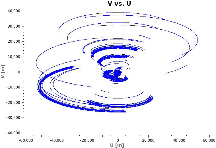
Figure 1: uv-coverage (baselines) for 12 hours of data. Because of the Earth’s rotation each point in the uv-plane multiplies into an arc like point set.

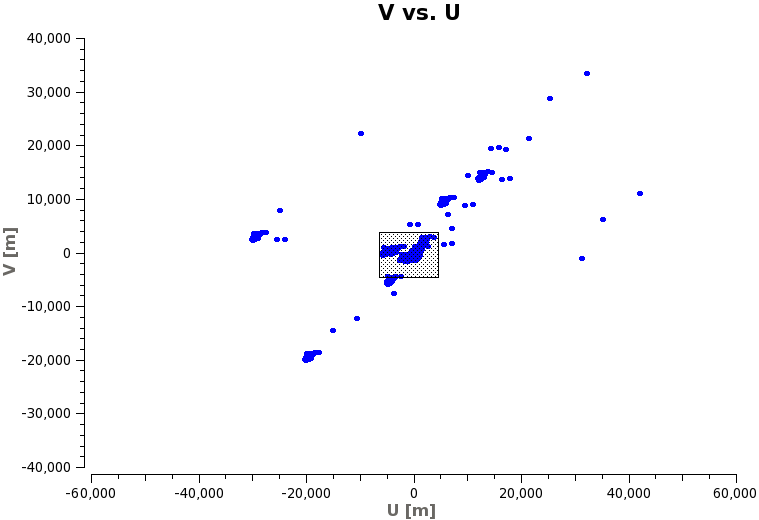
Figure 2: uv-coverage for 1 second of data. The box indicates the approximate region of points (baselines) that remain if the uv-range is limited to $\leq 1000$ wavelengths.

3.1.2 Limited resolution in the corona

While standard targets can be resolved with sub-arcsec resolution, the spatial resolution of solar observations is limited to a few ten arcsec by turbulence in the corona [Bastian, 2004]. Consequences:

• Since the angular resolution is proportional to the inverse of the baseline length, the uv-range can be limited to a maximum baseline length of 1000 wavelengths. The box in Fig. 2 marks the approximate subset of stations that remains with this limitation.

• International stations and some remote stations are not needed since they provide only baselines with a length of more than 1000 wavelengths. This reduces the number of baselines $n_{b}=n_{s}\times(n_{s}-1)/2$ (where $n_{s}$ is the number of stations) and therefore limits the image resolution.

3.1.3 Sufficient field of view

Since solar radio emission is a result of plasma emission determined by the plasma density of the corona, radio emission in the frequency range from 10 to 240 MHz is limited to a region within 3$R_{\odot}$. This region is well contained with the LOFAR field of view of approximately 5 degrees. Consequence:

• A field of view of $3R_{\odot}$ does not require the corrections provided by the AWImaging [Tasse et al., 2013] and so the CASA imager can be used as well. This was an advantage early in LOFAR’s commissioning phase when the AWImager was not available and when functionality is required that is not yet implemented.

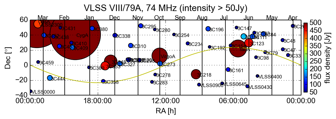
Figure 3: Sky map of intense radio sources and their location with respect to the Sun. The yellow line shows the path of the Sun during one year. The area of each source represents its flux density. A compact source with a high flux density and a distance of a few 10 degrees is best suited for the calibration of solar data.

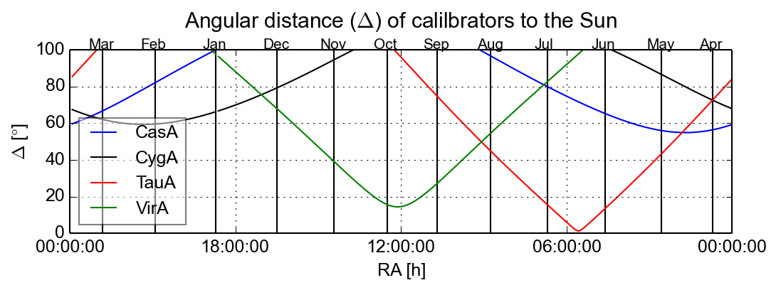
Figure 4: Annual variation of the distance ($\Delta$) of sources with high flux density that are used as calibrator for solar LOFAR data.

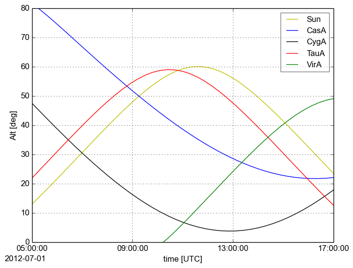
Figure 5: Daily variation of the altitude of solar calibrators. Low altitude observations provide data of lower quality which are also harder to calibrate. The LSDC provides these plots for every day of the year to support the scheduling of observations.

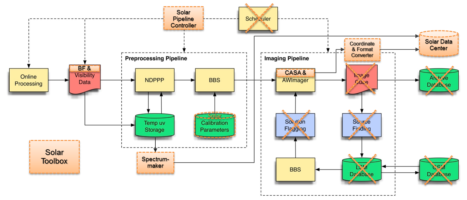
Figure 6: Flowchart of the Standard Imaging Pipeline and the modifications (orange) that lead to the Solar Imaging Pipeline. The data flow starts with the online processing and ends at the Solar Data Center. The crossed out components are not needed for solar imaging. Details of the individual components are described in the text.

3.1.4 High flux density of solar radio emission

Another difference exists with the radio sources that can be used for calibration. For many sky regions detailed sky models exist with a resolution of a few Jy which the Sun passes during a year. But since the Sun emits a flux density of $10^{4}$ Jy or orders of magnitudes more its radiation dominates the signal from these sky regions and is picked up through LOFAR’s side lobes. Consequences:

• Only strong radio sources can serve as calibrators. These sources are Cassiopeia A, Cygnus A, Taurus A and Virgo A (Fig. 3). For this reason solar observations are done with two sub-array pointings. One is directed at the Sun and the other at a suitable calibrator source. This way the calibration coefficients can be obtained from the calibrator data and then applied to the data from the Sun. However, this adds additional constraints for the observation. First the angular distance between the Sun and the calibrator may neither be too small ($<5$ deg) nor too large ($>50$ deg), since otherwise the calibrator will be perturbed by the Sun or the calibration will be perturbed by an imperfect beam model, respectively. Fig. 4 shows the distance ($\Delta$) of the calibrators to the Sun versus time. Second the Sun and the calibrator need to be observed at sufficiently high altitude angles ($>20$ deg) since otherwise their radio emission is too much perturbed by the atmosphere. This condition also excludes observations during winter months from November to February. Fig. 5 shows the altitudes which have to be taken into account for an observation on July 1.

• Similar to the emission from the Sun also the emission from the calibrators effects the solar data. Therefore its influence should be removed by demixing. Demixing is a method in which the contribution from certain radio sources is modeled and subtracted from the data. Unfortunately, demixing often does not work well without a model for the radio emission from the Sun which is not available at pre-processing, when demixing is applied for standard imaging. So demixing is not yet part of imaging of the Sun.

3.1.5 Observations during day time

LOFAR Solar observations have to be done during daytime, preferably at noon. At noon ionospheric scintillation also reach their maximum. Consequence:

• Ionospheric scintillation causes different phase delays for different atmospheric regions the radio signals pass on their way to different LOFAR stations. This leads to calibration and imaging errors, more severely during day time than during night time. This is also another reason for a lower image quality of solar observations than of other observations which are usually taken during night time.

3.2 The solar data processing

The solar imaging pipeline was developed according to the above criteria. The outline is shown in Fig. 6. It shows the data flow and in orange color the modifications from the Standard Imaging Pipeline. The individual steps and components are discussed below.

3.2.1 Online processing

The LOFAR data from all stations is correlated at a computer cluster in Groningen. This correlates the data in real-time and stores it at a temporary storage for a later processing. Currently either low or high-band antenna data is recorded at several equidistant frequencies. Each of these frequency subbands has a bandwidth of 195 kHz and a subdivision into 64 channels. During solar observations also beam-formed data for dynamic spectroscopy is recorded in addition to visibility data which is used for standard imaging.

3.2.2 Temporary storage and data formats

The immediate processing of the data as shown in Fig. 6 is not yet realized but a planned processing option for the future. Instead the data is currently sent to a temporary storage. The imaging and spectroscopic data is recorded in CASA Measurement Sets (MS, McMullin et al. [2007]) and LOFAR’s beam-formed format [Stappers et al., 2011] with an HDF5 container [The HDF Group, 1997-2014] respectively. An MS contains the data of only one subband. The raw data rate scales with the number of channels recorded and is roughly 30 times larger than data with a single channel average. The typical size for the latter is about 1 GB for 10 hours of data with time resolution of 1s. The corresponding JPEG images and thumbnails have about the same size, while the FITS images need about three times as much. The size of beam-formed data scales with the time resolution and number of channels. It is similar to the size of one MS while providing a higher resolution. In summary a typical solar observation of a few hours produces a few TB of data.

3.2.3 New Default Pre-Processing Pipeline (NDPPP)

The first step in the pre-processing of imaging data is done with the New Default Pre-Processing Pipeline (NDPPP). This includes flagging of the channels of the calibrator data for RFI with the AOFlagger [Offringa et al., 2013]. The Sun data are not flagged, to preserve all variable radio features. Subsequently, the channels (excluding edge channel) of all subbands are averaged to one channel per subband and the uv-range is limited to 0-1000 wavelengths.

3.2.4 BlackBoard Selfcal (BBS)

The second step of the pre-processing is the calibration with LOFAR’s BlackBoard Selfcal (BBS) system. Here amplitude and phase corrections are determined for every 30 seconds of calibrator data using a corresponding sky model. The solutions are then transferred to the data from the Sun. Alternatively also two Gaussian sky models of the Sun for low- and high-bands have been developed which can be used for direct calibration of the data from the Sun. However this calibration is less accurate because of the extension of the model only short baselines can be calibrated. Also the determination of the astrometric position is limited to a few arcmin because of the asymmetric variability of the corona.

3.2.5 Solar calibration parameters

BBS is controlled through certain configuration parameters. The specific parameters for the Sun are derived from the standard imaging parameters and are included in the Solar Imaging Pipeline. They are optimized for the calibration of strong calibrator sources and a transfer of the calibration coefficients to the solar data.

3.2.6 Imaging

After the calibration the corrected data is imaged with the multi-scale CLEAN algorithm provided by CASA [McMullin et al., 2007]. The final image is then transformed from equatorial to solar coordinates where the Sun is centered and the Sun’s north pole is oriented upwards. This is done for every time step and frequency. Alternatively the CASA imager can be replaced by the AWImager. The AWImager provides additional correction by the w- and A-projection. The former projection removes the effects of non co-planar baselines in large fields. The latter takes into account a varying primary beam during synthesis observations. However, both corrections are not necessary for the small field of view used in solar observations.

With the CASA imager also images from multiple integration steps can be combined. This so-called aperture synthesis virtually increases the number of baselines by combining data from different times where the antenna positions have shifted because of the Earth’s rotation. Aperture synthesis for the Sun is complicated since its RA/Dec coordinates change while imaging is normally done for a fixed RA/Dec coordinate. Therefore the aperture synthesis was extended for sources with changing RA/Dec coordinates. It can be activated via the “movingsource” option of the CASA imager. With the key word “SUN” every time step of an observation is shifted such that the position of the Sun remains fixed. This avoids smearing of the Sun during longer observations periods of hours.

3.2.7 Self-calibration

Optionally an additional phase-only self-calibration can be applied to selected images. In the standard imaging pipeline a source finding algorithm is applied to the image to find sources not contained in the sky model. These are then added to the sky model and applied in a new calibration. For solar observations a simplified method is used which directly uses the cleaned images as model. Since it does not require assumptions about the sources to find, it is useful where little is known about the radio source morphology. Then imaging is repeated resulting in a reduced noise and increased source brightness. Further self-calibration cycles can be repeated if needed until no further improvement is achieved. This is usually the case after one or two cycles.

3.2.8 Simulation of images

The solar imaging pipeline automatically simulates images of a Gaussian model of the Sun, the point spread function (PSF, Fig. 7) and the contributions from the intense radio sources Cygnus A, Cassiopeia A, Taurus A and Virgo A through side-lobes to the model. This is very instructive for understanding the solar images and their fidelity for a given array configuration. The simulated images are accessible through the LOFAR Solar Data Center described in section 4.

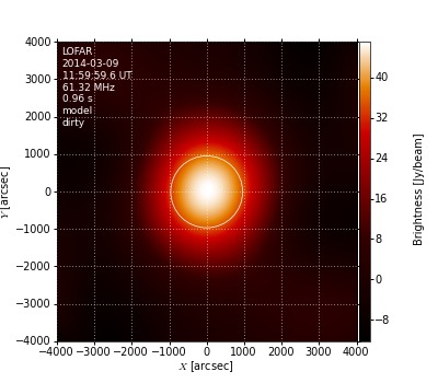
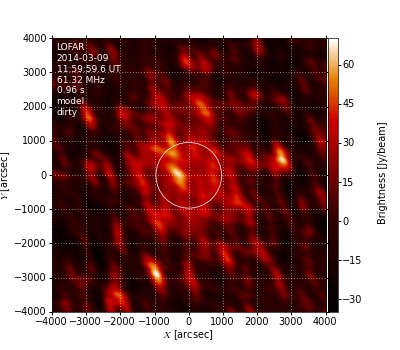
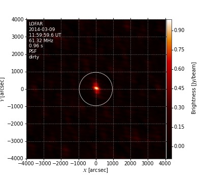
Figure 7: Simulated radio images of a two-dimensional Gaussian model of the Sun (top), this model with side-lobe contributions from the four strong radio sources mentioned in section 3.2.8 (middle) and of the PSF (bottom) for an observation on March 9, 2014.

3.2.9 Solar Pipeline controller

The Solar Imaging Pipeline controller replaces the scheduler of the standard imaging pipeline. It is capable of the data management, which includes the distribution of data to the LOFAR processing cluster and its collection. It also controls the steps of the solar imaging pipeline the LOFAR data is run through.

3.2.10 Solar toolbox

The solar toolbox contains further programs for various tasks related to the data processing. This includes calculations of solar coordinates and angles, image format conversion, extraction of specific observation periods, job and disk space monitoring, the correction of pointing positions and many other tasks.

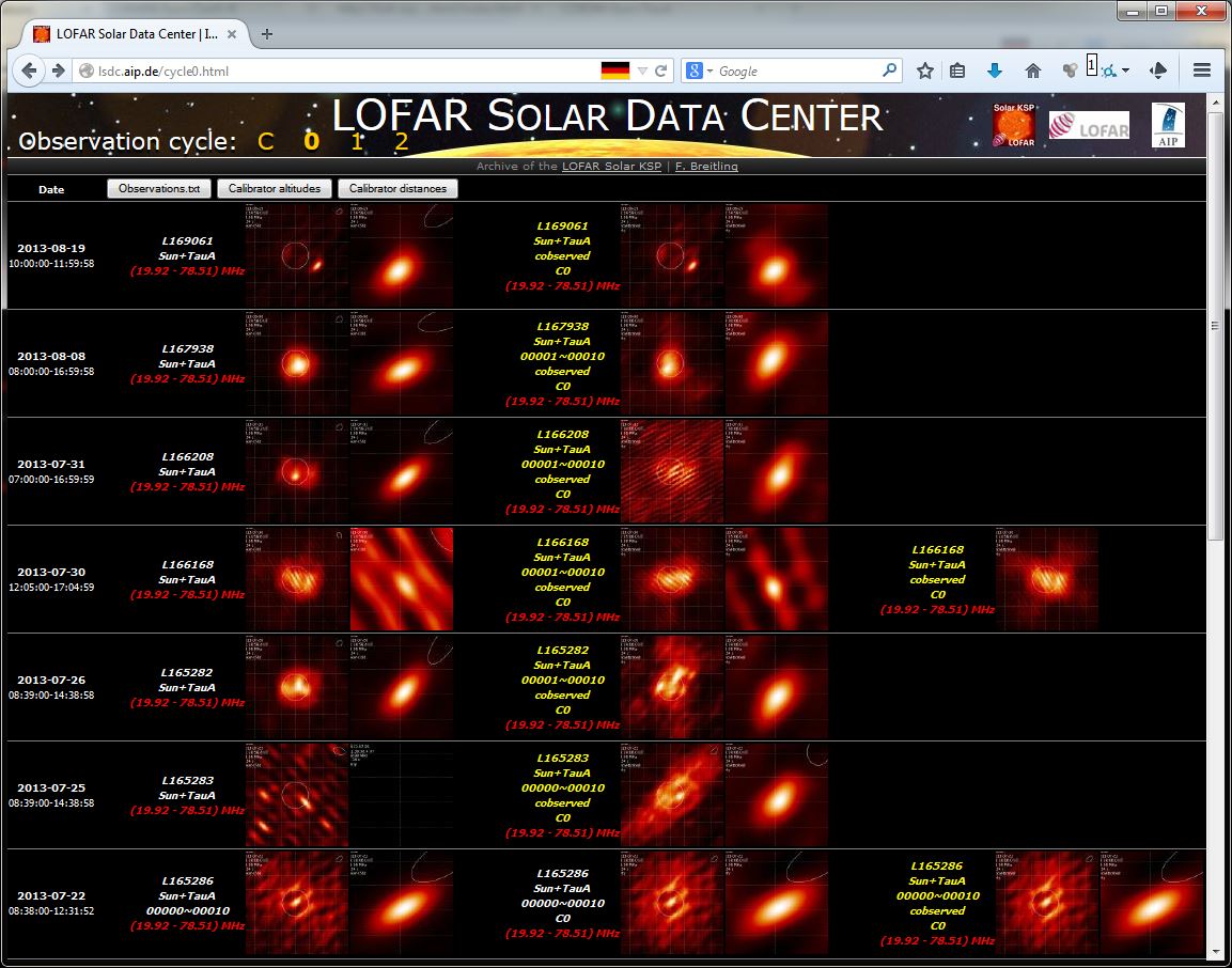
Figure 8: Main page of the LOFAR Solar Data Center showing data from observations cycle 0. The available observations are listed chronologically line by line and linked to their corresponding observation page.

3.2.11 Dynamic spectra

The Solar Imaging Pipeline also provides the spectrum maker for processing beam-formed data. This identifies and excludes channels with a high tenth percentile caused by RFI. It also excludes channels close to the edge of a subband which contain data of low quality. It averages the remaining channels of each subband and scales them to values between 0 and 1. To make the scaling more robust against RFI the highest 1% of the recorded values are ignored for the scaling and truncated to 1. To emphasize the burst signatures the values are gamma corrected. Intermediate values between the different subbands are interpolated.

4 The LOFAR Solar Data Center

The LOFAR Solar Data Center (LSDC) is the archive for LOFAR data products of the Solar KSP. Its software is part of the Solar Imaging Pipeline and it is located and operated at the AIP. It provides a web user interface at http://lsdc.aip.de/ to share LOFAR solar observations with the solar science community. It was designed for browsing through available data, for finding specific observations and for presenting the data products in a way that supports the identification of solar events and their interpretation. To serve this purpose the LSDC is structured as follows.

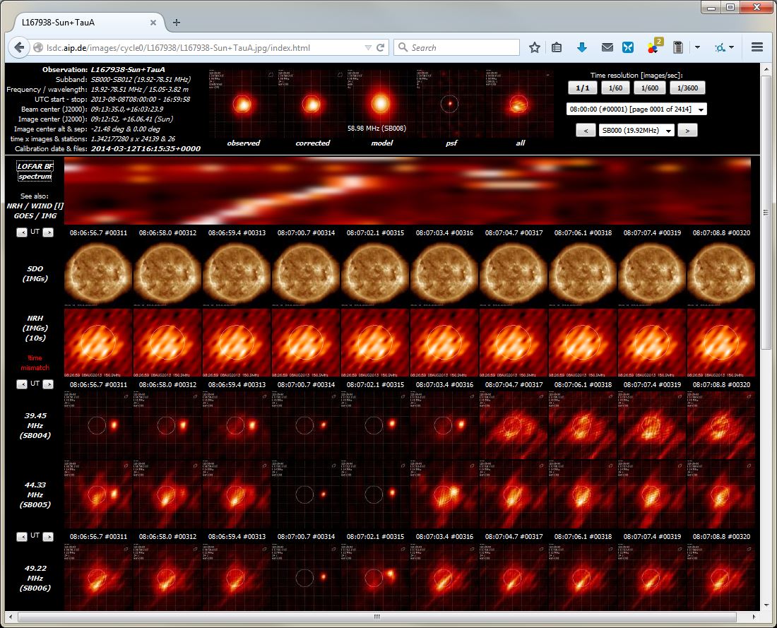
Figure 9: LSDC page of observation L206894 providing observation details, diagnostic images and a navigation box in the first row. Spectra, images from other instruments and images of the individual subbands follow. All images are previews that are linked to their full resolution version. A few solar type III bursts are visible in the dynamic radio spectrum and in the corresponding images, which also show their location.

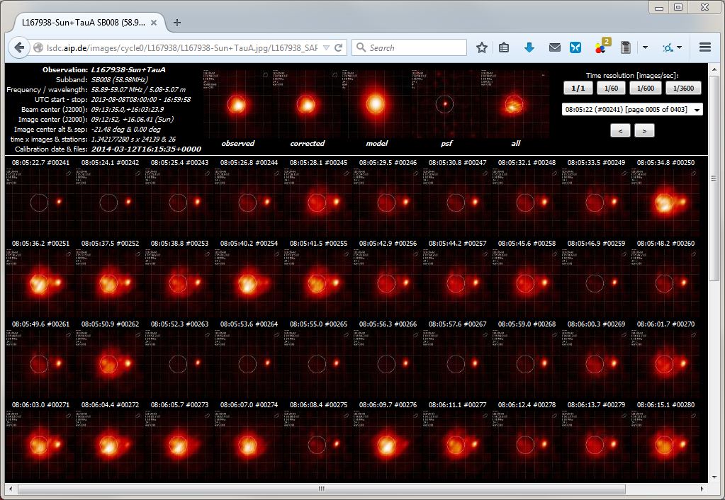
Figure 10: The page of subband 180 (65 MHz) of observation L206894. It can show longer periods of a single subband than the observation page. Here the sudden brightening within seconds in the north east reveals a type III burst. The first row is very similar to the first row of the observation page and has the same functionality.

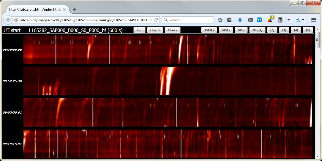
Figure 11: The LOFAR dynamic spectrum page is useful to identify solar events such as solar radio bursts, which are clearly visible as drifting broadband peaks. The top row provides further information and functionality explained in the text.

4.1 Main page

The LSDC is entered through the main page shown in Fig. 8. It shows a header with the title, icons and a menu at the left for switching between different observation cycles to be displayed in the main section of the page. Currently available options are C for the commissioning cycle and 0 to 2 for the regular operation cycles. Here cycle 0 is selected for the further discussion. The main section starts with a row of three buttons. They link to the list of available observations and to plots of the altitudes of the solar calibration sources (Fig. 5) and their distances to the Sun (Fig. 4). The plots provide useful information for selecting calibrators for observations and the data processing. Next a chronological table follows with the available data of the observation cycle. Each row represents one observation and its available data products. It starts with the observation date including start and end time followed by the results from different processing strategies. Each result contains information about the observation ID, the target and calibrator source, possible additional information regarding the calibration and cleaning parameters, the observation frequency and a preview images of the Sun and the calibrator. Each image links to the corresponding observation page with all related data products.

4.2 Observation page

The observation pages provide access to the available data products for viewing and downloading. It also provides a control box to browse through them. An example is Fig. 9 which represents observation L206894. It is organized in rows, each showing the image sequence of a subband. However the first four rows are different:

1. The first row starts with a summary of observation specifications and a link to configuration and logfiles from the processing. The following five diagnostic images give an idea about the data and calibration quality. They show the un-calibrated data, the calibrated data, a simulated model and the point spread function (PSF) for the time step at the middle of the observation. The fifth image is integrated over the complete observation period. The row ends with the control box for browsing through the data. It starts with four buttons to select different time resolutions that shows every first, 60th, 600th and 3600th image. The drop-down menu in the next line lets the user jump directly to a specific time range. The arrow buttons in the line below steps back or forward in time. The last drop-down menu in this last line opens the page of a selected subband in a new window.

2. The second row shows the dynamic radio spectrum by LOFAR. It also provides links to dynamic spectra from the Nancay Decameter Array [Lecacheux, 2000], the WIND satellite [Bougeret et al., 1995] and the Geostationary Operational Environmental Satellites (GOES).

3. The third row serves as a time axis showing the image numbers and recording times. It also contains navigation buttons to step one page back or forward. It repeats after every two image rows.

4. The fourth row shows extreme ultraviolet images of the lower corona from SDO [Lemen et al., 2012] with a time resolution of minutes.

5. The fifth row shows the images from the Nancay Radio Heliograph [Kerdraon & Delouis, 1997] at 151 MHz with a time resolution of 10 s.

6. The sixth row shows the same time axis as the third row.

7. From the seventh row on the LOFAR images from the different subbands follow with increasing frequency.

The images are only previews linked to the full resolution images. The page also contains links to the individual subband pages and to the dynamic spectrum page.

4.3 Subband page

The subband page shows images of a single subband and so can display a longer image sequence. This is useful for studying the temporal evolution of a solar radio event over longer period. Fig. 10 shows subband 180 (65 MHz) of observation L206894 as an example. The first row is very similar to the first row of the observation page and provides the same functionality.

4.4 Dynamic spectrum page

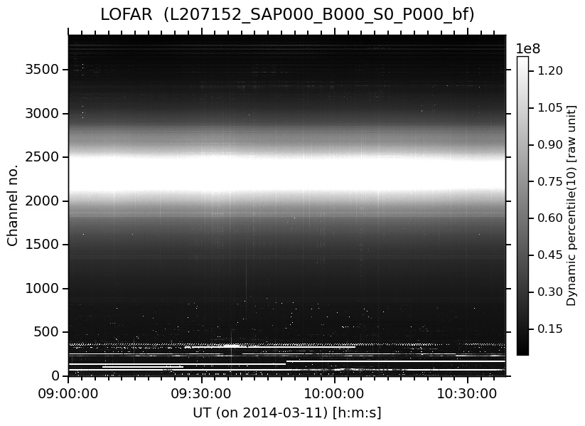
Figure 12: Dynamic spectrum of the channels of LOFAR beam-formed data. This is useful to check the data for RFI.

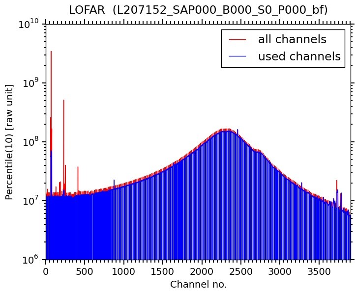
Figure 13: Channel values of LOFAR beam-formed data. Channels with values within the tenth percentile of one subband and channels close to the edge of a subband (red) are flagged and removed. The remaining channels (blue) are used to build the LOFAR dynamic spectrum.

The dynamic spectrum page is shown in Fig. 11. Its purpose is to display the LOFAR dynamic spectra next to each other to cover a long time range. This arrangement is very useful for identifying solar radio bursts. Each row continues the time range covered by the previous row. Each spectrum is only a preview and links to its full resolution version. The first row shows the observation id and buttons with additional functionality. One provides further information about the observation settings, two others show RFI (Fig. 12 and 13), some can change the time resolution of the spectra and others can select pages of a certain time range.

5 Conclusion

LOFAR is a new radio interferometer for dynamic imaging spectroscopy that can be used for observations of the Sun. Solar observations are managed by the LOFAR Key Science Project “Solar Physics and Space Weather with LOFAR”, which has developed the Solar Imaging Pipeline and the Solar Data Center for processing the LOFAR data and providing access to the data product by the solar physics community. The Solar Imaging Pipeline builds upon the Standard Imaging Pipeline and differs in several ways as required by solar radio observations. The Solar Data Center is the archive of the Solar KSP and is located at the AIP. It provides access to processed data from solar observations through a web interface. The LOFAR spectra and images of the Sun have been compared with other observations by other instruments such as the Nancay Radio Heliograph and the Nancay Decameter Array [Lecacheux, 2000] and good agreement has been found. The successful verification permits the usage of solar LOFAR observations for scientific studies, which will be discussed in forthcoming publications.

References

References

- Bastian [2004] Bastian, T. S. 2004, Planet. Space Sci., 52, 1381
- Bougeret et al. [1995] Bougeret, J.-L. et al. 1995, Space Sci. Rev., 71, 231
- Breitling et al. [2011] Breitling, F., Mann, G., & Vocks, C. 2011, Planetary, Solar and Heliospheric Radio Emissions (PRE VII), 373, 1511.03123
- Dulk [2000] Dulk, G. A. 2000, Washington DC American Geophysical Union Geophysical Monograph Series, 119, 115
- Heald et al. [2011] Heald, G. et al. 2011, Journal of Astrophysics and Astronomy, 32, 589, 1106.3195
- Kerdraon & Delouis [1997] Kerdraon, A., & Delouis, J.-M. 1997, in Lecture Notes in Physics, Berlin Springer Verlag, Vol. 483, Coronal Physics from Radio and Space Observations, ed. G. Trottet, 192
- Lecacheux [2000] Lecacheux, A. 2000, Washington DC American Geophysical Union Geophysical Monograph Series, 119, 321
- Lemen et al. [2012] Lemen, J. R. et al. 2012, Sol. Phys., 275, 17
- Mann [2006] Mann, G. 2006, Washington DC American Geophysical Union Geophysical Monograph Series, 165, 221
- Mann [2010] ——. 2010, Landolt Börnstein, 216
- Mann et al. [1999] Mann, G., Jansen, F., MacDowall, R. J., Kaiser, M. L., & Stone, R. G. 1999, A&A, 348, 614
- Mann et al. [2011] Mann, G., Vocks, C., & Breitling, F. 2011, Planetary, Solar and Heliospheric Radio Emissions (PRE VII), 507
- McLean [1985] McLean, D. J. 1985, in Solar Radiophysics: Studies of Emission from the Sun at Metre Wavelengths, ed. D. J. McLean & N. R. Labrum (Cambridge and New York, Cambridge University Press), 37–52
- McMullin et al. [2007] McMullin, J. P., Waters, B., Schiebel, D., Young, W., & Golap, K. 2007, in Astronomical Society of the Pacific Conference Series, Vol. 376, Astronomical Data Analysis Software and Systems XVI, ed. R. A. Shaw, F. Hill, & D. J. Bell, 127
- Melrose [1985] Melrose, D. B. 1985, in Solar Radiophysics: Studies of Emission from the Sun at Metre Wavelengths, ed. D. J. McLean & N. R. Labrum (Cambridge and New York, Cambridge University Press), 177–210
- Offringa et al. [2013] Offringa, A. R. et al. 2013, A&A, 549, A11, 1210.0393
- Stappers et al. [2011] Stappers, B. W. et al. 2011, A&A, 530, A80, 1104.1577
- Suzuki & Dulk [1985] Suzuki, S., & Dulk, G. A. 1985, in Solar Radiophysics: Studies of Emission from the Sun at Metre Wavelengths, ed. D. J. McLean & N. R. Labrum (Cambridge and New York, Cambridge University Press), 289–332
- Tasse et al. [2013] Tasse, C., van der Tol, S., van Zwieten, J., van Diepen, G., & Bhatnagar, S. 2013, A&A, 553, A105, 1212.6178
- The HDF Group [1997-2014] The HDF Group. 1997-2014, Hierarchical Data Format, version 5, http://www.hdfgroup.org/HDF5/
- van Haarlem et al. [2013] van Haarlem, M. P. et al. 2013, A&A, 556, A2, 1305.3550
- Warmuth & Mann [2005] Warmuth, A., & Mann, G. 2005, in Lecture Notes in Physics, Berlin Springer Verlag, Vol. 656, Lecture Notes in Physics, Berlin Springer Verlag, ed. K. Scherer, H. Fichtner, B. Heber, & U. Mall, 49
- Wild [1950] Wild, J. P. 1950, Australian Journal of Scientific Research A Physical Sciences, 3, 541