Polaritonic Rabi and Josephson Oscillations

Abstract

The dynamics of coupled condensates is a wide-encompassing problem with relevance to superconductors, BECs in traps, superfluids, etc. Here, we provide a unified picture of this fundamental problem that includes i) detuning of the free energies, ii) different self-interaction strengths and iii) finite lifetime of the modes. At such, this is particularly relevant for the dynamics of polaritons, both for their internal dynamics between their light and matter constituents, as well as for the more conventional dynamics of two spatially separated condensates. Polaritons are short-lived, interact only through their material fraction and are easily detuned. At such, they bring several variations to their atomic counterpart. We show that the combination of these parameters results in important twists to the phenomenology of the Josephson effect, such as the behaviour of the relative phase (running or oscillating) or the occurence of self-trapping. We undertake a comprehensive stability analysis of the fixed points on a normalized Bloch sphere, that allows us to provide a generalized criterion to identify the Rabi and Josephson regimes in presence of detuning and decay.

I Introduction

A superconductor can be described by an order parameter, that reduces in the simplest formulation the dynamics of such a complex object to a simple complex number landau50a . The question of what happens with the phases of two superconductors put in contact through an insulating barrier led Josephson to predict in 1962 with elementary equations that a supercurrent should flow between them, driven by their phase difference josephson62a . The phenomenon was quickly observed anderson63a and became emblematic of broken symmetries and quantum effects at the macroscopic scale. It was soon speculated that a similar phenomenology should be observed with other macroscopically degenerated quantum phases, such as superfluids or Bose–Einstein condensates, even before the latter were experimentally realized javanainen86a . The role of the phase as the driving agent of quantum fluids was brought to the fore by Anderson anderson66a who identified “phase slippage” as a source of dissipation varoquaux15a . Notably, in the case of BECs, the first transposition of this physics was considering non-interacting particles javanainen86a and the role of the phase difference as a drive for the superflow was the focus of attention. The question of the phase of macroscopically degenerate quantum states remained anchored in the phenomenon but also took a separate route of its own leggett91a ; castin97a ; molmer97a , that is still actively investigated to this day anton14a ; javanainen15a .

The Josephson effect itself, on the other hand, was put on its theoretical foothold by Leggett who defines it as the dynamics of $N$ bosons “restricted to occupy the same two-dimensional single particle Hilbert space” leggett01a . Leggett introduced three regimes for such systems depending on the relationship between tunelling and interactions, namely the Rabi (non-interacting), Josephson (weakly-interacting) and Fock (strongly-interacting) regimes leggett99a . “Tunneling” refers to linear coupling between the condensates (quadratic in operators) while “interactions” refer to a nonlinear self-particle quartic term. In this sense, Josephson’s physics is a limiting case of the Bose–Hubbard model veksler15a , although the name retained a strong bond with superconductors barone_book82a , possibly due to the important applications it found as a quantum interference device jaklevic64a ; kleiner04a or merely for historical reasons (the Josephson–Bardeen debate on the existence of the effect is one highlight of scientific controversies mcdonald01a ). To mark this difference, one speaks of “Bosonic Josephson junctions” (BJJ) for bosonic implementations of the Josephson dynamics gati07a . This typically relates to condensates trapped in two wells, but due to its fundamental and universal character as formulated by Leggett, numerous platforms exhibit the effect. A pioneering report came from superfluids pereverzev97a . For proper BECs, a so-called “internal” Josephson effect was deemed “more promising” with alkali gases by involving different hyperfine Zeeman states rather than a straightforward coupling between two spatially separated condensates leggett99a . Eventually, the Josephson oscillation was observed in a single junction of BEC albiez05a . In this text, we consider another platform that can host Bose condensates: microcavity polaritons kavokin_book11a . These systems having demonstrated Bose–Einstein condensation kasprzak06a and superfluid behaviour amo09a , are natural candidates to implement the Josephson physics of coupled condensates—furthermore, in strongly out-of-equilibrium open systems—and several theoretical proposals have been made sarchi08a ; wouters08b ; shelykh08a , followed by experimental demonstrations, both in the linear (Rabi) lagoudakis10a and nonlinear (self-trapping) abbarchi13a regime. The polariton implementation of Josephson effects is increasingly investigated aleiner12a ; pavlovic13a ; khripkov13a ; racine14a ; gavrilov14a ; zhang14d ; ma15a ; rayanov15a ; zhang15a . Recently, it was observed that polaritons are predisposed for Josephson physics from the very nature of their light-matter composition voronova15b , exhibiting the internal type of such Josephson dynamics where the exchange is not between two spatially separated condensates but between the two internal degrees of freedom that make up the polariton, namely, its exciton and photon components. This is an adequate picture, since condensates of polaritons are also condensates of photons and excitons dominici14a , with their Rabi coupling acting as the tunneling. Interactions are then for the excitonic component only, bringing a variation on the atomic counterpart in space, and detuning of the free energies between the modes acts as the external potential, so the analogy is essentially complete. Bringing the framework of Josephson dynamics to light-matter coupling sheds a new light on polariton Rabi oscillations, in particular pointing out the phase dynamics between the modes, which has been essentially ignored in the description of such problems when considered at the level of coupled oscillators agarwal86a ; carmichael89a ; laussy09a rather than macroscopic wavefunctions. Since the latter are reduced to an order parameter that does not need in most cases vary in space (but see Refs. liew14a, ; colas16a, ), both frameworks are tightly related, and we explore such connections in the following. Specifically, we focus on the general case where both detuning and different on-site interactions are possible, also in presence of decay and pumping, as befit light-matter interaction problems in dissipative quantum optics. We show how this wider picture blurs the line between Rabi and Josephson dynamics, or, rephrased more positively, provides an elegant and natural physical picture that brings the two regimes closer together. We provide a general criterion to take into account the new parameters and that should be considered to claim the Josephson regime beyond the simple observation of oscillations or of a running phase.

II Theory

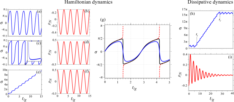
Figure 1: Dynamics of the relative phase $\sigma$ and population imbalance $\rho$ in a variety of scenarios of the pure Rabi regime: (a–b) oscillating-phase regime with sinusoidal cillations, with parameters $\rho_{0}=0.3N$, $\sigma_{0}=0$ and $\delta=-0.5$. (c–d) oscillating-phase regime with strongly anharmonic oscillations of the phase. A zoom in inset shows that the phase is continuous. The oscillations in the population remain sinusoidal. Parameters: $\rho_{0}=0.44N$, $\sigma_{0}=0$ and $\delta=-0.5$. (e–f) Running-phase regime (or discontinuous jumps if not unwrapped). Parameters: $\rho_{0}=0.48N$, $\sigma_{0}=0$ and $\delta=-0.5$. (g) Transition from the oscillating-phase (solid lines) to the running phase (dashed, not unwrapped) observed as a function of the population imbalance $\rho_{0}$, from $\rho_{0}=0.25N$ (smooth blue curve) below threshold to $\rho_{0}=.305N$ (red–dashed line) above, passing by $\rho_{0}=0.299N$ (black, kinky line) very close to threshold (from below). Other parameters are: $\delta=-1$ and $\sigma_{0}=0$. (h) Relative phase and (i) population imbalance in the dissipative regime (with decay and without pumping nor interactions). There is a transition from the oscillating-phase to the running-phase regime at $t_{1}$ and back at $t_{2}$, with no notable feature in the population imbalance. Parameters: $\rho_{0}=-0.2N$, $\sigma_{0}=\pi$, $\delta=-1$, $\gamma_{a}=0.22g$ and $\gamma_{b}=.02g$, in which case $t_{1}\approx 6.9g$ and $t_{2}\approx 28g$.

The dynamics of the Bosonic Josephson effect has been considered extensively by Raghavan et al. raghavan99a in a form suitable for our discussion, including some considerations of dissipation marino99a (see Ref. gati07a, for a review). We now briefly introduce the main points and notations. We consider the coupling between two weakly-interacting Bose fields, $a$ (photons) and $b$ (excitons), with possibly different free energies $\epsilon_{a,b}$, ruled by the Hamiltonian:

$$H =H_{0}+V\,,$$ (1a)

$$H_{0} =\epsilon_{a}a^{\dagger}a+\epsilon_{b}b^{\dagger}b+g(a^{\dagger}b+b^{\dagger}a)\,,$$ (1b)

$$V =v_{b}(b^{\dagger}b^{\dagger}bb)+v_{a}(a^{\dagger}a^{\dagger}aa)\,.$$ (1c)

Of course our results and conclusions apply to other systems than the internal Josephson dynamics of light-matter coupling, as long as they are well described by Eqs. (1), but we will keep this terminology for convenience. In a Josephson workframe, $a$ and $b$ are ground state annihilation operators and the averages $\langle a\rangle$ and $\langle b\rangle$ are order parameters ($c$-numbers) for the two condensates (we will note $n_{a}\equiv\langle{a^{\dagger}}a\rangle$ and $n_{b}\equiv\langle{b^{\dagger}}b\rangle$ the populations of each mode). The dynamics can be described in terms of i) the population imbalance $\rho\equiv(\langle a^{\dagger}a\rangle-\langle b^{\dagger}b\rangle)/2=(n_{a}-n_{b})/2$ between the two modes and ii) their relative phase $\sigma=\arg{\langle a^{\dagger}b\rangle}$. Note that the relative phase is, strictly speaking, $S\equiv\arg(\langle a\rangle-\langle b\rangle)$ while we define it here as $\sigma$, the argument of a first-order cross-correlation. This is done for greater generality as it allows us to describe all types of quantum states for coupled harmonic oscillators, including mixed states, as will be discussed in section V. For coherent states (describing ideal condensates), $S=\sigma$, and our convention thus causes no loss of generality. Note that such mean-field approximations that provide the pillars for the physics at play have been relaxed in recent years and exact (numerical) solutions are now available sakmann09a ; chuchem10a that, interestingly, depart considerably from the established picture, in particular regarding the role of the phase. In our mean-field approximation, where $\langle a^{\dagger}bb^{\dagger}b\rangle\approx\langle a^{\dagger}b\rangle\langle b^{\dagger}b\rangle$ and $\langle a^{\dagger}ba^{\dagger}a\rangle\approx\langle a^{\dagger}b\rangle\langle a^{\dagger}a\rangle$ (this assumes that the states remain coherent states), the two observables are ruled by the following equations of motion raghavan99a ; voronova15b :

$$\partial_{t}(\rho/N) =F_{1}(\rho,\sigma)\equiv -\sqrt{1-4(\rho/N)^{2}}\sin(\sigma)\,,$$ (2a)

$$\partial_{t}\sigma =F_{2}(\rho,\sigma)\equiv \Delta E-2(\rho/N)\Lambda+{}$$ (2b)

$${}+\frac{4\rho/N}{\sqrt{1-4(\rho/N)^{2}}}\cos(\sigma)\,,$$

where we introduce the notation $F_{1,2}$ for future convenience. $N\equiv\langle a^{\dagger}a\rangle+\langle b^{\dagger}b\rangle$ is the total number of particles, $\delta=(\epsilon_{a}-\epsilon_{b})/g$ is the bare modes detuning and we highlight two particular parameters of importance to describe the dynamics, an effective detuning $\Delta E$ and an effective blueshift $\Lambda$:

$$\Delta E \equiv-\delta+N(v_{b}-v_{a})/g\,,$$ (3a)

$$\Lambda \equiv(v_{a}+v_{b})N/g\,.$$ (3b)

Equations (2) are the so-called BJJ equations gati07a that describe the dynamics of coupled BECs. They differ in several aspects from Superconducting Josephson Junction equations but also bear enough resemblances to lead to similar physics. Voronova et al. voronova15b recently reported a peculiar phase dynamics of BJJ when including detuning, even in the linear regime: the phase oscillations are strongly anharmonic and possibly even get in a regime of phase-jumping (or freely running phase if unwrapped). This is noteworthy as reminiscent of the Josephson dynamics, i.e., driven by interactions. Without interactions, oscillations in populations remain harmonic for all detunings, indeed with some renormalization of frequencies and nonzero imbalance, as can be expected from the conventional Rabi coupling picture out of resonance. Particular cases of this time dynamics for $\rho$ and $\sigma$ are shown in Fig. 1. In panel (a) and (c), $\sigma$ oscillates in time, while in panel (e), $\sigma$ is running. Note how in panel (c), close to the frontier between the two-cases, the phase is highly deformed from harmonic oscillations. An inset shows that the oscillation is continuous even though it becomes very sharp. This is also seen in Fig. 1(g) for three regimes around the transition, showing how the phase abruptly changes from steep oscillations of $\pi$ amplitudes (solid lines) to $2\pi$ phase jumps (dashed line). In panel (e), we have unfolded the phase for clarity. In all cases, particles transfer harmonically between the two states as oscillations in $\rho$ show. For such pure Hamiltonian dynamics, initial conditions as well as detuning determine the possible regimes of relative phase. There follows a rich phase diagram that can be characterized analytically voronova15b in the linear or weakly interacting regime. Here it must be stressed again that the same phenomenology that is usually attributed to Josephson dynamics is observed without interactions, that is, in the pure Rabi regime. This calls to reconsider what is meant, precisely, by Josephson and Rabi dynamics. We clarify this point below.

In the quantum-optical mindset, dissipation is an essential part of the dynamics agarwal84a ; carmichael89a . This is also an ingredient that is important to describe short-lived polaritons. To do so, the formalism is upgraded from an Hamiltonian to a Liouvillian description, leading to a master equation for the density matrix $\varrho$: carmichael_book02a ; delvalle_book10a :

$$\partial_{t}\varrho=i[\varrho,H]+ \sum_{c=a,b}\frac{\gamma_{c}}{2}(2c\varrho c^{\dagger}-c^{\dagger}c\varrho-\varrho c^{\dagger}c)+$$ (4)

$$\sum_{c=a,b}\frac{p_{c}}{2}(2c\varrho c^{\dagger}-c^{\dagger}c\varrho-\varrho c^{\dagger}c)\,,$$

where $\gamma_{c}$ and $p_{c}$ are decay and incoherent pumping rates for the states $c=a,b$. Then, Eqs. (2) in this dissipative regime and for coherent states become:

$$\partial_{t}(\rho/N) =-\sqrt{1-4(\rho/N)^{2}}\sin(\sigma)+\frac{1}{2}\Gamma_{-}-2(\rho/N)^{2}\Gamma_{-}\,,$$ (5a)

$$\partial_{t}\sigma =\Delta E-2(\rho/N)\Lambda+\frac{4\rho/N}{\sqrt{1-4(\rho/N)^{2}}}\cos(\sigma)\,,$$ (5b)

where (with $p_{a}=p_{b}=0$ in the case with only decay):

$$\Gamma_{\pm}\equiv\frac{1}{2}[(p_{a}-\gamma_{a})\pm(p_{b}-\gamma_{b})]\,.$$ (6)

One example of the dissipative Rabi dynamics is shown in Fig. 1(h–i). Remarkably, one observes a switching in time between the oscillating and running phase regimes. This switching is caused by the decay and depends on the initial condition as well as detuning. The switching happens if the occupation in one state becomes exactly zero, with all the population residing in the other state, although this is not a necessary condition. When this occurs, the phase of the emptied state becomes ill-defined and so does the relative-phase. Such a change of regime can appear two times, as shown in the figure, a single time or none. In any case, the system always ends up in the regime of oscillating phase, except at resonance where the running mode can last forever. There is therefore only one switching when the initial condition and detuning are such that the dynamics starts in the running phase mode. These are mere statements of the facts. We will explain the reason for this peculiar behaviour in the following and it will become clear that such an apparently rich phenomenology is in fact trivial and bears no connection to Rabi and Josephson dynamics.

Equations (2) and (5) are the traditional form for the (bosonic) Josephson dynamics, coupling population imbalance and relative phase in a way that supports the notion that one drives the other. This form conceals, however, the more fundamental structure that underpins the relationship between the key variables: population imbalance indeed, but the full complex correlator $\langle{a^{\dagger}}b\rangle$ rather than merely its phase (once the connection is understood, however, one can indeed limit to the phase). The dynamics is thus put in full view geometrically in the $(\rho,\langle{a^{\dagger}}b\rangle)$ space. Since $\langle{a^{\dagger}}b\rangle$ is complex, the space is three-dimensional. The trajectories can be obtained from the full set of equations:

$$\partial_{t}\langle a^{\dagger}b\rangle=(i(\delta)+\Gamma_{+})\langle a^{\dagger}b\rangle-i\langle a^{\dagger}a\rangle+i\langle b^{\dagger}b\rangle$$

$$-2iv_{b}\langle a^{\dagger}bb^{\dagger}b\rangle+2iv_{a}\langle a^{\dagger}ba^{\dagger}a\rangle\,,$$ (7a)

$$\partial_{t}\langle a^{\dagger}a\rangle=-i\langle a^{\dagger}b\rangle+i\langle b^{\dagger}a\rangle+(p_{a}-\gamma_{a})\langle a^{\dagger}a\rangle+p_{a}\,,$$ (7b)

$$\partial_{t}\langle b^{\dagger}b\rangle=i\langle a^{\dagger}b\rangle-i\langle b^{\dagger}a\rangle+(p_{b}-\gamma_{b})\langle b^{\dagger}b\rangle+p_{b}\,.$$ (7c)

Diagonalizing these equations, we get one key result for the dynamics:

$$|\langle{a_{\theta}^{\dagger}}b_{\theta}\rangle|^{2}+\rho_{\theta}^{2}=({N(t)}/{2})^{2}+\mathcal{P}(t)\,,$$ (8)

where:

$$\mathcal{P}(t)=-\exp(2\Gamma_{+}t)\int_{0}^{t}\exp(-2\Gamma_{+}t^{\prime})(p_{a}n_{b}+p_{b}n_{a})dt^{\prime}\,.$$ (9)

This result holds even in the interacting case (with $v_{a}\neq 0$ and/or $v_{b}\neq 0$), but since the Hamiltonian then needs be diagonalized at all times, this is just a formal way to rewrite the equation. In other cases, the geometric nature of the dynamics is captured. Here, the main, albeit obvious, argument is the introduction of the generic equation for $\theta$, the mixing angle between exciton and photons, describing a change of basis:

$$a_{\theta} =\cos(\theta)a+\sin(\theta)b\,,$$ (10a)

$$b_{\theta} =-\sin(\theta)a+\cos(\theta)b\,,$$ (10b)

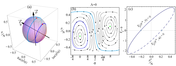
Figure 2: (a) The dynamics of two coupled condensates is clearly understood on a Bloch sphere. The polariton basis defines an axis $\vec{\rho}_{\theta}$ around which the pure Rabi dynamics evolves as a simple circle, whose distance from the center is determined by the quantum state, with polaritons at the poles and the full-amplitude Rabi oscillations between the dressed states as the equator. At resonance, $\delta=0$, $\vec{\rho}$ and $\vec{\rho}_{\theta}$ are orthogonal. parameters are the same as Fig 1. (b) Projection of the dynamics of the two cases in panel (a) on the $(\rho,\sigma)$ space, superimposed on the streamlines of the dynamical system. There are two centers, displayed as green dots, located at $\sigma=0$ and $\sigma=\pi$. (c) The fixed points are solutions of $F_{2}(\rho^{*},\sigma^{*})=0$, that is, the intersection of the curve with the $x$ axis, indicated by open circles. The solid line corresponds to $\sigma=0$ and the dashed one to $\sigma=\pi$. The detuning was taken as $\Delta E=0.5$.

where $\cos(\theta)=\sqrt{1/2+\delta/2\sqrt{4+\delta^{2}}}$. These operators diagonalize the Hamiltonian (1b) and lead to the simple solution, Eq. (8). In the $(\rho,\langle{a^{\dagger}}b\rangle)$ space, the trajectory is therefore simply that of “circles on a sphere”. In non-Hamiltonian cases, the radius changes in time but solutions remain equally simple if kept on a normalized sphere. This sphere is a counterpart of the Bloch sphere, that describes the dynamics of a two-level system. Here the two levels are the exciton and photon amplitudes dominici14a which yield the parametrization for the Bloch vector $\mathbf{v}$:

$$\mathbf{v}=\frac{2}{N}\left(\frac{\langle a^{\dagger}b+b^{\dagger}a\rangle}{2i},\frac{\langle a^{\dagger}b-b^{\dagger}a\rangle}{2i}\frac{\langle a^{\dagger}a-b^{\dagger}b\rangle}{2}\right)\,.$$ (11)

The typical representation in a $(\rho,\sigma)$ plane gati07a produces instead complex patterns, even in the linear case of simple circular motion, as a result of the transformation involved by projecting from a sphere. In recent years, it has however become more common to represent the Josephson dynamics on its appropriate geometry zibold10a ; chuchem10a ; arXiv_voronova16a .

III Hamiltonian regime

III.1 Dynamics

We first revisit the usual Hamiltonian case with no dissipation, i.e., when $p_{a}=p_{b}=\gamma_{a}=\gamma_{b}=0$. The pure Rabi regime, when $v_{a}$ and $v_{b}$ are zero, admits analytical solution for $\rho$ and the phase voronova15b . Namely, for the population imbalance $\rho$:

$$\rho(t)=\big{\{}\delta\big{(}2\cos(\sigma(0))+\rho(0)\delta)+{}\\ {}+(4\rho(0)-\delta P(0)\cos(\sigma(0))\big{)}\cos(Rt)+{}\\ {}+RP(0)\sin(\sigma(0))\sin(Rt)\big{\}}/R^{2}\,,$$ (12)

where we introduced $P\equiv\sqrt{N^{2}-4\rho^{2}}$ and $R\equiv\sqrt{4+\delta^{2}}$. As for the relative phase $\sigma(t)$ (it can also be obtained from the real and imaginary parts of $n_{ab}=\langle a^{\dagger}b\rangle$):

$$\sigma=-\sin^{-1}(\partial_{t}\rho/P)\,.$$ (13)

This is an exact, albeit obscure, description of the dynamics that is put in full view geometrically on the Bloch sphere. Indeed, the comparison between the particular case Eqs. (12–13) with the general solution Eq. (8) shows the great simplification brought by the geometric representation. The nonlinear case has no closed-form solution to the best of our knowledge although as a two-dimensional dynamical system, its solution are readily obtained numerically (we provide separately an applet to compute the trajectories in both the sphere and projected on the phase-space rahmani16Wolfram ). From Eqs. (12–13), for instance, one can derive the conditions for oscillating or running phase, by considering whether $\sigma(t)$ is bounded in time, in which case the function is oscillating. This is achieved by finding zeros for its derivatives, leading to the following equation for the frontier between the two regimes of phase dynamics as a function of detuning and initial conditions:

$$\rho(0)=N\frac{4\cos^{2}(\sigma(0))-\delta^{2}}{2(4\cos^{2}(\sigma(0))+\delta^{2})}\,.$$ (14)

If $\rho(0)$ is less than the rhs, then the phase is oscillating, otherwise it is running. This perplexing result is easily understood on the Bloch sphere, as shown in Fig. 2(a), where the Rabi dynamics reduces to a simple circle. This circle is concisely and fully described by its normal axis $\vec{\rho}_{\theta}$ and its distance $\rho_{\theta}$ from the equator in this basis. The latter is given, on the normalized sphere, by:

$$\rho_{\theta}=\left(\rho\delta+\frac{2\mathrm{Re}\langle{a^{\dagger}}b\rangle}{R}\right)\frac{1}{RN}\,.$$ (15)

This is a familiar result in quantum-optical terms. In the proper basis—of dressed states—the dynamics is that of the free propagation (circular motion) of uncoupled states. This is determined by the $\vec{\rho}_{\theta}$ axis, around which the dressed states evolve freely (harmonically) at a distance from the equator that is determined by their state (their content of lower and upper polaritons), leading to a linearly increasing phase. We can now explain that what determines the dynamics of the phase (oscillating or running) is simply whether the trajectory on the sphere encircles or not the South–North $\rho$ axis defined by the laboratory observables (i.e., of the bare states). In the proper basis of dressed states, the phase is always running. Bare states on the other hand are the familiar physical objects of the system in which terms it is convenient to think. In our case, they are the exciton and photon modes, and are furthermore those typically observed experimentally (only the photons in most experiments). This laboratory basis is, in the case of optimal strong-coupling, orthogonal to the dressed state basis, with $\vec{\rho}_{\theta}\perp\vec{\rho}$, and the circular motion is observed as a sinusoidal oscillation (a circle observed sidewise) in the general case, or even a saw-tooth function when the quantum state maximizes the amplitudes of oscillations by satisfying $\rho/N=\pm 1/2$ (for instance starting with all polaritons in one mode at $t=0$). This is shown in Fig. 1(a,b) and (e,f) that correspond to the case of Fig. 2(a), namely, as initial conditions: a 50-50 (light blue) superposition of $\theta$-eigenstates and another ratio (in blue), leading to a smaller circle, both normal to the $\vec{\rho}_{\theta}$ axis. As observed in the exciton-photon basis, their $\rho$ and $\sigma$ dynamics is distorted. There is no such distortion for the population imbalance, since the circular motion from any circle on the sphere projected on any normal axis still results in a sine function. However the relative phase is defined by that of the vector that joins the center of the sphere and the circle itself. If the circle lies outside the axis, the phase can remain always unequivocally defined in a $2\pi$ interval, leading to oscillations as the trajectory reaches an apex on the circle and turns back. This is the situation of the blue circle in Fig. 2(a). In the other case where the circle goes round the axis, there is no turning point and the phase increases forever. This is the situation of the light blue circle in Fig. 2(a). It is clear, then, that the dynamics of the phase has no deep meaning of driving a flow of particles. Instead, it pertains to a choice of basis. The oscillating phase regime corresponds to a case where the basis of observables is too far apart from that which is natural for the system and the tilt between them is so large that the phase is distorted into a qualitative different behaviour of oscillations instead of a linear drift. In contrast, the running phase regime is that where the system is described by observables close to the dressed states of the system.

The rationale of Leggett in distinguishing between a Rabi and Josephson regime was to set apart the cases where tunneling $g$ (in our case, Rabi coupling) dominates from that where nonlinearity $v$ dominates. At resonance and for equal interaction on both sites, the exact criterion is to compare $2vN/g$ to unity, ($N$ the total number of particles, $v$ the self-interaction and $g$ the tunneling strength). This is indeed correct but, even in absence of dissipation, is restricted to resonance and equal nonlinearities. Here we provide the general result to set apart the Rabi and Josephson regimes in presence of detuning, which is required in general since detuning may fake a Josephson-looking dynamics even in non-interacting systems.

III.2 Classification of fixed points

As we are dealing with a dynamical system, the standard procedure to classify the possible trajectories is a stability analysis around the fixed points. In the BJJ, the fixed points $\rho^{*}$ and $\sigma^{*}$ are by definition the solutions $F_{i}(\rho^{*},\sigma^{*})=0$ for $i=1,2$ (cf. Eqs. (2)). There are two possible solutions for the phase, $\sigma^{\ast}=0$ and $\sigma^{\ast}=\pi$ (modulo $2\pi$, so that $\sigma^{\ast}=-\pi$ is also a solution in a closed $2\pi$ interval). Solving for the other variable, we exhaust the possible fixed points. Their stability is determined by the eigenvalues $\lambda_{i}$ of the Jacobian Matrix given by:

$$J=\left(\begin{array}[]{*2{c}}‎\partial_{\rho}F_{1}&\partial_{\sigma}F_{1}\\ \partial_{\rho}F_{2}&\partial_{\sigma}F_{2}\end{array}\right)_{(\rho^{\ast},\sigma^{\ast})}\,,$$ (16)

and the type can be mapped on a diagram with axes $\Delta\equiv\lambda_{1}\lambda_{2}$ and $\tau\equiv\lambda_{1}+\lambda_{2}$ strogatz_book94a , as shown in Fig. 3.

III.2.1 Non-interacting case

First, in the non-interacting case, the system admits simple closed-form solutions:

$$\sigma^{*}=0\quad\text{and}\quad\rho^{*}=\frac{N}{2}\frac{\delta}{\sqrt{4+\delta^{2}}}\,,$$ (17a)

$$\sigma^{*}=\pi\quad\text{and}\quad\rho^{*}=-\frac{N}{2}\frac{\delta}{\sqrt{4+\delta^{2}}}\,.$$ (17b)

As is clear on physical grounds, detuning can produce a state with a large population imbalance, which can bear resemblance to macroscopic quantum self-trapping even in absence of interaction. Using the definition of Raghavan et al. raghavan99a that the system is macroscopically self-trapped when its total energy balances the coupling strength, we can find a critical detuning that satisfies this condition in absence of interactions, namely:

$$\delta_{s}=\frac{1-\sqrt{1-4(\rho(0)/N)^{2}}\cos(\sigma(0))}{\rho(0)/N}\,.$$ (18)

Examples of dynamics on the Bloch sphere in this noninteracting case are shown in Fig 2(a) and on the projected $(\rho,\sigma)$ space in Fig. 2(b), with the two fixed points at $\sigma=0$ and $\sigma=\pi$ marked by (green) points. The two orbits show the running and oscillatory phases surrounding these fixed points without being attracted nor repelled by them. In the terminology of dynamical systems, this corresponds to fixed points that are neutrally stable. Geometrically, the fixed points are the intersections with the $x$-axis of the curves shown in Fig. 2(c) (zeros of $F_{2}$).

For the stability that follows from Eq. (16), we find $\lambda_{1}=i\sqrt{4+\Delta E^{2}}$ and $\lambda_{2}=-i\sqrt{4+\Delta E^{2}}$, implying that $\Delta>0$ and $\tau=0$. As a consequence, the two fixed points in the Rabi regime are centers, i.e., they are stable and every near-enough trajectory is closed strogatz_book94a . These are the $\mathrm{H}_{(\Lambda\leq\Lambda_{c})}$ points in Fig. 3 with $\Lambda=0$.

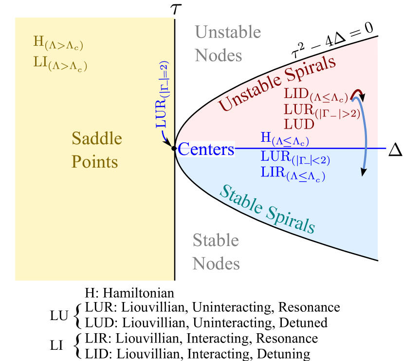
Figure 3: Classification of the fixed points of the dissipative Bosonic Josephson Junction. The axes are the functions $\Delta\equiv\lambda_{1}\lambda_{2}$ and $\tau\equiv\lambda_{1}+\lambda_{2}$ of the Jacobian’s eigenvalues, cf. Eq. (16). Our terminology is spelled out at the bottom of the figure, with (at most) three letters to label each case: first letter is either H (Hamiltonian) or L (Liouvillian) for the cases without or with decay, respectively. Second letter is U (uninteracting) or I (interacting) for the cases without or with self-interactions, respectively. Third letter is R (resonance) or D (detuned) for the cases $\delta=0$ or $\delta\neq 0$, respectively. Further criteria are specified as subscripts. For instance, $\mathrm{LI}_{\Lambda>\Lambda_{c}}$ are dissipative systems with interactions with both zero and nonzero detuning such that $\Lambda>\Lambda_{c}$, in which case these systems have fixed points with saddle instability. The fact that $\Lambda>\Lambda_{c}$ is equivalent to the existence of a saddle fixed point allows to use the latter as a necessary and sufficient criterion for the Josephson regime. The Nodes area, separated from the Spirals by $\tau^{2}-4\Delta=0$, are not accesible. The purple and blue arrows for the points $\mathrm{LUD}_{(|\Gamma_{-}|<2)}$ and $\mathrm{LID}_{(\Lambda\leq\Lambda_{c})}$ mean that these points belong to both the Unstable and Stable Spirals regions. All the cases shown here are for $\Delta E=0$.

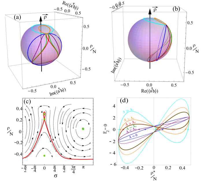
Figure 4: (a) Transition from Rabi to Josephson regime. The Blue circle is the pure Rabi (no interaction) regime. Purple is a Rabi-like interacting case, with $0<\Lambda<\Lambda_{c}$, green is the transition case when $\Lambda=\Lambda_{c}$, red is a Josephson case with $\Lambda$ slightly over $\Lambda_{c}$, orange and cyan are Josephson cases well above $\Lambda_{c}$. (b) Same as (a) but as a side view of the trajectories to show the cases that do encircle or not the $\vec{\rho}$ axis, corresponding to oscillatory and running relative phase, respectively. (c) Phase-space trajectory of the dynamics in the Josephson regime with a saddle point at $\sigma=0$ out of the four fixed points. Each $\Lambda$ yields its own phase-space vector field, in which a trajectory is followed depending on the initial condition. (d) Roots of $F_{2}=0$, that identify the fixed point in the population imbalance for the relative phase $\sigma=0$ mod $2\pi$ (solid line) and $\sigma=\pi$ mod $2\pi$ (dashed line). With increasing $\Lambda$, the number of roots changes from two (Rabi regime) to four (Josephson regime).

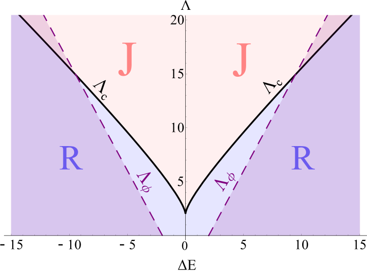
Figure 5: Regions of Rabi (R or blue) and Josephson (J or red) regime as a function of $\Lambda$ and $\Delta E$. The frontier, $\Lambda_{c}$ (solid black line) is given by Eq. (20) and provides the general criterion for the Josephson regime in presence of detuning. The frontier denoted by $\Lambda_{\phi}$ (dashed line) separates the running-phase regime from the oscillating one (shaded area) for the case $(\rho_{0}=0,\sigma_{0}=\pi)$ ($\Lambda_{\phi}$ depends on the quantum state and we show here the case of greatest extent for the running phase). There is some degree of correlation between running phase and Josephson dynamics but neither implies the other.

III.2.2 Interacting case

The general interacting case has fixed points solutions in implicit form:

$$4(\rho^{*}/N)+e^{i\sigma^{*}}(\sqrt{1-4(\rho^{*}/N)^{2}}(\Delta E-2(\rho^{*}/N)\Lambda))=0\,,$$ (19)

also for $\sigma^{*}\in\{0,\pi\}$. Solutions also exist in closed-form but are too bulky to give here. The geometrical solution is, in this case, convenient. It is shown in Fig. 4(d) for various values of $\Lambda_{c}$. From the shape of the curve, one can see that there are two or four fixed points, and this is the criterion one can unambiguously use to define the Rabi and Josephson regimes, respectively. This can be quantified by studying the order of the discriminant of Eq. (19), yielding the Josephson regime when it is higher than quadratic in $\rho$. This leads us to one important result of this text: the generalized criterion for Josephson dynamics. The critical parameter that separates the Rabi from Josephson regimes in the mean-field approximation is thus:

$$\Lambda_{c}=\sqrt{4+\Delta E^{2}+\frac{6(2\Delta E^{2})^{2/3}}{\Xi^{1/3}}+3(2\Delta E^{2})^{1/3}\Xi^{1/3}}\,,$$ (20)

with $\Xi=4+\Delta E^{2}+|4-\Delta E^{2}|$. In the literature, the typical configuration reduces to $\Delta E=0$ and yields $\Lambda_{c}=2$. The diagram in Fig. 5 shows the regions of Rabi (R or blue) and Josephson (J or red) separated by the $\Lambda_{c}$ frontier (black solid line) according to this general criterion. One expects the Josephson regime to occur with increasing effective interaction ($\Lambda$). However, this is strongly countered by detuning, that tends to maintain the Rabi regime with a steep increase of the threshold, that is doubled for a detuning of one time the coupling strength only. In highly detuned conditions, the Rabi regime predominates, even with large values of $\Lambda$.

The fixed points analysis is done for each value of the phase separately. The $\sigma^{\ast}=0$ solution yields eigenvalues $\lambda_{\nu}=\pm i\sqrt{2}{\sqrt{2-\Lambda(1-4\rho^{\ast}\rho^{\ast})^{3/2}}}\big{/}{\sqrt{1-4\rho^{\ast}\rho^{\ast}}}$ ($\nu=1,2$), that imply $\tau=0$ and, as far as $\Lambda\leq\Lambda_{c}$, $\Delta>0$ meaning that the fixed points remain centers (these are the $\mathrm{H}_{(\Lambda\leq\Lambda_{c})}$ points with nonzero $\Lambda$ in Fig. 3). However for $\Lambda>\Lambda_{c}$, one fixed point falls in the region $\Delta<0$ and becomes a saddle point ($\mathrm{H}_{(\Lambda>\Lambda_{c})}$). For $\sigma^{\ast}=\pi$, the eigenvalues read $\lambda_{\nu}=\pm i\sqrt{2}{\sqrt{2+\Lambda(1-4\rho^{\ast}\rho^{\ast})^{3/2}}}\big{/}{\sqrt{1-4\rho^{\ast}\rho^{\ast}}}$ ($\nu=1,2$) which, for all the values of $\Lambda$, results in $\Delta>0$, meaning that all fixed points around $\sigma^{*}=\pi$ remain center points ($\mathrm{H}_{(\Lambda\leq\Lambda_{c})}$), regardless of the strength of the interaction. The existence of one saddle point is thus a criterion to identify the Josephson regime in presence of detuning. On Fig. 3) is also superimposed as a shaded area the region of oscillating phase for the case $\rho_{0}=0$ and $\sigma_{0}=\pi$ (each initial condition yields its own boundary) separated from the region of running phase by the dashed purple line $\Lambda_{\phi}$. While there is a correlation between the running phase and the Josephson regime, one neither implies nor is implied by the other.

Examples of orbits on the Bloch sphere in the Hamiltonian regime are shown in Fig. 4(a), starting with the blue circle that corresponds to the pure Rabi regime ($\Lambda=0$). With increasing interactions, orbits take the shape of the green trace, that is the frontier between the Rabi and Josephson regimes. Increasing $\Lambda$ slightly above the critical value, the saddle point appears, corresponding to the Josephson regime. The same orbits are also shown in a side view of the sphere, allowing to see their enclosing or not of the $\vec{\rho}$ axis and, correspondingly, the running or oscillatory-regime of the relative phase.

IV Out-of-equilibrium (Liouvillian) regime

We now consider the out-of-equilibrium dynamics, here in presence of decay only and in next Section also including pumping.

IV.1 Dynamics

We upgrade the Hamiltonian (H) case to include decay by turning to a Liouvillian (L) description. Considering only decay, this describes the dynamics of particles with a lifetime, starting from an initial state, e.g., following a pulsed excitation. In this regime, as already commented, one can observe a perplexing switching between the two regimes of relative phase, shown in Fig. 1(h–i). The reason for this behaviour is readily understood on the normalized Bloch sphere, where the running or oscillating phase is a topological feature of a trajectory encircling, or not, the axis of observables. The trajectory on this sphere in presence of decay is shown in Fig. 6 (a). It is helical as it drifts along the $\vec{\rho}_{\theta}$ axis, from i) the initial point $P$ which distance from the center on the $\vec{\rho}_{\theta}$ axis is given by Eq. (15) and phase by

$$\sigma_{\theta}=\arg[\mathrm{Re}\langle a^{\dagger}b\rangle\frac{\delta}{\sqrt{4+\delta^{2}}}-\frac{(n_{a}-n_{b})}{4+\delta^{2}}+i\mathrm{Im}\langle a^{\dagger}b\rangle]\,,$$ (21)

to ii) one pole of the sphere, still along the $\vec{\rho}_{\theta}$ axis, depending on which particles, $a_{\theta}$ or $b_{\theta}$ have the smaller lifetime. The distance $\rho_{\theta}(t)$ at intermediate times is easily obtained on physical grounds as:

$$\rho_{\theta}(t)=\frac{1}{2}\frac{n_{a_{\theta}}(0)e^{-\gamma_{a_{\theta}}t}-n_{b_{\theta}}(0)e^{-\gamma_{b_{\theta}}t}}{n_{a_{\theta}}(0)e^{-\gamma_{a_{\theta}}t}+n_{b_{\theta}}(0)e^{-\gamma_{b_{\theta}}t}}\,,$$ (22)

where $n_{a_{\theta}}\equiv\langle{a_{\theta}^{\dagger}}a_{\theta}\rangle$ and $n_{b_{\theta}}\equiv\langle{b_{\theta}^{\dagger}}b_{\theta}\rangle$ follow from Eqs. (10) as $n_{a_{\theta}}=n_{a}\cos^{2}\theta+n_{b}\sin^{2}\theta+2\mathrm{Re}(\langle{a^{\dagger}}b\rangle)\cos\theta\sin\theta$, $n_{b_{\theta}}=n_{a}\sin^{2}\theta+n_{b}\cos^{2}\theta-2\mathrm{Re}(\langle{a^{\dagger}}b\rangle)\cos\theta\sin\theta$ and $\gamma_{a_{\theta}}\equiv\gamma_{a}\cos^{2}\theta+\gamma_{b}\sin^{2}\theta$, $\gamma_{b_{\theta}}\equiv\gamma_{a}\sin^{2}\theta+\gamma_{b}\cos^{2}\theta$.

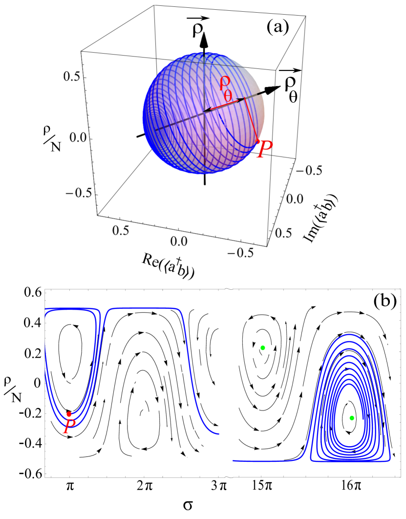
Figure 6: (a) Example of the dynamics in the pure Rabi regime ($\Lambda=0$) in a dissipative system. The orbit is an helix on the normalized Bloch sphere (Paria sphere), that starts from the point P set by the initial condition and tends toward a steady point on the $\rho_{\theta}$ axes, that remains well defined thanks to the normalization despite the steady state being the vacuum. Parameters are the same as in Fig. (1(h–i). (b) Projection of the dynamics on the $(\rho,\sigma)$ space, superimposed on the streamlines of the dynamical system. As compared to the Hamiltonian case, the fixed points (displayed as green points) are shifted. Starting from $\sigma_{0}=\pi$, the spiral gets farther from $\pi$, then drifts as the system enters in the running-phase regime, and ultimately gets absorbed by the fixed point near $16\pi$. The left spiral is unstable, while the right one is stable.

Now, in the cases where the $\vec{\rho}_{\theta}$ axis is not aligned with the observable $\vec{\rho}$ axis—which is all the cases except at resonance—and if the initial and final points on $\vec{\rho}_{\theta}$ are on opposite side of its zero, then the circle will come to encircle for some time the $\vec{\rho}$ axis, corresponding to the running regime of relative phase, until it drifts again on the other side of the sphere, at which point the system goes to the oscillatory regime. It can happen that this spiral will pass by the north or south pole of the $\vec{\rho}$ axis, which means that in the basis of observables, one population becomes exactly zero, leading to an undefined relative phase. This is not, however, compulsory. In other cases, depending on the interplay between decay and detuning, the trajectory remains the whole time on one side of the sphere, in which case the system is always in the oscillating-phase regime and there is no switching.

There are other notable behaviours that are conveniently pictured on the sphere. At resonance ($\delta=0$) and for dressed states ($\rho_{0}=\pm N/2$), when $\Gamma_{-}=0$, the relative phase starts at $\pi/2$ and is then locked at $\pm\pi/2$ forever. This is a manifestation of optimal strong-coupling with full-amplitude Rabi oscillations at the Rabi frequency. Moreover, the population imbalance oscillates in time around $\rho=0$ while decaying toward zero. Still at resonance, but now when $\Gamma_{-}\neq 0$, the relative phase oscillates in time taking all the values between $\pm\pi/2$ while the population imbalance decays faster as compared to the former case. Out of resonance, $\delta\neq 0$, when $\Gamma_{-}=0$ the relative phase exhibits the same trend as the Hamiltonian regime, however, the population decays in time.

IV.2 Classification of fixed points

The stability analysis in the Liouvillian case shows that the dynamics is richer and visits extended areas of the stability diagram. This results in the family of $\mathrm{L}$ points in Fig. 3 that we introduce and discuss individually below. This new phenomenology is an important consideration for polaritons that are inherently finite-lifetime particles.

The same stability treatment as before but now with the system of Eqs. (5) yields for $\tau$ and $\Delta$:

$$\tau= -4\Gamma_{-}\rho^{\ast}/N\,,$$ (23a)

$$\Delta= (4/(1-4(\rho^{*}/N)^{2}))-\Gamma_{-}^{2}(1-4(\rho^{*}/N)^{2}))\,.$$ (23b)

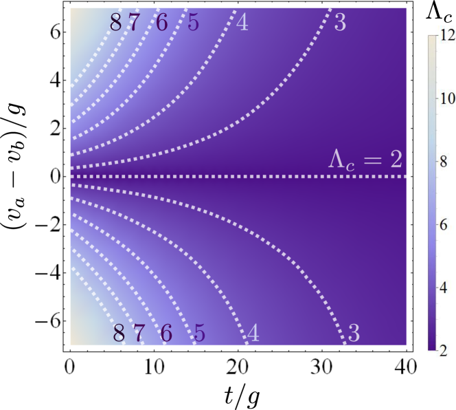
Figure 7: When the interactions of the two condensates are not equal, $v_{a}\neq v_{b}$, the critical $\Lambda_{c}$ becomes time-dependent, as shown here as a density plot for the case of zero detuning. The smallest value is $\Lambda_{c}=2$ which is the textbook value for the Josephson regime in the case of equal interactions, at resonance and without dissipation, as recovered here for this particular case. Variations result in an increase of $\Lambda_{c}$, that decays with time to tend towards this fundamental value.

This shows how $\Gamma_{-}\equiv\gamma_{b}-\gamma_{a}$ (as defined in Eq. (6) but here with $p_{a}=p_{b}=0$) defines new types of fixed points in the $\Delta>0$ region, namely, the system can also spiral towards its fixed points ($\mathrm{LUD}$ and $\mathrm{LID}_{(\Lambda\leq\Lambda_{c})}$ points), as expected from decay, instead of always orbiting them as before ($\mathrm{LUR}$ and $\mathrm{LIR}_{(\Lambda\leq\Lambda_{c})}$ points). An example of a $\mathrm{LUD}$ trajectory, i.e., in the non-interacting (Rabi) regime and in presence of detuning and decay, is given in Fig. 6.

From the layout of points in Fig. 3, the stability property of the fixed points in presence of decay thus remains a good criterion to set apart the Rabi and Josephson regimes. $\Lambda_{c}$ is still defined according to Eq. (20), but becomes time dependent when $v_{a}\neq v_{b}$ since in this case it depends through $\Delta E$—itself defined in Eq. (3a)—on the total population $N$ that decays according to $N(t)\approx N(0)\exp(-(\gamma_{a}+\gamma_{b})t/2)$ (the exact solution is more complex than this overall pattern; it typically oscillates around this envelope due to interactions and may exhibit complicated patterns with abrupt variations in some particular cases, with a dynamics that would deserve an analysis of its own). The dependence of $\Lambda_{c}$ as function of time and the detuning in interactions, $v_{a}-v_{b}$, is shown in Fig. 7 for the case of bare mode resonances, $\delta=0$, where it is seen that $v_{a}=v_{b}$ makes it time-independent indeed and pinned to the textbook value $\Lambda_{c}=2$, while an interaction imbalance results in a dependence of $\Lambda_{c}$ similar to that due to detuning (cf. Fig. 5). That is, the threshold for the Josephson regime is increased and decays in time down to the value $\Lambda_{c}$ of Eq. (20) at long times. The Rabi regime is therefore always recovered since also $\Lambda$, Eq. (3b), decays with time, proportionally to $N$. We now discuss the various fixed points in detail, starting with the non-interacting case ($v_{a}=v_{b}=0$) and then considering interactions. In both cases, however, note that with decay only (no pumping), the steady state is the vacuum, but is approached in a limit that is well-defined and that allows the following discussion. Even more enlighteningly, it can be seen as a fixed point on the normalized Bloch sphere, showing again the value of this ghost object of varying radius that unifies the dynamics of relative phase and population imbalance in a transparent way. To distinguish this variation of dynamically evolving sphere from the conventional Bloch sphere, we would propose a dedicated terminology and refer to it as a “Paria sphere” (after the American ghost city).

IV.2.1 Non-interacting case

In the dissipative Rabi regime, that is, with decay but no interactions, the fixed points are given by:

$$(\rho^{*})^{2} =\frac{N^{2}}{8\Gamma_{-}^{2}}[-4+\Gamma_{-}^{2}-\Delta E^{2}$$

$$+\sqrt{\Delta E^{4}+2\Delta E^{2}(4+\Gamma_{-}^{2})+(-4+\Gamma_{-}^{2})^{2}}]\,,$$ (24a)

$$\sin(\sigma^{*}) =\frac{1}{2}\Gamma_{-}\sqrt{1-4(\rho^{*}/N)^{2}}\,.$$ (24b)

Therefore, for zero detuning and $|\Gamma_{-}|\leq 2$, one finds the fixed points at $(\rho^{*}=0,\sigma^{*}=\sin^{-1}(\Gamma_{-}/2))$ and even in the dissipative regime, these fixed points remain centers ($\mathrm{LUR}_{|\Gamma_{-}|<2}$). Increasing $|\Gamma_{-}|$ makes two consecutive centers from the set of fixed points approach each other along the $\rho=0$ axis until they meet when $|\Gamma_{-}|=2$ with the common phase $\sigma=(2k+1)\pi/2$ for integer $k$, at which point they become degenerate, as the $\mathrm{LUR}_{(|\Gamma_{-}|=2)}$ points. For $|\Gamma_{-}|>2$, the fixed points split again but now along the $\sigma$ axis, as they keep a common value for the phase but depart in population imbalance according to $\rho^{*}=\pm\sqrt{(-4+\Gamma_{-}^{2})/4\Gamma_{-}^{2}}$. Past $|\Gamma_{-}|>2$, the fixed points also change their stability property to become spiral points ($\mathrm{LUR}_{(|\Gamma_{-}|>2)}$). Beside, they are now connected by streamlines in the $(\rho,\sigma)$ space, i.e., starting close from the unstable point brings the system towards the other point, that is stable. At non-zero detuning, the fixed points always are of the spiraling type, $\mathrm{LUD}$. Finally, it can be shown that the condition $\tau^{2}-4\Delta<0$ separating spirals from nodal points is always satisfied, so the system is at most spiraling.

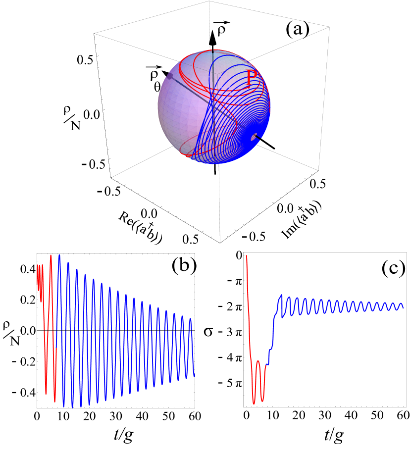
Figure 8: (a) Switching from the Josephson (red trace) to the Rabi (blue trace) regimes in an interacting, dissipative system. Here we set $va=vb$. P is the starting point in a system of the $\mathrm{LI}_{(\Lambda>\Lambda_{c})}$ type. Due to decay, the system eventually switches to the Rabi regime, with the dynamics ending at a point on the $\rho_{\theta}$ axes. (b) The population imbalance shows two kinds of self-trapping, one at early times (in red) that is induced by the interactions, the other at later times (in blue) that is induced by detuning. (c) The relative phase also exhibit a switching between the oscillating- and running-phases, in a way such that all the four possible combinations (Josephson–Running-phase; Josephson–Oscillating-phase; Rabi–Running-phase and Rabi–Oscillating-phase) happen in succession. Parameters: $\rho_{0}=0.3N$, $\sigma_{0}=0$, $\Delta E=0.5$, $\Lambda(0)=12$, $\gamma_{a}=0.25g$ and $\gamma_{b}=0.05g$.

IV.2.2 Interacting case

Clearly, with decay, the total number of particles decays with time, and even if starting in the Josephson regime, ultimately the system gets into the Rabi regime where tunneling (or coupling) dominates over interactions. That is, the system eventually follows the dynamics of Eqs. (5), that yields the steady state of the previous Section through Eqs. (24). Such a transition between the two regimes might in fact be the clearest evidence of the Josephson regime in a dissipative context. This is illustrated with the example of the dynamics in Fig. 8, that starts from a point in the Josephson regime, i.e., a $\mathrm{LI}_{(\Lambda>\Lambda_{c})}$ point in Fig. 3. Then $\Lambda$ decays along with the number of particles as time passes, and the helix drifts till $\Lambda=\Lambda_{c}$ at which point the dynamics switches to the Rabi regime (now plotted in Blue as compared to Red in the Josephson regime), and subsequently spirals along the $\rho_{\theta}$ axis. Such a switching gives rise to two kinds of “population trapping”, i.e., nonzero time-averaged population imbalance $\langle\rho\rangle$. One trapping is caused by the interactions, and occurs in the Josephson regime, while another type of trapping is caused instead merely by detuning, and occurs in the Rabi regime. Just as the distinction between the Rabi and the Josephson regimes might be arduous to make in cases where interactions, detuning and decay compete, also the type of trapping could be ambiguous. A decay-induced switching of regime is shown in Fig. 8(b), with two types of trapping on both sides of the switching. Figure 8(c) shows the behavior of the relative phase versus time, changing from running-phase to oscillatory as $\Lambda$ decays, up to the switching time, after which point the phase runs again but in the Rabi regime until, eventually, it is brought back to the oscillating-phase regime (still in the Rabi regime). With this example, one can see the diversity of the possible regimes, both for the dynamics of the relative phase (running and oscillatory) and for the type of the oscillations (Josephson and Rabi). While the interaction mediates the change of regime, decay mediates the change in the phase dynamics. In total, we have four combinations that succeed to each others, that illustrate well the complexity of the phenomenon when considered in its full generality.

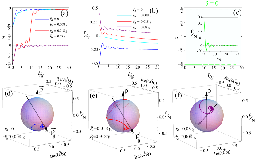
Figure 9: (a) Relative phase and (b) population imbalance in a dissipative system with pumping but in absence of interactions. Parameters: $\delta=1.5$ and $p_{b}=8\times 10^{-3}g$. The relative phase only display the oscillatory regime even though it can jump between fixed points. (c) Relative phase at resonance ($\delta=0$), in which case, for any pumping ratio, it is a two-valued sawtooth function. In this case, the population imbalance goes toward zero. (d–f) Dynamics on the Bloch sphere for the three different pumping ratio considered in panel (a). The trajectories never encircle the vertical $\vec{\rho}$ axis, thereby suppressing the running-regime of the phase. Parameters for all panels: $\gamma_{a}=0.2g$ and $\gamma_{b}=0.02g$.

V Pumping

V.1 Dynamics

We now succinctly consider the dynamics of relative phase from Eqs. 7 with nonzero $p_{a}$ and $p_{b}$, that is, in presence of incoherent pumping. The general case would bring us too far astray and we therefore limit our discussion to the pure Rabi regime (non-interacting case). We first consider the transient, starting from the vacuum and then briefly describe the steady state situation before giving it full attention in next section.

Starting from vacuum, the relative phase is ill-defined at $t=0$. With pumping, populations in both states increase and a relative phase is established. Note that while $S=0$ at all times since both $\langle a\rangle$ and $\langle b\rangle$ remain zero under incoherent pumping—that randomizes the phase of each mode—the cross-correlator $\sigma=\langle{a^{\dagger}}b\rangle$ is well defined and gets interconnected to particles tunneling in a way similar to the Hamiltonian case. This supports the idea that there is no absolute phase for the condensate but a degree of cross-coherence, or correlation, which, for the sake of convenience, we can still refer to as a relative phase (its argument, $\sigma$ is for all purposes a relative phase). This phase sets itself at the value $\pm\pi/2$ at early times depending on the ratio $p_{a}/p_{b}$. Figure 9(a-b) shows its subsequent evolution along with the population imbalance. When $p_{a}/p_{b}\leq 1$, the relative phase starts from $\approx\pi/2$ and then evolves oscillatory in time towards its steady value of $\approx\pi$. Meanwhile, the population imbalance remains negative while its absolute value increases. When $p_{a}/p_{b}>1$, the relative phase starts from $\approx-\pi/2$. Also, its time evolution is different than the case $p_{a}/p_{b}\leq 1$. As shown in Fig. 9(a-b) for $p_{a}=0.018g$, there are oscillations around zero followed by a jump to oscillations around $\pi$. This behavior is connected to the population imbalance that changes sign (from positive to negative), crossing zero. For the oscillations in the relative phase to end up with its steady state around $0$, the population imbalance must remain positive. At resonance ($\delta=0$), the relative phase remains $\pm\pi/2$ for any pumping ratio, and the population imbalance shows damped oscillations around zero. This is shown in Fig. 9(c).

Panels (d-f) of Fig. 9 shows the corresponding dynamics on the Bloch sphere for three pumping ratios. The trajectory in each case starts from the point close to the south or north pole of the observable axis, then drifts toward a steady point near the eigenstate axis. As can be seen in the figures, the trajectory is immediately brought from the observable axis to the eigenstate one, and thus has no chance to loop around or intersect the $\vec{\rho}$ axis. As a consequence, the relative phase only displays damped oscillations. Consequently, the running-phase regime is suppressed by incoherent pumping. Finally, we have considered non-interacting systems only but also a fairly simple model of pumping, through Lindblad operators that are the direct counterpart of spontaneous decay. Voronova et al. have reported interesting instabilities akin to Kapitza’s pendulum in driven interacting Rabi–Josephson systems with a more elaborate model of pumping (through a reservoir) arXiv_voronova16a , hinting the complexity of the more general cases.

V.2 Classification of fixed points

The stability analysis in presence of pumping brings some qualitative novelties due to the randomization of the phase. First, the fixed points now lie in a four-dimensional space instead of two before, since in the steady state the phase acquires a definite complex value, adding two dimensions and making obsolete the criterion of running vs oscillating phase on the Paria (normalized Bloch) sphere. Solving Eqs. (7) in the steady state (with $v_{a}=v_{b}=0$), one finds:

$$n^{*}=\begin{aligned} &[p_{a}(-4\Gamma_{+}+(\Gamma_{-}-\Gamma_{+})(\delta^{2}+\Gamma_{+}^{2}))\\ &-p_{b}(4\Gamma_{+}+(\Gamma_{-}+\Gamma_{+})(\delta^{2}+\Gamma_{+}^{2}))]/Y\,,\end{aligned}$$ (25a)

$$\rho^{*}=[(\delta^{2}+\Gamma_{+}^{2})(\Gamma_{+}(p_{b}-p_{a})+\Gamma_{-}(p_{a}+p_{b})]/2Y\,,$$ (25b)

$$\mathrm{Re}[\langle a^{\dagger}b\rangle^{*}]=-\delta(\Gamma_{+}(p_{b}-p_{a})+\Gamma_{-}(p_{a}+p_{b}))/Y\,,$$ (25c)

$$\mathrm{Im}[\langle a^{\dagger}b\rangle^{*}]=-(\Gamma_{+}/\delta)\mathrm{Re}[\langle a^{\dagger}b\rangle^{*}]\,,$$ (25d)

where $Y$ stands for $(\Gamma_{-}^{2}-\Gamma_{+}^{2})(\delta^{2}+\Gamma_{+}^{2})-4\Gamma_{+}^{2}$. Note that Eqs. (25c–25d) are more simply expressed as $\sigma^{*}=\arctan(-\Gamma_{+}/\delta)$. While the dimension of the space is larger, there is however a single fixed point, due to the unicity of the steady state solution. The stability of this point follows from the eigenvalues of the Jacobian matrix, these being:

$$\lambda_{pq}=\Gamma_{+}+pi\sqrt{qX+\sqrt{X^{2}+4\Gamma_{-}^{2}\delta^{2}}}\,,$$ (26)

where $X\equiv\Gamma_{-}^{2}-\delta^{2}-4$ and where $p$ and $q$ take the values $\pm 1$ (we label them with the sign only, so that, e.g., $\lambda_{+-}=\Gamma_{+}+i\sqrt{-X+\sqrt{X^{2}+4\Gamma_{-}^{2}\delta^{2}}}$). The corresponding eigenvectors $v_{pq}$ provide the directions in the $(\rho,n,\sigma)$ four-dimensional space along which the system flows when slightly perturbed. There is no obvious geometrical features to characterize $v_{pq}$. The stability properties are the following: if $\Gamma_{+}<0$ and $Y<0$, the fixed point is stable. If only $\Gamma_{+}<0$ is satisfied, the subspace spanned by $\left\{v_{--},v_{-+},v_{+-}\right\}$ is stable while any combination involving $v_{++}$ is unstable. On the contrary, if only $Y<0$ is satisfied, the only stable subspace is spanned by $v_{++}$ while any other possible linear superposition yields an unstable point. For $\Gamma_{+}>0$, the dynamics is generally unstable, and, interestingly, can feature saddle-type of instability, that in the Hamiltonian or dissipative regime (without pumping), was used as a criterion for the Josephson regime, where the dynamics is ruled by the (weak) interactions. Here the system has no interactions, but can still manifest this type of saddle instability and in different ways, for instance when the condition $\Gamma_{+}>0$ and $Y<0$ is met. The presence of a saddle-type of instability in a non-interacting system may be disconcerting, because this served in the previous cases as a robust criterion to identify the Josephson regime, so arguably doubts may arise on what precisely defines the Josephson regime in the most general situation. One could then look for a deeper characterization to establish such a general criterion when also including pumping, for instance, through the number of fixed points, or one could also upgrade the Josephson regime to the realm of pumping non-interacting systems. However, these various approaches, although they match the facts, lack a clear physical motivation, so we leave it an open question whether a general definition is suitable in the most general case that combines pumping, decay, detuning and interactions. Another case worthy of interest is $\Gamma_{+}=0$ and $Y=0$, that results in pure imaginary eigenvalues. This gives rise to a center subspace, that results in a type of bifurcation known as a “transcritical bifurcation” strogatz_book94a , that is, the fixed point exchanges its stability when passing by $\Gamma_{+}=0$ or $Y=0$.

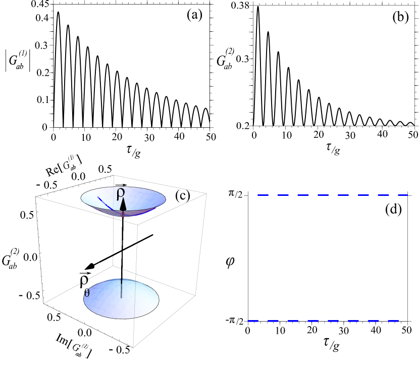
Figure 10: (a–b) $\tau$–Dynamics of the two-time correlators $G^{(1)}_{ab}$ and $G^{(2)}_{ab}$ in the steady state of a dissipative system at resonance and without interactions. (c) In autocorrelation time, rather than a sphere, the trajectory lies on the upper sheet of an hyperboloid. A red point indicates the starting point. (d) Phase of $G^{(1)}_{ab}$, in the oscillating-regime.

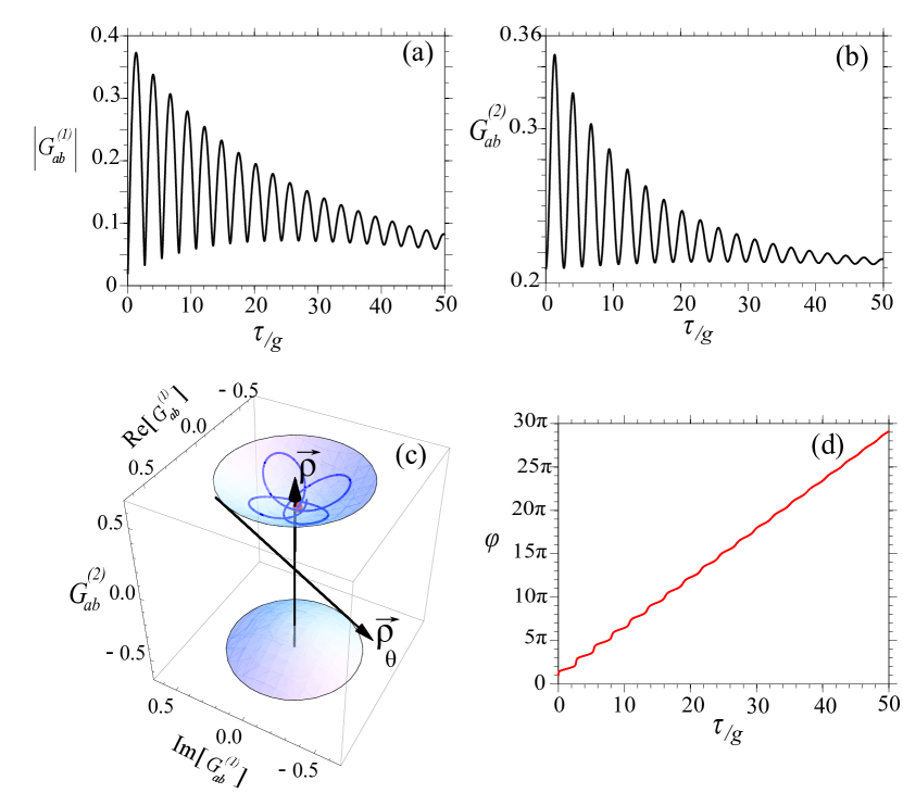
Figure 11: Courresponding $\tau$–Dynamics of $G^{(1)}_{ab}$ and $G^{(2)}_{ab}$ of Fig. 10 but in a detuned system. (c) The dynamics on the hyperboloid is now open and as a result, (d), the the phase of $G^{(1)}_{ab}$ is in the running-regime.

V.3 Dynamics in autocorrelations

We have clarified the dynamics in real time thanks to a normalized Bloch sphere, and articulated the fundamental links between the phase and population imbalance in both pure Hamiltonian dynamics and in the transient dynamics of a driven dissipative system. In this section, we explore possible similar relationships in a steady state situation, where the $t$ dynamics has converged to constant values by definition, with only dynamics in the correlations remaining. The natural operators to consider are:

$$G^{(1)}_{ab}(\tau) =\lim_{t\rightarrow\infty}\langle a^{\dagger}(t+\tau)b(\tau)\rangle\,,$$ (27a)

$$G^{(2)}_{ab}(\tau) =\lim_{t\rightarrow\infty}\langle a^{\dagger}(t)b^{\dagger}(\tau+t)b(\tau+t)a(t)\rangle\,.$$ (27b)

The former, the crossed first order correlation function $G^{1}_{ab}(\tau)$, is related to coherence between the states and suggests as an extension for steady states of $\sigma$, the relative phase in autocorrelation time $\varphi\equiv\arg(G^{(1)}_{ab})$. The latter is related to fluctuations of the population imbalance in autocorrelation time. Correspondingly, the question pauses itself whether these two observables are geometrically connected or not. Using Eqs. (7) and the quantum regression theorem, the following relationship can be obtained:

$$G^{(1)}_{ab}(\tau)=\lim_{t\rightarrow\infty}\frac{1}{\omega}\exp((\delta+i\Gamma_{+})\tau/2)\\ \big{[}\langle a^{\dagger}(t)b(t)\rangle(\omega\cos(\omega\tau/2)+(i\delta+\Gamma_{-})\sin(\omega\tau/2))\\ -2i\langle a^{\dagger}(t)a(t)\rangle\sin(\omega\tau/2)\big{]}\,,$$ (28)

where we have introduced a complex frequency $\omega=\sqrt{4+(\delta-i\Gamma_{-})^{2}}$. By also writing the equation of motion for $G^{(2)}_{ab}(\tau)$, it can be shown that Eqs. (27) are related through the relation:

$$G^{(2)}_{ab}(\tau)=|G_{ab}^{(1)}(\tau)|^{2}+\lim_{t\rightarrow\infty}\frac{N^{2}}{4}\,.$$ (29)

This shows that $G^{(1)}_{ab}$ and $G^{(2)}_{ab}$ are coupled indeed, with a possible similar Josephson interpretation that one is driving the other. However, their connection is through a two-sheet hyperboloid and is thus completely different than the the dynamics of real-time observables, even for the transient dynamics, where variables are connected via a sphere of variable radius (the Paria sphere).

Figure 10 shows the trajectory in the hyperboloid at resonance ($\delta=0$). In this case, the relative phase is a two-valued function, oscillating between $\pm\pi/2$ (Fig. 10 (d)), which corresponds to the the oscillatory regime of the relative phase. Correspondingly, $G^{(1)}_{ab}$ and $G^{(2)}_{ab}$ oscillate in time with a decay toward zero for $G^{(1)}_{ab}$ and $N^{2}/4$ for $G^{(2)}_{ab}$. Comparing with panel (d), it is observed that $\varphi$ changes value whenever $G^{(1)}_{ab}$ becomes zero. This shows a similar behaviour than in the real-time behaviour where whenever the relative phase becomes ill-defined due to one state becomings zero avoid, it changes its regime. Here, ill-defined coherence changes the value of phase instead. Simultaneously, $G^{(2)}_{ab}$ reaches $N^{2}/4$, which is the point of lowest possible fluctuations. The corresponding trajectory on the hyperboloid in panel (c) shows a simple line (in the curved space) with $\mathrm{Re}[G^{(1)}_{ab}]=0$ and $G^{(2)}_{ab}$ swinging around the lowest point of the hyperboloid. The detuned case ($\delta\neq 0$) is shown in Fig. 11. This time, as seen in panel (d), the relative phase is running. Both $G^{(1)}_{ab}$ and $G^{(2)}_{ab}$ oscillate and decay toward different steady points as compared to resonance. The trajectory on the hyperboloid shows this time an open orbit, encircling the hyperboloid $G^{(2)}_{ab}$ axis without ever touching it. In contrast to the real-time dynamics on the Paria sphere, in autocorrelation time, there is a reduced phenomenology and, in particular, no preferred change of basis, e.g., there is no counterpart of a regime of drifting phase out of resonance and two-valued $\pm\pi/2$ phase at resonance. This is due to the Hamiltonian dynamics being washed out by the incoherent pumping.

VI Conclusions

In conclusion, we have generalized and unified the problem of Rabi and Josephson oscillations between two weakly interacting condensates to include i) detuning, ii) different interactions for each condensate and iii) decay. We have also overviewed the situation with pumping, which, however, requires a dedicated analysis of its own. Our results show that even at the simplest mean-field level, such a fundamental problem had kept some fundamental features hidden through the particular cases that had been focused on so far. For instance, the relative phase $\sigma$ and population imbalance $\rho$ appear in the most general case as two sides of the same coin without one driving the other, and their qualitative behaviour depends on a choice of representation, with a basis that can always be chosen in which there is a linear phase drift in the pure Rabi regime. At such, the behaviour of the relative phase can not be associated to neither the Josephson nor the Rabi regime exclusively, although it bears some degree of correlation with it, and is instead a topological feature. Similar restrains apply to self-trapping. Such relationships are elegantly captured on a Bloch sphere of varying radius (that we termed Paria sphere) that clarifies an otherwise perplexing dynamics such as a shift of the regime of relative-phase from oscillating to running and oscillating again. An unambiguous general criterion to identify the Rabi ($\Lambda<\Lambda_{c}$) and Josephson ($\Lambda>\Lambda_{c}$) regimes has been provided through the critical effective interaction $\Lambda_{c}$, Eq. (20), that generalizes the case found in the literature at resonance and for equal interactions, in which case $\Lambda_{c}=2$. In the Hamiltonian case, when $\Lambda<\Lambda_{c}$, there are two fixed points that are centers for the dynamics. When $\Lambda>\Lambda_{c}$, there four fixed points, the one at $\sigma=0$ and lying between the two other fixed points being a saddle point, with all other points being centers. Similar analyses have been undertaken in the Liouvillian case and are summarized in Fig. 3. Since in this case the number of particles dies in time, the system always eventually shifts to the Rabi regime. In the case of different interaction strengths, also the critical $\Lambda_{c}$ becomes time dependent. Rather than the observation of mere oscillations and/or population trapping, a clear identification of the Josephson regime in finite-lifetime particles can instead be made by observing the transition in time from one regime to the other.

- (1) Landau, L. & Ginzburg, V. On the theory of superconductivity. Zh. Eksp. Teor. Fiz 20, 1964 (1950).
- (2) Josephson, B. Possible new effects in superconductive tunnelling. Phys. Lett. 1, 251 (1962).
- (3) Anderson, P. W. & Rowell, J. M. Probable observation of the Josephson superconducting tunneling effect. Phys. Rev. Lett. 10, 230 (1963).
- (4) Javanainen, J. Oscillatory exchange of atoms between traps containing bose condensates. Phys. Rev. Lett. 57, 3164 (1986).
- (5) Anderson, P. W. Considerations on the flow of superfluid helium. Rev. Mod. Phys. 38, 298 (1966).
- (6) Varoquaux, E. Anderson’s considerations on the flow of superfluid helium: Some offshoots. Rev. Mod. Phys. 87, 803 (2015).
- (7) Leggett, A. J. & Sols, F. On the concept of spontaneously broken gauge symmetry in condensed matter physics. Found. Phys. 21, 353 (1991).
- (8) Castin, Y. & Dalibard, J. Relative phase of two Bose-Einstein condensates. Phys. Rev. A 55, 4330 (1997).
- (9) Molmer, K. Optical coherence: A convenient fiction. Phys. Rev. A 55, 3195 (1997).
- (10) Antón, C. et al. Operation speed of polariton condensate switches gated by excitons. Phys. Rev. B 89, 235312 (2014).
- (11) Javanainen, J. & Rajapakse, R. Bayesian inference to characterize Josephson oscillations in a double-well trap. Phys. Rev. A 92, 023613 (2015).
- (12) Leggett, A. J. Bose-Einstein condensation in the alkali gases: Some fundamental concepts. Rev. Mod. Phys. 73, 307 (2001).
- (13) Leggett, A. J. BEC: The alkali gases from the perspective of research on liquid helium. AIP Conf. Proc. 477, 154 (1999).
- (14) Veksler, H. & Fishman, S. Semiclassical analysis of Bose—Hubbard dynamics. New J. Phys. 17, 053030 (2015).
- (15) Barone, A. & Paterno, G. Physics and application of the Josephson Effect (Wiley, New York, 1982).
- (16) Jaklevic, R. C., Lambe, J., Silver, A. H. & Mercereau, J. E. Quantum interference effects in Josephson tunneling. Phys. Rev. Lett. 12, 159 (1964).
- (17) Kleiner, R., Koelle, D., Ludwig, F. & Clarke, J. Superconducting quantum interference devices: State of the art and applications. Proc. IEEE 92, 1534 (2004).
- (18) McDonald, D. G. The nobel laureate versus the graduate student. Physics Today 54, 46 (2001).
- (19) Gati, R. & Oberthaler, M. K. A bosonic Josephson junction. J. Phys. B.: At. Mol. Phys. 40, R61 (2007).
- (20) Pereverzev, S. V., Loshak, A., Backhaus, S., Davis, J. C. & Packard, R. E. Quantum oscillations between two weakly coupled reservoirs of superfluid 3He. Nature 388, 449 (1997).
- (21) Albiez, M. et al. Direct observation of tunneling and nonlinear self-trapping in a single bosonic josephson junction. Phys. Rev. Lett. 95, 010402 (2005).
- (22) Kavokin, A., Baumberg, J. J., Malpuech, G. & Laussy, F. P. Microcavities (Oxford University Press, 2011), 2 edn.
- (23) Kasprzak, J. et al. Bose–Einstein condensation of exciton polaritons. Nature 443, 409 (2006).
- (24) Amo, A. et al. Collective fluid dynamics of a polariton condensate in a semiconductor microcavity. Nature 457, 291 (2009).
- (25) Sarchi, D., Carusotto, I., Wouters, M. & Savona, V. Coherent dynamics and parametric instabilities of microcavity polaritons in double-well systems. Phys. Rev. B 77, 125324 (2008).
- (26) Wouters, M. Synchronized and desynchronized phases of coupled nonequilibrium exciton-polariton condensates. Phys. Rev. B 77, 121302(R) (2008).
- (27) Shelykh, I. A., Solnyshkov, D. D., Pavlovic, G. & Malpuech, G. Josephson effects in condensates of excitons and exciton polaritons. Phys. Rev. B 78, 041302(R) (2008).
- (28) Lagoudakis, K. G., Pietka, B., Wouters, M., André, R. & Deveaud-Plédran, B. Coherent oscillations in an exciton-polariton Josephson junction. Phys. Rev. Lett. 105, 120403 (2010).
- (29) Abbarchi, M. et al. Macroscopic quantum self-trapping and josephson oscillations of exciton polaritons. Nat. Phys. 9, 275 (2013).
- (30) Aleiner, I. L., Altshuler, B. L. & Rubo, Y. G. Radiative coupling and weak lasing of exciton-polariton condensates. Phys. Rev. B 85, 121031(R) (2012).
- (31) Pavlovic, G., Malpuech, G. & Shelykh, I. A. Pseudospin dynamics in multimode polaritonic Josephson junctions. Phys. Rev. B 87, 125307 (2013).
- (32) Khripkov, C., Piermarocchi, C. & Vardi, A. Dynamics of microcavity exciton polaritons in a josephson double dimer. Phys. Rev. B 88, 235305 (2013).
- (33) Racine, D. & Eastham, P. R. Quantum theory of multimode polariton condensation. Phys. Rev. B 90, 085308 (2014).
- (34) Gavrilov, S. S. et al. Nonlinear route to intrinsic josephson oscillations in spinor cavity-polariton condensates. Phys. Rev. B 90, 235309 (2014).
- (35) Zhang, C. & Zhang, W. Exciton-polariton Josephson interferometer in a semiconductor microcavity. Europhys. Lett. 108, 27002 (2014).
- (36) Ma, X., Chestnov, I. Y., Charukhchyan, M. V., Alodjants, A. P. & Egorov, O. A. Oscillatory dynamics of nonequilibrium dissipative exciton-polariton condensates in weak-contrast lattices. Phys. Rev. B 91, 214301 (2015).
- (37) Rayanov, K., Altshuler, B., Rubo, Y. & Flach, S. Frequency combs with weakly lasing exciton-polariton condensates. Phys. Rev. Lett. 114, 193901 (2015).
- (38) Zhang, L. et al. Weak lasing in one-dimensional polariton superlattices. Proc. Natl. Acad. Sci. 112, E1516 (2015).
- (39) Voronova, N. S., Elistratov, A. A. & Lozovik, Y. E. Detuning-controlled internal oscillations in an exciton-polariton condensate. Phys. Rev. Lett. 115, 186402 (2015).
- (40) Dominici, L. et al. Ultrafast control and Rabi oscillations of polaritons. Phys. Rev. Lett. 113, 226401 (2014).
- (41) Agarwal, G. S. & Puri, R. R. Exact quantum-electrodynamics results for scattering, emission, and absorption from a Rydberg atom in a cavity with arbitrary Q. Phys. Rev. A 33, 1757 (1986).
- (42) Carmichael, H. J., Brecha, R. J., Raizen, M. G., Kimble, H. J. & Rice, P. R. Subnatural linewidth averaging for coupled atomic and cavity-mode oscillators. Phys. Rev. A 40, 5516 (1989).
- (43) Laussy, F. P., del Valle, E. & Tejedor, C. Luminescence spectra of quantum dots in microcavities. I. Bosons. Phys. Rev. B 79, 235325 (2009).
- (44) Liew, T., Rubo, Y. & Kavokin, A. Exciton-polariton oscillations in real space. Phys. Rev. A 90, 245309 (2014).
- (45) Colas, D. & Laussy, F. Self-interfering wave packets. Phys. Rev. Lett. 116, 026401 (2016).
- (46) Raghavan, S., Smerzi, A., Fantoni, S. & Shenoy, S. R. Coherent oscillations between two weakly coupled Bose–Einstein condensates: Josephson effects, oscillations, and macroscopic quantum self-trapping. Phys. Rev. A 59, 620 (1999).
- (47) Marino, I., Raghavan, S., Fantoni, S., Shenoy, S. R. & Smerzi, A. Bose-condensate tunneling dynamics: Momentum-shortened pendulum with damping. Phys. Rev. A 60, 487 (1999).
- (48) Sakmann, K., Streltsov, A. I., Alon, O. E. & Cederbaum, L. S. Exact quantum dynamics of a Bosonic Josephson Junction. Phys. Rev. Lett. 103, 220601 (2009).
- (49) Chuchem, M. et al. Quantum dynamics in the bosonic Josephson junction. Phys. Rev. A 82, 053617 (2010).
- (50) Agarwal, G. S. Vacuum-field Rabi splittings in microwave absorption by Rydberg atoms in a cavity. Phys. Rev. Lett. 53, 1732 (1984).
- (51) Carmichael, H. J. Statistical methods in quantum optics 1 (Springer, 2002), 2 edn.
- (52) del Valle, E. Microcavity Quantum Electrodynamics (VDM Verlag, 2010).
- (53) Zibold, T., Nicklas, E., Gross, C. & Oberthaler, M. K. Classical bifurcation at the transition from rabi to josephson dynamics. Phys. Rev. Lett. 105, 204101 (2010).
- (54) Voronova, N. S., Elistratov, A. A. & Lozovik, Y. E. Inverted pendulum state of a polariton Rabi oscillator. arXiv:1602.01457 (2016).
- (55) Rahmani, A. & Laussy, F. Rabi and Josephson oscillations. Wolfram Demonstration Project at http://demonstrations.wolfram.com/RabiAndJosephsonOscillations (2016).
- (56) Strogatz, S. H. Nonlinear Dynamics and Chaos (Perseus Books, 1994).