Document Neural Autoregressive Distribution Estimation

Abstract

We present an approach based on feed-forward neural networks for learning the distribution of textual documents. This approach is inspired by the Neural Autoregressive Distribution Estimator (NADE) model, which has been shown to be a good estimator of the distribution of discrete-valued high-dimensional vectors. In this paper, we present how NADE can successfully be adapted to the case of textual data, retaining from NADE the property that sampling or computing the probability of observations can be done exactly and efficiently. The approach can also be used to learn deep representations of documents that are competitive to those learned by the alternative topic modeling approaches. Finally, we describe how the approach can be combined with a regular neural network N-gram model and substantially improve its performance, by making its learned representation sensitive to the larger, document-specific context.

Keywords: Neural networks, Deep learning, Topic models, Language models, Autoregressive models

1 Introduction

One of the most common problem addressed by machine learning is estimating the distribution $p({\bf v})$ of multidimensional data from a set of examples $\{{\bf v}^{(t)}\}_{t=1}^{T}$. Indeed, good estimates for $p({\bf v})$ implicitly requires modeling the dependencies between the variables in ${\bf v}$, which is required to extract meaningful representations of this data or make predictions about this data.

The biggest challenge one faces in distribution estimation is the well-known curse of dimensionality. In fact, this issue is particularly important in distribution estimation, even more so than in other machine learning problems. This is because a good distribution estimator effectively requires providing an accurate value for $p({\bf v})$ for any value of $\bf v$ (i.e. not only for likely values of $\bf v$), with the number of possible values taken by $\bf v$ growing exponentially as the number of the dimensions of the input vector $\bf v$ increases.

One example of a model that has been successful at tackling the curse of dimensionality is the restricted Boltzmann machine (RBM) (Hinton, 2002). The RBM and other models derived from it (e.g. the Replicated Softmax of Salakhutdinov and Hinton (2009)) are frequently trained as models of the probability distribution of high-dimensional observations and then used as feature extractors. Unfortunately, one problem with these models is that for moderately large models, calculating their estimate of $p({\bf v})$ is intractable. Indeed, this calculation requires computing the so-called partition function, which normalizes the model distribution. The consequences of this property of the RBM are that approximations must be taken to train it by maximum likelihood and its estimation of $p({\bf v})$ cannot be entirely trusted.

In an attempt to tackle these issues of the RBM, the Neural Autoregressive Distribution Estimator (NADE) was introduced by Larochelle and Murray (2011). NADE’s parametrization is inspired by the RBM, but uses feed-forward neural networks and the framework of autoregression for modeling the probability distribution of binary variables in high-dimensional vectors. Importantly, computing the probability of an observation under NADE can be done exactly and efficiently.

In this paper, we describe a variety of ways to extend NADE to model data from text documents. We start by describing Document NADE (DocNADE), a single hidden layer feed-forward neural network model for bag-of-words observations, i.e. orderless sets of words. This requires adapting NADE to vector observations $\bf v$, where each of element $v_{i}$ represents a word and where the order of the dimensions is random. Each word is represented with a lower-dimensional, real-valued embedding vector, where similar words should have similar embeddings. This is in line with much of the recent work on using feed-forward neural network models to learn word vector embeddings (Bengio et al., 2003; Mnih and Hinton, 2007, 2009; Tomas Mikolov, 2013) to counteract the curse of dimensionality. However, in DocNADE, the word representations are trained to reflect the topics (i.e. semantics) of documents only, as opposed to their syntactical properties, due to the orderless nature of bags-of-words.

Then, we describe how to train deep versions of DocNADE. First described by Zheng et al. (2015) in the context of image modeling, here we empirically evaluate them for text documents and show that they are competitive to alternative topic models, both in terms of perplexity and document retrieval performances.

Finally, we present how the topic-level modeling ability of DocNADE can be used to obtain a useful representation of context for language modeling. We empirically demonstrate that by learning a topical representation of previous sentences, we can improve the perplexity performance of an N-gram neural language model.

2 Document NADE (DocNADE)

DocNADE is derived from the Neural Autoregressive Distribution Estimation (NADE) that will be first described in this section. Implemented as a feed-forward architecture, it extends NADE to provide an efficient and meaningful generative model of document bags-of-words.

2.1 Neural Autoregressive Distribution Estimation (NADE)

NADE, introduced in Larochelle and Murray (2011), is a tractable distribution estimator for modeling the distribution of high-dimensional vectors of binary variables. Let us consider a binary vector of $D$ observations, ${\bf v}\in\{0,1\}^{D}$. The NADE model estimates the probability of this vector by applying the probability chain rule as follows:

$$p({\bf v})=\prod_{i=1}^{D}p(v_{i}|{\bf v}_{<i}),$$ (1)

where $v_{i}$ denotes the $i$-th component of ${\bf v}$ and ${\bf v}_{<i}\in\{0,1\}^{i-1}$ contains the first $i-1$ components of ${\bf v}$: ${\bf v}_{<i}$ is the sub-vector $[v_{1},\dots,v_{i-1}]^{\top}$. The peculiarity of NADE lies in the neural architecture designed to estimate the conditional probabilities involved in Equation 1. To predict the component $i$, the model first computes its hidden layer of dimension $H$

$${\bf h}_{i}({\bf v}_{<i})={\bf g}\left({\bf c}+{\bf W}_{:,<i}{\bf v}_{<i}\right),$$ (2)

leading to the following probability model:

$$p(v_{i}=1|{\bf v}_{<i})=\mathrm{sigm}\left(b_{i}+{\bf V}_{i,:}{\bf h}_{i}({\bf v}_{<i})\right).$$ (3)

In these two equations, $\mathrm{sigm}(x)=1/(1+\exp(-x))$ denotes the sigmoid activation function while function ${\bf g}(\cdot)$ could be any activation function, though Larochelle and Murray (2011) also used the sigmoid function. ${\bf W}\in\mathbb{R}^{H\times D}$ and ${\bf V}\in\mathbb{R}^{D\times H}$ are the parameter matrices along with the associated bias terms ${\bf b}\in\mathbb{R}^{D}$ and ${\bf c}\in\mathbb{R}^{H}$, with ${\bf W}_{:,<i}$ being a matrix made of the $i-1$ first columns of ${\bf W}$.

Instead of a single projection of the input vector, the NADE model relies on a set of separate hidden layers ${\bf h}_{i}({\bf v}_{<i})$ that each represent the previous inputs in a latent space. The connections between input dimension $v_{i}$ and each hidden layer ${\bf h}_{i}({\bf v}_{<i})$ are tied as shown in figure 1, allowing the model to compute all the hidden layers for one input in $O(DH)$. The parameters $\{{\bf b},{\bf c},{\bf W},{\bf V}\}$ are learned by minimizing the average negative log-likelihood using stochastic gradient descent.

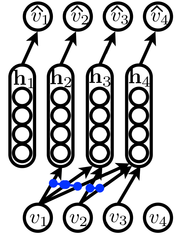
Figure 1: Illustration of NADE. Colored lines identify the connections that share parameters and $\widehat{v}_{i}$ is a shorthand for the autoregressive conditional $p(v_{i}|{\bf v}_{<i})$. The observations $v_{i}$ are binary.

2.2 From NADE to DocNADE

The Document NADE model (DocNADE) aims at learning meaningful representations of texts from an unlabeled collection of documents. This model embeds, like NADE, a set of hidden layers. Their role is to capture salient statistical patterns in the co-occurrence of words within documents and can be considered as modeling hidden topics.

To represent a document, the vector ${\bf v}$ is now a sequence of arbitrary size $D$. Each element of ${\bf v}$ corresponds to a multinomial observation over a fixed vocabulary of size $V$. Therefore $v_{i}\in\{1,...,V\}$ represents the index in the vocabulary of the $i$-th word of the document. For now, we’ll assume that an ordering for the words is given, but we will discuss the general case of orderless bags-of-words in Section 2.3.

The main approach taken by DocNADE is similar to NADE, but differs significantly in the design of parameter tying. The probability of a document ${\bf v}$ is estimated using the probability chain rule, but the architecture is modified to cope with large vocabularies. Each word observation $v_{i}$ of the document ${\bf v}$ leads to a hidden layer ${\bf h}_{i}$, which represents the past observations ${\bf v}_{<i}$. This hidden layer is computed as follows:

$${\bf h}_{i}({\bf v}_{<i})={\bf g}\left({\bf c}+\sum_{k<i}{\bf W}_{:,v_{k}}\right),$$ (4)

where each column of the matrix ${\bf W}$ acts as a vector of size $H$ that represents a word. The embedding of the $i^{th}$ word in the document is thus the column of index $v_{i}$ in the matrix ${\bf W}$.

Notice that by sharing the word representation matrix across positions in the document, each hidden layer $hh_{i}({\bf v}_{<i})$ is in fact independent of the order of the words within ${\bf v}_{<i}$. The implications of this choice is that the learned hidden representation will not model the syntactic structure of the documents and focus on its document-level semantics, i.e. its topics.

It is also worth noticing that we can compute ${\bf h}_{i+1}$ recursively by keeping track of the pre-activation of the previous hidden layer ${\bf h}_{i}$ as follows:

$${\bf h}_{i+1}({\bf v}_{<i+1})={\bf g}\left({\bf W}_{:,v_{i}}+\underbrace{{\bf c}+\sum_{k<i}{\bf W}_{:,v_{k}}}_{\text{Precomputed for}~{}{\bf h}_{i}({\bf v}_{<i})}\right)$$ (5)

The weight sharing between hidden layers enables us to compute all hidden layers ${\bf h}_{i}({\bf v}_{<i})$ for a document in $O(DH)$.

Then, to compute the probability of a full document $p({\bf v})$, we need to estimate all conditional probabilities $p(v_{i}|{\bf v}_{<i})$. A straightforward solution would be to compute each $p(v_{i}|{\bf v}_{<i})$ using softmax layers with a shared weight matrix and bias, each fed with the corresponding hidden layer ${\bf h}_{i}$. However, the computational cost of this approach is prohibitive, since it scales linearly with the vocabulary size.To overcome this issue, we represent distribution over the vocabulary by a probabilistic binary tree, where the leaves correspond to the words. This approach is widely used in the field of neural probabilistic language models (Morin and Bengio, 2005; Mnih and Hinton, 2009). Each word is represented by a path in the tree, going from the root to the leaf associated to that word. A binary logistic regression unit is associated to each node in the tree and gives the probability of the binary choice, going left or right. Therefore, a word probability can be estimated by the path’s probability in this tree, resulting in a complexity in $O(\log V)$ for trees that are balanced. In our experiments, we used a randomly generated full binary tree with $V$ leaves, each assigned to a unique word of the vocabulary. An even better option would be to derive the tree using Hoffman coding, which would reduce even more the average path lengths.

More formally, let’s denote by ${\bf l}(v_{i})$ the sequence of nodes composing the path, from the root of the tree to the leaf corresponding to word $v_{i}$. Then, ${\bm{\pi}}(v_{i})$ is the sequence of left/right decisions of the nodes in ${\bf l}(v_{i})$. For example, the root of the tree is always the first element $l(v_{i})_{1}$ and the value $\pi(v_{i})_{1}$ will be 0 if the word is in the left sub-tree and 1 if it is in the right sub-tree. The matrix $\bf V$ stores by row the weights associated to each logistic classifier. There is one logistic classifier per node in the tree. Let ${\bf V}_{l(v_{i})_{m},:}$ and $b_{l(v_{i})_{m}}$ be the weights and bias for the logistic unit associated to the node $n(v_{i})_{m}$. The probability $p(v_{i}|{\bf v}_{<i})$ given the tree and the hidden layer ${\bf h}_{i}({\bf v}_{<i})$ is computed with the following formulas:

$$p(v_{i}=w|{\bf v}_{<i})=\prod_{m=1}^{|{\bm{\pi}}(v_{i})|}p(\pi(v_{i})_{m}|{\bf v}_{<i}),\textrm{ with}$$ (6)

$$p(\pi(v_{i})_{m}=1|{\bf v}_{<i})=\mathrm{sigm}\left(b_{l(v_{i})_{m}}+{\bf V}_{l(v_{i})_{m},:}{\bf h}_{i}({\bf v}_{<i})\right).$$ (7)

This hierarchical architecture allows us to efficiently compute the probability for each word in a document and therefore the probability of every documents with the probability chain rules (see Equation 1). As in the NADE model, the parameters of the model $\{{\bf b},{\bf c},{\bf W},{\bf V}\}$ are learnt by minimizing the negative log-likelihood using stochastic gradient descent.

Figure 2: Illustration of DocNADE. Connections between each multinomial observation $v_{i}$ and hidden units are also shared, and each conditional $p(v_{i}|{\bf v}_{<i})$ is decomposed into a tree of binary logistic regressions.

Since there is $\log(V)$ logistic regression units for a word (one per node), each of them has a time complexity of $O(H)$, the complexity of computing the probability for a document of $D$ words is in $O(\log(V)DH)$.

As for using DocNADE to extract features from a complete document, we propose to use

$${\bf h}({\bf v})={\bf h}_{D+1}({\bf v}_{<D+1})={\bf g}\left({\bf c}+\sum_{k=1}^{D}{\bf W}_{:,v_{k}}\right)$$ (8)

which would be the hidden layer computed to obtain the conditional probability of a $D+1^{\rm th}$ word appearing in the document.

2.3 Training from bag-of-word counts

So far, we have assumed that the ordering of the words in the document is known. However, document datasets often take the form of word-count vectors in which the original word order, required to specify the sequence of conditionals $p(v_{i}|{\bf v}_{<i})$, has been lost.

Thankfully, it is still possible to successfully train DocNADE despite the absence of this information. The idea is to assume that each observed document ${\bf v}$ was generated by initially sampling a seed document $\widetilde{{\bf v}}$ from DocNADE, whose words were then shuffled using a randomly generated ordering to produce ${\bf v}$. With this approach, we can express the probability distribution of ${\bf v}$ by computing the marginal over all possible seed document:

$$p({\bf v})=\sum_{\widetilde{{\bf v}}\in{\cal V}({\bf v})}p({\bf v},\widetilde{{\bf v}})=\sum_{\widetilde{{\bf v}}\in{\cal V}({\bf v})}p({\bf v}|\widetilde{{\bf v}})p(\widetilde{{\bf v}})$$ (9)

where $p(\widetilde{{\bf v}})$ is modeled by DocNADE, $\widetilde{{\bf v}}$ is the same as the observed document ${\bf v}$ but with a different (random) word sequence order and ${\cal V}({\bf v})$ is the set of all the documents $\widetilde{{\bf v}}$ that have the same word count ${\bf n}({\bf v})={\bf n}(\widetilde{{\bf v}})$. With the assumption of orderings being uniformly sampled, we can replace $p({\bf v}|\widetilde{{\bf v}})$ with $\frac{1}{|{\cal V}({\bf v})|}$ giving us:

$$p({\bf v})=\sum_{\widetilde{{\bf v}}\in{\cal V}({\bf v})}\frac{1}{|{\cal V}({\bf v})|}p(\widetilde{{\bf v}})=\frac{1}{|{\cal V}({\bf v})|}\sum_{\widetilde{{\bf v}}\in{\cal V}({\bf v})}p(\widetilde{{\bf v}})~{}.$$ (10)

In practice, one approach to training the DocNADE model over $\widetilde{{\bf v}}$ is to artificially generate ordered documents by uniformly sampling words, without replacement, from the bags-of-words in the dataset. This would be equivalent to taking each original document and shuffling the order of its words. This approach can be shown to optimize a stochastic upper bound on the actual negative log-likelihood of documents. As we’ll see, experimental results show that convincing performance can still be reached.

With this training procedure, DocNADE shows its ability to learn and predict a new word in a document at a random position while preserving the overall semantic properties of the document. The model is therefore learning not to insert “intruder” words, i.e. words that do not belong with the others. After training, a document’s learned representation should contain valuable information to identify intruder words for this document. It’s interesting to note that the detection of such intruder words has been used previously as a task in user studies to evaluate the quality of the topics learned by LDA, though at the level of single topics and not whole documents (Chang et al., 2009).

3 Deep Document NADE

The single hidden layer version of DocNADE already achieves very competitive performance for topic modeling (Larochelle and Lauly, 2012). Extending it to a deep, multiple hidden layer architecture could however allow for even better performance, as suggested by the recent and impressive success of deep neural networks. Unfortunately, deriving a deep version of DocNADE that is practical cannot be achieved solely by adding hidden layers to the definition of the conditionals $p(v_{i}=1|{\bf v}_{<i})$. Indeed, computing $p({\bf v})$ requires computing each $p(v_{i}=1|{\bf v}_{<i})$ conditional (one for each word), and it is no longer possible to exploit Equation 5 to compute the sequence of all hidden layers in $O(DH)$ when multiple deep hidden layers are used.

In this section, we describe an alternative training procedure that enables us the introduction of multiple stacked hidden layers. This procedure was first introduced in Zheng et al. (2015) to model images, which was itself borrowing from the training scheme introduced by Uria et al. (2014).

As mentioned in section 2.3, DocNADE can be trained on random permutations of the words from training documents. As noticed by Uria et al. (2014), the use of many orderings during training can be seen as the instantiation of many different DocNADE models that share a single set of parameters. Thus, training DocNADE with random permutations also amounts to minimizing the negative log-likelihood averaged across all possible orderings, for each training example ${\bf v}$.

In the context of deep NADE models, a key observation is that training on all possible orderings implies that for a given context ${\bf v}_{<i}$, we wish the model to be equally good at predicting any of the remaining words appearing next, since for each there is an ordering such that they appear at position $i$. Thus, we can redesign the training algorithm such that, instead of sampling a complete ordering of all words for each update, we instead sample a single context ${\bf v}_{<i}$ and perform an update of the conditionals using that context. This is done as follows. For a given document, after generating vector ${\bf v}$ by shuffling the words from the document, a split point $i$ is randomly drawn. From this split point results two parts of the document: ${\bf v}_{<i}$ and ${\bf v}_{\geq i}$. The former is considered as the input and the latter contains the targets to be predicted by the model. Since in this setting a training update relies on the computation of a single latent representation, that of ${\bf v}_{<i}$ for the drawn value of $i$, deeper hidden layers can be added at a reasonable increase in computation.

Thus, in DeepDocNADE the conditionals $p(v_{i}|{\bf v}_{<i})$ are modeled as follows. The first hidden layer ${\bf h}^{(1)}({\bf v}_{<i})$ represents the conditioning context ${\bf v}_{<i}$ as in the single hidden layer DocNADE:

$$\mathbf{h}^{\left(1\right)}\left({\bf v}_{<i}\right) ={\bf g}\left(\mathbf{c}^{\left(1\right)}+\sum_{k<i}\mathbf{W}^{\left(1\right)}_{:,v_{k}}\right)={\bf g}\left({\bf c}^{\left(1\right)}+{\bf W}^{\left(1\right)}\mathbf{x}\left({\bf v}_{<i}\right)\right)$$ (11)

where $\mathbf{x}\left({\bf v}_{<i}\right)$ is the histogram vector representation of the word sequence ${\bf v}_{<i}$, and the exponent is used as an index over the hidden layers and its parameters, with $(1)$ referring to the first layer. We can now easily add new hidden layers as in a regular deep feed-forward neural network:

$${\bf h}^{(n)}({\bf v}_{<i})={\bf g}({\bf c}^{(n)}+W^{(n)}{\bf h}^{(n-1)}({\bf v}_{<i})),$$ (12)

for $n=2,\dots,N$, where $N$ is the total number of hidden layers. From the last hidden layer ${\bf h}^{N}$, we can finally compute the conditional $p(v_{i}=w|{\bf v}_{<i})$, for any word $w$.

Finally, the loss function used to update the model for the given context ${\bf v}_{<i}$ is:

$$L({\bf v})=\frac{D_{{\bf v}}}{D_{{\bf v}}-i+1}\sum_{w\in{\bf v}_{\geq i}}-\log p(v_{i}=w|{\bf v}_{<i}),$$ (13)

where $D_{{\bf v}}$ is the number of words in ${\bf v}$ and the sum iterates over all words $w$ present in $\in{\bf v}_{\geq i}$. Thus, as described earlier, the model predicts each remaining word after the splitting position $i$ as if it was actually at position $i$. The factors in front of the sum comes from the fact that the complete log-likelihood would contain $D_{{\bf v}}$ log-conditionals and that we are averaging over $D_{{\bf v}}-i+1$ possible choices for the word ordered at position $i$. For a more detailed presentation, see Zheng et al. (2015). The average loss function of Equation 13 is optimized with stochastic gradient descent.

Note that to compute the probabilities $p(v_{i}=w|{\bf v}_{<i})$, a probabilistic tree could again be used. However, since all probabilities needed for an update are based on a single context ${\bf v}_{<i}$, a single softmax layer is sufficient to compute all necessary quantities. Therefore the computational burden of a conventional softmax is not as prohibitive as for DocNADE, especially with an efficient implementation on the GPU. For this reason, in our experiments with DeepDocNADE we opted for a regular softmax.

4 DocNADE Language Model

While topic models such as DocNADE can be useful to learn topical representations of documents, they are actually very poor models of language. In DocNADE, this is due to the fact that, when assigning a probability to the next word in a sentence, DocNADE actually ignores in which order the previously observed words appeared. Yet, this ordering of words conveys a lot of information regarding the most likely syntactic role of the next word or the finer semantics within the sentence. In fact, most of that information is predictable from the last few words, which is why N-gram language models remain the dominating approach to language modeling.

In this section, we propose a new model that extends DocNADE to mitigate the influence of both short and long term dependencies in a single model, which we refer to as the DocNADE language model or DocNADE-LM. The solution we propose enhances the bag-of-word representation of a word’s history with the explicit inclusion of $n$-gram dependencies for each word to predict.

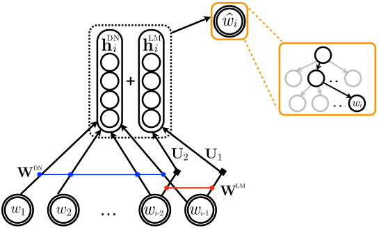
Figure 3: Illustration of the conditional $p(v_{i}|{\bf v}_{<i})$ in a trigram NADE language model. Compared to DocNADE, this model incorporates the architecture of a neural language model, that first maps previous words (2 for a trigram model) to vectors using an embedding matrix ${\bf W}^{\rm LM}$ before connecting them to the hidden layer using regular (untied) parameter matrices (${\bf U_{1}}$, ${\bf U_{2}}$ for a trigram). In our experiments, each conditional $p(v_{i}|{\bf v}_{<i})$ exploits decomposed into a tree of logistic regressions, the hierarchical softmax.

The figure 3 depicts the overall architecture. This model can be seen as an extension of the seminal work on neural language models of Bengio et al. (2003) that includes a representation of a document’s larger context. It can also be seen as a neural extension of the cache-based language model introduced in (Kuhn and Mori, 1990), where the $n$-gram probability is interpolated with the word distribution observed in a dynamic cache. This cache of a fixed size keeps track of previously observed words to include long term dependencies in the prediction and preserve semantic consistency beyond the scope of the $n$-gram. In our case, the DocNADE language model maintains an unbounded cache and define a proper, jointly trained solution to mitigate these two kinds of dependencies.

As in DocNADE, a document ${\bf v}$ is modeled as a sequence of multinomial observations. The sequence size is arbitrary and each element $v_{i}$ consists in the index of the $i$-th word in a vocabulary of size $V$. The conditional probability of a word given its history $p(v_{i}|{\bf v}_{<i})$ is now expressed as a smooth function of a hidden layer ${\bf h}_{i}({\bf v}_{<i})$ used to predict word $v_{i}$. The peculiarity of the DocNADE language model lies in the definition of this hidden layer, which now includes two terms:

$${\bf h}_{i}({\bf v}_{<i})={\bf g}({\bf b}+{\bf h}^{\rm DN}_{i}({\bf v}_{<i})+{\bf h}^{\rm LM}_{i}({\bf v}_{<i})).$$ (14)

The first term borrows from the DocNADE model by aggregating embeddings for all the previous words in the history:

$${\bf h}^{\rm DN}_{i}({\bf v}_{<i})=\sum_{k<i}{\bf W}^{\rm DN}_{:,v_{k}}~{}.$$ (15)

The second contribution derives from neural $n$-gram language models as follows:

$${\bf h}^{\rm LM}_{i}({\bf v}_{<i})=\sum_{k=1}^{n-1}{\bf U}_{k}\cdot{\bf W}^{\rm LM}_{:,v_{i-k}}~{}.$$ (16)

In this formula, the history for the word $v_{i}$ is restricted to the $n-1$ preceding words, following the common $n$-gram assumption. The term ${\bf h}^{\rm LM}_{i}$ hence represents the continuous representation of these $n-1$ words, in which word embeddings are linearly transformed by the ordered matrices ${\bf U}_{1},{\bf U}_{2},...,{\bf U}_{n-1}$. Moreover, ${\bf b}$ gathers the bias terms for the hidden layer. In this model, two sets of word embeddings are defined, ${\bf W}^{\rm DN}$ and ${\bf W}^{\rm LM}$, which are respectively associated to the DocNADE and neural language model parts. For simplicity, we assume both are of the same size $H$.

Given hidden layer ${\bf h}_{i}({\bf v}_{<i})$, conditional probabilities $p(v_{i}|{\bf v}_{<i})$ can be estimated, and thus $p({\bf v})$. For the aforementioned reason, the output layer is structured for efficient computations. Specifically, we decided to use a variation of the probabilistic binary tree, known as a hierarchical softmax layer. In this case, instead of having binary nodes with multiple levels in the tree, we have only two levels where all words have their leaf at level two and each node is a multiclass (i.e. softmax) logistic regression with roughly $\sqrt{V}$ classes (one for each children). Computing probabilities in such a structured layer can be done using only two matrix multiplications, which can be efficiently computed on the GPU.

With a hidden layer of size $H$, the complexity of computing the softmax at one node is $O(H\sqrt{V})$. If we have $D$ words in a given document, the complexity of computing all necessary probabilities from the hidden layers is thus $O(DH\sqrt{V})$. It also requires $O(DH)$ computations to compute the hidden representations for the DocNADE part and $O(nH^{2})$ for the language model part. The full complexity for computing $p({\bf v})$ and the updates for the parameters are thus computed in $O(DH\sqrt{V}+DH+nH^{2})$.

Once again, the loss function of the model is the negative log-likelihood and we minimize it by using stochastic gradient descent over documents, to learn the values of the parameters $\allowbreak\{{\bf b},{\bf c},{\bf V},{\bf W}^{\rm LM},{\bf W}^{\rm DN},{\bf U}_{1},...,{\bf U}_{n}\}$.

5 Related Work

Much like NADE was inspired by the RBM, DocNADE can be seen as related to the Replicated Softmax model (Salakhutdinov and Hinton, 2009), an extension of the RBM to document modeling. Here, we describe in more detail the Replicated Softmax, along with its relationship with DocNADE.

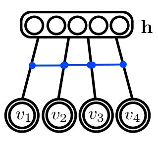
Figure 4: Replicated Softmax model. Each multinomial observation $v_{i}$ is a word. Connections between each multinomial observation $v_{i}$ and hidden units are shared.

Much like the RBM, the Replicated Softmax models observations using a latent, stochastic binary layer ${\bf h}$. Here, the observations are the documents ${\bf v}$, which interact with the hidden layer ${\bf h}$ through an energy function similar to RBM’s:

$$E({\bf v},{\bf h}) =-D~{}{\bf c}^{\top}{\bf h}+\sum_{i=1}^{D}-{\bf h}^{\top}{\bf W}_{:,v_{i}}-b_{v_{i}}=-D~{}{\bf c}^{\top}{\bf h}-{\bf h}^{\top}{\bf W}{\bf n}({\bf v})-{\bf b}^{\top}{\bf n}({\bf v}),$$ (17)

where ${\bf n}({\bf v})$ is a bag-of-word vector of size $V$ (the size of the vocabulary) containing the word count of each word in the vocabulary for document ${\bf v}$. $\bf h$ is the stochastic, binary hidden layer vector and ${\bf W}_{:,v_{i}}$ is the $v_{i}^{\rm th}$ column vector of matrix ${\bf W}$. $\bf c$ and $\bf b$ are the bias vectors for the visible and the hidden layers. We see here that the larger $\bf v$ is, the bigger the number of terms in the sum over $i$ is, resulting in a high energy value. For this reason, the hidden bias term ${\bf c}^{\top}{\bf h}$ is multiplied by $D$, to be commensurate with the contribution of the visible layer.. We can see also that connection parameters are shared across different positions $i$ in ${\bf v}$, as illustrated by figure 4).

The conditional probabilities of the hidden and the visible layer factorize much like in the RBM, in the following way:

$$p({\bf h}|{\bf v})=\prod_{j}p(h_{j}|{\bf v})~{},~{}~{}~{}~{}~{}p({\bf v}|{\bf h})=\prod_{i=1}^{D}p(v_{i}|{\bf h})$$ (18)

where the factors $p(h_{j}|{\bf v})$ and $p(v_{i}|{\bf h})$ are such that

$$p(h_{j}=1|{\bf v}) =\mathrm{sigm}(Dc_{j}+\sum_{i}W_{jv_{i}})$$ (19)

$$p(v_{i}=w|{\bf h}) =\frac{\exp(b_{w}+{\bf h}^{\top}{\bf W}_{:,w})}{\sum_{w^{\prime}}\exp(b_{w^{\prime}}+{\bf h}^{\top}{\bf W}_{:,w^{\prime}})}$$ (20)

The normalized exponential part in $p(v_{i}=w|{\bf h})$ is simply the softmax function. To train this model, we’d like to minimize the negative log-likelihood (NLL). Its gradients for a document ${\bf v}^{(t)}$ with respect to the parameters $\theta=\{{\bf W},{\bf c},{\bf b}\}$ are calculated as follows:

$$\frac{\partial-\log p({\bf v}^{(t)})}{\partial\theta} ={\sf{E\mspace{-8.7mu}E}}_{{\bf h}|{\bf v}^{(t)}}\left[\frac{\partial}{\partial\theta}E({\bf v}^{(t)},{\bf h})\right]-{\sf{E\mspace{-8.7mu}E}}_{{\bf v},{\bf h}}\left[\frac{\partial}{\partial\theta}E({\bf v},{\bf h})\right].$$ (21)

As with conventional RBMs, the second expectation in Equation 21 is computationally too expensive. The gradient of the negative log-likelihood is therefore approximated by replacing the second expectation with an estimated value obtained by contrastive divergence (Hinton, 2002). This approach consists of performing $K$ steps of blocked Gibbs sampling, starting at ${\bf v}^{(t)}$ and using Equations 19 and 20, to obtain point estimates of the expectation over ${\bf v}$. Large values of $K$ must be used to reduce the bias of gradient estimates and obtain good estimates of the distribution. This approximation is used to perform stochastic gradient descent.

During Gibbs sampling, the Replicated Softmax model must compute and sample from $p(v_{i}=w|{\bf h})$, which requires the computation of a large softmax. Most importantly, the computation of the softmax most be repeated $K$ times for each update, which can be prohibitive, especially for large vocabularies. Unlike DocNADE, this softmax cannot simply be replaced by a structured softmax.

It is interesting to see that DocNADE is actually related to how the Replicated Softmax approximates, through mean-field inference, the conditionals $p(v_{i}=w|{\bf v}_{<i})$. Computing the conditional $p(v_{i}=w|{\bf v}_{<i})$ with the Replicated Softmax is intractable. However, we could use mean-field inference to approximate the full conditional $p(v_{i},{\bf v}_{>i},{\bf h}|{\bf v}_{<i})$ as the factorized

$$q(v_{i},{\bf v}_{>i},{\bf h}|{\bf v}_{<i})=\prod_{k\geq i}q(v_{k}|{\bf v}_{<i})\prod_{j}q(h_{j}|{\bf v}_{<i})~{},$$ (22)

where $q(v_{k}=w|{\bf v}_{<i})=\mu_{kw}(i)$ and $q(h_{j}=1|{\bf v}_{<i})=\tau_{j}(i)$. We would find the parameters $\mu_{kw}(i)$ and $\tau_{j}(i)$ that minimize the KL divergence between $q(v_{i},{\bf v}_{>i},{\bf h}|{\bf v}_{<i})$ and $p(v_{i},{\bf v}_{>i},{\bf h}|{\bf v}_{<i})$ by applying the following message passing equations until convergence:

$$\tau_{j}(i)\leftarrow\mathrm{sigm}\left(D~{}c_{j}+\sum_{k\geq i}\sum_{w^{\prime}=1}^{V}W_{jw^{\prime}}\mu_{kw^{\prime}}(i)+\sum_{k<i}W_{jv_{k}}\right),$$ (23)

$$\mu_{kw}(i)\leftarrow\frac{\exp(b_{w}+\sum_{j}W_{jw}\tau_{j}(i))}{\sum_{w^{\prime}}\exp(b_{w^{\prime}}+\sum_{j}W_{jw^{\prime}}\tau_{j}(i))}.$$ (24)

with $k\in\{i,\dots,D\}$, $j\in\{1,\dots,H\}$ and $w\in\{1,\dots,V\}$. The conditional $p(v_{i}=w|{\bf v}_{<i})$ could then be estimated with $\mu_{kw}(i)$ for all $i$. We note that one iteration of mean-field (with $\mu_{kw^{\prime}}(i)$ initialized to 0) in the Replicated Softmax corresponds to the conditional $p(v_{i}=w|{\bf v}_{<i})$ computed by DocNADE with a single hidden layer and a flat softmax output layer.

In our experiment, we’ll see that DocNADE compares favorably to Replicated Softmax.

6 Topic modeling experiments

To compare the topic models, two kinds of quantitative comparisons are used. The first one evaluates the generative ability of the different models, by computing the perplexity of held-out texts. The second one compares the quality of document representations for an information retrieval task.

Two different datasets are used for the experiments of this section, 20 Newsgroups and RCV1-V2 (Reuters Corpus Volume I). The 20 Newsgroups corpus has 18,786 documents (postings) partitioned into 20 different classes (newsgroups). RCV1-V2 is a much bigger dataset composed of 804,414 documents (newswire stories) manually categorized into 103 classes (topics). The two datasets were preprocessed by stemming the text and removing common stop-words. The 2,000 most frequent words of the 20 Newsgroups training set and the 10,000 most frequent words of the RCV1-V2 training set were used to create the dictionary for each dataset. Also, every word counts $n_{i}$, used to represent the number of times a word appears in a document was replaced by $log(1+n_{i})$ rounded to the nearest integer, following Salakhutdinov and Hinton (2009).

6.1 Generative Model Evaluation

For the generative model evaluation, we follow the experimental setup proposed by Salakhutdinov and Hinton (2009) for 20 Newsgroups and RCV1-V2 datasets. We use the exact same split for the sake of comparison. The setup consists in respectively 11,284 and 402,207 training examples for 20 Newsgroups and RCV1-V2. We randomly extracted 1,000 and 10,000 documents from the training sets of 20 Newsgroups and RCV1-V2, respectively, to build a validation set. The average perplexity per word is used for comparison. This perplexity is estimated using the 50 first test documents, as follows:

$$\exp\left(-\frac{1}{T}\sum_{t}\frac{1}{|{\bf v}^{t}|}\log p({\bf v}^{t})\right),$$ (25)

where $T$ is the total number of examples and ${\bf v}^{t}$ is the $t^{\rm th}$ test document.

Dataset	LDA	Replicated	fDARN	DocNADE	DeepDN	DeepDN	DeepDN
		Softmax			(1layer)	(2layer)	(3layer)
20 News	1091	953	917	896	835	877	923
RCV1-v2	1437	988	724	742	579	552	539

Table 1: Test perplexity per word for models with 50 topics. The results for LDA and Replicated Softmax were taken from Salakhutdinov and Hinton (2009).

Table 1 gathers the perplexity per word results for 20 Newsgroups and RCV1-V2. Theere we compare 5 different models: the Latent Dirichlet Allocation (LDA) (Blei et al., 2003), the Replicated Softmax, the recent fast Deep AutoRegressive Networks (fDARN) (Mnih and Gregor, 2014), DocNADE and DeepDocNADE (DeepDN in the table). Each model uses 50 latent topics. For the experiments with DeepDocNADE, we provide the performance when using 1, 2, and 3 hidden layers. As shown in Table 1, DeepDocNADE provides the best generative performances. Our best DeepDocNADE models were trained with the Adam optimizer (Kingma and Ba, 2014) and with the tanh activation function. The hyper-parameters of Adam were selected on the validation set.

Crucially, following Uria et al. (2014), an ensemble approach is used to compute the probability of documents, where each component of the ensembles are the same DeepDocNADE model evaluated on a different word ordering. Specifically, the perplexity with $M$ ensembles becomes as follows:

$$\exp\left(-\frac{1}{T}\sum_{t}\frac{1}{|{\bf v}^{t}|}\log\left(\frac{1}{M}\sum_{m}p({\bf v}^{(t,m)})\right)\right),$$ (26)

where $T$ is the total number of examples, $M$ is the number of ensembles (word orderings) and ${\bf v}^{(t,m)}$ denotes the $m^{\rm th}$ word ordering for the $t^{\rm th}$ documnet. We try $M=\left\{1,2,4,16,32,64,128,256\right\}$, with the results in Table 1 using $M=256$. For the 20 Newsgroups dataset, adding more hidden layers to DocDocNADE fails to provide further improvements. We hypothesize that the relatively small size of this dataset makes it hard to successfully train a deep model. However, the opposite is observed on the RCV1-V2 dataset, which is more than an order of magnitude larger than 20 Newsgroups. In this case, DeepDocNADE outperforms fDARN and DocNADE, with a relative perplexity reduction of 20%, 24% and 26% with respectively 1,2 and 3 hidden layers.

To illustrate the impact of $M$ on the performance of DeepDocNADE, Figure 5 shows the perplexity on both datasets using the different values for $M$ that we tried. We can observe that beyond $M=128$, this hyper-parameter has only a minimal impact on the perplexity.

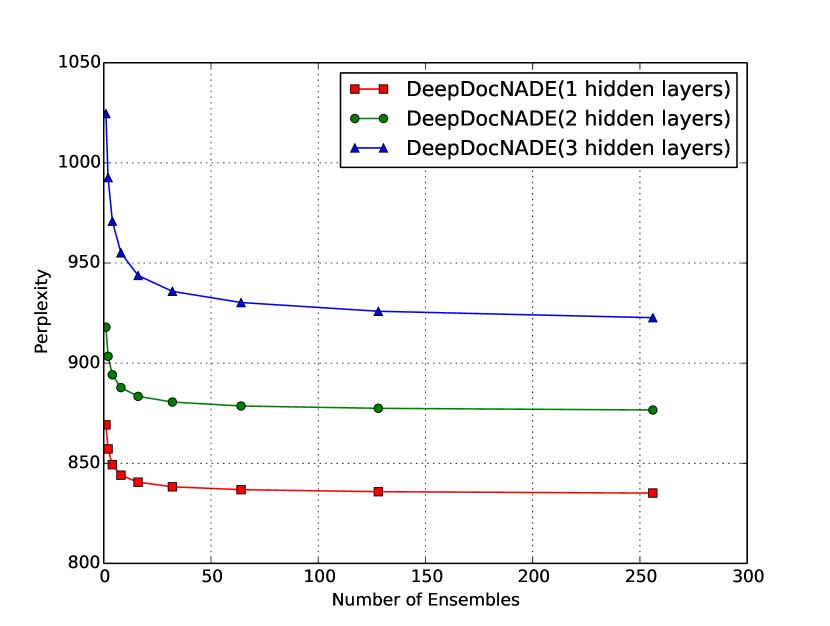
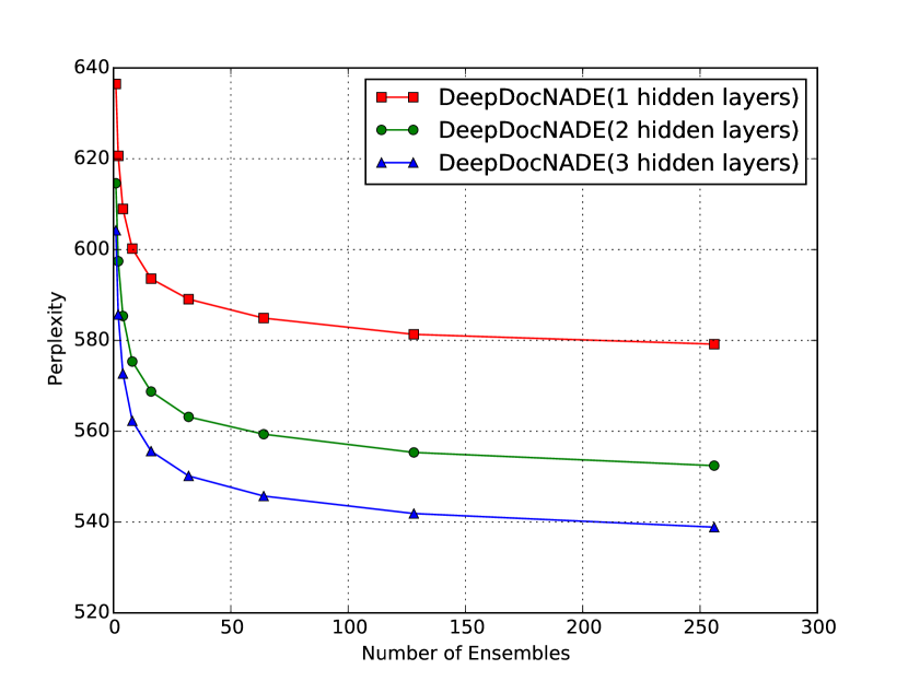
Figure 5: Perplexity obtained with different numbers of word orderings $m$ for 20 Newsgroups on the left and RCV1-V2 on the right.

6.2 Document Retrieval Evaluation

A document retrieval evaluation task was also used to evaluate the quality of the document representation learned by each model. As in the previous section, the datasets under consideration are 20 Newsgroups and RCV1-V2. The experimental setup is the same for the 20 Newsgroups dataset, while for the RCV1-V2 dataset, we reproduce the same setup as the one used in Srivastava et al. (2013), where the training set contained 794,414 examples and 10,000 examples constituted the test set.

For DocNADE and DeepDocNADE, the representation of a document is obtained simply by computing the top-most hidden layer when feeding all words as input.

The retrieval task follows the setup of Srivastava et al. (2013). The documents in the training and validation sets are used as the database for retrieval, while the test set is used as the query set. The similarity between a query and all examples in the database is computed using the cosine similarity between their vector representations. For each query, documents in the database are then ranked according to this similarity, and precision/recall (PR) curves are computed, by comparing the label of the query documents with those of the database documents. Since documents sometimes have multiple labels (specifically those in RCV1-V2), for each query the PR curves for each of its labels are computed individually and then averaged. Finally, we report the global average of these (query-averaged) curves to compare models against each other. Training and model selection is otherwise performed as in the generative modeling evaluation.

As shown in Figure 6, DeepDocNADE always yields very competitive results, on both datasets, and outperforming the other models in most cases. Specifically, for the 20 Newsgroups dataset, DeepDocNADE with 2 and 3 hidden layers always perform better than the other methods. DeepDocNADE with 1 hidden layer also performs better than the other baselines when retrieving the top few documents ( e.g. when recall is smaller than 0.2).

20 NewsGroups

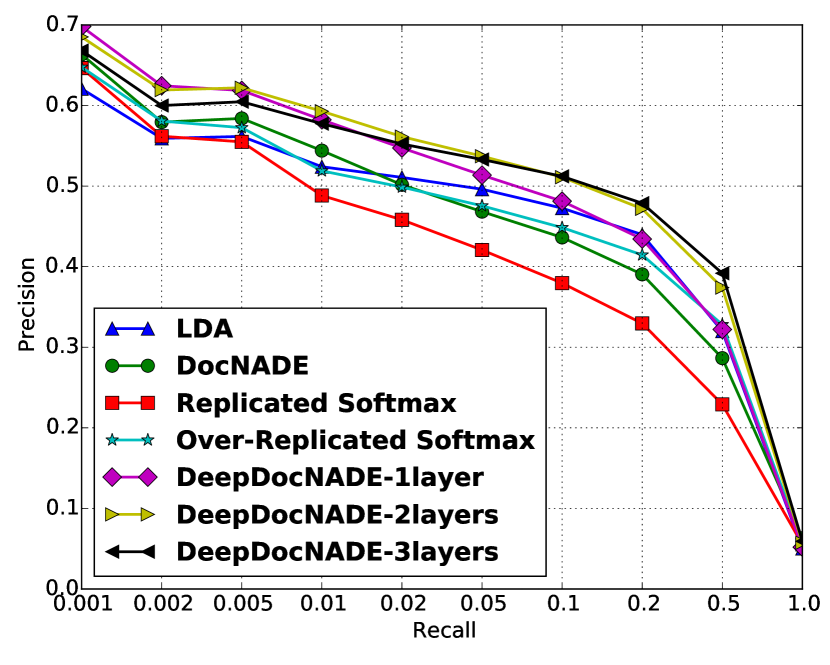
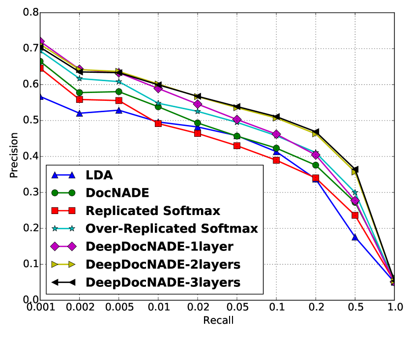
Reuters RCV1-V2

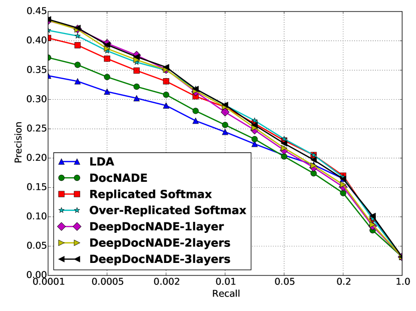
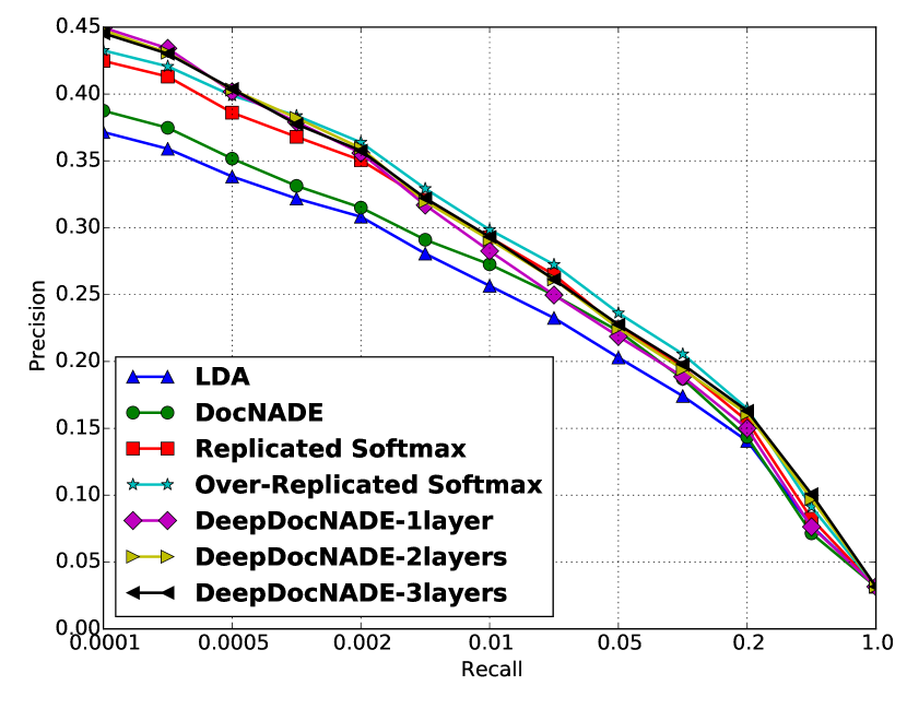
Figure 6: Precision-Recall curves for document retrieval task. On the left are the results using a hidden layer size of 128, while the plots on the right are for a size of 512.

6.3 Qualitative Inspection of Learned Representations

In this section, we want to assess if the DocNADE approach for topic modeling can capture meaningful semantic properties of texts.

First, one way to explore the semantic properties of trained models is through their learned word embeddings. Each of the columns of the matrix $W$ represents a word $w$ where $W_{:,w}$ is the vector representation of $w$. Table 3 shows for some chosen words the five nearest words according to their embeddings, foro a DocNADE model. We can observe for each example the semantic consistency of the word representations. Similar results can be observed for DeepDocNADE models.

weapons	medical	companies	define	israel	book	windows
weapon	treatment	demand	defined	israeli	reading	dos
shooting	medecine	commercial	definition	israelis	read	microsoft
firearms	patients	agency	refer	arab	books	version
assault	process	company	make	palestinian	relevent	ms
armed	studies	credit	examples	arabs	collection	pc

Table 2: The five nearest neighbors in the word representation space learned by DocNADE.

We’ve also attempted to measure whether the hidden units of the first hidden layer of DocNADE and DeepDocNADE models modeled distinct topics. Understanding the function represented by hidden units in neural networks is not a trivial affair, but we considered the following, simple approach. For a given hidden unit, its connections to words were interpreted as the importance of the word for the associated topic. Therefore, for a hidden unit, we selected the words having the strongest positive connections, i.e.  for the $i_{th}$ hidden unit we chose the words $w$ that have the highest connection values $W_{i,w}$.

With this approach, four topics were obtained from a DocNADE model using the sigmoid activation function and trained on 20 Newsgroups, as shown in Table 3 and can be readily interpreted as topics representing religion, space, sports and security. Note that those four topics are actually (sub)categories in 20 Newsgroups.

That said, we’ve had less success understanding the topics extracted when using the tanh activation function or when using DeepDocNADE. It thus seems that these models are then choosing to learn a latent representation that isn’t aligning its dimensions with concepts that are easily interpretable, even though it is clearly capturing well the statistics of documents (since our qualitative results with DeepDocNADE are excellent).

Hidden unit topics
jesus	shuttle	season	encryption
atheism	orbit	players	escrow
christianity	lunar	nhl	pgp
christ	spacecraft	league	crypto
athos	nasa	braves	nsa
atheists	space	playoffs	rutgers
bible	launch	rangers	clipper
christians	saturn	hockey	secure
sin	billion	pitching	encrypted
atheist	satellite	team	keys

Table 3: Illustration of some topics learned by DocNADE. A topic $i$ is visualized by picking the 10 words $w$ with strongest connection $W_{iw}$.

7 Language Modeling Experiments

In this section, we test whether our proposed approach to incorporating a DocNADE component to a neural language model can improve the performance of a neural language model. Specifically, we considered treating a text corpus as a sequence of documents. We used the APNews dataset, as provided by Mnih and Hinton (2009). Unfortunately, information about the original segmentation into documents of the corpus wasn’t available in the data as provided by Mnih and Hinton (2009), thus we simulated the presence of documents by grouping one or more adjacent sentences, for training and evaluating DocNADE-LM, making sure the generated documents were non-overlapping. Thankfully, this approach still allows us to test whether DocNADE-LM is able to effectively leverage the larger context of words in making its predictions.

Since language models are generative models, the perplexity measured on some held-out texts provides an intrinsic and widely used evaluation criterion. Following Mnih and Hinton (2007) and Mnih and Hinton (2009), we used the APNews dataset containing Associated Press news stories from 1995 and 1996. The dataset is again split into training, validation and test sets, with respectively 633,143, 43,702 and 44,601 sentences. The vocabulary is composed of 17,964 words. A 100 dimensional feature vectors are used for these experiments. The validation set is used for model selection and the perplexity scores of Table 4 are computed on the test set.

Models	Number of grouped sentences	Perplexity
KN5	-	123.2
KN6	-	123.5
LBL	-	117.0
HLBL	-	112.1
FFN	-	119.78
DocNADE-LM	1	111.93
DocNADE-LM	2	110.9
DocNADE-LM	3	109.8
DocNADE-LM	4	109.78
DocNADE-LM	5	109.22

Table 4: Test perplexity per word for models with 100 topics. The results for HLBL and LBL were taken from Mnih and Hinton (2009).

The FFN model in Table 4 corresponds to a regular neural (feed-forward) network language model. It is equivalent to setting ${\bf h}^{\rm DN}_{i}({\bf v}_{<i})$ to zero in Equation 14. These results are meant to measure whether the DocNADE part of DocNADE-LM can indeed help to improve performances.

We also compare to the log-bilinear language (LBL) model of Mnih and Hinton (2007)). While for the FFN model we used a hierarchical softmax to compute the conditional word probabilities (see Section 4), the LBL model uses a full softmax output layer that uses the same word representation matrix at the input and output. This latter model is therefore slower to train. Later, Mnih and Hinton (2009) also proposed adaptive approaches to learning a structured softmax layer, thus we also compare with their best approach. All aforementioned baselines are 6-gram models, taking in consideration the last 5 previous words to predict the next one. We also compare with more traditional 5-gram and 6-gram models using Kneser-Ney smoothing, taken from Mnih and Hinton (2007).

From Table 4, we see that adding context to DocNADE-LM, by increasing the size of the multi-sentence segments, significantly improves the performance of the model (compared to FFN) and also surpasses the performance of the most competitive alternative, the HLBL model.

7.1 Qualitative Inspection of Learned Representations

In this section we explore the semantic properties of texts learned by the DocNADE-LM model. Interestingly, we can examine the two different components (DN and LM) separately. Because the DocNADE part and the language modeling part of the model each have their own word matrix, ${\bf W}^{\rm DN}$ and ${\bf W}^{\rm LM}$ respectively, we can compare their contribution through these learned embeddings. As explained in the previous section, each of the columns of the matrices represents a word $w$ where ${\bf W}^{\rm DN}_{:,w}$ and ${\bf W}^{\rm LM}_{:,w}$ are two different vector representations of the same word $w$.

We can see by observing Tables 5 and 6 that the two parts of the DocNADE-LM model have learned different semantic properties of words. An interesting example is seen in the nearest neighbors of the word israel, where the DocNADE focuses on the politico-cultural relation between these words, whereas the language model part seems to have learned the concept of countries in general.

weapons	medical	companies	define	israel	book	windows
security	doctor	industry	spoken	israeli	story	yards
humanitarian	health	corp	to	palestinian	novel	rubber
terrorists	medicine	firms	think_of	jerusalem	author	piled
deployment	physicians	products	of	lebanon	joke	fire_department
diplomats	treatment	company	bottom_line	palestinians	writers	shell

Table 5: The five nearest neighbors in the word representation space learned by the DocNADE part of the DocNADE-LM model.

weapons	medical	companies	define	israel	book	windows
systems	special	countries	talk_about	china	film	houses
aircraft	japanese	nations	place	russia	service	room
drugs	bank	states	destroy	cuba	program	vehicle
equipment	media	americans	show	north_korea	movie	restaurant
services	political	parties	over	lebanon	information	car

Table 6: The five nearest neighbors in the word representation space learned by the language model part of the DocNADE-LM model.

8 Conclusion

We have presented models inspired by NADE that can achieve state-of-the-art performances for modeling documents.

Indeed, for topic modeling, DocNADE had competitive results while its deep version, DeepDocNADE, outperformed the current state-of-the-art in generative document modeling, based on test set perplexity. The similarly good performances where observed when we used these models as feature extractors to represent documents for the task of information retrieval.

As for language modeling, the competitive performances of the DocNADE language models showed that combining contextual information by leveraging the DocNADE neural network architecture can significantly improve the performance of a neural probabilistic N-gram language model.

References

- Bengio et al. (2003) Yoshua Bengio, Réjean Ducharme, Pascal Vincent, and Christian Janvin. A neural probabilistic language model. The Journal of Machine Learning Research, 3:1137–1155, 2003.
- Blei et al. (2003) David M. Blei, Andrew Y. Ng, and Michael I. Jordan. Latent Dirichlet Allocation. Journal of Machine Learning Research, 3(4-5):993–1022, 2003.
- Chang et al. (2009) Jonathan Chang, Jordan Boyd-Graber, Sean Gerrish, Chong Wang, and David Blei. Reading Tea Leaves: How Humans Interpret Topic Models. In Advances in Neural Information Processing Systems 22 (NIPS 2009), pages 288–296, 2009.
- Hinton (2002) Geoffrey E. Hinton. Training products of experts by minimizing contrastive divergence. Neural Computation, 14:1771–1800, 2002.
- Kingma and Ba (2014) Diederik Kingma and Jimmy Ba. Adam: A method for stochastic optimization. arXiv preprint arXiv:1412.6980, 2014.
- Kuhn and Mori (1990) R. Kuhn and R. De Mori. A cache-based natural language model for speech recognition. IEEE Transactions on Pattern Analysis and Machine Intelligence, 12(6):570–583, june 1990.
- Larochelle and Lauly (2012) Hugo Larochelle and Stanislas Lauly. A neural autoregressive topic model. In Advances in Neural Information Processing Systems, pages 2708–2716, 2012.
- Larochelle and Murray (2011) Hugo Larochelle and Ian Murray. The Neural Autoregressive Distribution Estimator. In Proceedings of the 14th International Conference on Artificial Intelligence and Statistics (AISTATS 2011), volume 15, pages 29–37, Ft. Lauderdale, USA, 2011. JMLR W&CP.
- Mnih and Gregor (2014) Andriy Mnih and Karol Gregor. Neural variational inference and learning in belief networks. arXiv preprint arXiv:1402.0030, 2014.
- Mnih and Hinton (2007) Andriy Mnih and Geoffrey Hinton. Three new graphical models for statistical language modelling. In Proceedings of the 24th international conference on Machine learning, pages 641–648. ACM, 2007.
- Mnih and Hinton (2009) Andriy Mnih and Geoffrey E Hinton. A Scalable Hierarchical Distributed Language Model. In Advances in Neural Information Processing Systems 21 (NIPS 2008), pages 1081–1088, 2009.
- Morin and Bengio (2005) Frederic Morin and Yoshua Bengio. Hierarchical Probabilistic Neural Network Language Model. In Proceedings of the 10th International Workshop on Artificial Intelligence and Statistics (AISTATS 2005), pages 246–252. Society for Artificial Intelligence and Statistics, 2005.
- Salakhutdinov and Hinton (2009) Ruslan Salakhutdinov and Geoffrey Hinton. Replicated Softmax: an Undirected Topic Model. In Advances in Neural Information Processing Systems 22 (NIPS 2009), pages 1607–1614, 2009.
- Srivastava et al. (2013) Nitish Srivastava, Ruslan R Salakhutdinov, and Geoffrey E Hinton. Modeling documents with deep boltzmann machines. arXiv preprint arXiv:1309.6865, 2013.
- Tomas Mikolov (2013) Greg Corrado Jeffrey Dean Tomas Mikolov, Kai Chen. Efficient Estimation of Word Representations in Vector Space. In Workshop Track of the 1st International Conference on Learning Representations (ICLR 2013), 2013.
- Uria et al. (2014) Benigno Uria, Iain Murray, and Hugo Larochelle. A deep and tractable density estimator. JMLR: W&CP, 32(1):467–475, 2014.
- Zheng et al. (2015) Yin Zheng, Yu-Jin Zhang, and Hugo Larochelle. A deep and autoregressive approach for topic modeling of multimodal data. TPAMI, 2015.