Parameterized vertex deletion problems for hereditary graph classes with a block property

Abstract

For a class of graphs $\mathcal{P}$, the Bounded $\mathcal{P}$-Block Vertex Deletion problem asks, given a graph $G$ on $n$ vertices and positive integers $k$ and $d$, whether there is a set $S$ of at most $k$ vertices such that each block of $G-S$ has at most $d$ vertices and is in $\mathcal{P}$. We show that when $\mathcal{P}$ satisfies a natural hereditary property and is recognizable in polynomial time, Bounded $\mathcal{P}$-Block Vertex Deletion can be solved in time $2^{\mathcal{O}(k\log d)}n^{\mathcal{O}(1)}$. When $\mathcal{P}$ contains all split graphs, we show that this running time is essentially optimal unless the Exponential Time Hypothesis fails. On the other hand, if $\mathcal{P}$ consists of only complete graphs, or only cycle graphs and $K_{2}$, then Bounded $\mathcal{P}$-Block Vertex Deletion admits a $c^{k}n^{\mathcal{O}(1)}$-time algorithm for some constant $c$ independent of $d$. We also show that Bounded $\mathcal{P}$-Block Vertex Deletion admits a kernel with $\mathcal{O}(k^{2}d^{7})$ vertices.

1 Introduction

Vertex deletion problems are formulated as follows: given a graph $G$ and a class of graphs $\mathcal{G}$, is there a set of at most $k$ vertices whose deletion transforms $G$ into a graph in $\mathcal{G}$? A graph class $\mathcal{G}$ is hereditary if whenever $G$ is in $\mathcal{G}$, every induced subgraph $H$ of $G$ is also in $\mathcal{G}$. Lewis and Yannakakis [16] proved that for every non-trivial hereditary graph class decidable in polynomial time, the vertex deletion problem for this class is NP-complete. On the other hand, a class is hereditary if and only if it can be characterized by a set of forbidden induced subgraphs $\mathcal{F}$, and Cai [3] showed that if $\mathcal{F}$ is finite, with each graph in $\mathcal{F}$ having at most $c$ vertices, then there is an $\mathcal{O}(c^{k}n^{c+1})$-time algorithm for the corresponding vertex deletion problem.

A block of a graph is a maximal connected subgraph not containing a cut vertex. Every maximal $2$-connected subgraph is a block, but a block may just consist of one or two vertices. We consider vertex deletion problems for hereditary graph classes where all blocks of a graph in the class satisfy a certain common property. It is natural to describe such a class by the set of permissible blocks $\mathcal{P}$. For ease of notation, we do not require that $\mathcal{P}$ is itself hereditary, but the resulting class, where graphs consist of blocks in $\mathcal{P}$, should be. To achieve this, we say that a class of graphs $\mathcal{P}$ is block-hereditary if, whenever $G$ is in $\mathcal{P}$ and $H$ is an induced subgraph of $G$, every block of $H$ with at least one edge is isomorphic to a graph in $\mathcal{P}$. For a block-hereditary class of graphs $\mathcal{P}$, we define $\Phi_{\mathcal{P}}$ as the class of all graphs whose blocks with at least one edge are in $\mathcal{P}$. Several well-known graph classes can be defined in this way. For instance, a forest is a graph in the class $\Phi_{\{K_{2}\}}$, a cactus graph is a graph in the class $\Phi_{\mathcal{C}}$ where $\mathcal{C}$ consists of $K_{2}$ and all cycles, and a complete-block graph is a graph in $\Phi_{\mathcal{K}}$ where $\mathcal{K}$ consists of all complete graphs. We note that $\mathcal{C}$ is not a hereditary class, but it is block-hereditary; this is what motivates our use of the term.

Let $\mathcal{P}$ be a block-hereditary class such that $\Phi_{\mathcal{P}}$ is a non-trivial hereditary class. The result of Lewis and Yannakakis [16] implies that the vertex deletion problem for $\Phi_{\mathcal{P}}$ is NP-complete. We define the following parameterized problem for a fixed block-hereditary class of graphs $\mathcal{P}$.  
$\mathcal{P}$-Block Vertex Deletion Parameter: $k$ Input: A graph $G$ and a non-negative integer $k$. Question: Is there a set $S\subseteq V(G)$ with $\lvert S\rvert\leqslant k$ such that each block of $G-S$ with at least one edge is in $\mathcal{P}$?

This problem generalizes the well-studied parameterized problems Vertex Cover, when $\mathcal{P}=\emptyset$, and Feedback Vertex Set, when $\mathcal{P}=\{K_{2}\}$. Moreover, if $\Phi_{\mathcal{P}}$ can be characterized by a finite set of forbidden induced subgraphs, then Cai’s approach [3] can be used to obtain a fixed-parameter tractable (FPT) algorithm that runs in time $2^{\mathcal{O}(k)}n^{\mathcal{O}(1)}$.

In this paper, we are primarily interested in the variant of this problem where, additionally, the number of vertices in each block is at most $d$. The value $d$ is a parameter given in the input.  
Bounded $\mathcal{P}$-Block Vertex Deletion Parameter: $d$, $k$ Input: A graph $G$, a positive integer $d$, and a non-negative integer $k$. Question: Is there a set $S\subseteq V(G)$ with $\lvert S\rvert\leqslant k$ such that each block of $G-S$ with at least one edge has at most $d$ vertices and is in $\mathcal{P}$?

We also consider this problem when parameterized only by $k$. When $d=|V(G)|$, this problem is equivalent to $\mathcal{P}$-Block Vertex Deletion, so Bounded $\mathcal{P}$-Block Vertex Deletion is NP-complete for any $\mathcal{P}$ such that $\Phi_{\mathcal{P}}$ is a non-trivial hereditary class. When $d=1$, this problem is equivalent to Vertex Cover. This implies that the Bounded $\mathcal{P}$-Block Vertex Deletion problem is para-NP-hard when parameterized only by $d$.

The Bounded $\mathcal{P}$-Block Vertex Deletion problem is also equivalent to Vertex Cover when $\mathcal{P}$ is a class of edgeless graphs. Since Vertex Cover is well studied, we assume that $d\geqslant 2$, and focus on classes that contain a graph with at least one edge. We call such a class non-degenerate. When $\mathcal{P}$ is the class of all connected graphs with no cut vertices, we refer to Bounded $\mathcal{P}$-Block Vertex Deletion as Bounded Block VD.

Related Work.

The analogue of Bounded Block VD for connected components, rather than blocks, is known as Component Order Connectivity. For this problem, the question is whether a given graph $G$ has a set of vertices $S$ of size at most $k$ such that each connected component of $G-S$ has at most $d$ vertices. Drange et al. [6] showed that Component Order Connectivity is $W[1]$-hard when parameterized by $k$ or by $d$, but FPT when parameterized by $k+d$, with an algorithm running in $2^{\mathcal{O}(k\log d)}n$ time.

Clearly, the vertex deletion problem for either cactus graphs, or complete-block graphs, is a specialization of $\mathcal{P}$-Block Vertex Deletion. A graph is a cactus graph if and only if it does not contain a subdivision of the diamond [7], the graph obtained by removing an edge from the complete graph on four vertices. For this reason, the problem for cactus graphs is known as Diamond Hitting Set. For block graphs, we call it Complete Block Vertex Deletion. General results imply that there is a $c^{k}n^{\mathcal{O}(1)}$-time algorithm for Diamond Hitting Set [9, 12, 14], but an exact value for $c$ is not forthcoming from these approaches. However, Kolay et al. [15] obtained a $12^{k}n^{\mathcal{O}(1)}$-time randomized algorithm. For the variant where each cycle must additionally be odd (that is, $\mathcal{P}$ consists of $K_{2}$ and all odd cycles), there is a $50^{k}n^{\mathcal{O}(1)}$-time deterministic algorithm due to Misra et al. [18]. For Complete Block Vertex Deletion, Kim and Kwon [13] showed that there is an algorithm that runs in $10^{k}n^{\mathcal{O}(1)}$ time, and there is a kernel with $\mathcal{O}(k^{6})$ vertices. Agrawal et al. [1] improved this running time to $4^{k}n^{\mathcal{O}(1)}$, and also obtained a kernel with $\mathcal{O}(k^{4})$ vertices.

When considering a minor-closed class, rather than a hereditary class, the vertex deletion problem is known as $\mathcal{F}$-minor-free Deletion. Every $\mathcal{F}$-minor-free Deletion problem has an $\mathcal{O}(f(k)\cdot n^{3})$-time FPT algorithm [20]. When $\mathcal{F}$ is a set of connected graphs containing at least one planar graph, Fomin et al. [9] showed there is a deterministic FPT algorithm for this problem running in time $2^{\mathcal{O}(k)}\cdot\mathcal{O}(n\log^{2}n)$. One can observe that the class of all graphs whose blocks have size at most $d$ is closed under taking minors. Thus, $\mathcal{P}$-Block Vertex Deletion has a single-exponential FPT algorithm and a polynomial kernel, when $\mathcal{P}$ contains all connected graphs with no cut vertices and at most $d$ vertices. However, it does not tell us anything about the parameterized complexity of Bounded $\mathcal{P}$-Block Vertex Deletion, which we consider in this paper.

Our Contribution.

The main contribution of this paper is the following:

Theorem 1.1

Let $\mathcal{P}$ be a non-degenerate block-hereditary class of graphs that is recognizable in polynomial time. Then, Bounded $\mathcal{P}$-Block Vertex Deletion

1. can be solved in $2^{\mathcal{O}(k\log d)}n^{\mathcal{O}(1)}$ time, and

2. admits a kernel with $\mathcal{O}(k^{2}d^{7})$ vertices.

We will show that this running time is essentially optimal when $\Phi_{\mathcal{P}}$ is the class of all graphs, unless the Exponential Time Hypothesis (ETH) [11] fails. One may expect that if the permissible blocks in $\mathcal{P}$ have a simpler structure, then the problem becomes easier. However, we obtain the same lower bound when $\Phi_{\mathcal{P}}$ contains all split graphs. Since split graphs are a subclass of chordal graphs, the same can be said when $\Phi_{\mathcal{P}}$ contains all chordal graphs.

Theorem 1.2 ()

Let $\mathcal{P}$ be a block-hereditary class. If $\Phi_{\mathcal{P}}$ contains all split graphs, then Bounded $\mathcal{P}$-Block Vertex Deletion is not solvable in time $2^{o(k\log d)}$, unless the ETH fails.

Formally, there is no function $f(x)=o(x)$ such that there is a $2^{f(k\log d)}n^{\mathcal{O}(1)}$-time algorithm for Bounded $\mathcal{P}$-Block Vertex Deletion, unless the ETH fails.

Proposition 1 ()

Let $\mathcal{P}$ be a block-hereditary class. If $\Phi_{\mathcal{P}}$ contains all split graphs, then Bounded $\mathcal{P}$-Block Vertex Deletion is $W[1]$-hard when parameterized only by $k$.

On the other hand, Bounded $\mathcal{P}$-Block Vertex Deletion is FPT when parameterized only by $k$ if $\mathcal{P}$ consists of all complete graphs, or if $\mathcal{P}$ consists of $K_{2}$ and all cycles. We refer to these problems as Bounded Complete Block VD and Bounded Cactus Graph VD respectively.

Theorem 1.3 ()

Bounded Complete Block VD can be solved in time $\mathcal{O}^{*}(10^{k})$.

Theorem 1.4 ()

Bounded Cactus Graph VD can be solved in time $\mathcal{O}^{*}(26^{k})$.

When $d=|V(G)|$, these become $\mathcal{O}^{*}(c^{k})$-time algorithms for Complete Block Vertex Deletion and Diamond Hitting Set respectively. In particular, the latter implies that there is a deterministic FPT algorithm that solves Diamond Hitting Set, running in time $\mathcal{O}^{*}(26^{k})$.

The paper is structured as follows. In the next section, we give some preliminary definitions. In Section 3, we define $\mathcal{P}$-clusters and $\mathcal{P}$-clusterable graphs, and show that $\mathcal{P}$-Block Vertex Deletion can be solved in $\mathcal{O}^{*}(4^{k})$ time for $\mathcal{P}$-clusterable graphs; in particular, we use this to prove Theorem 1.1(i). In Section 4.1, we show that, assuming the ETH holds, this running time is essentially tight (Theorem 1.2), and in Section 4.2 we prove Proposition 1. In Section 5, we use iterative compression to prove Theorems 1.3 and 1.4. Finally, in Section 6, we show that Bounded $\mathcal{P}$-Block Vertex Deletion admits a polynomial kernel, proving Theorem 1.1(ii). We also show that smaller kernels can be obtained for Bounded Block VD, Bounded Complete Block VD, and Bounded Cactus Graph VD.

2 Preliminaries

All graphs considered in this paper are undirected, and have no loops and no parallel edges. Let $G$ be a graph. We denote by $N_{G}(v)$ the set of neighbors of a vertex $v$ in $G$, and let $N_{G}(S):=\bigcup_{v\in S}N_{G}(v)\setminus S$ for any set of vertices $S$. For $X\subseteq V(G)$, the deletion of $X$ from $G$ is the graph obtained by removing $X$ and all edges incident to a vertex in $X$, and is denoted $G-X$. For $x\in V(G)$, we simply use $G-x$ to refer to $G-\{x\}$. Let $\mathcal{F}$ be a set of graphs; then $G$ is $\mathcal{F}$-free if it has no induced subgraph isomorphic to a graph in $\mathcal{F}$. For $n\geqslant 1$, the complete graph on $n$ vertices is denoted $K_{n}$.

A vertex $v$ of $G$ is a cut vertex if the deletion of $v$ from $G$ increases the number of connected components. We say $G$ is biconnected if it is connected and has no cut vertices. A block of $G$ is a maximal biconnected subgraph of $G$. The graph $G$ is $2$-connected if it is biconnected and $\lvert V(G)\rvert\geqslant 3$. In this paper we are frequently dealing with blocks, so the notion of being biconnected is often more natural than that of being $2$-connected. The block tree of $G$ is a bipartite graph $B(G)$ with bipartition $(\mathcal{B},X)$, where $\mathcal{B}$ is the set of blocks of $G$, $X$ is the set of cut vertices of $G$, and a block $B\in\mathcal{B}$ and a cut vertex $x\in X$ are adjacent in $B(G)$ if and only if $B$ contains $x$. A block $B$ of $G$ is a leaf block if $B$ is a leaf of the block tree $B(G)$. Note that a leaf block has at most one cut vertex.

For $u,v\in V(G)$, a $uv$-path is a path beginning at $u$ and ending at $v$. For $X\subseteq V(G)$, an $X$-path is a path beginning and ending at distinct vertices in $X$, with no internal vertices in $X$. For $v\in V(G)$ and $X\subseteq V(G)$, a $(v,X)$-path is a path beginning at $v$, ending at a vertex $x\in X$, and with no internal vertices in $X$. The length of a path $P$, denoted $l(P)$, is the number of edges in $P$. A path is non-trivial if it has length at least two.

Parameterized Complexity. A parameterized problem $Q\subseteq\Sigma^{*}\times N$ is fixed-parameter tractable (FPT) if there is an algorithm that decides whether $(x,k)$ belongs to $Q$ in time $f(k)\cdot\lvert x\rvert^{\mathcal{O}(1)}$ for some computable function $f$. Such an algorithm is called an FPT algorithm. A parameterized problem is said to admit a polynomial kernel if there is a polynomial time algorithm in $\lvert x\rvert+k$, called a kernelization algorithm, that reduces an input instance into an instance with size bounded by a polynomial function in $k$, while preserving the Yes or No answer.

3 Clustering

Agrawal et al. [1] described an efficient FPT algorithm for Complete Block Vertex Deletion using a two stage approach. Firstly, small forbidden induced subgraphs are eliminated using a branching algorithm. More specifically, for each diamond or cycle of length four, at least one vertex must be removed in a solution, so there is a branching algorithm that runs in $\mathcal{O}^{*}(4^{k})$ time. The resulting graph has the following structural property: any two distinct maximal cliques have at most one vertex in common. Thus, in the second stage, it remains only to eliminate all cycles not fully contained in a maximal clique, so the problem can be reduced to an instance of Weighted Feedback Vertex Set. We generalize this process and refer to it as “clustering”, where the “clusters”, in the case of Complete Block Vertex Deletion, are the maximal cliques. We use this to obtain an algorithm for Bounded $\mathcal{P}$-Block Vertex Deletion in Section 3.2.

3.1 $\mathcal{P}$-clusters

Let $\mathcal{P}$ be a block-hereditary class of graphs. We may assume that $\mathcal{P}$ contains only biconnected graphs; otherwise there is some block-hereditary $\mathcal{P}^{\prime}$ such that $\mathcal{P}^{\prime}\subset\mathcal{P}$ and $\Phi_{\mathcal{P}^{\prime}}=\Phi_{\mathcal{P}}$. Let $G$ be a graph. A $\mathcal{P}$-cluster of $G$ is a maximal induced subgraph $H$ of $G$ with the property that $H$ is isomorphic either to $K_{1}$ or a graph in $\mathcal{P}$. We say that $G$ is $\mathcal{P}$-clusterable if for any distinct $\mathcal{P}$-clusters $H_{1}$ and $H_{2}$ of $G$, we have $|V(H_{1})\cap V(H_{2})|\leqslant 1$. For a $\mathcal{P}$-clusterable graph, if $v\in V(G)$ is contained in at least two distinct $\mathcal{P}$-clusters, then $v$ is called an external vertex.

The following property of $\mathcal{P}$-clusters is essential. We say that $X\subseteq V(G)$ hits a cycle $C$ if $X\cap V(C)\neq\emptyset$, and a cycle $C$ is contained in a $\mathcal{P}$-cluster of $G$ if $V(C)\subseteq V(H)$ for some $\mathcal{P}$-cluster $H$ of $G$.

Lemma 1

Let $\mathcal{P}$ be a non-degenerate block-hereditary class of graphs, let $G$ be a graph, and let $S\subseteq V(G)$. Then $G-S\in\Phi_{\mathcal{P}}$ if and only if $S$ hits every cycle not contained in a $\mathcal{P}$-cluster of $G$.

Proof

Suppose $G-S\in\Phi_{\mathcal{P}}$ and there exists a cycle $C$ of $G-S$ that is not contained in a $\mathcal{P}$-cluster of $G$. As $G-S\in\Phi_{\mathcal{P}}$ and every cycle is biconnected, $G[V(C)]$ is in $\mathcal{P}$. Thus, there exists a $\mathcal{P}$-cluster of $G$ that contains $C$ as a subgraph; a contradiction. For the other direction, suppose $S$ hits every cycle not contained in a $\mathcal{P}$-cluster, and let $B$ be a block of $G-S$. It is sufficient to show that $B\in\mathcal{P}$. If $B$ is not contained in a $\mathcal{P}$-cluster, then there are distinct vertices $v_{1}$ and $v_{2}$ in $B$ such that $v_{1}\in V(P_{1})\setminus V(P_{2})$ and $v_{2}\in V(P_{2})\setminus V(P_{1})$ for distinct $\mathcal{P}$-clusters $P_{1}$ and $P_{2}$. Since $K_{2}\in\mathcal{P}$, we may assume that $B$ is not isomorphic to $K_{2}$. Thus, as $B$ is biconnected, there is a cycle containing $v_{1}$ and $v_{2}$ in $G-S$; a contradiction. We deduce that $B$ is contained in a $\mathcal{P}$-cluster of $G$, so $B\in\mathcal{P}$.

We now show that $\mathcal{P}$-Block Vertex Deletion can be reduced to Subset Feedback Vertex Set if the input graph is $\mathcal{P}$-clusterable. The Subset Feedback Vertex Set problem can be solved in time $\mathcal{O}^{*}(4^{k})$ [22].

Subset Feedback Vertex Set Parameter: $k$

Input: A graph $G$, a set $X\subseteq V(G)$, and a non-negative integer $k$.

Question: Is there a set $S\subseteq V(G)$ with $|S|\leqslant k$ such that no cycle in $G-S$ contains a vertex of $X$?

Proposition 2

Let $\mathcal{P}$ be a non-degenerate block-hereditary class of graphs recognizable in polynomial time. Given a $\mathcal{P}$-clusterable graph $G$ together with the set of $\mathcal{P}$-clusters of $G$, and a non-negative integer $k$, there is an $\mathcal{O}^{*}(4^{k})$-time algorithm that determines whether there is a set $S\subseteq V(G)$ with $\lvert S\rvert\leqslant k$ such that $G-S\in\Phi_{\mathcal{P}}$.

Proof

By Lemma 1, it is sufficient to determine whether $G$ contains a set $S\subseteq V(G)$ of size at most $k$ that hits all cycles not contained in a $\mathcal{P}$-cluster. To do this, we perform a reduction to Subset Feedback Vertex Set. We construct a graph $G^{\prime}$ from $G$ as follows. Let $X\subseteq V(G)$ be the set of external vertices of $G$. For each $x\in X$, let $\{H_{1},H_{2},\dotsc,H_{m}\}$ be the set of $\mathcal{P}$-clusters of $G$ that $x$ is contained in, and introduce $m$ vertices $v(x,H_{i})$ for each $i\in\{1,2,\ldots,m\}$. Then, do the following for each $x\in X$. Recall that $N_{H_{i}}(x)$ is the set of neighbors of $x$ contained in $H_{i}$, and set $N^{\prime}_{H_{i}}(x):=(N_{H_{i}}(x)\setminus X)\cup\{v(y,H_{i}):y\in N_{H_{i}}(x)\cap X\}$. Now remove all edges incident with $x$, and, for each $i\in\{1,2,\dotsc,m\}$, make $v(x,H_{i})$ adjacent to each vertex in $N^{\prime}_{H_{i}}(x)\cup\{x\}$. This completes the construction of $G^{\prime}$. See Fig. 1 for an example of this construction. We claim that $(G^{\prime},X,k)$ is a Yes-instance for Subset Feedback Vertex Set  if and only if $G$ has a set of at most $k$ vertices that hits every cycle not contained in a $\mathcal{P}$-cluster of $G$.

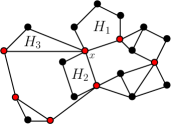
(a) $G$

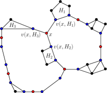
(b) $G^{\prime}$

Figure 1: Example construction of $G^{\prime}$ from $G$, as described in Proposition 2.

Let $S\subseteq V(G)$ such that every cycle of $G-S$ is contained in a $\mathcal{P}$-cluster of $G$. Towards a contradiction, suppose there is a cycle $C^{\prime}$ of $G^{\prime}-S$ containing at least one vertex $v\in X$. Note that $G$ can be obtained from $G^{\prime}$ by contracting each edge incident to a vertex $x\in X$, where the resulting vertex is labeled $x$. Thus, we can likewise obtain a cycle $C$ of $G-S$ by contracting each edge of $C^{\prime}$ incident with a vertex $x$ in $X$, labeling the resulting vertex $x$, and relabeling any remaining vertices not in $V(G)$ by their unique neighbor in $G^{\prime}$ that is a member of $X$. Suppose $v$ is adjacent to $u$ and $w$ in $C$. Then, by the construction of $G^{\prime}$, $u\in V(H)$ and $w\in V(H^{\prime})$ for distinct $\mathcal{P}$-clusters $H$ and $H^{\prime}$ of $G$. Clearly, $C$ is not contained in a $\mathcal{P}$-cluster of $G$ unless $u$ and $w$ are (not necessarily distinct) external vertices; but this implies that $H$ and $H^{\prime}$ share at least two vertices $u$ and $v$, contradicting the fact that $G$ is $\mathcal{P}$-clusterable. We deduce that no cycle of $G^{\prime}-S$ contains a vertex in $X$, as required.

Now let $S^{\prime}$ be a solution to Subset Feedback Vertex Set on $(G^{\prime},X,k)$. By the construction of $G^{\prime}$, each vertex in $V(G^{\prime})\setminus V(G)$ is adjacent to precisely one vertex in $X$. Let $U$ be the set of vertices in $X$ adjacent to a vertex in $S^{\prime}\setminus V(G)$ and set $S:=(S^{\prime}\cap V(G))\cup U$. Then $\lvert S\rvert\leqslant\lvert S^{\prime}\rvert$ and $S\subseteq V(G)$. We claim that every cycle of $G-S$ is contained in a $\mathcal{P}$-cluster. Suppose not; let $C$ be a cycle of $G-S$ not contained in a $\mathcal{P}$-cluster. Note that for each $v\in V(C)\cap X$, the vertex $v$ and its neighbors in $G^{\prime}$ are not in $S^{\prime}$. Thus, we obtain a cycle $C^{\prime}$ of $G^{\prime}-S^{\prime}$ from $C$ by performing one of the two following operations for each vertex $v\in V(C)\cap X$, where $u$ and $w$ are the two neighbors of $v$ in $C$:

1. If there is a $\mathcal{P}$-cluster $H$ of $G$ for which $\{u,v,w\}\subseteq V(H)$, then relabel $v$ in $C$ with the vertex in $V(G^{\prime})\setminus V(G)$ adjacent to $\{v\}\cup(N_{G}(v)\cap V(H))$.

2. Otherwise, for some $\mathcal{P}$-clusters $H_{1}$ and $H_{2}$ of $G$, we have that $u\in V(H_{1})\setminus V(H_{2})$, $v\in V(H_{1})\cap V(H_{2})$, and $w\in V(H_{2})\setminus V(H_{1})$. In this case, we subdivide $uv$ and $vw$ in $C$, labeling the new vertices $v_{1}$ and $v_{2}$ respectively, where $v_{i}$ is the vertex in $V(G^{\prime})\setminus V(G)$ adjacent to $\{v\}\cup(N_{G}(v)\cap V(H_{i}))$, for $i\in\{1,2\}$.

As $C$ is a cycle of $G-S$ not contained in a $\mathcal{P}$-cluster, at least one vertex $x$ in $V(C)\cap X$ has its neighbors in $C$ in distinct $\mathcal{P}$-clusters. By the second operation above, $x\in X$ is a vertex of $C^{\prime}$; a contradiction. We conclude that every cycle of $G-S$ is contained in a $\mathcal{P}$-cluster.

By Proposition 2, the $\mathcal{P}$-Block Vertex Deletion problem admits an efficient FPT algorithm provided we can reduce the input to $\mathcal{P}$-clusterable graphs. In the next section, we show that this is possible for any finite block-hereditary $\mathcal{P}$ where the permissible blocks in $\mathcal{P}$ have at most $d$ vertices. In particular, we use this to show there is an $\mathcal{O}^{*}(2^{\mathcal{O}(k\log d)})$-time algorithm for Bounded $\mathcal{P}$-Block Vertex Deletion.

3.2 An FPT Algorithm for Bounded $\mathcal{P}$-Block Vertex Deletion

In this section we describe an FPT algorithm for Bounded $\mathcal{P}$-Block Vertex Deletion using the clustering approach. For positive integers $x$ and $y$, let $\mathcal{B}_{x,y}$ be the class of all biconnected graphs with at least $x$ vertices and at most $y$ vertices. When $x>y$, $\mathcal{B}_{x,y}=\emptyset$.

Lemma 2

Let $\mathcal{P}$ be a non-degenerate block-hereditary class, and let $d\geqslant 2$ be an integer. If a graph $G$ is $\mathcal{B}_{d+1,2d-2}$-free and $(\mathcal{B}_{2,d}\setminus\mathcal{P})$-free, then $G$ is $(\mathcal{P}\cap\mathcal{B}_{2,d})$-clusterable.

Proof

Suppose $G$ has distinct $(\mathcal{P}\cap\mathcal{B}_{2,d})$-clusters $H_{1}$ and $H_{2}$ such that $|V(H_{1})\cap V(H_{2})|\geqslant 2$. Set $G^{\prime}:=G[V(H_{1})\cup V(H_{2})]$. By the maximality of $(\mathcal{P}\cap\mathcal{B}_{2,d})$-clusters, $V(H_{1})\setminus V(H_{2})$ and $V(H_{2})\setminus V(H_{1})$ are non-empty, so $|V(G^{\prime})|\geqslant 4$. The graph $G^{\prime}-v$ is connected for every $v\in V(G^{\prime})$, so $G^{\prime}$ is $2$-connected. Since $|V(G^{\prime})|\leqslant 2d-2$, but $G$ is $\mathcal{B}_{d+1,2d-2}$-free, $|V(G^{\prime})|\leqslant d$. Hence, by the maximality of $(\mathcal{P}\cap\mathcal{B}_{2,d})$-clusters, $G^{\prime}\notin\mathcal{P}$, which contradicts the fact that $G$ is $(\mathcal{B}_{2,d}\setminus\mathcal{P})$-free.

Proposition 3

Let $d\geqslant 2$ be an integer, and let $\mathcal{P}$ be a non-degenerate block-hereditary class recognizable in polynomial time. There is a polynomial-time algorithm that, given a graph $G$, either

1. outputs an induced subgraph of $G$ in $\mathcal{B}_{2,d}\setminus\mathcal{P}$, or

2. outputs an induced subgraph of $G$ in $\mathcal{B}_{d+1,2d-2}$, or

3. correctly answers that $G$ is $((\mathcal{B}_{2,d}\setminus\mathcal{P})\cup\mathcal{B}_{d+1,2d-2})$-free.

Proof

If $d\leqslant 2$, then (iii) holds trivially, so we may assume otherwise. We show that there is a polynomial-time algorithm FindObstruction that finds an induced subgraph of $G$ that is either in $\mathcal{B}_{2,d}\setminus\mathcal{P}$ or in $\mathcal{B}_{d+1,2d-2}$, if such an induced subgraph exists. For brevity, we refer to either type of induced subgraph as an obstruction. In the case that no obstruction exists, then $G$ is $(\mathcal{P}\cap\mathcal{B}_{2,d})$-clusterable, by Lemma 2.

First, we give an informal description of FindObstruction (Algorithm 1). We incrementally construct a biconnected induced subgraph $G[X]$, starting with $G[X]$ as the shortest cycle of $G$, by adding the vertices of a non-trivial $X$-path to $X$. If, at any increment, $G[X]$ is an obstruction, then we return $G[X]$. Otherwise, we eventually have that $G[X]$ is in $\mathcal{B}_{2,d}\cap\mathcal{P}$, but the union of $G[X]$ and any non-trivial $X$-path is not in $\mathcal{B}_{d+1,2d-2}$. Now, if there is a non-trivial $X$-path that together with a path in $G[X]$ forms a cycle of length at most $2d-2$, then this cycle is an obstruction, and we return it. Otherwise, no obstruction intersects $G[X]$ in any edges, so we remove the edges of $G[X]$ from consideration and repeat the process.

Algorithm 1 FindObstruction($G,d$)

1:Input: A graph $G$ and an integer $d>2$.

2:Output: An induced subgraph of $G$ that is either in $\mathcal{B}_{2,d}\setminus\mathcal{P}$ or in $\mathcal{B}_{d+1,2d-2}$; or No, if no such induced subgraph exists.

3:Set $\mathcal{H}:=\emptyset$.

4:while the shortest cycle in $G-\bigcup_{H\in\mathcal{H}}E(H)$ has length at most $2d-2$, do

5:     Set $G^{\prime}:=G-\bigcup_{H\in\mathcal{H}}E(H)$.

6:     Let $X$ be the vertex set of the shortest cycle in $G^{\prime}$.

7:     if $\lvert X\rvert\geqslant d+1$ or $G[X]\notin\mathcal{P}$ then

8:         return $G[X]$.

9:     end if$\triangleright$ $G[X]\in\mathcal{P}$ and $\lvert X\rvert\leqslant d$

10:     while there is a non-trivial $X$-path $P$ in $G^{\prime}$ such that $\lvert X\cup V(P)\rvert\leqslant d$, do

11:         Set $X:=X\cup V(P)$.

12:         if $G[X]\notin\mathcal{P}$ then

13:              return $G[X]$.

14:         end if

15:     end while $\triangleright$ $G[X]\in\mathcal{P}$ and $\lvert X\cup V(P)\rvert\geqslant d+1$ for any non-trivial $X$-path $P$

16:     if there is a non-trivial $X$-path $P$ in $G^{\prime}$ such that $\lvert X\cup V(P)\rvert\leqslant 2d-2$, then

17:         return $G[X\cup V(P)]$.

18:     else if for some distinct $u,v\in X$, there is a $uv$-path $P$ in $G[X]$ and a $uv$-path $P^{\prime}$ in $G^{\prime}-E(G[X])$ with $l(P)+l(P^{\prime})\leqslant 2d-2$, then

19:         return $G[V(P)\cup V(P^{\prime})]$.

20:     end if$\triangleright$ No obstruction meets $E(G[X])$

21:     Add $G[X]$ to $\mathcal{H}$.

22:end while

23:return No.

Now we prove the correctness of the algorithm. Since $\mathcal{P}$ is non-degenerate, $K_{2}$ is not an obstruction.

Consider an induced subgraph $H:=G[X]$ added to $\mathcal{H}$ at line 21. As the edges of $H$ are excluded in future iterations, we will show that these edges do not meet the edges of any obstruction. That is, we claim that for every $Y\subseteq V(G)$ such that $G[Y]$ is an obstruction, $E(H)\cap E(G[Y])=\emptyset$. Towards a contradiction, suppose $G[Y]$ is an obstruction for some $Y\subseteq V(G)$, and $uv\in E(H)\cap E(G[Y])$. Clearly $\lvert X\rvert\leqslant d$, and $G[X]\in\mathcal{P}$. Note also that $Y\nsubseteq X$, since $\lvert Y\rvert\leqslant d$ implies that $G[Y]\notin\mathcal{P}$, but $G[X]\in\mathcal{P}$. Since $G[Y]$ is biconnected and not isomorphic to $K_{2}$, it has a cycle subgraph $C$ that contains the edge $uv$. Let $P$ be a non-trivial $X$-path in $C$. Since there is a path in $H$ of length at most $d-1$ between any two distinct vertices in $X$, it follows that $P$ has length more than $d-1$, otherwise there is a path satisfying the conditions of line 18. Since $\lvert Y\rvert\leqslant 2d-2$, we deduce that there are no two distinct $X$-paths in $C$. So $C$ is the union of $P$ and a path contained in $H$. Thus $P$ is a $uv$-path satisfying the conditions of line 18; a contradiction. This verifies our claim.

Now we show that if $G$ contains an obstruction, then the algorithm outputs an obstruction. Suppose that $G$ contains an induced subgraph $J\in(\mathcal{B}_{2,d}\setminus\mathcal{P})\cup\mathcal{B}_{d+1,2d-2}$. Since $\lvert V(J)\rvert\leqslant 2d-2$ and $J$ is biconnected, but not isomorphic to $K_{2}$, it contains a cycle of length at most $2d-2$. So execution reaches line 4 and, from the previous paragraph, $J$ is a subgraph of in $G^{\prime}$ as given in line 5. It is clear that the flow of execution will reach line 8, line 13, line 17, line 19, or line 21. Clearly, a graph returned at line 8 is an obstruction. A graph returned at either line 13 or line 17 is $2$-connected, since it has an obvious open ear decomposition (see, for example, [2, Theorem 5.8]), and thus is easily seen to be an obstruction. If a graph is returned at line 19, it is a cycle, and since $l(P^{\prime})\geqslant d$, such a graph is also in $\mathcal{B}_{d+1,2d-2}$. By the previous paragraph, if execution reaches line 21, then $E(G[X])$ does not meet $E(J)$, so execution will loop, with $\lvert E(G^{\prime})\rvert$ strictly smaller in the following iteration. Thus, eventually the algorithm will find either $J$, or another obstruction.

It remains to prove that the algorithm runs in polynomial time. We observe that there will be at most $\mathcal{O}(m)$ loops of the outer ‘while’ block, and at most $\mathcal{O}(m)$ loops of the inner ‘while’ block. Finding a shortest cycle, or all shortest $X$-paths for some $X\subseteq V(G)$, takes time $\mathcal{O}(n^{3})$ by the Floyd-Warshall algorithm. It follows that the algorithm runs in polynomial time.

Lemma 3

Let $d\geqslant 2$ be an integer, and let $\mathcal{P}$ be a non-degenerate block-hereditary class recognizable in polynomial time. Then there is a polynomial-time algorithm that, given a $((\mathcal{B}_{2,d}\setminus\mathcal{P})\cup\mathcal{B}_{d+1,2d-2})$-free graph $G$, outputs the set of $(\mathcal{P}\cap\mathcal{B}_{2,d})$-clusters of $G$.

Proof

Let $\mathcal{P}^{\prime}=\mathcal{P}\cap\mathcal{B}_{2,d}$. By Proposition 3, $G$ is $\mathcal{P}^{\prime}$-clusterable. We argue that the algorithm Cluster (Algorithm 2) meets the requirements of the lemma.

Algorithm 2 Cluster($G$)

1:Input: A $(\mathcal{B}_{2,d}\setminus\mathcal{P})$-free $\mathcal{P}^{\prime}$-clusterable graph $G$.

2:Output: The set $\mathcal{H}$ of $\mathcal{P}^{\prime}$-clusters of $G$.

3:Set $\mathcal{H}:=\emptyset$ and $G^{\prime}:=G$.

4:while the shortest cycle in $G^{\prime}$ has length at most $d$, do

5:     Let $X$ be the vertex set of the shortest cycle in $G^{\prime}$. $\triangleright$ $G[X]\in\mathcal{P}$

6:     while there is a non-trivial $X$-path $P$ in $G^{\prime}$ such that $\lvert X\cup V(P)\rvert\leqslant d$, do

7:         Set $X:=X\cup V(P)$. $\triangleright$ $G[X]\in\mathcal{P}$

8:     end while$\triangleright$ No obstruction meets $E(G[X])$

9:     Add $G[X]$ to $\mathcal{H}$.

10:     Set $G^{\prime}:=G^{\prime}-E(G[X])$.

11:end while

12:if $G^{\prime}$ is edgeless, then

13:     return $\mathcal{H}$.

14:else

15:     return $\mathcal{H}\cup\{G^{\prime}[\{x,y\}]:\text{$x$ and $y$ are adjacent in $G^{\prime}$}\}$.

16:end if

It is clear that this algorithm runs in polynomial time. We now prove correctness of the algorithm. A graph $G[X]$ at line 5 or line 7 is $2$-connected, since it has an obvious open ear decomposition, and in $\mathcal{P}$, since $G$ is $(\mathcal{B}_{2,d}\setminus\mathcal{P})$-free. By line 9, the graph $G[X]$ has the property that, for any non-trivial $G[X]$ path $P$, $|X\cup V(P)|>d$. So any $2$-connected graph containing $G[X]$ as a proper subgraph consists of at least $d+1$ vertices, and hence is not in $\mathcal{P}^{\prime}$. This proves that $G[X]$ is indeed a $\mathcal{P}^{\prime}$-cluster. Since $G$ is $\mathcal{P}^{\prime}$-clusterable, any $\mathcal{P}^{\prime}$-cluster distinct from $G[X]$ does not share any edges with $G[X]$, so we can safely remove them from consideration, and repeat this procedure. If $G$ contains no cycles of length at most $d$, then the only remaining biconnected components are isomorphic to $K_{1}$ or $K_{2}$.

Theorem 3.1

Let $\mathcal{P}$ be a non-degenerate block-hereditary class of graphs recognizable in polynomial time. Then Bounded $\mathcal{P}$-Block Vertex Deletion can be solved in time $2^{\mathcal{O}(k\log d)}n^{\mathcal{O}(1)}$.

Proof

We describe a branching algorithm for Bounded $\mathcal{P}$-Block Vertex Deletion on the instance $(G,d,k)$. If $G$ contains an induced subgraph in $(\mathcal{B}_{2,d}\setminus\mathcal{P})\cup\mathcal{B}_{d+1,2d-2}$, then any solution $S$ contains at least one vertex of this induced subgraph. We first run the algorithm of Proposition 3, and if it outputs such an induced subgraph $J$, then we branch on each vertex $v\in V(J)$, recursively applying the algorithm on $(G-v,d,k-1)$. Since $\lvert V(J)\rvert\leqslant 2d-2$, there are at most $2d-2$ branches. If one of these branches has a solution $S^{\prime}$, then $S^{\prime}\cup\{v\}$ is a solution for $G$. Otherwise, if every branch returns No, we return that $(G,d,k)$ is a No-instance. On the other hand, if there is no such induced subgraph, then $G$ is $(\mathcal{P}\cap\mathcal{B}_{2,d})$-clusterable, by Lemma 2, and we can find the set of all $(\mathcal{P}\cap\mathcal{B}_{2,d})$-clusters in polynomial time, by Lemma 3. We can now run the $\mathcal{O}^{*}(4^{k})$-time algorithm of Proposition 2 and return the result. Thus, an upper bound for the running time is given by the following recurrence:

$$T(n,k)=\begin{cases}1&\text{if $k=0$ or $n=0$,}\\ 4^{k}n^{\mathcal{O}(1)}&\text{if $((\mathcal{B}_{2,d}\setminus\mathcal{P})\cup\mathcal{B}_{d+1,2d-2})$-free,}\\ (2d-2)T(n-1,k-1)+n^{\mathcal{O}(1)}&\text{otherwise.}\\ \end{cases}$$

Hence, we have an algorithm that runs in time $\mathcal{O}^{*}(2^{\mathcal{O}(k\log d)})$.

4 Bounded $\mathcal{P}$-Block Vertex Deletion Lower Bounds

4.1 A Tight Lower Bound

The Exponential-Time Hypothesis (ETH), formulated by Impagliazzo, Paturi, and Zane [10], implies that $n$-variable 3-SAT cannot be solved in time $2^{o(n)}$. We now argue that the previous algorithm is essentially tight under the ETH.

The $k\nobreak\times\nobreak k$ Clique problem takes as input an integer $k$ and a graph on $k^{2}$ vertices, each vertex corresponding to a distinct point of a $k$ by $k$ grid, and asks for a clique of size $k$ hitting each column of the grid exactly once. Unless the ETH fails, $k\nobreak\times\nobreak k$ Clique is not solvable in time $2^{o(k\log k)}$ [17]. However, solving Bounded $\mathcal{P}$-Block Vertex Deletion in $2^{o(k\log d)}$ time, where $\mathcal{P}$ contains all biconnected split graphs, implies that $k\nobreak\times\nobreak k$ Clique can be solved in $2^{o(k\log k)}$ time.

See 1.2

Proof

In [6], the authors show that Component Order Connectivity cannot be solved in $2^{o(k\log d)}$ time unless the ETH fails. We adapt their reduction from $k\nobreak\times\nobreak k$ Clique. We recall that a split graph is a graph whose vertex set can be partitioned into two sets, one inducing a clique and the other inducing an independent set. Let $(G,k)$ be an instance of $k\nobreak\times\nobreak k$ Clique. Since the edges between vertices in the same column cannot be involved in a solution, we may assume that each column induces an independent set. Then $(G,k)$ is a Yes-instance if and only if $G$ has a $k$-clique. We build an instance $(G^{\prime},d,k^{\prime})$ of Bounded $\mathcal{P}$-Block Vertex Deletion where $V(G^{\prime})=Q\cup I$ for $Q=V(G)\cup E_{1}$ and $I=E_{2}$, where $E_{1}$ and $E_{2}$ are two copies of $E(G)$. For each edge $e\in E(G)$, we denote by $e^{1}$ (resp. $e^{2}$) the corresponding vertex in $E_{1}$ (resp. in $E_{2}$). The set $Q$ induces a clique while $I$ induces an independent set. For each edge $e=uv\in E(G)$, we add three edges $ue^{2}$, $ve^{2}$ and $e^{1}e^{2}$ in $G^{\prime}$, each between a vertex in $Q$ and a vertex in $I$. This ends the construction of $G^{\prime}$. Observe that $G^{\prime}$ is a split graph and the vertices in $I$ all have degree $3$. We set $k^{\prime}:=k$ and $d:=|V(G^{\prime})|-k-{k\choose 2}$. Note that $|V(G^{\prime})|\geqslant|V(G)|=k^{2}$, so $d\geqslant k^{2}-k-{k\choose 2}={k\choose 2}$. Without loss of generality we may assume that $k\geqslant 3$, and hence $d\geqslant 2$.

Assume that $G$ admits a $k$-clique $S=\{v_{1},\ldots,v_{k}\}$, and denote $v_{i}v_{j}$ by $e_{ij}$. We claim that $S$ is a solution for Bounded $\mathcal{P}$-Block Vertex Deletion on the instance $(G^{\prime},d,k^{\prime})$. Indeed, for each of the ${k\choose 2}$ pairs $(i,j)$ with $i<j\in[k]$, the vertex $e_{ij}^{2}$ has degree $1$ in $G^{\prime}-S$, so its unique neighbor, $e_{ij}^{1}$, is a cut vertex. Hence, $e_{ij}^{2}$ is not in the block containing the clique $Q\setminus S$. Therefore, the blocks of $G^{\prime}-S$ have at most $|V(G^{\prime})|-k-{k\choose 2}$ vertices.

We now assume that there is a set $S\subseteq V(G^{\prime})$ of at most $k$ vertices such that all the blocks of $G^{\prime}-S$ have at most $d$ vertices. We call the main block the one containing $Q\setminus S$. The only vertices of $G^{\prime}-S$ that are not in the main block are the vertices $X$ of $I$ with degree at most $1$ in $G^{\prime}-S$. Since the main block has at most $d$ vertices, there are at least ${k\choose 2}$ vertices in $X$. This implies that $X$ corresponds to the ${k\choose 2}$ edges of a $k$-clique in $G$.

Since $|V(G)|=k^{2}$, we have that $|E(G)|=\mathcal{O}(k^{4})$. Thus $d=\mathcal{O}(k^{4})$ and $\log d=\mathcal{O}(\log k)$. Therefore, solving Bounded $\mathcal{P}$-Block Vertex Deletion in $2^{o(k\log d)}$ time would also solve $k\nobreak\times\nobreak k$ Clique in time $2^{o(k\log k)}$, contradicting the ETH.

4.2 $W[1]$-hardness Parameterized Only by $k$

We now prove that Bounded $\mathcal{P}$-Block Vertex Deletion is $W[1]$-hard when parameterized only by $k$, if $\mathcal{P}$ is a class such that $\Phi_{\mathcal{P}}$ contains all split graphs. In particular, this implies that Bounded Block VD is $W[1]$-hard when parameterized only by $k$. The reduction is similar to that in Section 4.1, but the reduction is from Clique, rather than $k\nobreak\times\nobreak k$ Clique.

See 1

Proof

Consider an instance $(G,k)$ of the problem Clique where, given a graph $G$ and integer $k$, the question is whether $G$ has a $k$-clique. Observe that we can perform the same reduction given in the proof of Theorem 1.2 but from Clique, rather than $k\nobreak\times\nobreak k$ Clique. By doing so, we build an instance $(G^{\prime},d,k)$ of Bounded $\mathcal{P}$-Block Vertex Deletion where $G^{\prime}$ is a split graph, and for which $S$ is a solution for the instance $(G^{\prime},d,k)$ if and only if $S$ is a $k$-clique of $G$. Since the reduction is parameter preserving, the result then follows from the fact that Clique is $W[1]$-hard when parameterized by the size of the solution [5].

5 $\mathcal{O}^{*}(c^{k})$-time Algorithms Using Iterative Compression

We now consider the specializations of Bounded $\mathcal{P}$-Block Vertex Deletion that we refer to as Bounded Complete Block VD and Bounded Cactus Graph VD. These problems are “bounded” variants of Complete Block Vertex Deletion and Diamond Hitting Set, respectively, which are known to admit $c^{k}n^{\mathcal{O}(1)}$ fixed-parameter tractable algorithms for some constant $c$. By Theorem 3.1, Bounded Complete Block VD and Bounded Cactus Graph VD can be solved in $\mathcal{O}^{*}(2^{\mathcal{O}(k\log d)})$ time. However, the next two theorems show that these problems are in fact FPT parameterized only by $k$, and, like their “unbounded” variants, each has a $c^{k}n^{\mathcal{O}(1)}$-time algorithm. The proofs of these results use the well-known technique of iterative compression [19], which we now briefly recap.

In a nutshell, the idea of iterative compression is to try and build a solution of size $k$ given a solution of size $k+1$. It is typically used for graph problems where one wants to remove a set $S$ of at most $k$ vertices such that the resulting graph satisfies some property or belongs to some class. We call such a set $S$ a solution or a deletion set. Say $S$ is a solution of size $k+1$ for a problem $\Pi$ on a graph $G$ that we want to compress into a solution $R$ of size at most $k$. We can try out all $2^{k+1}$ possible intersections of old and new solutions $I=S\cap R$. In each case, we remove $I$ from $G$ and look for a solution of size at most $k-|I|$ that does not intersect $S\setminus I$. We call Disjoint $\Pi$ this new problem of finding a solution of size at most $k$ that does not intersect a given deletion set $S$ of size up to $k+1$. If we can solve Disjoint $\Pi$ in time $\mathcal{O}^{*}(c^{k})$, then the running time of this approach to solve $\Pi$ is $\mathcal{O}^{*}(\Sigma_{i=0}^{k+1}{k+1\choose i}c^{k-i})=\mathcal{O}^{*}((c+1)^{k})$. We can start with a subgraph of $G$ induced by any set of $k+1$ vertices. Those $k+1$ vertices constitute a trivial deletion set. After one compression step, we obtain a solution of size $k$. Then, a new vertex is added to the graph and immediately added to the deletion set. We compress again, and so on. After a linear number of compressions, we have added all the vertices of $G$, so we have a solution for $G$. For more about iterative compression, we refer the reader to Cygan et al. [4], or Downey and Fellows [5].

5.1 Bounded Complete Block VD

See 1.3

Proof

It is sufficient to solve Disjoint Bounded Complete Block VD in time $\mathcal{O}^{*}(9^{k})$. Let $(G,S,d,k)$ be an instance where $S$ is a deletion set of size $k+1$. We present an algorithm that either finds a solution $R$ of size at most $k$ not intersecting $S$, or establishes that there is no such solution. For convenience, $G$, $S$, and $R$ are not fixed objects; they represent, respectively, the remaining graph, the set of vertices that we cannot delete, and the solution that is being built, throughout the execution of the algorithm. Initially, $R$ is empty. For an instance $I=(G,S,d,k)$, we take as a measure $\mu(I)=k+\text{cc}(S)$, where $\text{cc}(S)$ is the number of connected components of $G[S]$. Thus, $\mu(I)\leqslant 2k+1$. We say a graph $G$ is a $d$-complete block graph if every block of $G$ is a clique of size at most $d$. We present two reduction rules and three branching rules that we apply while possible.

Reduction Rule 5.1

If there is a vertex $u\in V(G)\setminus S$ with degree at most $1$ in $G$, then we remove $u$ from $G$.

The soundness of this rule is straightforward.

Reduction Rule 5.2

If there is a vertex $u\in V(G)\setminus S$ such that $G[S\cup\{u\}]$ is not a $d$-complete block graph, then remove $v$ from $G$, put $v$ in $R$, and decrease $k$ by $1$.

This reduction rule is safe since any induced subgraph of a $d$-complete block graph is itself a $d$-complete block graph. Here, an obstruction is a $2$-connected induced subgraph that is not a clique of size at most $d$. At least one vertex of any obstruction should be in a solution. We can restate the rule as follows: if a vertex $u\in V(G)\setminus S$ forms an obstruction with vertices of $S$, then $u$ is in any solution. We also observe that if a graph contains no obstruction, then it is a $d$-complete block graph.

Branching Rule 5.1

If there are distinct vertices $u$ and $v$ in $G-S$ such that $G[S\cup\{u,v\}]$ is not a $d$-complete block graph, then branch on either removing $u$ from $G$, putting $u$ in $R$, and decreasing $k$ by $1$; or removing $v$ from $G$, putting $v$ in $R$, and decreasing $k$ by $1$.

This branching rule is exhaustive since at least one of $u$ and $v$ has to be in $R$, as $G[S\cup\{u,v\}]$ contains an obstruction. In both subinstances $\mu(I)$ is decreased by $1$, so the associated branching vector for this rule is $(1,1)$.

Branching Rule 5.2

If there is a vertex $u\in V(G)\setminus S$ having two neighbors $v,w\in S$ such that $v$ and $w$ are in distinct connected components of $G[S]$, then branch on either removing $u$ from $G$, putting $u$ in $R$, and decreasing $k$ by $1$; or adding $u$ to $S$.

If $u$ is added to $S$, then the number of connected components in $G[S]$ decreases by at least $1$. This branching rule is exhaustive and in both cases $\mu(I)$ is decreased by at least $1$, so the associated branching vector is $(1,1)$.

Branching Rule 5.3

Suppose there is an edge $uv$ of $G-S$ such that $u$ has a neighbor $u^{\prime}\in S$ and $v$ has a neighbor $v^{\prime}\in S$, and $u^{\prime}$ and $v^{\prime}$ are in distinct connected components of $G[S]$. We branch on three subinstances:

1. remove $u$ from the graph, put it in $R$, and decrease $k$ by $1$,

2. remove $v$ from the graph, put it in $R$, and decrease $k$ by $1$, or

3. put both $u$ and $v$ in the set $S$.

Again, this branching rule is exhaustive: either $u$ or $v$ is in the solution $R$, or they can both be safely put in $S$. In branch (c), the number of connected components of $G[S]$ decreases by at least $1$. Therefore, the associated branching vector for this rule is $(1,1,1)$.

Applying the two reduction rules and the three branching rules presented above preserves the property that $G-S$ is a $d$-complete block graph. The algorithm first applies these rules exhaustively (see Algorithm 3), so we now assume that we can no longer apply these rules.

Let $x$ be a vertex $V(G)\setminus S$ and consider its neighborhood in $S$. We claim that this neighborhood is either empty, a single vertex, or all the vertices of some block of $G[S]$. Suppose $x$ has at least two neighbors $y$ and $z$ in $S$. Then, since Branching Rule 5.2 cannot be applied, $y$ and $z$ are in the same connected component of $G[S]$. Now, if no block of $G[S]$ contains both $y$ and $z$, then $x$ forms an obstruction with vertices in $S$, contradicting the fact that Reduction Rule 5.2 cannot be applied. It follows that the vertices of the block containing $y$ and $z$, together with $x$, form a clique. Moreover, $x$ has no other neighbors. This proves the claim.

Let $C$ be the vertex set of a leaf block of $G-S$. We know that $C$ is a clique of size at most $d$, and the block $G[C]$ of $G-S$ has at most one cut vertex. If the block $G[C]$ of $G-S$ has a cut vertex $v$, let $C^{\prime}:=C\setminus\{v\}$; otherwise, let $C^{\prime}:=C$. We use this notation in all the remaining reduction and branching rules. The next three rules handle the case where at most one vertex in $C$ has neighbors in $S$.

Reduction Rule 5.3

If none of the vertices in $C^{\prime}$ have neighbors in $S$, then remove $C^{\prime}$ from $G$.

If the block $G[C]$ of $G-S$ does not have a cut vertex, then $C^{\prime}$ is a connected component of $G$, so we obtain an equivalent instance after removing $C^{\prime}$ from $G$. If the block $G[C]$ of $G-S$ has a cut vertex $v$, then either $v$ is in the solution $R$, and $C^{\prime}$ is a clique of size at most $d$ that is a connected component of $G-R$; or $v$ is in the $d$-complete block graph $G-R$, and $G[C]$ is a leaf block of this graph. In either case, no vertex in $C^{\prime}$ can be in an obstruction. Each vertex not in any obstruction can be removed from $G$ without changing the value of $k$.

The soundness of the next rule follows from a similar argument.

Reduction Rule 5.4

If the block $G[C]$ of $G-S$ does not have a cut vertex, $w\in C$ has at least one neighbor in $S$, and each vertex in $C\setminus\{w\}$ has no neighbor in $S$, then put $C$ in $S$.

Reduction Rule 5.5

If the block $G[C]$ of $G-S$ has a cut vertex, $w\in C^{\prime}$ has at least one neighbor in $S$, and each vertex in $C\setminus\{w\}$ has no neighbor in $S$, then put $w$ in $S$.

In order to show that this rule is sound, we now prove that if $R$ is a solution containing $w$, then $(R\setminus\{w\})\cup\{v\}$ is also a solution. Since Reduction Rule 5.2 cannot be applied, $w$ together with its neighborhood in $S$ forms a maximal clique in $G$, and this clique consists of at most $d$ vertices. Suppose $R\setminus\{w\}$ is not a solution. Then $G-(R\setminus\{w\})$ contains some obstruction, and any such obstruction contains $w$. Since $w$ is not contained in a clique of size more than $d$ in $G$, every minimal obstruction is either a diamond or an induced cycle. Since Branching Rule 5.1 cannot be applied, $w$ is not contained in an induced diamond subgraph of $G$. But every induced cycle containing $w$ and not contained in $S\cup\{w\}$ must contain $v$, which proves the claim.

Now, we consider the case where at least two vertices in $C$ each have at least one neighbor in $S$. Let $x$ and $y$ be two such vertices. We claim that $x$ and $y$ have the same neighborhood in $S$. Since $C$ is a clique, $x$ and $y$ are adjacent. As Branching Rule 5.3 does not apply, the neighbors of $x$ and $y$ in $S$ are all in the same component of $G[S]$. Now, if the neighborhoods of $x$ and $y$ differ, then $G[S\cup\{x,y\}]$ contains an obstruction, so Branching Rule 5.1 can be applied; a contradiction. This proves the claim.

Thus, $C$ can be partitioned into $C_{1}\cup C_{2}$ where the vertices of $C_{1}$ all share the same non-empty neighborhood in $S$, while the vertices of $C_{2}$ have no neighbor in $S$. The previous three reduction rules handled the case where $|C_{1}|\leqslant 1$. We now handle the case where $|C_{1}|\geqslant 2$.

Reduction Rule 5.6

If all the vertices of $C$ have the same non-empty neighborhood $A$ in $S$ (that is, $C_{2}=\emptyset$), then remove any $s:=\max\{0,\lvert C^{\prime}\rvert-d+\lvert A\rvert\}$ vertices of $C^{\prime}$ from $G$, put them in $R$, decrease $k$ by $s$, and put the remaining vertices of $C^{\prime}$ in $S$.

Firstly, note that if $C$ contains a cut vertex $v$ and $|C\cup A|\leqslant d$, it is always better to have $v$ in $R$ rather than a vertex of $C^{\prime}$. So, in this case, we can safely add the vertices of $C^{\prime}$ to $S$, and, after doing so, $G[S]$ is still a $d$-complete block graph. However, when $|C\cup A|>d$, we have to put some vertices of $C^{\prime}$ in $R$, since $C\cup A$ is a clique. As these vertices are twins (that is, they have the same closed neighborhood), it does not matter which $s$ vertices of $C^{\prime}$ we choose.

In the final case, where $|C_{1}|\geqslant 2$ and $|C_{2}|\geqslant 1$, we use the following branching rule:

Branching Rule 5.4

Suppose there are at least two vertices of $C$ having the same non-empty neighborhood in $S$ (that is, $|C_{1}|\geqslant 2$) and at least one vertex of $S$ having no neighbor in $S$ (that is, $|C_{2}|\geqslant 1$). We branch on two subinstances:

1. remove all the vertices of $C_{2}$ from $G$, put them in $R$, and decrease $k$ by $|C_{2}|$, or

2. choose any vertex $x\in C_{1}\cap C^{\prime}$, then remove all the vertices of $C_{1}\setminus\{x\}$, put them in $R$, and decrease $k$ by $|C_{1}|-1$.

We now argue that this branching rule is sound. Let $x$ and $y$ be distinct vertices in $C_{1}$, and let $z$ be in $C_{2}$. Then, for any common neighbor $t\in S$ of $x$ and $y$, the set $\{t,x,y,z\}$ induces a diamond in $G$, which is an obstruction. In order to eliminate all such obstructions, we must remove vertices from $G$ so that either $C_{2}$ is empty, as in (a), or $\lvert C_{1}\rvert\leqslant 1$, as in (b). In case (b), we can safely pick $x\in C^{\prime}$ as the vertex not added to $R$ since it is always preferable to add a cut vertex of $G-S$ in $C$ to $R$, rather than a vertex in $C^{\prime}$. In either subinstance, the measure is decreased by at least $1$, so the associated branching vector is $(1,1)$.

Algorithm 3 Disjoint-BoundedCompleteBlockVD($G,S,d,k$)

1:Input: A graph $G$, a subset of vertices $S$, and two integers $d$ and $k$.

2:Output: A set $R$ of size at most $k$ such that $R\cap S=\emptyset$ and $G-R$ is a $d$-complete block graph.

3:Set $R:=\emptyset$.

4:while $k\geqslant 0$ and $G-S$ is non-empty do

5:     if Reduction Rules 5.1 and 5.2 or one of Branching Rules 5.1, 5.2 and 5.3 can be applied then

6:         Apply this rule

7:     else

8:         Apply one of Reduction Rules 5.3, 5.4, 5.5 and 5.6, or Branching Rule 5.4

9:     end if

10:end while

11:if $k\geqslant 0$ then

12:     return $R$.

13:end if

Once we apply one rule among Reduction Rules 5.3, 5.4, 5.5, 5.6 and 5.4, we check whether or not the first set of rules can be applied again (see Algorithm 3).

The algorithm ends when $G-S$ is empty, or if $k$ becomes negative, in which case there is no solution at this node of the branching tree. Indeed, while $G-S$ has at least one vertex, there is always some rule to apply. When $G-S$ is empty, $R$ is a solution for $(G,S,d,k)$. Each reduction rule can only be applied a linear number of times since they all remove at least one vertex from $G$. Thus, the overall running time is bounded above by the slowest branching, namely the one with the branching vector $(1,1,1)$, for which the running time is $\mathcal{O}^{*}(3^{\mu(I)})=\mathcal{O}^{*}(9^{k})$.

5.2 Bounded Cactus Graph VD

See 1.4

Proof

As in the proof of Theorem 1.3, it suffices to solve Disjoint Bounded Cactus Graph VD in time $\mathcal{O}^{*}(25^{k})$.

For a positive integer $d$, we say a $d$-cactus is a graph where each block containing at least two vertices is either a cycle of length at most $d$ or an edge ($d$-cactus graphs are a subclass of cactus graphs). Similarly to Disjoint Bounded Complete Block VD, we take as a measure $\mu(I)=k+\text{cc}(S)$ for an instance $I=(G,S,d,k)$, we denote by $R$ the solution that we build, and an obstruction is a $2$-connected induced subgraph that is not a cycle of size at most $d$. As all the vertices of $S$ will be in the graph $G-R$, there can only be a solution to Disjoint Bounded Cactus Graph VD if $G[S]$ is a $d$-cactus. Indeed, observe that any induced subgraph of a $d$-cactus is itself a $d$-cactus. We now assume that $G[S]$ is a $d$-cactus. As $S$ is a solution, $G-S$ is also a $d$-cactus. We will preserve the property that the blocks of both $G[S]$ and $G[V(G)\setminus S]$ are either cycles of length at most $d$, or consist of a single edge.

We begin by applying the following four rules while possible. The first two of these are Reduction Rules 5.1 and 5.2. Recall that this latter branching rule is exhaustive, and its associated branching vector is $(1,1)$ for the measure $\mu$.

Reduction Rule 5.7

If there is a vertex $u\in V(G)\setminus S$ such that $G[S\cup\{u\}]$ is not a $d$-cactus, then remove $u$ from the graph, put $u$ in $R$, and decrease $k$ by $1$.

Again, this rule is sound since any induced subgraph of a $d$-cactus is a $d$-cactus.

We define a red vertex as a vertex of $V(G)\setminus S$ that has at least one neighbor in $S$. We say that two distinct red vertices are consecutive red vertices if they are both contained in some block of $G-S$ and there is a path between them in which all the internal vertices have degree $2$ in $G$. Let $a$ and $b$ be vertices that are either red, or of degree at least $3$, or in $S$, with the additional constraint that $a$ and $b$ are not both in $S$. A chain from $a$ to $b$, or simply a chain, is the set of internal vertices, all of degree $2$, of a path between $a$ and $b$.

Branching Rule 5.5

Suppose $v$ and $w$ are consecutive red vertices in a block of $G-S$, where $s\in S$ is a neighbor of $v$, the vertex $t\in S$ is a neighbor of $w$, and $s$ and $t$ are in distinct connected components of $G[S]$. Then, either

1. remove $v$ from $G$, put $v$ in $R$, and decrease $k$ by $1$; or

2. remove $w$ from $G$, put $w$ in $R$, and decrease $k$ by $1$; or

3. put $\{v,w\}\cup P$ in $S$, where $P$ is a chain from $v$ to $w$.

This branching rule is safe since for any solution $R^{\prime}$ that does not contain $v$ nor $w$ but contains a vertex $z$ of the chain $P$, the set $(R^{\prime}\setminus\{z\})\cup\{v\}$ is also a solution. As we use this observation several times, we state it as a lemma.

Lemma 4

If there is a solution, then there is one that does not contain any vertex of a chain.

Proof

In any solution, we may replace a vertex in a chain $P$ by the (at least) one vertex not in $S$ among the two vertices in the open neighborhood of $P$.

The branching vector of Branching Rule 5.5 is $(1,1,1)$ since in the first two cases $k$ decreases by $1$, and in the third $\text{cc}(S)$ decreases by $1$.

Whenever these four rules cannot be applied, we claim that:

1. every vertex of $V(G)\setminus S$ has degree at most $2$ in $S$, and

2. the neighborhood in $S$ of the set of red vertices in a block is contained in some connected component of $G[S]$.

Indeed, since Branching Rule 5.2 is not applicable, a vertex $w$ of $V(G)\setminus S$ has neighbors in at most one connected component in $G[S]$. Now, suppose $w$ has at least three neighbors $a$, $b$, and $c$ in the same connected component. Then $waP_{1}bw$ and $wbP_{2}cw$, where $P_{1}$ is an $ab$-path in $G[S]$ and $P_{2}$ is a $bc$-path in $G[S]$, are distinct cycles that intersect on at least $w$ and $b$. Hence, Reduction Rule 5.7 applies for $w$; a contradiction. Finally, we see that (2) holds because otherwise Branching Rule 5.5 would apply.

Now, we assume that the first four rules do not apply (see Algorithm 4).

Branching Rule 5.6

Let $u$, $v$, and $w$ be distinct vertices of a block of $G-S$. If $u$ and $v$ are consecutive red vertices, and $v$ and $w$ are consecutive red vertices, then branch on putting either $u$, or $v$, or $w$ into the solution $R$. In each case, remove the vertex from $G$ and decrease $k$ by $1$.

By (2), the neighbors in $S$ of $u$, $v$ and $w$ are in the same connected component of $G[S]$. Therefore, a set consisting of $u$, $v$, $w$, the two chains from $u$ and $v$ and from $v$ and $w$, and $S$ induces a graph that contains a subdivision of a diamond, hence is an obstruction. By Lemma 4, we conclude that branching on the three red vertices $u$, $v$, and $w$ is safe. The branching vector is again $(1,1,1)$.

We now deal with leaf blocks in $G-S$ that consist of a single edge. We call such a block a leaf edge.

Reduction Rule 5.8

Suppose $uv$ is a leaf edge in $G-S$ where $u$ is a red vertex of degree $1$ in $S$, and $v$ is either a cut vertex of $G-S$ or a red vertex of degree $1$ in $S$. Then, put $u$ in $S$.

If $v$ is a cut vertex, then this rule is safe by Lemma 4 since $\{u\}$ is a chain. Otherwise, for any solution $R^{\prime}$ containing $u$, the set $(R^{\prime}\setminus\{u\})\cup\{v\}$ is also a solution.

Branching Rule 5.7

Suppose $uv$ is a leaf edge in $G-S$, where $u$ and $v$ are red vertices, and $u$ has two neighbors in $S$. Then, branch on putting either $u$ or $v$ into the solution $R$. In either case, remove the vertex from $G$ and decrease $k$ by $1$.

By (2), $G[S\cup\{u,v\}]$ contains an obstruction, so this rule is safe. The branching vector is $(1,1)$.

When these rules have been applied exhaustively, we claim that

1. each block of $G-S$ contains at most two red vertices, and

2. each leaf edge of $G-S$ has one red vertex, and this vertex is not a cut vertex of $G-S$, and has degree $2$ in $S$.

The first claim follows immediately from the fact that Branching Rule 5.6 cannot be applied. Now suppose $G-S$ has a leaf edge consisting of vertices $u$ and $v$. Since Reduction Rule 5.1 cannot be applied, $u$ and $v$ are either both red, or one is red and the other is a cut vertex of $G-S$. If they are both red, then either Branching Rule 5.7 can be applied, if $u$ or $v$ has degree at least $2$ in $S$, or Reduction Rule 5.8 can be applied, if $u$ and $v$ both have degree $1$ in $S$; a contradiction. So we may assume that only $u$ is red, and $v$ is a cut vertex of $G-S$. In this case, by (1) and since Reduction Rule 5.8 cannot be applied, $u$ has degree $2$ in $S$.

Now, we apply one of the following three rules, if possible.

Branching Rule 5.8

Suppose $u$ and $v$ are distinct (consecutive) red vertices in a leaf block that is not an edge. If this leaf block has a cut vertex in $G-S$ distinct from $u$ and $v$, denote it by $w$. We branch on putting either $u$, or $v$, or $w$ (if the leaf block has a cut vertex in $G-S$ distinct from $u$ and $v$) into the solution $R$ and, in each case, remove the vertex from $G$ and decrease $k$ by $1$.

Again, the graph induced by the union of the vertices of this leaf block and $S$ contains an obstruction since the leaf block is a cycle, and (2) holds. So, by Lemma 4, it is safe to branch on $u$, or $v$, or $w$. The branching vector is $(1,1,1)$ (or $(1,1)$ if the leaf block does not have a cut vertex in $G-S$ or if $w\in\{u,v\}$).

Reduction Rule 5.9

Suppose $C^{\prime}$ is the set of vertices of a leaf block of $G-S$ that are not cut vertices of $G-S$. If every vertex in $C^{\prime}$ is not red, then remove $C^{\prime}$ from $G$. Otherwise, if the leaf block is a connected component of $G-S$ and exactly one vertex $u$ of $C^{\prime}$ is red, then remove $C^{\prime}\setminus\{u\}$ from $G$.

Reduction Rule 5.10

If there is a leaf block in $G-S$ where the unique red vertex $u$ is not a cut vertex of $G-S$ and $u$ has only one neighbor in $S$, then put $u$ in $S$.

The soundness of Reduction Rule 5.9 is straightforward. Reduction Rule 5.10 is safe because in any solution that contains $u$, we can remove $u$ and add the cut vertex of the leaf block instead.

We claim that, when none of the previous rules apply,

1. each leaf block of $G-S$ has one red vertex, and this vertex is not a cut vertex of $G-S$, and has degree $2$ in $S$.

Indeed, the claim holds when the leaf block is a leaf edge, by (4). Consider a leaf block of $G-S$ that is not a leaf edge. It follows from (3) and Branching Rule 5.8 that it contains at most one red vertex. If it contains no red vertices, or the only red vertex is a cut vertex of $G-S$, then Reduction Rule 5.9 applies; a contradiction. So the block has one red vertex, and this vertex is not a cut vertex of $G-S$, and has degree at most $2$ in $S$, by (1). Suppose it has degree $1$ in $S$. Since it is not a cut vertex, Reduction Rule 5.10 applies; a contradiction. So the vertex has degree $2$ in $S$. This proves (5).

Now, we try the following branching rules where $B:=B(G-S)$ is the block tree of $G-S$. Suppose $B_{1}$ is a leaf of $B$, and, for some $h\geqslant 2$, there is a path $B_{1}c_{1}B_{2}c_{2}\cdots B_{h-1}c_{h-1}B_{h}$ such that the vertices $c_{1},B_{2},c_{2},\ldots,B_{h-1},c_{h-1}$ have degree $2$ in $B$, the blocks $B_{2},B_{3},\ldots,B_{h-1}$ contain no red vertex, and $B_{h}$ contains a red vertex $w$ such that there is a chain $P$ linking $w$ to $c_{h-1}$. We may assume, by (5), that $B_{1}$ has one red vertex $v$, which is distinct from $c_{1}$, and $v$ has two neighbors in some connected component $C$ of $G[S]$.

Branching Rule 5.9

If $w$ has a neighbor in the connected component $C$, then branch on putting either $v$, or $w$, or $c_{h-1}$ into the solution $R$. In each case, remove the vertex from $G$ and decrease $k$ by $1$.

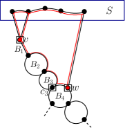
(a) An example of Branching Rule 5.9, with $h=4$. The obstruction is shown in red (light gray), and $v$, $c_{3}$, and $w$ are the three vertices to branch on.

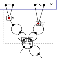
(b) An example of Branching Rule 5.12. Either one vertex among $v,x,y,w$ is in the solution $R$, or all the vertices in the boxed region are not in the solution $R$.

Figure 2: Illustrations of Branching Rules 5.9 and 5.12.

To show that this rule is sound, we need a lemma analogous to Lemma 4 for a “chain of blocks”, which we now define. Let $h\geqslant 3$, and let $B_{1},B_{2},\ldots,B_{h}$ be a set of blocks of $G-S$ that, except for $B_{1}$ and $B_{h}$, contain no red vertices, and for each $i\in\{2,3,\ldots,h-1\}$, the block $B_{i}$ intersects two other blocks in $G-S$: $B_{i-1}$ and $B_{i+1}$. The sequence of blocks $B_{2},B_{3},\ldots,B_{h-1}$ is called a chain of blocks.

Lemma 5

If there is a solution, then there is one that does not contain any vertex of a chain of blocks, except potentially the cut vertex shared by $B_{h-1}$ and $B_{h}$.

Proof

By hypothesis, $B_{h}$ shares one cut vertex $c_{h-1}$ with $B_{h-1}$. From any solution that contains a vertex $v$ in some block in $\{B_{2},B_{3},\ldots,B_{h-1}\}$, one can obtain a new solution by replacing $v$ by $c_{h-1}$.

Recall that $P$ is a chain from $c_{h-1}$ to $w$. The subgraph induced by $V(B_{1})\cup V(B_{2})\cup\cdots\cup V(B_{h-1})\cup P\cup\{w\}\cup V(C)$ contains an obstruction. So, by a combination of Lemmas 4 and 5, we can safely branch on the three vertices $v$, $w$ and $c_{h-1}$. The branching vector is $(1,1,1)$.

Branching Rule 5.10

If $w$ has a neighbor in $S$ in a different connected component than $C$, then branch on putting either $v$, or $w$, or $c_{h-1}$ into the solution $R$, or put $V(B_{1})\cup V(B_{2})\cup\cdots\cup V(B_{h-1})\cup P\cup\{w\}$ in $S$. In each of the first three cases, we remove the vertex from $G$ and decrease $k$ by $1$.

The correctness of this rule is also based on Lemma 5. In the fourth branch, $\text{cc}(S)$ decreases by $1$, so the branching vector is $(1,1,1,1)$.

Once again, we assume that none of the previous rules apply. Let $B^{\prime}$ be a connected component of the block tree $B$ of $G-S$. Assume $B^{\prime}$ has a node that is not a leaf and let us root $B^{\prime}$ at this node. For a vertex $a$ with two neighbors $b$ and $c$, the operation of smoothing $a$ consists of deleting $a$ and adding the edge $bc$. Let $T$ be the rooted tree that we obtain by smoothing each vertex of degree $2$ that is not the root (and keeping the same root). We now consider the parent node $p$ of leaves at the largest depth of $T$. We assume that $p$ is a block $C$. If $p$ is a cut vertex, we get a simplified version of what follows. As $p$ was not smoothed, it has at least two children in $T$, which, by construction, are leaf blocks. We say that two distinct cut vertices $x$ and $y$ are consecutive cut vertices if they are both contained in some block of $G-S$ and there is a chain from $x$ to $y$. We consider two consecutive cut vertices $x$ and $y$ in $C$, and let $B_{x}$ and $B_{y}$ be children of $p$ in $T$ such that $B_{x}\dotsm xC$ and $B_{y}\dotsm yC$ are paths of $B$ for which the internal vertices have degree $2$. Observe that we can find two consecutive cut vertices in $C$, since if one of the vertices of the $xy$-path in $C$ is red, then either Branching Rule 5.9 or Branching Rule 5.10 would apply. Let $v$ (resp. $w$) be the red vertex in $B_{x}$ (resp. $B_{y}$). Recall that $v$ and $w$ have two neighbors in $S$. We branch in the following way:

Branching Rule 5.11

If $v$ and $w$ have their neighbors in $S$ in the same connected component of $G[S]$, then branch on putting either $v$, or $w$, or $x$, or $y$ into the solution $R$. In each case, remove the vertex from $G$ and decrease $k$ by $1$.

Branching Rule 5.12

If $v$ and $w$ have their neighbors in $S$ in distinct connected components of $G[S]$, then branch on putting either $v$, or $w$, or $x$, or $y$ into the solution $R$, or put all of them in $S$ together with the chain from $x$ to $y$ and all the vertices of the blocks in the path from $x$ to $B_{x}$ in $B$ and in the path from $y$ to $B_{y}$ in $B$. In each of the first four cases, remove the vertex from $G$ and decrease $k$ by $1$.

The soundness of these two branching rules is similar to Branching Rules 5.9 and 5.10 and relies on the fact that there is a chain from $x$ to $y$. Their branching vectors are $(1,1,1,1)$ and $(1,1,1,1,1)$ respectively.

Finally, if none of the previous rules apply, the connected components of $G-S$ contain exactly one red vertex. This implies that each of these connected components is a single vertex. Therefore, $G-S$ is an independent set and all the vertices of $V(G)\setminus S$ have exactly two neighbors in $S$. At this point, we could finish the algorithm in polynomial time by observing that the problem is now equivalent to the problem where, given a set of paths in a forest, the task is to find a maximum-sized subset such that the paths are pairwise edge-disjoint. An alternative is to finish with the following simple rule.

Branching Rule 5.13

If $v$ and $w$ are two vertices of $V(G)\setminus S$ such that $G[S\cup\{v,w\}]$ contains an obstruction, then branch on putting either $v$ or $w$ into the solution $R$. In either case, remove the vertex from $G$ and decrease $k$ by $1$.

The soundness of this rule is straightforward and the branching vector is $(1,1)$. When Branching Rule 5.13 cannot be applied, then all the remaining vertices of $V(G)\setminus S$ can safely be put in $S$.

Algorithm 4 Disjoint-BoundedCactusGraphVD($G,S,d,k$)

1:Input: A graph $G$, a subset of vertices $S$, and two integers $d$ and $k$.

2:Output: A set $R$ of size at most $k$ such that $R\cap S=\emptyset$ and $G-R$ is a $d$-cactus graph.

3:Set $R:=\emptyset$.

4:while $k\geqslant 0$ and $G-S$ is non-empty do

5:     if Reduction Rule 5.1, or Branching Rule 5.2, or Reduction Rule 5.7, or Branching Rule 5.5 can be applied then

6:         Apply it

7:     else if Branching Rule 5.6, or Reduction Rule 5.8, or Branching Rule 5.7 can be applied then

8:         Apply it

9:     else if Branching Rule 5.8, or Reduction Rule 5.9, or Reduction Rule 5.10 can be applied then

10:         Apply it

11:     else if Branching Rule 5.9 or Branching Rule 5.10 can be applied then

12:         Apply it

13:     else if Branching Rule 5.11 or Branching Rule 5.12 can be applied then

14:         Apply it

15:     end if

16:end while

17:while Branching Rule 5.13 can be applied do

18:     Apply it

19:end while

20:if $k\geqslant 0$ then

21:     return $R$.

22:end if

The running time of Disjoint Bounded Complete Block VD is given by the worst branching vector $(1,1,1,1,1)$, that is $\mathcal{O}^{*}(5^{\mu(I)})=\mathcal{O}^{*}(25^{k})$.

6 Polynomial Kernels

In this section, we prove the following:

Theorem 6.1

Let $\mathcal{P}$ be a non-degenerate block-hereditary class of graphs recognizable in polynomial time. Then Bounded $\mathcal{P}$-Block Vertex Deletion admits a kernel with $\mathcal{O}(k^{2}d^{7})$ vertices.

Recall that, for positive integers $x$ and $y$, we denote by $\mathcal{B}_{x,y}$ the class of all biconnected graphs with at least $x$ vertices and at most $y$ vertices. We fix a block-hereditary class of graphs $\mathcal{P}$ recognizable in polynomial time. The block tree of a graph can be computed in time $\mathcal{O}(\lvert V(G)\rvert+\lvert E(G)\rvert)$ [10]. Thus, one can test whether a given graph is in $\Phi_{\mathcal{P}\cap\mathcal{B}_{2,d}}$ in polynomial time.

Before describing the algorithm, we observe that there is a $(2d+6)$-approximation algorithm for the (unparameterized) minimization version of the Bounded $\mathcal{P}$-Block Vertex Deletion problem. We first run the algorithm of Proposition 3. When we find an induced subgraph in $(\mathcal{B}_{2,d}\setminus\mathcal{P})\cup\mathcal{B}_{d+1,2d-2}$, instead of branching on the removal of one of the vertices, we remove all the vertices of the subgraph, then rerun the algorithm. Hence, we can reduce to a $(\mathcal{P}\cap\mathcal{B}_{2,d})$-clusterable graph by removing at most $(2d-2)\cdot\operatorname{OPT}$ vertices. Moreover, we can obtain the set of all $(\mathcal{P}\cap\mathcal{B}_{2,d})$-clusters using the algorithm in Lemma 3. Arguments in the proof of Proposition 2 and the known $8$-approximation algorithm for Subset Feedback Vertex Set [8] imply that there is a $(2d+6)$-approximation algorithm for Bounded $\mathcal{P}$-Block Vertex Deletion.

We start with the straightforward reduction rules. Let $(G,d,k)$ be an instance of Bounded $\mathcal{P}$-Block Vertex Deletion.

Reduction Rule 6.1 (Component rule)

If $G$ has a connected component $H\in\Phi_{\mathcal{P}\cap\mathcal{B}_{2,d}}$, then remove $H$.

Reduction Rule 6.2 (Cut vertex rule)

Let $v$ be a cut vertex of $G$ such that $G-v$ contains a connected component $H$ where $G[V(H)\cup\{v\}]$ is a block in $\mathcal{P}\cap\mathcal{B}_{2,d}$. Then remove $H$ from $G$.

Now, we introduce a so-called bypassing rule. We first run the $(2d+6)$-approximation algorithm, and if it outputs a solution of more than $(2d+6)k$ vertices, then we have a No-instance. Thus, we may assume that the algorithm outputs a solution of size at most $(2d+6)k$. Let us fix such a set $U$.

Reduction Rule 6.3 (Bypassing rule)

Let $v_{1},v_{2},\ldots,v_{t}$ be a sequence of cut vertices of $G-U$ with $2\leqslant t\leqslant d+1$, and let $B_{1},\ldots,B_{t-1}$ be blocks of $G-U$ such that

1. for each $i\in\{1,\ldots,t-1\}$, $B_{i}$ is the unique block of $G-U$ containing $v_{i}$ and $v_{i+1}$ and no other cut vertices of $G-U$;

2. $G$ has no edges between $(\bigcup_{1\leqslant i\leqslant t-1}V(B_{i}))\setminus\{v_{1},v_{t}\}$ and $U$; and

3. $\lvert\bigcup_{1\leqslant i\leqslant t-1}V(B_{i}))\rvert\geqslant d+1$.

If $\bigcup_{1\leqslant i\leqslant t-1}V(B_{i})\setminus\{v_{1},\ldots,v_{t}\}=\emptyset$, then contract $v_{1}v_{2}$; otherwise, choose a vertex in $\bigcup_{1\leqslant i\leqslant t-1}V(B_{i})$ that is not a cut vertex of $G-U$, and remove it.

See Fig. 3a for an example application of Reduction Rule 6.3. Note that this rule can be applied in polynomial time using the block tree of $G-U$.

(a)

(b)

Figure 3: An example application of Reduction Rule 6.3 when $d=9$.

$\rightarrow$

Lemma 6

Reduction Rule 6.3 is safe.

Proof

Let $v_{1}v_{2}\cdots v_{t}$ be an induced path of $G-U$ and let $B_{1},\ldots,B_{t-1}$ be blocks of $G-U$ satisfying the conditions of Reduction Rule 6.3. Let $G^{\prime}$ be the resulting graph after applying Reduction Rule 6.3. We show that $G$ has a set of vertices $S$ of size at most $k$ such that $G-S\in\Phi_{\mathcal{P}\cap\mathcal{B}_{2,d}}$ if and only if $G^{\prime}$ has a set of vertices $S^{\prime}$ of size at most $k$ such that $G^{\prime}-S^{\prime}\in\Phi_{\mathcal{P}\cap\mathcal{B}_{2,d}}$. For convenience, let $W:=\bigcup_{1\leqslant i\leqslant t-1}V(B_{i})$.

Suppose that $G$ has a set of vertices $S$ of size at most $k$ such that $G-S\in\Phi_{\mathcal{P}\cap\mathcal{B}_{2,d}}$. If $\lvert S\cap W\rvert\geqslant 1$, then $G-((S\setminus W)\cup\{v_{1}\})$ is also a graph in $\Phi_{\mathcal{P}\cap\mathcal{B}_{2,d}}$, as each block in $\{B_{1},B_{2},\ldots,B_{t-1}\}$ is in $\mathcal{P}\cap\mathcal{B}_{2,d}$. Thus, we may assume that $S\cap W=\emptyset$. Since $\lvert W\rvert\geqslant d+1$, $v_{1}$ and $v_{t}$ are not contained in the same block of $G-S$. It means that there is no path from $v_{1}$ to $v_{t}$ in $G-S$ containing no vertices in $\{v_{2},\ldots,v_{t-1}\}$, and thus all vertices in $\{v_{1},v_{2},\ldots,v_{t}\}$ become cut vertices of $G-S$. Hence, all blocks in $\{B_{1},B_{2},\ldots,B_{t-1}\}$ are in distinct blocks of $G-S$, and thus $G^{\prime}-S$ is in $\Phi_{\mathcal{P}\cap\mathcal{B}_{2,d}}$.

Now suppose that $G^{\prime}$ has a set of vertices $S$ of size at most $k$ such that $G^{\prime}-S\in\Phi_{\mathcal{P}\cap\mathcal{B}_{2,d}}$. When an edge $v_{1}v_{2}$ is contracted, we label the resulting vertex $v_{1}$. Similar to the other direction, if $\lvert S\cap W\rvert\geqslant 1$, then we can replace $S\cap W$ with $v_{1}$. So we may assume that $S\cap W=\emptyset$. As $\lvert V(G^{\prime})\cap W\rvert\geqslant d$ and $G^{\prime}[V(G^{\prime})\cap W]$ is not $2$-connected, $v_{1}$ and $v_{t}$ cannot be contained in the same block of $G^{\prime}-S$. Thus, all blocks of $G^{\prime}$ on $W$ are distinct blocks of $G^{\prime}-S$, so $G-S\in\Phi_{\mathcal{P}\cap\mathcal{B}_{2,d}}$.

We show that after applying Reduction Rules 6.1, 6.2 and 6.3, if the reduced graph is still large, then there is a vertex of large degree. This follows from the fact that the block tree of $G-U$ has no path of $2d+2$ vertices where the internal vertices have degree $2$ in $G-U$.

Lemma 7

Let $(G,d,k)$ be an instance reduced under Reduction Rules 6.1, 6.2 and 6.3. If $(G,d,k)$ is a Yes-instance and $\lvert V(G)\rvert\geqslant 4d(2d+3)(d+3)k\ell$, for some integer $\ell$, then $G$ contains a vertex of degree at least $\ell+1$.

We first require the following lemma.

Lemma 8

Let $T$ be a rooted tree, and let $R\subseteq V(T)$ with $\lvert R\rvert\geqslant 1$. Let $R^{\prime}$ be the set of all nodes in $T$ that are the least common ancestor of two vertices in $R$. Then $\lvert R^{\prime}\rvert\leqslant\lvert R\rvert-1$.

Proof

The proof is by induction on $\lvert R\rvert$. For each node $w$, the subtree rooted at $w$ in $T$ is the subtree of $T$ induced by $w$ and all its descendants. Choose a minimal subtree $T^{\prime}$ rooted at some $z$ containing all nodes in $R$. If $T^{\prime}$ contains precisely one node in $R$, then it contains no nodes in $R^{\prime}$, by definition, and therefore $\lvert R^{\prime}\rvert=0\leqslant\lvert R\rvert-1$. So we may assume that $\lvert R\rvert\geqslant 2$.

Let $z_{1},\ldots,z_{s}$ be the children of $z$ for which the subtree $T_{i}$ rooted at $z_{i}$ contains at least one node in $R$, where $i\in\{1,\ldots,s\}$. Observe that each subtree $T_{i}$ satisfies $|R\cap V(T_{i})|<|R|$, where, in the case that $s=1$, this is because $z\in R$ by the minimality of $T^{\prime}$. Hence, by the induction hypothesis, $\lvert R^{\prime}\cap V(T_{i})\rvert\leqslant\lvert R\cap V(T_{i})\rvert-1$ for each $i\in\{1,\ldots,s\}$. Thus, if $s\geqslant 2$,

$$\lvert R^{\prime}\rvert\leqslant 1+\bigcup_{1\leqslant i\leqslant s}\lvert R^{\prime}\cap V(T_{i})\rvert\leqslant 1+\bigcup_{1\leqslant i\leqslant s}(\lvert R\cap V(T_{i})\rvert-1)\leqslant\lvert R\rvert-1.$$

Otherwise, $s=1$ and $z\in R$, so $|R^{\prime}|\leqslant 1+(\lvert R\cap V(T_{1})\rvert-1)\leqslant\lvert R\rvert-1.$

Proof (Proof of Lemma 7)

Suppose that $\lvert V(G)\rvert\geqslant 4d(2d+3)(d+3)k\ell$ and $G$ has no vertex of degree at least $\ell+1$. Let $T$ be the union of the block trees of connected components of $G-U$. We color some of the nodes of $T$ as follows: for each cut vertex $v$ of $G-U$, color $v$ red if $v$ has a neighbor in $U$; and for each block $B$ of $G-U$, color $B$ red if $B$ contains a vertex that is not a cut vertex in $G-U$ and has a neighbor in $U$. Observe that the number of red nodes in $T$ is at most $2(d+3)k\ell$, since $|U|\leqslant 2(d+3)k$. Arbitrarily pick a root node for each block tree. Now, for every pair of two red vertices, color the least common ancestor in $T$ red. For all nodes that have not been colored red, color them blue. Let $R$ be the set of all red nodes in $T$. Note that $\lvert R\rvert\leqslant 4(d+3)k\ell$ by Lemma 8.

First, we claim that $T$ has no blue nodes of degree at least $3$. Suppose $T$ has a blue node $w$ of degree at least $3$. Then there are at least two connected components of $T-w$ consisting of descendants of $w$ in $T$. If one of the connected components has no red nodes, then this contradicts our assumption that $(G,d,k)$ is reduced under Reduction Rule 6.2. Thus, all the connected components contain red nodes, so $w$ is also colored red, by construction.

Now, we claim that the number of connected components of $T-R$ is at most $4(d+3)k\ell$. We obtain a forest $F$ from $T$ by contracting each maximal monochromatic subgraph $X$ of $T$ into one node with the same color as the nodes of $X$. Note also that all leaf nodes in $F$ are colored red. For each connected component $F^{\prime}$ of $F$, let $R^{\prime}$ be the red nodes in $F^{\prime}$ and let $B^{\prime}$ be the blue nodes in $F^{\prime}$, and arbitrarily choose a root node. Note that there is an injective mapping from $B^{\prime}$ to $R^{\prime}$ that sends a node to one of its children. It follows that the number of blue nodes is at most the number of red nodes in $F$, and thus the number of connected components in $T-R$ is at most $\lvert R\rvert\leqslant 4(d+3)k\ell$.

Note that the number of blocks in $G-U$ is at least $\frac{\lvert V(G-U)\rvert}{d}$, and thus the number of nodes in $T$ is at least $\frac{\lvert V(G-U)\rvert}{d}$. As $\lvert V(G)\rvert\geqslant 4d(2d+3)(d+3)k\ell$, there is a connected component $B$ of $T-R$ where

$$\lvert V(B)\rvert\geqslant\frac{\frac{\lvert V(G-U)\rvert}{d}-\lvert R\rvert}{4(d+3)k\ell}\geqslant\frac{\lvert V(G-U)\rvert-4d(d+3)k\ell}{4d(d+3)k\ell}\geqslant 2d+2.$$

However, this blue connected component with $2d+2$ vertices can be reduced by Reduction Rule 6.3; a contradiction. We conclude that if $(G,d,k)$ is a Yes-instance and $\lvert V(G)\rvert\geqslant 4d(2d+3)(d+3)k\ell$, then $G$ has a vertex of degree at least $\ell+1$.

Now, we discuss a “sunflower structure” that allows us to find a vertex that can be safely removed. A similar technique was used in [1, 13, 21]; there, Gallai’s $A$-path Theorem is used to find many obstructions whose pairwise intersections are exactly one vertex; here, we use different objects to achieve the same thing.

Let $A\subseteq V(G)$ and let $d\geqslant 2$. An $(A,d)$-tree in $G$ is a tree subgraph of $G$ on at least $d$ vertices whose leaves are contained in $A$. Let $v$ be a vertex of $G$. If there is an $(N_{G}(v),d)$-tree $T$ in $G-v$, then $G[V(T)\cup\{v\}]$ is a 2-connected graph with at least $d+1$ vertices. This implies that if there are $k+1$ pairwise vertex-disjoint $(N_{G}(v),d)$-trees in $G-v$, then we can safely remove $v$, as any solution should contain $v$.

We prove that if $G$ does not have any set of $k+1$ pairwise vertex-disjoint $(A,d)$-trees, then there exists $S\subseteq V(G)$ where the size of $S$ is bounded by a function of $k$ and $d$, and every connected component of $G-S$ has fewer than $d$ vertices of $A$. Note that $G-S$ may still have some $(A,d)$-trees, as a path of length $d-1$ between two vertices in $A$ is also an $(A,d)$-tree.

Proposition 4

Let $G$ be a graph, let $k$ and $d$ be positive integers, and let $A\subseteq V(G)$. There is an algorithm that, in time $\mathcal{O}(d\lvert V(G)\rvert^{3})$, finds either:

1. $k$ pairwise vertex-disjoint $(A,d)$-trees in $G$, or

2. a vertex subset $S\subseteq V(G)$ of size at most $2(2k-1)(d^{2}-d+1)$ such that each connected component of $G-S$ contains fewer than $d$ vertices of $A$.

We require the following lemmas.

Lemma 9

Let $k$ and $d$ be positive integers with $d\geqslant 3$. Let $T$ be a tree with maximum degree $d$, and let $A\subseteq V(T)$. If $\lvert A\rvert\geqslant k(d^{2}-d+1)$, then there is an algorithm that finds $k$ pairwise vertex-disjoint $(A,d)$-trees in $T$, in time $\mathcal{O}(k\lvert V(T)\rvert)$.

Proof

If $k=1$, then this is trivial because $d\geqslant 3$. We assume that $k\geqslant 2$. We choose a root node of $T$ that is not a leaf. For each node $t$ in $T$, let $w(t)$ be the number of descendants of $t$ in $A$, where $t$ is considered a descendant of itself. We can compute the value of $w(t)$ for each $t\in T$ in time $\mathcal{O}(\lvert V(T)\rvert)$.

As $\lvert A\rvert\geqslant k(d^{2}-d+1)\geqslant d$, there exists a node $t$ in $T$ with $w(t)\geqslant d$. Choose such a node where $w(t_{1})<d$ for every child $t_{1}$ of $t$. Since $T$ has maximum degree $d$, we have $w(t)\leqslant d(d-1)+1=d^{2}-d+1$. Clearly the subtree rooted at $t$ contains an $(A,d)$-tree. Let $T^{\prime}$ be the connected component of $T-t$ containing the parent of $t$ in $T$. Then $T^{\prime}$ has at least $k(d^{2}-d+1)-(d^{2}-d+1)\geqslant(k-1)(d^{2}-d+1)$ nodes in $A$. Repeating the same procedure on $T^{\prime}$, we can find $k-1$ pairwise vertex-disjoint $(A,d)$-trees in $T^{\prime}$. Thus, we can return $k$ pairwise vertex-disjoint $(A,d)$-trees of $T$ in time $\mathcal{O}(k\lvert V(T)\rvert)$.

Lemma 10

Let $T$ be a tree with no vertices of degree $2$. If $A$ is the set of all leaves of $T$, then $\lvert A\rvert\geqslant\lvert V(T)\setminus A\rvert-2$.

Proof

We note that

• $\lvert A\rvert+\lvert V(T)\setminus A\rvert=\lvert V(T)\rvert=\lvert E(T)\rvert-1$, and

• $\lvert A\rvert+3\lvert V(T)\setminus A\rvert\leqslant\sum_{t\in V(T)}d_{T}(t)=2\lvert E(T)\rvert$.

Combining the two equations, we have that $\lvert A\rvert\geqslant\lvert V(T)\setminus A\rvert-2$, as required.

Proof (Proof of Proposition 4)

We recursively construct a forest $H_{i}$ in $G$ such that each connected component of $H_{i}$ is an $(A,d)$-tree whose maximum degree is at most $d$, until one of the following holds:

1. $H_{i}$ consists of $k$ connected components.

2. $\lvert V(H_{i})\cap A\rvert\geqslant(2k-1)(d^{2}-d+1)$.

3. For the set $S_{i}$ of nodes in $H_{i}$ having degree other than $2$, every connected component of $G-((V(H_{i})\cap A)\cup S_{i})$ has fewer than $d$ vertices of $A$.

In cases (1) and (2), we will return $k$ pairwise vertex-disjoint $(A,d)$-trees, and in case (3), we will return a set $S$ satisfying (ii).

We start with an empty graph $H_{1}$. Let $S_{i}$ be the set of all vertices of degree other than $2$ in $H_{i}$. For the $i$th iteration, choose a connected component $C$ of $G-((V(H_{i})\cap A)\cup S_{i})$ containing at least $d$ vertices of $A$. If there is no such connected component, then we finish the procedure, as (3) holds. So assume that such a connected component $C$ exists. If $V(C)\cap V(H_{i})\neq\emptyset$, then we choose a shortest path $P$ from $A\cap V(C)$ to $V(H_{i})\cap V(C)$, and let $H_{i+1}:=H_{i}\cup P$. As vertices in $A\cap V(C)$ are not contained in $H_{i}$, $\lvert V(H_{i+1})\cap A\rvert\geqslant\lvert V(H_{i})\cap A\rvert+1$. Also, the maximum degree of $H_{i}$ will not change as $P$ will end with a node of degree $2$ in $H_{i}$.

Now, assume that $V(C)\cap V(H_{i})=\emptyset$. In this case, we find an $(A,d)$-tree in $C$ that is disjoint from $H_{i}$. We choose a vertex $s\in V(C)\cap A$, and let $Q_{1}$ be the graph that consists of $s$. For each $j\geqslant 2$, we recursively find a shortest path $P_{i}$ from $V(Q_{j-1})$ to $(V(C)\cap A)\setminus V(Q_{j-1})$ and let $Q_{j}:=Q_{j-1}\cup P_{i}$. It is not hard to see that $Q_{1}$ has maximum degree $0$, and for all $i\in\{2,\ldots,d\}$, $Q_{i}$ has maximum degree $d$. Also, all leaves of $Q_{d}$ are contained in $A$ and $\lvert V(Q_{d})\cap A\rvert=d$. Thus, $Q_{d}$ is an $(A,d)$-tree. We can compute $Q_{d}$ in time $\mathcal{O}(d\lvert V(G)\rvert^{2})$. We set $H_{i+1}:=H_{i}\cup Q_{d}$.

As each iteration strictly increases $V(H_{i})\cap A$, this algorithm will terminate in at most $\lvert V(G)\rvert$ iterations. Let $H$ and $S$ be the final instances $H_{i}$ and $S_{i}$, respectively, prior to termination.

In case (1), each connected component of $H$ contains an $(A,d)$-tree, so we can return $k$ pairwise vertex-disjoint $(A,d)$-trees.

Suppose we have case (2), so $\lvert V(H)\cap A\rvert\geqslant(2k-1)(d^{2}-d+1)$. Let $T_{1},\ldots,T_{h}$ be the connected components of $H$. We may assume that $h\leqslant k-1$. Applying the algorithm of Lemma 9 to $T_{j}$, for each $j\in\{1,\dotsc,h\}$, we can return $\lfloor\frac{\lvert V(T_{j})\cap A\rvert}{d^{2}-d+1}\rfloor$ pairwise vertex-disjoint $(A,d)$-trees in time $\mathcal{O}(\frac{\lvert V(T_{j})\cap A\rvert}{d^{2}-d+1}\lvert V(T_{j})\rvert)$. Therefore, in this case, we can output

$$\sum_{1\leqslant j\leqslant h}\left(\frac{\lvert V(T_{j})\cap A\rvert}{d^{2}-d+1}-1\right)\geqslant\frac{(2k-1)(d^{2}-d+1)-h(d^{2}-d+1)}{d^{2}-d+1}\geqslant k$$

pairwise vertex-disjoint $(A,d)$-trees in time $\mathcal{O}(k\lvert V(G)\rvert)$.

We may now assume that case (3) holds, but case (2) does not, so $\lvert V(H)\cap A\rvert<(2k-1)(d^{2}-d+1)$. By Lemma 10, $\lvert S\rvert\leqslant\lvert V(H)\cap A\rvert+2$, as all leaves of $H$ are contained in $A$. Thus, we have

$$\lvert(V(H)\cap A)\cup S\rvert\leqslant 2\lvert V(H)\cap A\rvert+2\leqslant 2(2k-1)(d^{2}-d+1),$$

and the set $(V(H)\cap A)\cup S$ satisfies (ii).

The total running time of the algorithm is $\mathcal{O}(d\lvert V(G)\rvert^{3})$.

Reduction Rule 6.4 (Sunflower rule 1)

Let $v$ be a vertex of $G$. If there are $k+1$ pairwise vertex-disjoint $(N_{G}(v),d)$-trees in $G-v$, then remove $v$ and reduce $k$ by $1$.

After exhaustively applying Reduction Rule 6.4, we may assume, by Proposition 4, that for each $v\in V(G)$, there exists $S_{v}\subseteq V(G-v)$ with $\lvert S_{v}\rvert\leqslant 2(2k+1)(d^{2}-d+1)$ such that $v$ has at most $d-1$ neighbors in each connected component of $G-(S_{v}\cup\{v\})$. In the remainder of this section, we use $S_{v}$ to denote such a set for any $v\in V(G)$. To find many connected components of $G-(S_{v}\cup\{v\})$ where each connected component $C$ has the property that $G[V(C)\cup\{v\}]\in\phi_{\mathcal{P}\cap\mathcal{B}_{2,d}}$, we apply the next two reduction rules.

Reduction Rule 6.5 (Disjoint obstructions rule)

If there are $k+1$ connected components of $G-(S_{v}\cup\{v\})$ such that each connected component is not in $\phi_{\mathcal{P}\cap\mathcal{B}_{2,d}}$, then conclude that $(G,d,k)$ is a No-instance.

Reduction Rule 6.6 (Sunflower rule 2)

If there are $k+1$ connected components of $G-(S_{v}\cup\{v\})$ where each connected component $C$ is in $\phi_{\mathcal{P}\cap\mathcal{B}_{2,d}}$ but $G[V(C)\cup\{v\}]\notin\phi_{\mathcal{P}\cap\mathcal{B}_{2,d}}$, then remove $v$ and decrease $k$ by $1$.

We can perform these two rules in polynomial time using the block tree of $G[V(C)\cup\{v\}]$. Then we may assume that $G-(S_{v}\cup\{v\})$ contains at most $2k$ connected components such that the connected component $C$ satisfies $G[V(C)\cup\{v\}]\notin\phi_{\mathcal{P}\cap\mathcal{B}_{2,d}}$. Thus, if $v$ has degree at least $\ell$, there are at least $\frac{\ell-2(2k+1)(d^{2}-d+1)}{d-1}-2k$ connected components of $G-(S_{v}\cup\{v\})$ such that the connected component $C$ satisfies $G[V(C)\cup\{v\}]\in\phi_{\mathcal{P}\cap\mathcal{B}_{2,d}}$. As $G$ is reduced under Reduction Rule 6.2, there is an edge between any such connected component $C$ and $S_{v}$. We introduce a final reduction rule, which uses the $\alpha$-expansion lemma [21].

Lemma 11 ($\alpha$-expansion lemma)

Let $\alpha$ be a positive integer, and let $F$ be a bipartite graph with vertex bipartition $(X,Y)$ such that $\lvert Y\rvert\geqslant\alpha\lvert X\rvert$ and every vertex of $Y$ has at least one neighbor in $X$. Then there exist non-empty subsets $X^{\prime}\subseteq X$ and $Y^{\prime}\subseteq Y$ and a function $\phi:X^{\prime}\rightarrow\binom{Y^{\prime}}{\alpha}$ such that

• $N_{F}(Y^{\prime})\cap X=X^{\prime}$,

• $\phi(x)\subseteq N_{F}(x)$ for each $x\in X^{\prime}$, and

• the sets in $\{\phi(x):x\in X^{\prime}\}$ are pairwise disjoint.

In addition, such a pair $X^{\prime},Y^{\prime}$ can be computed in time polynomial in $\alpha\lvert V(F)\rvert$.

Reduction Rule 6.7 (Large degree rule)

Let $v$ be a vertex of $G$. If there is a set $\mathcal{C}$ of connected components of $G-(S_{v}\cup\{v\})$ such that $\lvert\mathcal{C}\rvert\geqslant 2d(2k+1)(d^{2}-d+1)$ and, for each $C\in\mathcal{C}$, we have $G[V(C)\cup\{v\}]\in\phi_{\mathcal{P}\cap\mathcal{B}_{2,d}}$, then do the following:

1. Construct an auxiliary bipartite graph $H$ with bipartition $(S_{v},\mathcal{C})$ where $w\in S_{v}$ and $C\in\mathcal{C}$ are adjacent in $H$ if and only if $w$ has a neighbor in $C$.

2. Compute sets $\mathcal{C}^{\prime}\subseteq\mathcal{C}$ and $S_{v}^{\prime}\subseteq S_{v}$ obtained by applying Lemma 11 to $H$ with $\alpha=d$.

3. Remove all edges in $G$ between $v$ and each connected component $C$ of ${\cal C^{\prime}}$.

4. Add $d-1$ internally vertex-disjoint paths of length $2$ between $v$ and each vertex $x\in S_{v}^{\prime}$.

5. Remove all vertices of degree $1$ in the resulting graph.

Lemma 12

Reduction Rule 6.7 is safe.

Proof

Let $\mathcal{C}$ be a set of connected components of $G-(S_{v}\cup\{v\})$ such that $\lvert\mathcal{C}\rvert\geqslant 2d(2k-1)(d^{2}-d+1)$ and, for $C\in\mathcal{C}$, $G[V(C)\cup\{v\}]\in\phi_{\mathcal{P}\cap\mathcal{B}_{2,d}}$. As $\lvert S_{v}\rvert\leqslant 2(2k-1)(d^{2}-d+1)$, Lemma 11 implies that we can obtain $\mathcal{C}^{\prime}\subseteq\mathcal{C}$, $S_{v}^{\prime}\subseteq S_{v}$ and a function $\phi:S_{v}\rightarrow\binom{\mathcal{C}}{d}$ in polynomial time such that

• $N_{G}(\bigcup_{C\in\mathcal{C}^{\prime}}V(C))\cap S_{v}=S_{v}^{\prime}$,

• $\phi(x)$ is a subset of $\mathcal{C^{\prime}}$ where each connected component in $\phi(x)$ has a neighbor of $x$, and

• the graphs in $\{\bigcup_{C\in\phi(x)}V(C):x\in X\}$ are pairwise disjoint.

Let $G^{\prime}$ be the resulting graph obtained by applying Reduction Rule 6.7. We prove that $(G,d,k)$ is a Yes-instance if and only if $(G^{\prime},d,k)$ is a Yes-instance. Let $R$ be the set of new vertices of degree $2$ between $v$ and $S_{v}^{\prime}$ in $G^{\prime}$.

Suppose that $G^{\prime}$ has a vertex set $A$ with $\lvert A\rvert\leqslant k$ such that $G^{\prime}-A\in\phi_{\mathcal{P}\cap\mathcal{B}_{2,d}}$. If a vertex $r\in R$ is contained in $A$ and $r^{\prime}$ is a neighbor of $r$, then $G^{\prime}-(A\setminus\{r\}\cup\{r^{\prime}\})\in\phi_{\mathcal{P}\cap\mathcal{B}_{2,d}}$, as $r$ and all of its twins become vertices of degree $1$ in $G^{\prime}-(A\setminus\{r\}\cup\{r^{\prime}\})$ and thus they cannot be contained in blocks with at least $3$ vertices. As $d-1$ distinct paths of length $2$ from $v$ to a vertex $x\in S_{v}^{\prime}$ form a block with $d+1$ vertices, we may assume that $A$ contains either $v$ or $x$. Considering all vertices in $S_{v}^{\prime}$, we have either $v\in A$ or $S_{v}^{\prime}\subseteq A$. If $v\in A$, then $G-A$ is an induced subgraph of $G^{\prime}-A$, and therefore, $G-A\in\phi_{\mathcal{P}\cap\mathcal{B}_{2,d}}$. Suppose $v\notin A$ and $S_{v}^{\prime}\subseteq A$. Since $N_{G}(\bigcup_{C\in\mathcal{C}^{\prime}}V(C))\cap S_{v}=S_{v}^{\prime}$, $v$ is a cut vertex of $G-A$, and we know that $G[V(C)\cup\{v\}]\in\phi_{\mathcal{P}\cap\mathcal{B}_{2,d}}$ for all $C\in\mathcal{C}^{\prime}$. Moreover, $G-A-(\bigcup_{C\in\mathcal{C}}V(C))$ is an induced subgraph of $G^{\prime}-A$, and thus it is a graph in $\phi_{\mathcal{P}\cap\mathcal{B}_{2,d}}$. Therefore, $G-A\in\phi_{\mathcal{P}\cap\mathcal{B}_{2,d}}$.

For the converse direction, suppose that $G$ has a vertex set $A$ with $\lvert A\rvert\leqslant k$ such that $G-A\in\phi_{\mathcal{P}\cap\mathcal{B}_{2,d}}$. If $v\in A$, then the vertices in $R$ become pendant vertices in $G^{\prime}-A$, and thus, $G^{\prime}-A\in\phi_{\mathcal{P}\cap\mathcal{B}_{2,d}}$. We may assume that $v\notin A$.

Let $A_{1}:=S_{v}^{\prime}\setminus A$ and $A_{2}:=A\cap(\bigcup_{C\in\mathcal{C}^{\prime}}V(C))$. It is not hard to see that $G-((A\setminus A_{2})\cup A_{1})\in\phi_{\mathcal{P}\cap\mathcal{B}_{2,d}}$ as $G[V(C)\cup\{v\}]\in\phi_{\mathcal{P}\cap\mathcal{B}_{2,d}}$ for each $C\in\mathcal{C}^{\prime}$. We claim that $\lvert A_{2}\rvert\geqslant\lvert A_{1}\rvert$, which implies that there is a vertex set $A^{\prime}$ with $\lvert A^{\prime}\rvert\leqslant\lvert A\rvert\leqslant k$ such that $G^{\prime}-A^{\prime}\in\phi_{\mathcal{P}\cap\mathcal{B}_{2,d}}$. Suppose $\lvert A_{2}\rvert<\lvert A_{1}\rvert$. Since the sets in $\{\bigcup_{C\in\phi(x)}V(C):x\in S_{v}^{\prime}\}$ are pairwise disjoint, there exists a vertex $a$ in $A_{1}$ such that $\phi(a)$ contains no vertex from $A_{2}$. Then $d-1$ connected components in $\phi(a)$ with the vertices $v$ and $a$ contains a $2$-connected subgraph with at least $d+1$ vertices, which contradicts the assumption that $G-A\in\phi_{\mathcal{P}\cap\mathcal{B}_{2,d}}$.

Lemma 13

Reduction Rules 6.1, 6.2, 6.3, 6.4, 6.5, 6.6 and 6.7 can be applied exhaustively in polynomial time.

Proof

It is clear that an application of one of Reduction Rules 6.1, 6.2, 6.3, 6.4, 6.5 and 6.6 decreases $\lvert V(G)\rvert$. We show that $\lvert V(G)\rvert+\lvert E^{\prime}\rvert$ decreases when Reduction Rule 6.7 is applied, where $E^{\prime}$ is the number of edges of $G$ for which both end vertices have degree at least $3$.

Let $(G,d,k)$ be an instance, and let $E^{\prime}$ be the set of edges where both end vertices have degree at least $3$. First, observe that $\lvert V(G)\rvert+\lvert E^{\prime}\rvert$ is increased by $(d-1)\lvert S_{v}^{\prime}\rvert$ when adding $d-1$ disjoint paths of length $2$ from $v$ to each vertex of $S_{v}^{\prime}$. It is sufficient to check that for each $C\in\mathcal{C}^{\prime}$, $\lvert V(G)\rvert+\lvert E^{\prime}\rvert$ is decreased by at least $1$, since $\lvert\mathcal{C}^{\prime}\rvert\geqslant d\lvert S_{v}^{\prime}\rvert>(d-1)\lvert S_{v}^{\prime}\rvert$. If $v$ has a neighbor in $C\in\mathcal{C}^{\prime}$ that has degree $3$ in $G$, then this is clear. If a neighbor $w$ of $v$ in $C\in\mathcal{C}^{\prime}$ has degree $2$ in $G$, then it becomes a vertex of degree $1$ and will be removed when applying Reduction Rule 6.7. Since every neighbor of $v$ in a connected component of $\mathcal{C}^{\prime}$ has degree at least $2$, this completes the proof.

Proof (Proof of Theorem 6.1)

We apply Reduction Rules 6.1, 6.2, 6.3, 6.4, 6.5, 6.6 and 6.7 exhaustively. Note that this takes polynomial time, by Lemma 13. Suppose that $(G,d,k)$ is the reduced instance, and $\lvert V(G)\rvert\geqslant 4dk(\ell-1)(2d+3)(d+3)$ where $\ell=2d^{2}(2k+1)(d^{2}-d+3)$. Then, by Lemma 7, there exists a vertex $v$ of degree at least $\ell$.

By Proposition 4, $v$ has at most $d-1$ neighbors in each connected component of $G-(S_{v}\cup\{v\})$. Since $\ell=2d^{2}(2k+1)(d^{2}-d+3)$, the subgraph $G-(S_{v}\cup\{v\})$ contains at least $\frac{\ell-2(2k+1)(d^{2}-d+1)}{d-1}\geqslant 2d(2k+1)(d^{2}-d+3)$ connected components. By Reduction Rules 6.5 and 6.6, $G-(S_{v}\cup\{v\})$ contains at least $2d(2k+1)(d^{2}-d+1)$ connected components such that, for each connected component $C$, $G[V(C)\cup\{v\}]\in\phi_{\mathcal{P}\cap\mathcal{B}_{2,d}}$. Then we can apply Reduction Rule 6.7, contradicting our assumption. We conclude that $\lvert V(G)\rvert=\mathcal{O}(k^{2}d^{7})$.

One might ask whether the kernel with $\mathcal{O}(k^{2}d^{7})$ vertices can be improved upon. Regarding the $k^{2}$ factor, reducing it to linear in $k$ would imply a linear kernel for Feedback Vertex Set. On the other hand, it is possible to reduce the $d^{7}$ factor depending on the block-hereditary class $\mathcal{P}$.

Theorem 6.2

• Bounded Block VD admits a kernel with $\mathcal{O}(k^{2}d^{6})$ vertices.

• Bounded Complete Block VD admits a kernel with $\mathcal{O}(k^{2}d^{3})$ vertices.

• Bounded Cactus Graph VD admits a kernel with $\mathcal{O}(k^{2}d^{4})$ vertices.

We prove Theorem 6.2 as three separate results: Theorems 6.3, 6.4 and 6.5.

First, observe that each of the three problems have $(2d+6)$-approximation algorithms, by the same argument as for the general problem Bounded $\mathcal{P}$-Block Vertex Deletion.

Now consider the Bounded Block VD problem. All the reduction rules for Bounded $\mathcal{P}$-Block Vertex Deletion can be applied with $\mathcal{P}$ as the class of all biconnected graphs. However, Reduction Rule 6.3 can be modified as follows, in order to obtain a slightly better kernel. Let $(G,d,k)$ be an instance of Bounded Block VD, and let $U$ be a solution of size at most $(2d+6)k$ obtained by the $(2d+6)$-approximation algorithm.

Reduction Rule 6.8 (Bypassing rule 2)

Let $v_{1},v_{2},v_{3}$ be a sequence of cut vertices of $G-U$, and let $B_{1}$ and $B_{2}$ be blocks of $G-U$ such that

1. for each $i\in\{1,2\}$, $B_{i}$ is the unique block containing $v_{i}$, $v_{i+1}$ and no other cut vertices, and

2. $G$ has no edges between $(V(B_{1})\cup V(B_{2}))\setminus\{v_{1},v_{3}\}$ and $U$.

Then remove $(V(B_{1})\cup V(B_{2}))\setminus\{v_{1},v_{3}\}$ and add a clique of size $\min\{d,\lvert V(B_{1})\cup V(B_{2})\rvert\}$ containing $v_{1}$ and $v_{3}$.

Lemma 14

Reduction Rule 6.8 is safe.

Proof

Let $v_{1}v_{2}v_{3}$ be an induced path of $G-U$ and let $B_{1}$ and $B_{2}$ be blocks of $G-U$ satisfying the conditions of Reduction Rule 6.8. Let $G^{\prime}$ be the resulting graph after applying Reduction Rule 6.8. We show that $G$ has a set of vertices $S$ of size at most $k$ such that $G-S\in\Phi_{\mathcal{B}_{2,d}}$ if and only if $G^{\prime}$ has a set of vertices $S^{\prime}$ of size at most $k$ such that $G^{\prime}-S^{\prime}\in\Phi_{\mathcal{B}_{2,d}}$. For convenience, let $W:=V(B_{1})\cup V(B_{2})$, and let $W^{\prime}$ be the new clique added in $G^{\prime}$.

Suppose that $G$ has a set of vertices $S$ of size at most $k$ such that $G-S\in\Phi_{\mathcal{B}_{2,d}}$. If $\lvert S\cap W\rvert\geqslant 1$, then $G-((S\setminus W)\cup\{v_{1}\})$ is a graph in $\Phi_{\mathcal{B}_{2,d}}$, as $B_{1}$ and $B_{2}$ are in $\mathcal{B}_{2,d}$. Thus, $G^{\prime}-((S\setminus W)\cup\{v_{1}\})$ is also a graph in $\Phi_{\mathcal{B}_{2,d}}$. We may now assume that $S\cap W=\emptyset$. Assume that $W$ is contained in some block $B$ of $G-S$. In this case, $\lvert W\rvert\leqslant d-1$ as $G[W]$ is not $2$-connected. Thus, $G^{\prime}-S\in\Phi_{\mathcal{B}_{2,d}}$, as the block obtained from $B$ by replacing $W$ with $W^{\prime}$ has the same number of vertices, and all the other blocks are the same. If $W$ is not contained in some block of $G-S$, then every path from $v_{1}$ to $v_{3}$ in $G-S$ passes through $v_{2}$. Thus, $v_{1}$, $v_{2}$, and $v_{3}$ are cut vertices of $G-S$. Hence, $B_{1}$ and $B_{2}$ are distinct blocks of $G-S$, and thus $G^{\prime}-S$ is in $\Phi_{\mathcal{B}_{2,d}}$.

Now suppose that $G^{\prime}$ has a set of vertices $S$ of size at most $k$ such that $G^{\prime}-S\in\Phi_{\mathcal{B}_{2,d}}$. Similar to the other direction, if $\lvert S\cap W\rvert\geqslant 1$, then we can replace $S\cap W$ with $v_{1}$. So we may assume that $S\cap W=\emptyset$. If $W^{\prime}$ is a block of $G^{\prime}-S$, then $v_{1}$ and $v_{3}$ are cut vertices of $G^{\prime}-S$, and one can easily check that $G-S\in\Phi_{\mathcal{B}_{2,d}}$. Otherwise, the clique $W^{\prime}$ is not a block of $G^{\prime}-S$, that is, it is contained in a bigger block. Then $\lvert W^{\prime}\rvert\leqslant d-1$ and $\lvert W\rvert=\lvert W^{\prime}\rvert\leqslant d-1$, and thus $G-S$ is also in $\Phi_{\mathcal{B}_{2,d}}$.

Theorem 6.3

Bounded Block VD admits a kernel with $\mathcal{O}(k^{2}d^{6})$ vertices.

Proof

Lemma 14 implies that the block tree of $G-U$ has no path of $6$ vertices whose internal vertices have degree $2$ in $G-U$. By modifying Lemma 7, we can show that if $(G,d,k)$ is reduced under Reduction Rules 6.1, 6.2 and 6.8, and $\lvert V(G)\rvert\geqslant 28d(d+3)k\ell$, then $G$ has a vertex of degree at least $\ell+1$. Using Reduction Rules 6.4, 6.5, 6.6 and 6.7 and the same argument as in the proof of Theorem 6.1, it follows that there is a kernel with $\mathcal{O}(k^{2}d^{6})$ vertices.

Note that we can also use Reduction Rule 6.8 for Bounded Complete Block VD, since for complete-block graphs, every maximal clique cannot be contained in a bigger block. But it seems difficult to obtain a similar rule for Bounded Cactus Graph VD. However, for both problems, we can obtain a smaller kernel by using different objects in Proposition 4.

Recall that a graph $G$ is a $d$-complete block graph if every block of $G$ is a complete graph with at most $d$ vertices, and a graph $G$ is a $d$-cactus if it is a cactus graph and every block has at most $d$ vertices.

Theorem 6.4

Bounded Cactus Graph VD admits a kernel with $\mathcal{O}(k^{2}d^{4})$ vertices.

Proof

We observe that for a vertex $v$ in a graph $G$ and an $(N_{G}(v),3)$-tree $T$, $G[V(T)\cup\{v\}]$ is $2$-connected and it is not a cycle. Thus $G[V(T)\cup\{v\}]$ is not a $d$-cactus graph, and at least one vertex of $V(T)\cup\{v\}$ should be taken in any solution. Because of this, we can replace $(N_{G}(v),d)$-trees with $(N_{G}(v),3)$-trees in Reduction Rule 6.4. By Proposition 4, we may assume that for each $v\in V(G)$, there exists $S_{v}\subseteq V(G-v)$ with $\lvert S_{v}\rvert\leqslant 14(2k+1)$ such that $v$ has at most $2$ neighbors in each connected component of $G-(S_{v}\cup\{v\})$.

Note that if there are two vertices with three vertex-disjoint paths between them, then we have a subdivision of the diamond, which is an obstruction for cactus graphs. Thus, the number of connected components of $G-(S_{v}\cup\{v\})$ required for Reduction Rule 6.7 to be applicable can be changed to $(3+1)\cdot 14(2k+1)=56(2k+1)$.

We set $\ell:=112(2k+3)$. Suppose that $(G,d,k)$ is the reduced instance, and $\lvert V(G)\rvert\geqslant 4dk(\ell-1)(2d+3)(d+3)$. Then, by Lemma 7, there exists a vertex $v$ of degree at least $\ell$.

Since $\ell=112(2k+3)$, $G-(S_{v}\cup\{v\})$ contains at least $\frac{\ell-14(2k+1)}{2}\geqslant 56(2k+3)$ connected components. By Reduction Rules 6.5 and 6.6, $G-(S_{v}\cup\{v\})$ contains at least $56(2k+1)$ connected components such that, for each connected component $C$, $G[V(C)\cup\{v\}]$ is a $d$-cactus. Then we can apply Reduction Rule 6.7, contradicting our assumption. We conclude that $\lvert V(G)\rvert=\mathcal{O}(k^{2}d^{3})$.

For Bounded Complete Block VD we can use Gallai’s $A$-path Theorem instead of Proposition 4. The following can be obtained by modifying [13, Proposition 3.1] so that the size of blocks is also taken into account.

Proposition 5 ([13])

Let $G$ be a graph and let $v\in V(G)$ and let $k$ be a positive integer. Then, in $\mathcal{O}(kn^{3})$ time, we can find either

1. $k+1$ obstructions for $d$-complete block graphs that are pairwise vertex-disjoint, or

2. $k+1$ obstructions for $d$-complete block graphs whose pairwise intersections are exactly the vertex $v$, or

3. $S_{v}\subseteq V(G)$ with $\lvert S_{v}\rvert\leqslant 7k$ such that $G-S_{v}$ has no obstruction for $d$-complete block graphs containing $v$.

Theorem 6.5

Bounded Complete Block VD admits a kernel with $\mathcal{O}(k^{2}d^{3})$ vertices.

Proof

We exhaustively reduce using Reduction Rules 6.1, 6.2, 6.8, 6.4, 6.5, 6.6 and 6.7. Now, applying Proposition 5, we can assume that for each $v\in V(G)$, there exists $S_{v}\subseteq V(G-v)$ with $\lvert S_{v}\rvert\leqslant 7k$ such that $G-S_{v}$ has no obstruction for $d$-complete block graphs containing $v$. But we cannot say anything about the number of neighbors of $v$ in each connected component of $G-S_{v}$ after reducing in case (i) or case (ii). So we find a $(2d+6)$-approximation solution $U$ and let $U^{*}:=U$ if $v\notin U$ and $U^{*}:=U\setminus\{v\}$ otherwise, and add it to $S_{v}$. Then $G-(S_{v}\cup U^{*})$ is a $d$-complete block graph and $v$ has at most $d-1$ neighbors in each connected component of $G-(S_{v}\cup U^{*})$.

Note that if there are two vertices with two vertex-disjoint paths of length at least $2$ between them, then there is an obstruction for $d$-complete block graphs. So we can use the $3$-expansion lemma as in [13]. Thus, the number of connected components required for Reduction Rule 6.7 to be applicable can be changed to $3(7k+(2d+6)k)=3k(2d+13)$.

We set $\ell:=3kd(2d+13)$. Suppose that $(G,d,k)$ is the reduced instance, and $\lvert V(G)\rvert\geqslant 28d(d+3)k\ell$. By modifying Lemma 7, one can show that $G$ has a vertex of degree at least $\ell+1$.

Since $\ell=3kd(2d+13)$, $G-(S_{v}\cup U^{*}\cup\{v\})$ contains at least $\frac{\ell-k(2d+13)}{(d-1)}\geqslant 3k(2d+13)$ connected components. So we can reduce the instance using the $3$-expansion lemma; a contradiction. We conclude that $\lvert V(G)\rvert=\mathcal{O}(k^{2}d^{4})$.

References

- [1] Agrawal, A., Kolay, S., Lokshtanov, D.: A faster FPT algorithm and a smaller kernel for Block Graph Vertex Deletion. In: Proceedings of the 12th Latin American Theoretical Informatics Symposium (LATIN 2016). Lecture Notes in Computer Science, Springer (2016)
- [2] Bondy, J.A., Murty, U.S.R.: Graph theory, Graduate Texts in Mathematics, vol. 244. Springer, New York (2008)
- [3] Cai, L.: Fixed-parameter tractability of graph modification problems for hereditary properties. Information Processing Letters 58(4), 171–176 (1996)
- [4] Cygan, M., Fomin, F.V., Kowalik, L., Lokshtanov, D., Marx, D., Pilipczuk, M., Pilipczuk, M., Saurabh, S.: Parameterized Algorithms. Springer (2015)
- [5] Downey, R.G., Fellows, M.R.: Fundamentals of Parameterized Complexity. Texts in Computer Science, Springer (2013)
- [6] Drange, P.G., Dregi, M.S., van ’t Hof, P.: On the computational complexity of vertex integrity and component order connectivity. In: Algorithms and Computation: 25th International Symposium, ISAAC 2014, Jeonju, Korea, December 15–17, 2014, Proceedings. pp. 285–297 (2014)
- [7] El-Mallah, E.S., Colbourn, C.J.: The complexity of some edge deletion problems. IEEE Trans. Circuits and Systems 35(3), 354–362 (1988)
- [8] Even, G., Naor, J., Zosin, L.: An -approximation algorithm for the subset feedback vertex set problem. SIAM J. Comput. 30(4), 1231–1252 (2000)
- [9] Fomin, F., Lokshtanov, D., Misra, N., Saurabh, S.: Planar -Deletion: Approximation and Optimal FPT Algorithms. In: Foundations of Computer Science (FOCS). pp. 470–479 (2012)
- [10] Hopcroft, J., Tarjan, R.: Algorithm 447: Efficient algorithms for graph manipulation. Commun. ACM 16(6), 372–378 (1973)
- [11] Impagliazzo, R., Paturi, R., Zane, F.: Which problems have strongly exponential complexity? J. Comput. System Sci. 63(4), 512–530 (2001)
- [12] Joret, G., Paul, C., Sau, I., Saurabh, S., Thomassé, S.: Hitting and Harvesting Pumpkins. SIAM J. Discrete Math. 28(3), 1363–1390 (2014)
- [13] Kim, E.J., Kwon, O.: A Polynomial Kernel for Block Graph Deletion. In: Husfeldt, T., Kanj, I. (eds.) 10th International Symposium on Parameterized and Exact Computation (IPEC 2015). Leibniz International Proceedings in Informatics (LIPIcs), vol. 43, pp. 270–281. Schloss Dagstuhl–Leibniz-Zentrum fuer Informatik, Dagstuhl, Germany (2015)
- [14] Kim, E.J., Langer, A., Paul, C., Reidl, F., Rossmanith, P., Sau, I., Sikdar, S.: Linear kernels and single-exponential algorithms via protrusion decompositions. In: Automata, Languages, and Programming - 40th International Colloquium, ICALP 2013, Riga, Latvia, July 8-12, 2013, Proceedings, Part I. pp. 613–624 (2013)
- [15] Kolay, S., Lokshtanov, D., Panolan, F., Saurabh, S.: Quick but Odd Growth of Cacti. In: Husfeldt, T., Kanj, I. (eds.) 10th International Symposium on Parameterized and Exact Computation (IPEC 2015). pp. 258–269. No. 43, Schloss Dagstuhl–Leibniz-Zentrum fuer Informatik, Dagstuhl, Germany (2015)
- [16] Lewis, J.M., Yannakakis, M.: The node-deletion problem for hereditary properties is NP-complete. J. Comput. Syst. Sci. 20(2), 219–230 (1980)
- [17] Lokshtanov, D., Marx, D., Saurabh, S.: Slightly superexponential parameterized problems. In: Proceedings of the Twenty-Second Annual ACM-SIAM Symposium on Discrete Algorithms, SODA 2011, San Francisco, California, USA, January 23-25, 2011. pp. 760–776 (2011)
- [18] Misra, P., Raman, V., Ramanujan, M.S., Saurabh, S.: Graph-Theoretic Concepts in Computer Science: 38th International Workshop, WG 2012, Jerusalem, Israel, June 26-28, 2012, Revised Selected Papers, chap. Parameterized Algorithms for Even Cycle Transversal, pp. 172–183. Springer Berlin Heidelberg, Berlin, Heidelberg (2012)
- [19] Reed, B.A., Smith, K., Vetta, A.: Finding odd cycle transversals. Oper. Res. Lett. 32(4), 299–301 (2004)
- [20] Robertson, N., Seymour, P.D.: Graph Minors. XIII. The Disjoint Paths Problem. J. Comb. Theory B 63, 65–110 (1995)
- [21] Thomassé, S.: A quadratic kernel for feedback vertex set. In: Proceedings of the Twentieth Annual ACM-SIAM Symposium on Discrete Algorithms, SODA 2009, New York, NY, USA, January 4-6, 2009. pp. 115–119 (2009)
- [22] Wahlström, M.: Half-integrality, LP-branching and FPT algorithms. In: Proceedings of the Twenty-Fifth Annual ACM-SIAM Symposium on Discrete Algorithms. pp. 1762–1781. SIAM (2014)