Entanglement Entropy of the ${\mathcal{N}}=4$ SYM spin chain

Abstract

We present a detailed study of the Entanglement Entropy (EE) of excited states in all closed rank one subsectors of ${\cal N}=4$ SYM, namely $SU(2)$, $SU(1|1)$ and $SL(2)$. Exploiting the techniques of the Coordinate and the Algebraic Bethe Ansatz we obtain the EE for spin chains with up to seven magnons, at leading order in the coupling expansion but exact in the length of the spin chain and of the part of it that we cut. Focusing on the superconformal primary operator with two magnons in the BMN limit, we derive analytic and exact, in the coupling $\lambda^{\prime}$, expressions for the Renyi and the EE. The interpolating functions for the Renyi and the EE monotonically increase as the coupling increases from the weak coupling $\lambda^{\prime}\rightarrow 0$ regime to the strong coupling $\lambda^{\prime}\rightarrow\infty$ regime. This results to a violation of a certain bound for the EE that is present at weak coupling and confirms the physical intuition that entanglement increases when the coupling increases.

1 Introduction

One of the most intriguing features of a quantum system is that of entanglement. When a physical system is in an entangled state local measurements at one point may instantaneously affect the result of local measurements at distant points. A universal measure of entanglement is the Entanglement Entropy (EE). It can be defined for any quantum field theory or many-body system and unlike correlation functions is a non-local quantity. Suppose we are given a quantum system, e.g. a quantum field theory in $d+1$ dimensions. Furthermore, suppose that we split the system in two parts, $D$ and its complementary $D^{C}$. Assuming that the full Hilbert space of the theory $H$ can be written as the direct product of the Hilbert spaces of the parts $D$ and $D^{C}$, namely $H=H_{D}\otimes H_{D^{C}}$, one can define the reduced density matrix (RDM) of region $D$ in the following way

$$\rho_{D}\,=\,Tr_{D^{C}}\rho\,,\quad\rm{where}\quad\rho=|\psi\rangle\langle\psi|\,,$$ (1.1)

if the system is in a pure quantum state $|\psi\rangle$. Then the EE is defined as the von Neumann entropy of the reduced density matrix, which as can be seen from (1.1) is obtained when we trace out the degrees of freedom of the complementary region $D^{C}$

$$S_{EE}(D)\,=\,-\,\text{Tr}\big{[}\rho_{D}\,\log{\rho_{D}}\big{]}\,.$$ (1.2)

Physically, the EE indicates to what extend the two subsystems, $D$ and $D^{C}$, are correlated. Equivalently, one can also interpret the EE as the entropy measured by an observer sitting in the region $D$ who has no access to information about the subsystem $D^{C}$.

Furthermore, since the EE is defined as the von Neumann entropy one should expect that it is, somehow, related to the degrees of freedom of the system under consideration. This expectation is fully realised in the context of two dimensional conformal field theories ($2d$ CFTs) where the universal piece of the EE is proportional to the central charge Holzhey:1994we ; Calabrese:2004eu . Indeed, for a one-dimensional system with periodic boundary conditions at the critical point, the EE for an interval of length $l$ is given by

$$S_{EE}(l)\,=\,\frac{c}{3}\,\log{\left(\frac{L}{\pi a}\,\sin{\frac{\pi l}{L}}\right)}\quad\text{with}\quad S_{EE}(l)\,\approx\,\frac{c}{3}\,\log{\frac{l}{a}}\quad\rm{for}\quad L\rightarrow\infty$$ (1.3)

where $c$ is the central charge of the corresponding CFT, $a$ is a UV cut–off and $L$ is the length of the whole system. Based on the holographic proposal of Ryu & Takayanagi (RT) Ryu:2006bv ; Ryu:2006ef for the EE of a higher dimensional quantum field theory, it seems that the proportionality between the EE and the central charge of a CFT in four dimensions also holds. The holographic proposal for calculating the EE has been proved for spherical entangling regions Casini:2011kv and there are supporting arguments based on the notion of generalised entropy Lewkowycz:2013nqa .

As opposed to the thermal entropy, the EE is non-vanishing at zero temperature. Therefore, we can employ it to probe the quantum properties of the ground state for a given quantum system. Additionally it can be used as an order parameter for the study of quantum phase transitions at zero temperature Klebanov:2007ws ; Georgiou:2015pia .

The vast majority of the results obtained so far in the literature have been devoted to the entanglement properties of the vacuum state. Comparatively, very little is known about the behaviour of the EE when the system under consideration is in an excited state (see for example Alba:2009th ). The aim of this work is to contribute towards this direction. In particular, we will focus our attention at one of the mostly studied conformal field theories, namely the maximally supersymmetric field theory in four dimensions c. It is well-known that the operators of ${\cal N}=4$ SYM can be mapped to states of an integrable spin-chain, while the dilatation operator can be mapped to a long-range spin-chain Hamiltonian whose eigenvalues give the spectrum of the dilatation operator Beisert:2010jr . Furthermore, through the AdS/CFT correspondence Maldacena:1997re (for a set of pedagogical introductions see Ramallo:2013bua ; Edelstein:2009iv ) the gauge theory operators are dual to certain string states propagating on the $AdS_{5}\times S^{5}$ background with the energies of the string states being equal to the dimension of the dual field theory operator.

We should mention that the Entanglement Entropy that we are about to calculate is not directly related to the EE of ${\cal N}=4$ SYM as a field theory. Such entropy measures the entanglement of a 3-dimensional subregion of the manifold on which the theory is defined to the rest of the space. What we will calculate is the EE of a portion of the ${\cal N}=4$ SYM spin chain, when the chain is in an excited state of either one of the closed rank one subsectors of ${\cal N}=4$ SYM or in the full $PSU(2,2|4)$ algebra of ${\cal N}=4$ SYM, in the case of the BMN limit. The important point is that, through the AdS/CFT correspondence, the EE of the spin chain should be somehow related to the EE of the corresponding string state, that is to the EE of an excited state of the $1+1-$dimensional supersymmetric non-linear $\sigma-$ model which describes the propagation of the corresponding string in the AdS background. As it is extremely complicated to calculate this quantity directly from the $\sigma-$ model considered as a field theory, our intension is to see if one can extract some information from the corresponding spin chain picture where the calculation is considerably easier.

The plan of the paper is as follows: In Section 2 we will analytically calculate the EE of excited states with two magnons in all closed rank one subsectors of ${\cal N}=4$ SYM, namely $SU(2)$, $SU(1|1)$ and $SL(2)$. Our calculation will be performed using the formalism of Coordinate Bethe Ansatz (CBA) and will be leading in the coupling expansion (our states will be the eigenstates of the one-loop dilatation operators) but exact in the length of the spin chain and of the part of it we cut, namely $D$.

In Section 3 we will calculate the EE of the superconformal primary operator with two excitations in the BMN limit. We will derive an analytic expression for the EE of which is exact in the coupling $\lambda^{\prime}=\frac{g_{YM}^{2}N}{J^{2}}=\frac{\lambda}{J^{2}}$. This will allows us to analyse the effect of long-range interactions of the spin chain on the EE. In particular, we will see that the EE of a part of the spin chain is a monotonically increasing function of the coupling which saturates to a constant value as $\lambda^{\prime}\rightarrow\infty$ when keeping the length of the chain we cut fixed. This results to a violation of a certain bound for the EE that is present at weak coupling. Thus, one of our main conclusions is that, as it is physically anticipated, the entanglement between parts of the chain becomes stronger as one increases the coupling $\lambda^{\prime}$, at least for the superconformal primary operator with two excitations.

In Section 4 we will employ integrability and more precisely the powerful formalism of the Algebraic Bethe Ansatz (ABA) in order to calculate numerically the EE of excited states with up to seven magnons in the $SU(2)$, $SU(1|1)$ and $SL(2)$ subsectors. Finally, in Section 5 we will present our conclusions along with directions for future research.

2 Entanglement entropy of two magnons in the three rank one closed subsectors of the ${\cal N}=4$ spin chain

As discussed in the introduction, it is of the outmost importance to calculate the EE for the excited states of any physical system. This task is extremely difficult but it could provide highly non-trivial information about the physical system under consideration. For example, the EE can be viewed as the order parameter characterising the phase transitions which the system might undergo, (see e.g. Georgiou:2015pia ).

In this section, and having the AdS/CFT correspondence in mind, we will focus on the case of two magnons propagating in the ${\mathcal{N}}=4$ SYM spin chain. In particular we will consider operators in each of the three rank one closed subsectors of ${\mathcal{N}}=4$ SYM, namely $SU(2)$, $SU(1|1)$ and $SL(2)$. We will derive analytic expressions for any two magnon state in all the aforementioned sectors by employing the CBA.

As is well known, the problem of finding the eigenvalues and the eigenvectors of the dilatation operator of ${\mathcal{N}}=4$ SYM can be solved by mapping this operator to the Hamiltonian of a certain integrable long-range spin chain. Then one can apply the method of Perturbative Asymptotic Bethe Ansatz (see Staudacher:2004tk for details about this method) to solve for the eigenstates and the eigenvalues. If one is restricted to the one loop case, then the powerful technique of the ABA can be employed. It is this method that we will use in the following to obtain the EE for spin chains with different lengths and up to seven magnons.

2.1 Entanglement Entropy of the vacuum

We will take the operator corresponding to the vacuum state to be

$${\cal O}_{vac}\,\sim\,\text{Tr}\big{[}Z^{L}\big{]}\,.$$ (2.4)

This is a BPS operator whose engineering dimension is $L$. This dimension is not altered by quantum corrections. The corresponding spin chain state is given by

$$|\downarrow\rangle_{vac}\,=\,\,\prod_{i=1}^{L}\,\otimes\,|\downarrow\rangle_{i}\,.$$ (2.5)

When the system is in the ground state (2.5) the EE of any part of the spin chain $D$ is zero, i.e. $S_{EE}(D)=0$, since (2.5) can be written as a direct product of states at each site.

2.2 Entanglement Entropy of a state with one magnon

It is straightforward to consider the case where the wavefunction of the system is that of a giant magnon with momentum $p$. Although this is not a legitimate state since the cyclicity of the trace will necessarily set $p=0$, one can consider this state as a building block of states with more than one excitations. In a spin chain language the eigenstate of a giant magnon is given by

$$|\psi\rangle_{magnon}\,\sim\,\sum_{l=0}^{L}e^{ipl}\,|\uparrow_{l}\rangle\quad{\rm where}\quad|\uparrow_{l}\rangle\,=\,\prod_{i=1}^{l-1}\,\otimes\,|\downarrow\rangle_{i}\,\otimes\,|\uparrow_{l}\rangle\otimes\,\prod_{i=l+1}^{L}\,\otimes\,|\downarrow\rangle_{i}\,.$$ (2.6)

One can then use (2.6) to calculate the entanglement of a part of the chain with length $N$ to the rest of the spin chain. It is straightforward to show that the corresponding EE reads Molter:2014hna

$$S_{EE}^{1m}(N)\,=\,\log{\frac{L}{L\,-\,N}}\,-\,\frac{N}{L}\,\log{\frac{N}{L\,-\,N}}\,.$$ (2.7)

Notice that this expression is independent of the momentum $p$ with which the giant magnon propagates. In what follows we will see that the EE of any eigenstate of the one-loop Hamiltonian in the $SU(2)$, $SU(1|1)$ and $SL(2)$ sectors with $M$ magnons, will have as an upper bound the single magnon entropy of (2.7) multiplied by the number of magnons $M$

$$S_{EE}^{Mm}(N)\,\leq\,M\,S_{EE}^{1m}(N)\,.$$ (2.8)

2.3 Entanglement Entropy of a state with two magnons

After this warm up we will now turn to the case of two magnons propagating in the $SU(2)$, $SU(1|1)$ and $SL(2)$ spin chains. The first step is to write the expression for the wavefunction in the CBA. This reads

$$|\psi\rangle\,=\,\sum_{1\leq x_{1}<x_{2}\leq L}\,\psi(x_{1},x_{2})\,|x_{1},x_{2}\rangle\quad{\rm with}$$

$$\psi(x_{1},x_{2})\,=\,e^{i(p_{1}x_{1}\,+\,p_{2}x_{2})}\,+\,S(p_{2},p_{1})\,e^{i(p_{2}x_{1}\,+\,p_{1}x_{2})}\,.$$ (2.9)

In (2.3) $L$ denotes the length of the spin chain, $x_{1}$ and $x_{2}$ the positions where the two magnons are sitting and $p_{1}$ and $p_{2}\,=\,-\,p_{1}\,=\,-\,p$ are their momenta. Finally, $S(p_{2},p_{1})$ denotes the two-body scattering matrix in the sector under consideration. We will substitute its specific value only at the end of the calculation and this will allow us to treat all three sectors simultaneously.

The next step consists in splitting the spin chain in two parts, one from site number 1 to site number $N$ which we will call part $D$ and one from site number $N+1$ to site number $L$ which we will call the complementary part of $D$, namely $D^{C}$. Then one should take the trace of the complete density matrix $\rho=|\psi\rangle\langle\psi|$ with respect to the degrees of freedom of the complementary part $D^{C}$ to obtain the reduced density matrix (RDM) corresponding to the part $D$, that is

$$\rho_{D}\,=\,Tr_{{\small D^{C}}}\,\rho\,.$$ (2.10)

In order to perform the tracing one has to distinguish three cases.

No magnons in the part $D$ of the spin chain

This configuration gives the following contribution to the reduced density matrix

$$\rho_{D}^{(i)}\,=\,\sum_{N<x_{1}<x_{2}\leq L}\langle x_{1},x_{2}|\psi\rangle\,\langle\psi|x_{1},x_{2}\rangle\,=\,|\downarrow\rangle_{D\,\,\,D}\langle\downarrow|\,\,\,\,\,\,f_{p}(L,N)\quad{\rm with}$$

$$f_{p}(L,N)\,=\,\sum_{N<x_{1}<x_{2}\leq L}\,\psi(x_{1},x_{2})\,\psi^{*}(x_{1},x_{2})\,,$$ (2.11)

where $|\downarrow\rangle_{D}$ is the vacuum for the region $D$

$$|\downarrow\rangle_{D}\,=\,\prod_{i=1}^{N}\,\otimes\,|\downarrow\rangle_{i}\,.$$ (2.12)

Both magnons in the part $D$ of the spin chain

The corresponding contribution to the RDM reads

$$\rho_{D}^{(ii)}\,=\,|\psi_{D}\rangle\langle\psi_{D}|\qquad\rm{where}\qquad|\psi_{D}\rangle\,=\,\sum_{1\leq x_{1}<x_{2}\leq N}\psi(x_{1},x_{2})\,|x_{1},x_{2}\rangle\,.$$ (2.13)

One magnon in the part $D$ and one in the complementary $D^{C}$ of the spin chain

In this case we have for the contribution to the RDM

$$\rho_{D}^{(iii)}\,=\,\sum_{1\leq x_{1}\leq N}\,\,\,\sum_{1\leq x^{\prime}_{1}\leq N}|x_{1}\rangle\langle x^{\prime}_{1}|\,\,\,\,g_{p}(x_{1},x^{\prime}_{1})\quad{\rm with}$$

$$g_{p}(x_{1},x^{\prime}_{1})\,=\,\sum_{N<x_{2}\leq L}\,\psi(x_{1},x_{2})\,\psi^{*}(x^{\prime}_{1},x_{2})\,.$$ (2.14)

Combining (2), (2.13) & (2) we finally get for the RDM

$$\rho_{D}\,=\,\kappa\,\Bigg{[}|\psi_{D}\rangle\langle\psi_{D}|\,+\,\sum_{1\leq x_{1}\leq N}\,\,\,\sum_{1\leq x^{\prime}_{1}\leq N}|x_{1}\rangle\langle x^{\prime}_{1}|\,\,\,\,g_{p}(x_{1},x^{\prime}_{1})\,+\,|\downarrow\rangle_{D\,\,\,D}\langle\downarrow|\,\,\,\,f_{p}\Bigg{]}\,,$$ (2.15)

and normalising the trace of the RDM to one we have for the constant $\kappa$

$$Tr_{D}\rho_{D}=1\quad\Rightarrow\quad\kappa^{-1}\,=\,\langle\psi|\psi\rangle\,=\,\sum_{1\leq x_{1}<x_{2}\leq L}\psi(x_{1},x_{2})\,\psi^{*}(x_{1},x_{2})\,.$$ (2.16)

It is now straightforward to write down the $\eta$-th power of the RDM

$$\rho_{D}^{\eta}\,=\,\kappa^{\eta}\,\Bigg{[}|\psi_{D}\rangle\langle\psi_{D}|\langle\psi_{D}|\psi_{D}\rangle^{\eta-1}\,+\,|\downarrow\rangle_{D\,\,\,D}\langle\downarrow|\,\,f_{p}^{\eta}\,+$$

$$\sum_{y_{1},y_{2},\cdots,y_{\eta-1}\in D}|x_{1}\rangle\langle x^{\prime}_{1}|\,\,\,\,g_{p}(x_{1},y_{1})g_{p}(y_{1},y_{2})...g_{p}(y_{\eta-1},x^{\prime}_{1})\Bigg{]}\,,$$ (2.17)

and the only non-trivial part is in the second line of (2). This can be evaluated by noticing that the structure $\Delta(x_{1},y_{1})\,=\,A_{1}\,e^{ip(x_{1}-y_{1})}\,+\,B_{1}^{*}e^{-ip(x_{1}+y_{1})}\,+\,c.c.$, which is the structure of $g_{p}(x_{1},y_{1})$, maps to a similar expression with the same spacetime structure but with different coefficients $A_{1}$ and $B^{*}_{1}$ under the following map

$$R(x_{1},x^{\prime}_{1})\,=\,\Delta(x_{1},y_{1})\star\Delta(y_{1},x^{\prime}_{1})\,=\,\sum_{y_{1}\in D^{C}}\,\Delta(x_{1},y_{1})\,\Delta(y_{1},x^{\prime}_{1})\,.$$ (2.18)

Since this is the operation needed to calculate the multiple sum we obtain

$$\sum_{y_{1},\ldots y_{\eta-1}\in D}|x_{1}\rangle\langle x^{\prime}_{1}|\,g_{p}(x_{1},y_{1})\ldots g_{p}(y_{\eta-1},x^{\prime}_{1})=A_{\eta}e^{ip(x_{1}-x^{\prime}_{1})}+B_{\eta}^{*}e^{-ip(x_{1}+x^{\prime}_{1})}+c.c.\,,$$ (2.19)

where the coefficients $A_{\eta}$ and $B^{*}_{\eta}$ are given by

$$\begin{pmatrix}A_{\eta}\\ B^{*}_{\eta}\end{pmatrix}=\begin{pmatrix}\alpha&\beta\\ \beta^{*}&\alpha^{*}\end{pmatrix}^{\eta-1}\cdot\begin{pmatrix}A\\ B^{*}\end{pmatrix}.$$ (2.20)

The entries of the matrices are given by

$$A\,=\,L\,-\,N\qquad\&\qquad B\,=\,S(p_{2},p_{1})\,S^{*}_{1}\,,$$

$$\alpha\,=\,A\,N\,+\,B\,\hat{S}_{1}^{*}\qquad\&\qquad\beta\,=\,A\,\hat{S}_{1}\,+\,BN\,,$$ (2.21)

$$S_{1}=\sum_{x\in D^{C}}e^{i(p_{2}-p_{1})x}\qquad\&\qquad\hat{S}_{1}=\sum_{x\in D}e^{i(p_{2}-p_{1})x}\,.$$

One can now diagonalise the $2\times 2$ matrix to obtain an analytic expression for the coefficients $A_{\eta}$ and $B^{*}_{\eta}$. Plugging this solution in the expression for the Renyi Entropy

$$S^{(\eta)}_{R}\,=\,\frac{1}{1\,-\,\eta}\,\log{Tr_{D}\,\rho_{D}^{\eta}}\qquad{\rm with}$$

$$Tr_{D}\rho_{D}^{\eta}\,=\,\kappa^{\eta}\,\Bigg{[}\langle\psi_{D}|\psi_{D}\rangle^{\eta}\,+\,\left(A_{\eta}\,+\,A^{*}_{\eta}\right)N\,+\,B_{\eta}\,\hat{S}_{1}^{*}\,+\,B^{*}_{\eta}\,\hat{S}_{1}\,+\,f_{p}^{\eta}\,\Bigg{]}\,.$$ (2.22)

and taking the limit $\eta\rightarrow 1$ we find for the EE of the two magnon excited state that

$$S_{EE} = \lim_{\eta\rightarrow 1}S_{R}^{(\eta)}$$

$$= -\kappa\,\Bigg{[}f_{p}\,\log{f_{p}}\,+\,\langle\psi_{D}|\psi_{D}\rangle\,\log{\langle\psi_{D}|\psi_{D}\rangle}\,+\,\left(\sum_{i=1}^{2}G_{i}\,\log{\lambda_{i}}\,+\,c.c.\right)\Bigg{]}\,+\,\log{\kappa}\,,$$

where

$$G_{1}\,=\,\frac{-\,\beta^{*}}{2\,\sqrt{\Delta}}\,\left(A\,-\,U_{12}\,B^{*}\right)\left(U_{11}\,N\,+\,\hat{S}_{1}\right)\quad\&\quad U_{11}\,=\,\frac{i\,Im\,\alpha\,-\,\sqrt{\Delta}}{\beta^{*}}$$

$$G_{2}\,=\,\frac{\beta^{*}}{2\sqrt{\Delta}}\,\left(A\,-\,U_{11}\,B^{*}\right)\left(U_{12}\,N\,+\,\hat{S}_{1}\right)\quad\&\quad U_{12}\,=\,\frac{i\,Im\,\alpha\,+\,\sqrt{\Delta}}{\beta^{*}}$$ (2.24)

$$\lambda_{1}\,=\,Re\,\alpha\,-\,\sqrt{\Delta}\,,\quad\lambda_{2}=Re\alpha+\sqrt{\Delta}\quad{\rm with}\quad\Delta\,=\,-(Im\,\alpha)^{2}\,+\,|\beta|^{2}\,.$$

We should mention that $\lambda_{1}$ and $\lambda_{2}$ are the two eigenvalues of the $2\times 2$ matrix appearing in (2.20) while $\alpha$ and $\beta$ are given in (2). A few important comments are in order. Firstly, the expression (2) gives the EE for all three closed rank one subsectors. The difference between the three sectors enters through the different values of the scattering matrices and the corresponding quantisation of the momenta. Namely, we have

$$S_{SU(2)}(p_{1},p_{2})\,=\,\frac{\cot{\frac{p_{1}}{2}}\,-\,\cot{\frac{p_{2}}{2}}\,+\,2i}{\cot{\frac{p_{1}}{2}}\,-\,\cot{\frac{p_{2}}{2}}\,-\,2i}\ \quad\Rightarrow\quad p_{1}\,=\,-\,p_{2}\,=\,\frac{2\pi n}{L-1}$$

$$S_{SU(1|1)}(p_{1},p_{2})\,=\,-\,1\quad\Rightarrow\quad p_{1}\,=\,-\,p_{2}\,=\,\frac{\left(2n\,+\,1\right)\,\pi}{L}$$ (2.25)

$$S_{SL(2)}(p_{1},p_{2})\,=\,\frac{\cot{\frac{p_{1}}{2}}\,-\,\cot{\frac{p_{2}}{2}}\,-\,2i}{\cot{\frac{p_{1}}{2}}\,-\,\cot{\frac{p_{2}}{2}}\,+\,2i}\ \quad\Rightarrow\quad p_{1}\,=\,-\,p_{2}\,=\,\frac{2\pi n}{L+1}\,.$$

Notice also that the sums over $x_{1}$ and $x_{2}$ appearing in all expressions above (see equation (2.16), for instance) should be replaced by $\sum_{x_{1}\leq x_{2}}$ when considering the $SL(2)$ sector since in this case both derivatives may sit at the same $Z$ field. Contrary to the common trend in the literature we define $L$ in the $SL(2)$ sector as the sum of the background fields plus the number of magnons. Secondly, we should stress that equation (2) gives the leading contribution to the EE in the coupling expansion. As is well known, the ${\cal N}=4$ SYM dilatation operator and as a result its eigenvalues receive corrections order by order in perturbation theory. These corrections will also affect the value of the EE. Our calculation, in this section, gives the leading term in the weak coupling expansion of the EE. However, it is exact as a function of the spin chain length.

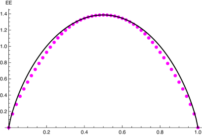
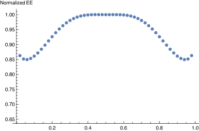
Figure 1: In this figure we present the EE for an excited state with two magnons in the $SU(2)$ sector. On the left part of the figure it is the plot of the EE as a function of the position that we split the spin chain in two parts, $D$ and its complement $D^{C}$. In order to simplify notation and to be able to compare spin chains with different number of sites we normalize the horizontal axis and plot with respect to the ratio of the splitting point divided by the length of the spin chain. In all the subsequent plots of the EE the horizontal axis will be in units of this “normalized splitting” ($N/L$). The black curve is twice the EE of a single magnon while the magenta dots represent the actual computation of the EE, using (2), when the scattering of the two magnons is taken into account. On the right part of the figure, in order to illustrate the saturation points, we present the normalized EE (i.e. dividing (2) by twice the EE of a single magnon). The calculations are for mode number $n=1$ & the length of the spin chain is set to $L=100$.

Given the general expressions for the Renyi Entropy (2) and the EE (2), we are now in position to plot the EE as a function of the size of the part of the spin chain we cut. In figure 1 we present the EE for an excited state with two magnons in the $SU(2)$ sector. The quantum number specifying the momenta of the magnons is set to $n=1$. On the left part of the figure one can see the plot of the EE as a function of the position that we split the spin chain in two parts, $D$ and its complement $D^{C}$. In the same plot we have also drawn twice the EE of a single magnon, which is the upper bound for the EE of any state involving two magnons. One can see that the bound is almost saturated at two symmetric points, one on the left and one on the right of the middle of the chain (see also the right part of Figure 8). To illustrate this point we present the normalised EE, that is the ratio of (2) over twice the EE of the single magnon, on the right part of the figure 1.

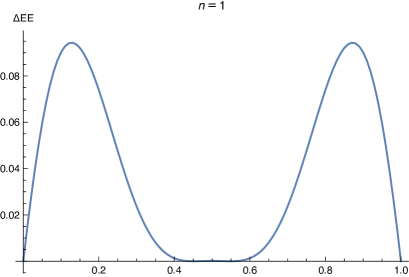
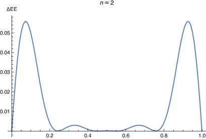
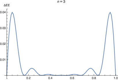
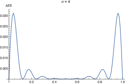
Figure 2: In this figure we present the difference between the EE of two magnons and twice the EE of one magnon when we change/increase the mode number (from mode number one to four), in the $SU(2)$ sector.

In figure 2 we present the dependence of the difference between the aforementioned bound and the EE of two magnon excited state on the mode number $n$, which characterises the excited state. Generically, as one moves towards the centre of the chain the difference oscillates with an amplitude that decreases. Furthermore, as one increases the mode number from one to four the bound is almost saturated for specific values of the length of the domain $D$ for which the EE is calculated. If we exclude the trivial cases where $D$ is either the empty set or when $D$ is the whole chain the number of points that the bound is almost saturated is $2n$ (see also the end of the next paragraph), which is twice the excitation number. We should note that part of the results of the current section have some overlap with the analysis in Molter:2014hna .

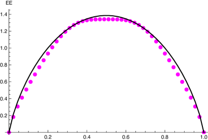
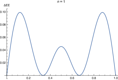
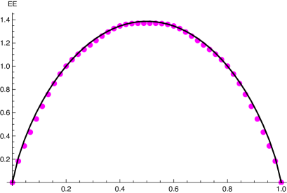
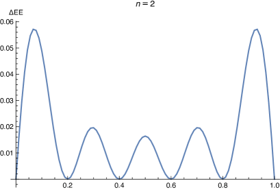
Figure 3: In this figure we present the EE for an excited state with two magnons in the $SU(1|1)$ sector. On the upper left part of the figure it is the plot of the EE as a function of the “normalised splitting” ($N/L$) and on the upper right part the difference between the EE of two magnons and twice the EE of the single magnon again as a function of the “normalised splitting”, when the mode number is $n=1$. In the lower two plots of the figure we present the results for mode number $n=2$, to illustrate the increase of the number of the explicit saturation points when the mode number increases. The black curve is twice the EE of a single magnon while the magenta dots represent the computation of the EE using (2). The length of the spin chain is set to $L=90$.

Looking at the expression of the EE bound (see (2.7) multiplied by two) it is clear that if there points where this bound is explicitly saturated, then the analytic expression of the EE (2) at those points should be independent of the value of the momentum of the excitation. To detect those points, one should go to (2) where all the ingredients are defined and look for a systematic way to eliminate the presence of the momentum. Setting $S_{1}$ and $\hat{S}_{1}$ to zero satisfies the above requirement and furthermore eliminates the presence of the momentum in the expression of $f_{p}$ and $\psi_{D}$. In that way the EE at those points, which simultaneously set to zero $S_{1}$ and $\hat{S}_{1}$, explicitly saturate the bound (2.8). Combining the expressions for $S_{1}$ and $\hat{S}_{1}$ together with the value of the momentum for each one of the three sectors, it is easy to conclude that the bound is explicitly saturated only in the $SU(1|1)$ sector and in the following points

$$\frac{N}{L}\,=\,\frac{\kappa}{2n+1}\quad{\rm with}\quad n\geq 0\quad\&\quad 0\leq\kappa\leq 2n+1.$$ (2.26)

To illustrate the above claim we have plotted in figure 3 the EE in the $SU(1|1)$ sector for two different quantum numbers, namely $n=1$ and $n=2$, in a spin chain with 90 sites. According to (2.26) we expect to have four and six saturation points, located at the positions $(0,1/3,2/3,1)$ and $(0,1/5,2/5,3/5,4/5,1)$ respectively, and this is exactly what we observe in figure 3. In the other two sectors the quantities $S_{1}$ and $\hat{S}_{1}$ can never be simultaneously zero and for that reason the entropy comes very close to the bound but without saturating it. In cases with more than two magnons the existence of saturation points seems difficult to occur, since more than two constraints have to be satisfied simultaneously, but needs to be checked with an explicit calculation.

A final comment concerns the expected fact that the plots for the EE are symmetric with respect to the centre of the spin chain. This is a consequence of the well-known fact that the EE’s of $D$ and of its complementary $D^{C}$ are equal $S_{EE}(D)=S_{EE}(D^{C})$, when the state which describes the system as a whole $D\cup D^{C}$ is a pure state.

The aim of the next section will be to analyse the effect of interactions to the EE. To this end we will focus on the BMN limit of $AdS_{5}\times S^{5}$ and find the exact, in the coupling, expression for the EE.

3 All-loop Entanglement and Renyi Entropies of the superconformal primary operator with two excitations in the BMN limit

One of the most interesting limits of the AdS/CFT correspondence is the so-called BMN limit Berenstein:2002jq . The reason is that in this limit, known as the Penrose or pp-wave limit on the gravity side, the Green-Schwarz superstring action for type IIB strings becomes quadratic in the light-cone variables and as a result one can solve for the superstring spectrum exactly. This result provides an all-orders prediction for the anomalous dimensions of certain operators with large R-charge Beisert:2005tm which are dual to the string states propagating in the pp-wave background. Subsequently, one can study the dynamics of the theory by employing string field theory to construct the three-string vertex (see Lee:2004cq ; Dobashi:2004nm ; Chu:2002pd and references therein) and compare the so-obtained string amplitudes to the corresponding three-point correlators Georgiou:2003aa ; Georgiou:2004ty ; Georgiou:2009tp .

3.1 The superconformal primary operator with two impurities in the BMN limit

In this subsection, we will briefly review the construction of the superconformal primary state involving two excitations (impurities) on both the string and gauge theory side. The full supermultiplet based on this primary state was constructed in Beisert:2002tn at leading order in the coupling expansion. In what follows, we will closely follow Georgiou:2008vk ; Georgiou:2009tp . The main idea is to use the action of the superalgebra on the states of the theory in order to resolve the operator mixing appearing in the wavefunction of the primary operator. More precisely, consider the non-BPS highest weight state (HWS) with two impurities which we will denote by ${\cal O}_{n}$. By definition this state should be annihilated by the sixteen superconformal generators preserved by the pp-wave background. Schematically one has

$$[S,{\cal O}_{n}(x=0)]=0~{}~{}~{}~{}~{}\mbox{and}~{}~{}~{}~{}~{}[Q,{\cal O}_{n}(x=0)]\not=0~{}.$$ (3.27)

The action of the remaining sixteen supersymmetry generators, collectively denoted here by $Q$, on the HWS generates the whole supermultiplet with two impurities. Equation (3.27) should be implemented order by order in perturbation theory since the superconformal charges receive quantum corrections Georgiou:2008vk ; Georgiou:2009tp . However in the pp-wave limit the 32 supercharges can be straightforwardly constructed order by order in the string coupling. What is important for us is that their leading in $g_{s}$ expressions are known to all-orders in the effective Yang-Mills coupling $\lambda^{\prime}=\frac{g_{YM}^{2}N}{J^{2}}$. Here $g_{YM}^{2}N$ is the ’t Hooft coupling while $J$ is the large R-charge of the operator which correspond to the angular momentum of the point-like string orbiting around one of the equators of the five-sphere $S^{5}$ of the parent $AdS_{5}\times S^{5}$ background. Demanding that the full set of the 16 superconformal charges annihilates the HWS one can determine the form of the latter to all orders in $\lambda^{\prime}$. The details of this construction can be found in Georgiou:2008vk . The result for the two-impurity HWS reads

$$|n\rangle=\frac{1}{4(1+U_{n}^{2})}\Bigg{[}{a^{\dagger}}_{n}^{i^{\prime}}{a^{\dagger}}_{n}^{i^{\prime}}\,+\,{a^{\dagger}}_{-n}^{i^{\prime}}{a^{\dagger}}_{-n}^{i^{\prime}}+2U_{n}b_{-n}^{\dagger}\,\Pi\;b_{n}^{\dagger}-U_{n}^{2}\left({a^{\dagger}}_{n}^{i}{a^{\dagger}}_{n}^{i}\,+\,{a^{\dagger}}_{-n}^{i}{a^{\dagger}}_{-n}^{i}\right)\Bigg{]}|\alpha\rangle\,.$$ (3.28)

In (3.28) ${a^{\dagger}}_{\pm n}^{i^{\prime}}$, $b_{\pm n}^{\dagger}$ and ${a^{\dagger}}_{\pm n}^{i}$ denote the creation operators for the four scalar, eight fermionic and four vector excitations while $|\alpha\rangle$ denotes the string vacuum of fixed light-cone momentum $p^{+}$. Furthermore, $n$ is the mode number characterising the excited state while the function $U_{n}$ is given by

$$U_{n}\equiv\frac{1-\rho_{n}}{1+\rho_{n}}\quad{\rm with}\quad\rho_{n}\,=\,\frac{\omega_{n}\,-\,n}{\mu\,\alpha}\quad\&\quad\omega_{n}\,=\,\sqrt{n^{2}\,+\,\left(\mu\,\alpha^{\prime}\,p^{+}\right)^{2}}\,,$$ (3.29)

where $p^{+}$ is the light cone momentum of the state and $\mu$ is the parameter setting the scale of the curvature of the PP-wave background (as usual, $\alpha\equiv\alpha^{\prime}p^{+}$ and $\lambda^{\prime}=1/(\mu\alpha)^{2}$). Finally, $\Pi$ is the appropriate $16\times 16$ block of the matrix $\Pi=\prod_{i^{\prime}=1}^{4}\Gamma^{i^{\prime}}$. The index $i^{\prime}$ takes values in the flavour $SO(4)\subset SO(6)$ and the $\Gamma$ indicate the $SO(1,9)$ gamma matrices.

One important comment is in order. Notice that the HWS string state, as well as the corresponding field theory operator ${\cal O}_{n}$, exhibits the important feature of mixing between different kinds of excitations, namely bosonic and fermionic states (operators) mix among each other as long as the mixing states have the same quantum numbers.

Needless to say that this construction can be generalised to HWS with more than two impurities.

3.2 Exact in $\lambda^{\prime}$ Entanglement Entropy

Our aim in this section is to derive, based on (3.28), an analytic expression for the EE of the two impurity primary operator which is exact in the BMN coupling $\lambda^{\prime}$. This expression will be an interpolating function from the weak coupling regime $\lambda^{\prime}\rightarrow 0$ to the strong coupling regime $\lambda^{\prime}\rightarrow\infty$. We should stress that our result is exact in the strict BMN limit and generically will receive $1/J$ corrections. It would be interesting to calculate these corrections by going to the near-BMN limit.

The first step towards this end is to rewrite (3.28) as an operator of ${\cal N}=4$ SYM. An important observation is that due to mixing of different kinds of impurities this operator can not be restricted in one of the closed subsectors of ${\cal N}=4$ SYM but ”lives” in the full $PSU(2,2|4)$ superalgebra. The field theory operator which is dual to the string state (3.28) can be written as follows

$$(1+U_{n}^{2}){(\mathcal{O}_{st})}^{J}_{n} =\sqrt{\frac{N_{0}^{-J-2}}{J+3}}\,\sum_{i=1}^{2}\sum_{p=0}^{J}\,\cos{\frac{\pi n(2p+3)}{J+3}}\,\text{Tr}\big{[}Z_{i}\,Z^{p}\,\bar{Z}_{i}\,Z^{J-p}\big{]}$$

$$-2\,\sqrt{\frac{N_{0}^{-J-2}}{J+3}}\cos{\frac{\pi n}{J+3}}\,\text{Tr}\big{[}\bar{Z}\,Z^{J+1}\big{]}$$ (3.30)

$$+\frac{U_{n}}{2}\,\sqrt{\frac{N_{0}^{-J-1}}{J+1}}\,\sum_{p=0}^{J-1}\sin{\frac{\pi n(2p+2)}{J+1}}\,\text{Tr}\big{[}\psi^{1\alpha}\,Z^{p}\,\psi^{2}_{\alpha}\,Z^{J-p-1}\big{]}$$

$$-\frac{U_{n}}{2}\,\sqrt{\frac{N_{0}^{-J-1}}{J+1}}\,\sum_{p=0}^{J-1}\sin{\frac{\pi n(2p+2)}{J+1}}\,\text{Tr}\big{[}\bar{\psi}_{3\dot{\alpha}}\,Z^{p}\,\bar{\psi}_{4}^{\dot{\alpha}}\,Z^{J-p-1}\big{]}$$

$$\,-\,\frac{U_{n}^{2}}{4}\,\sqrt{\frac{N_{0}^{-J}}{J-1}}\sum_{p=0}^{J-2}\cos{\frac{\pi n(2p+1)}{J-1}}\,\text{Tr}\big{[}D_{\mu}Z\,Z^{p}\,D^{\mu}\,Z\,Z^{J-p-2}\big{]}\,.$$

In (3.2) $\psi^{A}$ (with $A=1,2,3,4$) denote the four fermions of ${\cal N}=4$ SYM while $\alpha=1,2$ and $\dot{\alpha}=1,2$ are spinor indices over which we sum. Furthermore, $N_{0}=\frac{N}{8\pi^{2}}$ where $N$ is the number of colours. We should mention that in order to translate the string state (3.28) to the field theory operator (3.2) we have used the prescription of Georgiou:2008vk . Namely, we have used the following dictionary

$$\frac{1}{4}\left[{a^{\dagger}}_{n}^{i^{\prime}}\,{a^{\dagger}}_{n}^{i^{\prime}}\,+\,{a^{\dagger}}_{-n}^{i^{\prime}}\,{a^{\dagger}}_{-n}^{i^{\prime}}\right]|\,\alpha\rangle\,\leftrightarrow\,\mathcal{O}^{(0)J}_{n}\,,$$ (3.31)

where $\mathcal{O}^{(0)J}_{n}$ is the sum of the first two terms on the r.h.s. of (3.2). The string state on the l.h.s. of (3.31) is normalised to one and the same is true for the tree-level 2-point function of the corresponding gauge theory operator. In a similar fashion the term with the fermionic oscillators in (3.28) corresponds to a field theory operator with four fermions

$$\frac{1}{2}\left[{b^{\dagger}}_{-n}\,\Pi\,{b^{\dagger}}_{n}\right]|\,\alpha\rangle\,\leftrightarrow\,\mathcal{O}^{(1)J}_{n}\,,$$ (3.32)

where $\mathcal{O}^{(1)J}_{n}$ is the sum of the third and fourth terms on the r.h.s. of (3.2) multiplied by $U_{n}$. Finally, for the term involving the vector impurities we have

$$\frac{1}{4}\left[{a^{\dagger}}_{n}^{i}\,{a^{\dagger}}_{n}^{i}\,+\,{a^{\dagger}}_{-n}^{i}\,{a^{\dagger}}_{-n}^{i}\right]|\,\alpha\rangle\,\leftrightarrow\,\mathcal{O}^{(2)J}_{n}\,,$$ (3.33)

where $\mathcal{O}^{(2)J}_{n}$ is the last term on the r.h.s. of (3.2) multiplied by $U_{n}^{2}$. As in the purely scalar operator, (3.32) and (3.33) are derived so that both the string state and the gauge theory operator are normalised to one. Since the two-point functions of operators involving fermions or/and vector impurities have non-trivial space-time structure we have used the prescription of Georgiou:2004ty ; Georgiou:2003kt . Once is given an operator it is possible to define the barred one, which is the conjugate of the initial operator followed by an inversion. It is then this operator which is used in the calculation of the two-point function. This prescription is motivated by the radial quantisation in two-dimensional CFT’s and results to two-point functions which can be easily normalised to one.

One can now use the following relation

$$\sum_{p=0}^{J}\cos{\frac{\pi n(2p+3)}{J+3}}\,\text{Tr}\big{[}X\,Z^{p}\,Y\,Z^{J-p}\big{]}\,\approx\,\frac{1}{2\,J}\times$$ (3.34)

$$\sum_{1\leq x_{1}<x_{2}\leq J}\left(e^{i(p_{1}x_{2}\,+\,p_{2}x_{1})}\,+\,e^{i(p_{1}x_{1}\,+p_{2}x_{2})}\right)\,\text{Tr}\big{[}Z^{x_{1}-1}\,X\,Z^{x_{2}-x_{1}-1}\,Y\,Z^{J-x_{2}}\big{]}\,,$$

as well as the analogous equation for the fermionic term to rewrite (3.2) as a spin chain wavefunction. To achieve this one should take into account the fact that $p_{1}=p=-p_{2}=2\pi n/J<<1$ and as a result to leading order in the large $J$ expansion $e^{\pm ip}\approx 1$ and $\cos\big{(}{\pi n/(J+3)}\big{)}\approx 1$. Furthermore, we will make use of the following correspondence between the Yang-Mills and spin chain excitations Georgiou:2012zj

$$\frac{1}{\sqrt{N_{0}}}\,Z_{YM}\leftrightarrow Z_{sp}\qquad\frac{1}{\sqrt{2\,N_{0}}}\,\psi^{A}_{YM}\leftrightarrow\psi^{A}_{sp}\qquad\frac{1}{\sqrt{2\,N_{0}}}\,\left(D_{\mu}Z\right)_{YM}\leftrightarrow\left(D_{\mu}Z\right)_{sp}\,.$$ (3.35)

In conclusion the wavefunction of the non-BPS primary operator with two excitations can be written in the spin chain language as (we suppress the index ”sp” since from now on we will be using only the spin chain wavefunctions) follows

$$|\psi\rangle = \frac{\mathcal{N}}{2J}\,\Bigg{[}\sum_{i=1}^{2}\sum_{x_{1}<x_{2}}\left(e^{ip_{1}x_{2}+ip_{2}x_{1}}+e^{ip_{1}x_{1}+ip_{2}x_{2}}\right)|(Z_{i})_{x_{1}}({\bar{Z}}_{i})_{x_{2}}\rangle\,-\,4\sum_{x}|{\bar{Z}}_{x}\rangle$$

$$- i\,U_{n}\sum_{x_{1}<x_{2}}\left(e^{ip_{1}x_{2}+ip_{2}x_{1}}-e^{ip_{1}x_{1}+ip_{2}x_{2}}\right)\left(|(\psi^{1\alpha})_{x_{1}}(\psi^{2}_{\alpha})_{x_{2}}\rangle-|({\bar{\psi}}_{3\dot{\alpha}})_{x_{1}}({\bar{\psi}}_{4}^{\dot{\alpha}})_{x_{2}}\rangle\right)$$

$$- \frac{U_{n}^{2}}{2}\sum_{x_{1}<x_{2}}\left(e^{ip_{1}x_{2}+ip_{2}x_{1}}+e^{ip_{1}x_{1}+ip_{2}x_{2}}\right)|(D_{\mu}Z)_{x_{1}}(D^{\mu}Z)_{x_{2}}\rangle\Bigg{]}\,.$$

A couple of important comments are in order. As is stressed in Beisert:2005tm the ${\cal N}=4$ SYM spin chain is dynamic in the sense that the length of the chain in not fixed since different impurities have different scaling dimensions. Indeed as can be seen from (3.2) the number of $Z$ fields is not the same in all terms. We should mention that each of the kets written in (3.2) describe two excitations in the appropriate number of $Z$ fields dictated by (3.2). The dynamic nature of the spin chain may result to a situation where both vector impurities lie in the domain $D$ but the scalar impurities lie on in $D$ and one in its complementary. This can happen when both excitations are close to the boundary of $D$. In what follows we will ignore such circumstances since their contribution will be $1/J$ suppressed in the BMN limit. As second related comment concerns the exact form of (3.2). As is well-known the exact expression for the eigenstate of the dilatation operator will have non-asymptotic terms where the two impurities will be close to each other. As it happens with the two-point functions one can show that these terms give a contribution which is also $1/J$ suppressed with respect to the contributions coming from the asymptotic terms and as such can be ignored in the strict BMN limit where $J\rightarrow\infty$. Finally, let us notice that the state (3.2) may, in principle, be taken from considering the scattering of two scalar impurities with a double copy of the $SU(2|2)$ scattering matrix of Beisert:2005tm .

We are now in position to write down the RDM originating from the wavefunction above. As usual we will be cutting the spin chain into two parts. One part is from site 1 to site $N$, which is the domain $D$ of which the EE we intend to calculate, while the remaining part is the complementary $D^{C}$ whose degrees of freedom we have to trace out in order to obtain the RDM. Furthermore, as in the case of two magnons at weak coupling (see section 2) by $|\psi_{D}\rangle$ we denote the wavefunction of the part $D$ when both magnons sit in the region $D$, while by $|\psi_{D}^{C}\rangle$ we denote the wavefunction of the complementary region $D^{C}$ when both magnons sit in the region $D^{c}$. After these explanations the RDM can be written as

$$\rho_{D} = \kappa\,\Bigg{[}|\psi_{D}\rangle\langle\psi_{D}|\,+\,|\downarrow\rangle_{D\,\,\,D}\langle\downarrow|\,\,\,\,f_{p}\,+4^{2}\left(\sum_{x}|(\bar{Z})_{x}\rangle\langle(\bar{Z})_{x}|\,+\,|\downarrow\rangle_{D\,\,\,D}\langle\downarrow|(J-N)\right)$$ (3.37)

$$+ \sum_{x_{1}<x^{\prime}_{1}}\,\Bigg{(}\sum_{i=1}^{2}|(Z_{i})_{x_{1}}\rangle\langle(Z_{i})_{x^{\prime}_{1}}|\,\,\,\,g_{p}^{(1)}(x_{1},x^{\prime}_{1})+|(\psi^{1\alpha})_{x_{1}}\rangle\langle(\psi^{1\alpha})_{x^{\prime}_{1}}|\,\,\,\,g_{p}^{(2)}(x_{1},x^{\prime}_{1})$$

$$+ |(\psi_{3\dot{\alpha}})_{x_{1}}\rangle\langle(\psi_{3\dot{\alpha}})_{x^{\prime}_{1}}|\,\,\,\,g_{p}^{(2)}(x_{1},x^{\prime}_{1})+|(D_{\mu}Z)_{x_{1}}\rangle\langle D_{\mu}Z)_{x^{\prime}_{1}}|\,g_{p}^{(3)}(x_{1},x^{\prime}_{1})\Bigg{)}\Bigg{]}\,,$$

where

$$g_{p}^{(1)}\,=\,g_{p}^{SU(2)}\quad{\rm with}\quad S_{SU(2)}(p_{2},p_{1})\,=\,1\,,$$

$$g_{p}^{(2)}=U_{n}^{2}g_{p}^{SU(1|1)}\quad{\rm with}\quad S_{SU(1|1)}(p_{2},p_{1})\,=\,-\,1\,,$$ (3.38)

$$g_{p}^{(3)}=\frac{U_{n}^{4}}{4}g_{p}^{SU(2)}\quad{\rm with}\quad S_{SL(2)}(p_{2},p_{1})\,=\,1\,,$$

that is $g_{p}^{(1)}$ is the same function appearing in the weak coupling calculation of section 2 but with the scattering matrix set to one and so on. We should mention that the fact that the scattering matrices should be set to $\pm 1$ is in accordance with the standard lore that in the BMN limit the impurities do not scatter at all since they are most of the time very far from each other.

It is now straightforward to write down the n-th power of the RDM

$$\rho_{D}^{\eta} =\,\kappa^{\eta}\,\Bigg{[}|\psi_{D}\rangle\langle\psi_{D}|\langle\psi_{D}|\psi_{D}\rangle^{\eta-1}\,+\,|\downarrow\rangle_{D\,\,\,D}\langle\downarrow|\,\,f_{p}^{\eta}$$

$$+\,4^{2\eta}\left(N^{\eta-1}\sum_{x}|(\bar{Z})_{x}\rangle\langle(\bar{Z})_{x}|\,+\,\left(J\,-\,N\right)^{\eta}\,|\downarrow\rangle_{D\,\,\,D}\langle\downarrow|\right)$$ (3.39)

$$+\,\sum_{x_{1}<x^{\prime}_{1}}\,\Bigg{(}\sum_{i=1}^{2}|(Z_{i})_{x_{1}}\rangle\langle(Z_{i})_{x^{\prime}_{1}}|\,\,\sum_{y_{1},...,y_{\eta-1}\in D}g_{p}^{(1)}(x_{1},y_{1})g_{p}^{(1)}(y_{1},y_{2})...g_{p}^{(1)}(y_{\eta-1},x^{\prime}_{1})$$

$$+\,|(\psi^{1\alpha})_{x_{1}}\rangle\langle(\psi^{1\alpha})_{x^{\prime}_{1}}|\,\,\,\,\sum_{y_{1},...,y_{\eta-1}\in D}g_{p}^{(2)}(x_{1},y_{1})g_{p}^{(2)}(y_{1},y_{2})...g_{p}^{(2)}(y_{\eta-1},x^{\prime}_{1})$$

$$+\,|(\psi_{3\dot{\alpha}})_{x_{1}}\rangle\langle(\psi_{3\dot{\alpha}})_{x^{\prime}_{1}}|\,\,\,\,\sum_{y_{1},...,y_{\eta-1}\in D}g_{p}^{(2)}(x_{1},y_{1})g_{p}^{(2)}(y_{1},y_{2})...g_{p}^{(2)}(y_{\eta-1},x^{\prime}_{1})$$

$$+\,|(D_{\mu}Z)_{x_{1}}\rangle\langle D_{\mu}Z)_{x^{\prime}_{1}}|\,\sum_{y_{1},...,y_{\eta-1}\in D}g_{p}^{(3)}(x_{1},y_{1})g_{p}^{(3)}(y_{1},y_{2})...g_{p}^{(3)}(y_{\eta-1},x^{\prime}_{1})\Bigg{)}\Bigg{]}\,.$$

A couple of comments are in order. The first term in the first line of (3.2) originates from the partition where both magnons are in the region $D$, while the second term from the partition where both magnons are in the complementary region $D^{C}$. Furthermore, the second line of (3.2) comes from part of the wavefunction which has a single impurity $\bar{Z}$. Finally, the rest of the expression originates from the partition where one of the magnons is in the region $D$ and one in the complementary $D^{C}$.

The next step is to find the exact in $\lambda^{\prime}$ Renyi Entropy

$$S^{(\eta)}_{R} = \frac{1}{1\,-\,\eta}\,\log{Tr_{D}\,\rho_{D}^{\eta}}\qquad{\rm with}$$ (3.40)

$$Tr_{D}\rho_{D}^{\eta}\, = \,\kappa^{\eta}\,\Bigg{[}\langle\psi_{D}|\psi_{D}\rangle^{\eta}+f_{p}^{\eta}+\left(2^{\eta}+\left(U_{n}^{4}\right)^{\eta}\right)\,\left[\left(A^{(1)}+A^{(1)*}\right)N+B^{(1)}\,\hat{S}_{1}^{*}+B^{(1)*}\hat{S}_{1}\right]$$

$$+ \left(4U_{n}^{2}\right)^{\eta}\,\left[\left(A^{(2)}+A^{(2)*}\right)N+B^{(2)}\hat{S}_{1}^{*}+B^{(2)*}\hat{S}_{1}\right]+4^{2\eta}\left(N^{\eta}+\left(J-N\right)^{\eta}\right)\Bigg{]}\,,$$

where all quantities are defined in section 2. We should only add that $A^{(1)}=A^{SU(2)}$ and $B^{(1)}=B^{SU(2)}$ are the $SU(2)$ weak coupling expressions for $A$ and $B$ defined in section 2 but with $SU(2)$ scattering matrix set to one, i.e. $S_{SU(2)}(p_{2},p_{1})=1$. Similarly, $A^{(2)}=A^{SU(1|1)}$ and $B^{(2)}=B^{SU(1|1)}$ are the $SU(1|1)$ weak coupling expressions for $A$ and $B$ defined in section 2 but with $SU(1|1)$ scattering matrix set to minus one, i.e. $S_{SU(1|1)}(p_{2},p_{1})=-1$. Before we continue with the $\eta\rightarrow 1$ limit and the calculation of the EE, we would like to comment on the coefficients of the different contributions in (3.40) (namely scalar, fermion and vector) and their $\eta$ dependence.

The second line of (3.2) gives the last term in (3.40). The third line of (3.2) gives the part of the third term in (3.40) which is proportional to $2^{\eta}$. This happens since $i=1,2$ so we have to raise two to the $\eta$-th power, i.e $2^{\eta}$. The fourth and fifth lines of (3.2) give the penultimate term in (3.40). Since $\alpha=1,2$ and ${\dot{\alpha}}=1,2$ we have to multiply $U_{n}$ by four and then raise to the $\eta$-th power, i.e $\left(4\times U_{n}^{2}\right)^{\eta}$. In the same fashion, since $\mu=1,2,3,4$, the ultimate term in (3.2) has to be multiplied by four and then raised to the $\eta$-th power, i.e. $\left(4\times\frac{U_{n}^{4}}{4}\right)^{\eta}$ to give the part of the third term of (3.40) that is proportional to $U_{n}^{4\eta}$.

Taking the limit $\eta\rightarrow 1$ we find for the EE of the two magnon excited state

$$S_{EE} =\,-\,\kappa\,\Bigg{[}16\Big{[}N\log{(16N)}\,+\,\left(J-N\right)\,\log{\big{(}16\left(J-N\right)\big{)}}\Big{]}\,+\,f_{p}\,\log{f_{p}}$$

$$+\,\langle\psi_{D}|\psi_{D}\rangle\,\log{\langle\psi_{D}|\psi_{D}\rangle}\,+\,\Bigg{(}4U_{n}^{2}\sum_{i=1}^{2}G_{i}^{(2)}\,\log{(4\,U_{n}^{2}\,\lambda_{i}^{(2)})}$$ (3.41)

$$+\,2\sum_{i=1}^{2}G_{i}^{(1)}\,\log{(2\,\lambda_{i}^{(1)})}\,+\,U_{n}^{4}\sum_{i=1}^{2}G_{i}^{(1)}\,\log{(U_{n}^{4}\,\lambda_{i}^{(1)})}\,+\,c.c.\Bigg{)}\Bigg{]}\,+\,\log{\kappa}\,,$$

where in full analogy with (2)

$$G_{1}^{(i)}\,=\,\frac{-\,\beta^{(i)*}}{2\,\sqrt{\Delta^{(i)}}}\,\left(A^{(i)}\,-\,U_{12}^{(i)}\,B^{(i)*}\right)\left(U_{11}^{(i)}\,N\,+\,\hat{S}_{1}\right)\,\,\&\quad U_{11}^{(i)}\,=\,\frac{i\,Im\,\alpha^{(i)}\,-\,\sqrt{\Delta^{(i)}}}{\beta^{(i)*}}$$

$$G_{2}^{(i)}\,=\,\frac{\beta^{(i)*}}{2\sqrt{\Delta^{(i)}}}\,\left(A^{(i)}\,-\,U_{11}^{(i)}\,B^{(i)*}\right)\left(U_{12}^{(i)}\,N\,+\,\hat{S}_{1}\right)\,\,\&\quad U_{12}^{(i)}\,=\,\frac{i\,Im\,\alpha^{(i)}\,+\,\sqrt{\Delta^{(i)}}}{\beta^{(i)*}}$$ (3.42)

$$\lambda_{1}^{(i)}\,=\,Re\,\alpha^{(i)}\,-\,\sqrt{\Delta^{(i)}}\,,\quad\lambda_{2}^{(i)}=Re\alpha^{(i)}+\sqrt{\Delta^{(i)}}\quad{\rm with}\quad\Delta^{(i)}\,=\,-(Im\,\alpha^{(i)})^{2}\,+\,|\beta^{(i)}|^{2}\,.$$

The upper index $i=1$ denotes that the quantities that carry it are defined in the $SU(2)$ sector with the scattering matrix set to one. Similarly, when the upper index $i$ is set to two, $i=2$, denotes quantities as defined in the $SU(1|1)$ sector with the scattering matrix set to minus one. Finally, the expressions for the inner products in (3.40) & (3.2) are

$$\langle\psi|\psi\rangle\,=\,2\langle\psi|\psi\rangle^{SU(2)}\,+\,16J\,+\,4U_{n}^{2}\langle\psi|\psi\rangle^{SU(1|1)}\,+\,U_{n}^{4}\langle\psi|\psi\rangle^{SU(2)}$$

$$\langle\psi_{D}|\psi_{D}\rangle\,=\,2\langle\psi_{D}|\psi_{D}\rangle^{SU(2)}\,+\,4U_{n}^{2}\langle\psi_{D}|\psi_{D}\rangle^{SU(1|1)}\,+\,U_{n}^{4}\langle\psi_{D}|\psi_{D}\rangle^{SU(2)}$$ (3.43)

$$f_{p}\,=\,2\langle\psi_{D^{C}}|\psi_{D^{C}}\rangle^{SU(2)}\,+\,4U_{n}^{2}\langle\psi_{D^{C}}|\psi_{D^{C}}\rangle^{SU(1|1)}\,+\,U_{n}^{4}\langle\psi_{D^{C}}|\psi_{D^{C}}\rangle^{SU(2)}\,,$$

where $\langle\psi|\psi\rangle^{SU(2)}$ and $\langle\psi|\psi\rangle^{SU(1|1)}$ denote the inner product for the eigenstate of the one-loop dilatation operator in the $SU(2)$ and $SU(1|1)$ sectors, respectively. These are defined in section 2.

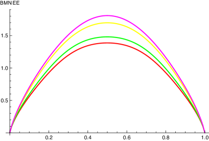
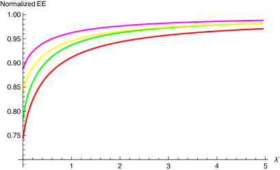
Figure 4: In this figure we present the EE for an excited state with two magnons in the BMN limit. The mode number of the state is taken to be $n=1$. On the left part of the figure it is the plot of the EE as a function of the normalised splitting of the spin chain, for different values of $\lambda^{\prime}$. The correspondence between colour and $\lambda^{\prime}$ is the following: Red $\Rightarrow$ $\lambda^{\prime}=0$, Green $\Rightarrow$ $\lambda^{\prime}=0.1$, Yellow $\Rightarrow$ $\lambda^{\prime}=1$ & Magenta $\Rightarrow$ $\lambda^{\prime}=5$. On the right part of the figure we present the EE flow from the IR (lower values of $\lambda^{\prime}$) to the UV (higher values of $\lambda^{\prime}$) as we change the splitting point of the spin chain. In order to compare the different curves we have normalised each one by dividing with the EE for $\lambda^{\prime}\rightarrow\infty$. In this way all the curves approximate to one. The correspondence between colours and normalised splitting (e.g. $N/L$) of the spin chain is the following: Red $\Rightarrow$ $0.5$, Green $\Rightarrow$ $0.1$, Yellow $\Rightarrow$ $0.01$ & Magenta $\Rightarrow$ $0.001$.

Now having at hand the analytic expressions for both the Renyi entropy (3.40) and the EE (3.2), we will probe the parametric space and extract interesting qualitative behaviours. As can be seen from both (3.40) & (3.2) both quantities depend on the position we split the spin chain in two parts ($D$ and its complement $D^{C}$), the coupling constant $\lambda^{\prime}$ and the mode number $n$ characterising the excited state. In figure 4 we present the EE for an excited state with $n=1$ in the BMN limit. On the left part of the figure it is the plot of the EE as a function of the normalised splitting of the spin chain, for different values of $\lambda^{\prime}$. As can be seen from the plot (the correspondence colour/$\lambda^{\prime}$ is explained in the caption of the figure) the EE increases as we increase the value of the coupling. To fully realise/visualise this EE flow from the UV to IR, on the right part of figure 4 we present the EE as a function of the coupling $\lambda^{\prime}$, for different values of the splitting point of the spin chain. In order to compare the different curves in a unified manner we have normalised each one by dividing with the EE for $\lambda^{\prime}\rightarrow\infty$, i.e.

$${\rm Normalised}\,S_{EE}(N,\lambda^{\prime},n)\,=\,\frac{S_{EE}(N,\lambda^{\prime},n)}{S_{EE}(N,\infty,n)}\,.$$ (3.44)

Since the EE is related to the central charge of the underlying CFT, this monotonically decreasing behaviour of the EE along the RG flow from $\lambda^{\prime}\rightarrow\infty$ to $\lambda^{\prime}\rightarrow 0$ could be related to the existence of a $c$-theorem Myers:2010xs ; Myers:2010tj , which connects through an RG flow a fixed point in the UV with another fixed point in the IR.

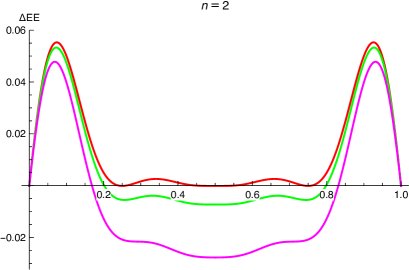
Figure 5: In this figure we present the difference between the EE in the BMN limit and twice the EE of the single magnon (2.7), when we increase the mode number (from mode number one to two), for different values of $\lambda^{\prime}$. For the left plot the correspondence colour/$\lambda^{\prime}$ is Red $\Rightarrow$ $\lambda^{\prime}=0$, Green $\Rightarrow$ $\lambda^{\prime}=0.1$ & Magenta $\Rightarrow$ $\lambda^{\prime}=0.5$, while for the right plot is Red $\Rightarrow$ $\lambda^{\prime}=0$, Green $\Rightarrow$ $\lambda^{\prime}=0.01$ & Magenta $\Rightarrow$ $\lambda^{\prime}=0.05$.

As we pointed out in (2.8) and verified with the calculations of the EE for the three different rank one sectors in section 2, the EE of a single magnon multiplied by the number of impurities (two in our case) appears to be an upper bound for the EE. As can be seen from the two plots of figure 5 this bound is violated as soon as we move away from the $\lambda^{\prime}\rightarrow 0$ limit. In order to underline the violation of this bound for finite $\lambda^{\prime}$ in figure 5 we plot the the difference between the EE in the BMN limit and twice the EE of the single magnon, when we increase the mode number (from mode number one/left to two/right), for different values of $\lambda^{\prime}$. As can be seen from the plots, when the coupling increases it is possible to find pieces of the spin chain with EE that violate the bound and as we increase the value of $\lambda^{\prime}$ more and more pieces acquire EE that violate the bound. Gradually all the pieces of the spin chain will violate the bound and the bigger is the mode number the faster (i.e. with lower value of $\lambda^{\prime}$) this violation will be implemented. The smaller the part of the chain we cut the more we have to increase the value of $\lambda^{\prime}$ to violate the bound. In order to decide if it exists a $\lambda^{\prime}_{crit}$, after which the bound is violated no matter how small is the length of the chain, we need to consider $1/J$ corrections to the EE in (3.2).

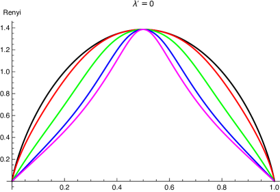
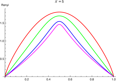
Figure 6: In this figure we present the Renyi entropy in the BMN limit (of different orders) as a function of the normalised splitting, for two values of $\lambda^{\prime}$, $\lambda^{\prime}=0$ and $\lambda^{\prime}=5$. The correspondence between color and Renyi order is the following: Red $\Rightarrow$ $\eta=1$, Green $\Rightarrow$ $\eta=2$, Blue $\Rightarrow$ $\eta=5$ & Magenta $\Rightarrow$ $\eta=10$. The Black curve corresponds to twice the EE of the single magnon. The calculations are for mode number $n=1$.

We close this section with a couple of plots for the Renyi entropy and its dependence on the order $\eta$, $\lambda^{\prime}$ and the normalised splitting $N/L$. In figure 6 we present the Renyi entropy (of different orders) as a function of the normalised splitting, for two values of $\lambda^{\prime}$, $\lambda^{\prime}=0$ and $\lambda^{\prime}=5$. From these two plots it is clear that for finite $\lambda^{\prime}$ the bound is violated for any value of the order parameter $\eta$. Furthermore for two order parameters $\eta_{1}$ & $\eta_{2}$ with $\eta_{1}<\eta_{2}$ the two Renyi entropies $S_{R}^{(\eta_{1})}$ & $S_{R}^{(\eta_{2})}$ obey the inequality $S_{R}^{(\eta_{1})}>S_{R}^{(\eta_{2})}$, making $S_{R}^{(2)}$ a useful lower bound on $S_{R}^{(1)}$. This is a known feature of the Renyi entropy from field theory considerations of its functional dependence on the order parameter, (see e.g. Beck ).

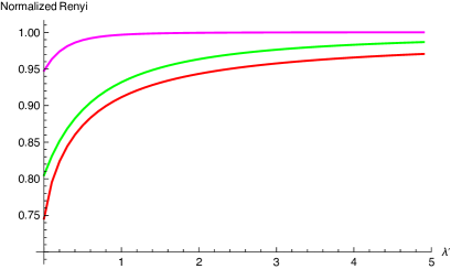
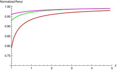
Figure 7: In this figure we present the Renyi entropy flow (of different orders) from the IR (lower values of $\lambda^{\prime}$) to the UV (higher values of $\lambda^{\prime}$), as we change the normalised splitting (left plot $\Rightarrow$ $N/L=0.5$ & right plot $\Rightarrow$ $N/L=0.2$). As in figure 4, we have normalized each of the curves by dividing with the Renyi entropy for $\lambda^{\prime}\rightarrow\infty$. The correspondence between color and Renyi order is the following: Red $\Rightarrow$ $\eta=1$, Green $\Rightarrow$ $\eta=2$ & Magenta $\Rightarrow$ $\eta=10$.

In figure 7 we highlight the flow of the Renyi entropy from the UV to IR (besides that of the EE that we already saw in figure 4). In this figure we present the normalised Renyi entropy (see (3.44) for the definition of this normalisation) flow (of different orders) from the IR (lower values of $\lambda^{\prime}$) to the UV (higher values of $\lambda^{\prime}$), as we change the normalised splitting. From these plots it is clear that increasing the order (or decreasing the length of the spin chain we cut) decreases the difference between the IR and the UV values of the Renyi entropy.

4 Entanglement Entropy from the Algebraic Bethe Ansatz

In this section we concentrate on the case where there is an arbitrary number of excitations (magnons) propagating in the spin chain. In such a case the method used in the previous section for the case of two magnons becomes cumbersome because of the large number of excitations. However, it is the formalism of ABA that comes to rescue in this occasion. Following the same reasoning as before, we split the spin chain of length $L$ in two pieces. The first piece which we call $D$ contains the sites from $1$ to $N$, while its complementary $D^{C}$ contains the sites from $N+1$ to $L$. In the ABA language the wavefunction $|\psi\rangle$ describing the excited state is characterised by a set of $M$ numbers $\{u_{i}\},\,\,i=1,2,...,M$. The $u_{i}$’s are called the rapidities of the $M$ magnons and for an on-shell state they should satisfy the Bethe equations of the corresponding sector. Thus (see Faddeev:1996iy ; Escobedo:2010xs for all the details about the formalism of the ABA),

$$|\psi\rangle\,=\,|\{u_{i}\}\rangle\,=\,\sum_{a\bigcup\bar{a}\,=\,\{u_{i}\}}H(a,\bar{a})\,|a_{l}\rangle\otimes|\bar{a}_{r}\rangle\,,$$ (4.45)

where the sum is over all the possible partitions of the $M$ magnons into two sets. If for example we have two magnons, as in the cases of the CBA we worked so far, the possible partitions are $\left(\{\},\{u_{1},u_{2}\}\right),\left(\{u_{1}\},\{u_{2}\}\right),\left(\{u_{2}\},\{u_{1}\}\right)$ & $\left(\{u_{1},u_{2}\},\{\}\right)$. The set of magnons with rapidities $a_{l}$ are sitting in the left part of the spin chain, that is in region $D$, while the set of magnons with rapidities $a_{r}$ are sitting in the complementary region of the chain, that is $D^{C}$. The function $H(a,\bar{a})$ describes the weight of each partition, it is different in each rank one subsector of the ${\cal N}=4$ SYM and its form is given by (for the various functions appearing in (4.46) see also Appendix A)

$$H(a,\bar{a})\,=\,f^{a\bar{a}}\,d_{r}^{a}\,a_{l}^{\bar{a}}\,.$$ (4.46)

Starting from (4.45) it is now straightforward to evaluate the RDM

$$\rho_{D}\, = \,\kappa\,\sum_{\bar{c}_{r}}\,\sum_{\scriptsize\begin{array}[]{c}a_{l}\cup\bar{a}_{r}\\ b_{l}\cup\bar{b}_{r}\end{array}}\,H(a_{l},\bar{a}_{r})\,H^{*}(b_{l},\bar{b}_{r})\,\langle\bar{c}_{r}|\bar{a}_{r}\rangle\otimes|a_{l}\rangle\langle b_{l}|\otimes\langle\bar{b}_{r}|\bar{c}_{r}\rangle$$ (4.49)

$$= \kappa\,\sum_{m=0}^{M}\,\sum_{a_{l}^{m}\,,\,b^{m}_{l}}f^{(m)}_{a^{m}_{l}b^{m}_{l}}\,\,|a^{m}_{l}\rangle\langle b^{m}_{l}|\,,$$ (4.50)

where we have defined the following quantity

$$f^{(m)}_{a^{m}_{l}b^{m}_{l}}\,\equiv\,H(a^{(m)}_{l},\bar{a}^{(M-m)}_{r})\,H^{*}(b^{(m)}_{l},\bar{b}^{(M-m)}_{r})\,\,\langle\bar{b}^{(M-m)}_{r}|\bar{a}^{(M-m)}_{r}\rangle.$$ (4.51)

In (4.49) $\bar{c}_{r}$ denotes a complete basis of states of the complementary part of the spin chain $D^{C}$. In order to get the last expression for the RDM we have used the completeness relation for the basis $\bar{c}_{r}$

$$\sum_{\bar{c}_{r}}\,\,|\bar{c}_{r}\rangle\langle\bar{c}_{r}|\,=\,I_{r}\,.$$ (4.52)

Here we should stress that because the scalar product of two states involving different numbers of magnons is zero the RDM can be written as a sum of terms each of which has a definite number of excitations $m$ in the region $D$. Subsequently, for each of these terms one has to sum over all possible partitions of the full set of rapidities into two sets, one having $m$ excitations and its complementary having $M-m$ excitations. Notice that the scalar products appearing in the second line of (4.49) are generic off-sell products, since none of the sets of rapidities $\bar{a}_{r}$ nor $\bar{b}_{r}$ satisfy the Bethe equations for the complementary region of the spin chain. This scalar product is given in terms of the recursion relation in equation (A). The normalisation constant $\kappa$ is obtained by demanding the condition

$$Tr_{D}\rho_{D}\,=\,1\qquad\Rightarrow\qquad\kappa^{-1}\,=\,\langle\psi|\psi\rangle\,=\,\sum_{m=0}^{M}\,\sum_{a_{l}^{m}}F^{(m)}_{a^{m}_{l}a^{m}_{l}}\,,$$

$$\text{with}\quad F^{(m)}_{a^{m}_{l}b^{m}_{l}}\,=\,f^{(m)}_{a^{m}_{l}c^{m}_{l}}\,g^{(m)}_{c^{m}_{l}b^{m}_{l}}\qquad{\rm and}\qquad g^{(m)}_{c^{m}_{l}b^{m}_{l}}\,=\,\langle c^{(m)}_{l}|b^{(m)}_{l}\rangle\,.$$ (4.53)

A final comment concerns the dimensionality of the matrices $F^{(m)}$, $f^{(m)}$ and $g^{(m)}$. The dimensionality of each of these square matrices depend on the number $m$ of magnons sitting in the region $D$ and is given by

$$d(m)\,\equiv\,\frac{M!}{m!(M-m)!}\,.$$ (4.54)

As we will see in a while it is the matrices $F^{(m)}$ which one has to diagonalise in order to calculate the EE. As a result the numerical complexity of the calculation grows not with the number of the sites of the region $D$ of which the EE we are after, but like $2^{M}$, that is with the number of magnons running in the spin chain. This advantage is related to the fact that we have employed the powerful technique of the ABA and not that of the CBA.

We are now in position to evaluate the $\eta$-th power of the RDM and take its trace to obtain the Renyi Entropy of the region $D$ as follows

$$\rho^{\eta}_{D}\,=\,\kappa^{\eta}\,\sum_{m=0}^{M}\left[\rho^{(m)}_{D}\right]^{n}\quad{\rm with}\quad\left[\rho^{(m)}_{D}\right]^{\eta}\,=\,\sum_{a^{m}_{l},b^{m}_{l},c^{m}_{l}}|a^{(m)}_{l}\rangle\langle b^{(m)}_{l}|\left[F^{(m)}_{a^{m}_{l}c^{m}_{l}}\right]^{\eta-1}f^{(m)}_{c^{m}_{l}b^{m}_{l}}\Rightarrow$$

$$Tr_{D}\left[\rho_{D}\right]^{\eta}\,=\,\kappa^{\eta}\,\sum_{m=0}^{M}\sum_{a^{m}_{l}}\,\left[F^{(m)}_{a^{m}_{l}a^{m}_{l}}\right]^{\eta}\,.$$ (4.55)

Thus we see that in order to evaluate the Renyi entropy we need to diagonalise the matrices $\kappa\,F^{(m)}$ and sum their eigenvalues after they are raised to the $\eta^{th}$ power. By taking the $\eta\rightarrow 1$ limit of the Renyi entropy it is straightforward to show that the EE is given by

$$S_{EE}\,=\,-\,\sum_{m=0}^{M}\,Tr\Big{[}\kappa\,F^{(m)}\,\log{(\kappa\,F^{(m)})}\Big{]}\,.$$ (4.56)

Thus, as mentioned above, it is enough to diagonalise each of the matrices $\kappa F^{(m)}$. If we denote the eigenvalues of each of these matrices by $\lambda^{(m)}_{i}$ with $i=1,2,\ldots,d(m)$ then the EE of the part $D$ of the spin chain can be finally written as

$$S_{EE}\,=\,-\,\sum_{m=0}^{M}\,\sum_{i=1}^{d(m)}\,\lambda^{(m)}_{i}\,\log{\lambda^{(m)}_{i}}\,.$$ (4.57)

In the final expression (4.57), the EE of each one of the three rank one sectors of ${\cal N}=4$ SYM is a function of the length of the spin chain, the position we split it in two parts ($D$ and its complement $D^{C}$) and the number of excitations (magnons). In figures 8 & 9 we focus on the $SU(2)$ sector of the theory. On the left part of figure 8 we plot the EE of a spin chain with 14 sites as a function of the position of the splitting point. We plot the EE for different number of magnons, from two to seven. At this point we should point out that there is a perfect match of the EE for the two magnons, between the CBA and the ABA calculations (for all the three rank-one subsectors). That is a non-trivial consistency check for the calculations that we present.

The Bethe roots we use in the calculation of the EE are coming after solving the Bethe equation, with the recursive method of Bargheer:2008kj , and distribute themselves along two disjoint cuts on the complex plane. As can be seen from this plot the EE increases as we increase the number of the magnons, but the qualitative behaviour remains the same. It increases as the splitting point approaches the middle of the chain and it is symmetric under the change $N$ (splitting point) $\rightarrow$ $L-N$.

Our initial motivation in employing the very efficient ABA formulation was reaching the thermodynamic limit, by increasing both the number of magnons and the length of the spin chain. However, this is a very complicated numerical task. As we mentioned before, the calculation of the EE for $M$ magnons in a spin chain boils down to diagonalising matrices with dimension $d(m)$. This means that either a very powerful machine is needed or the problem needs to be formulated in a different basis when the number of magnons increases.

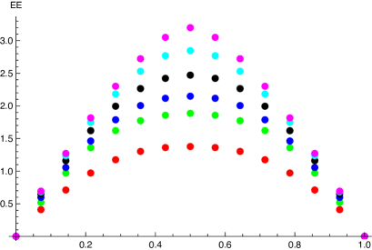
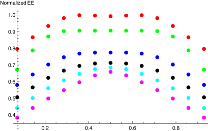
Figure 8: In this figure we present the EE of an excited state in the $SU(2)$ sector. On the left part of the figure it is the plot of the EE as a function of the normalised splitting of the spin chain. On the right part of the figure it is the plot of the normalised EE (i.e. the EE for $M$ magnons divided by $M$ times the EE of one magnon) again as a function of the normalised splitting. The different colours for the bullets in both plots correspond to different number of magnons present in the spin chain. The correspondence between colour and number of magnons is the following: Red $\Rightarrow$ 2 magnons, Green $\Rightarrow$ 3 magnons, Blue $\Rightarrow$ 4 magnons, Black $\Rightarrow$ 5 magnons, Cyan $\Rightarrow$ 6 magnons & Magenta $\Rightarrow$ 7 magnons.

On the right panel of figure 8 we plot the normalised EE (i.e. the EE for $M$ magnons divided by $M$ times the EE of one magnon) again as a function of the position of the splitting point. We plot the EE for different number of magnons and the behaviour is different to the one we noticed before. Now increasing the number of magnons decreases the normalised EE. Notice also in the same plot, that the EE for two magnons almost saturates the bound not in the middle of the spin chain but at the splitting points 5/14 and 9/14. The maximum of the curve of the normalised EE is not in the middle also for the three magnons, but eventually as we increase their number this maximum moves to the centre.

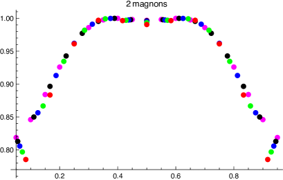
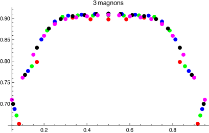
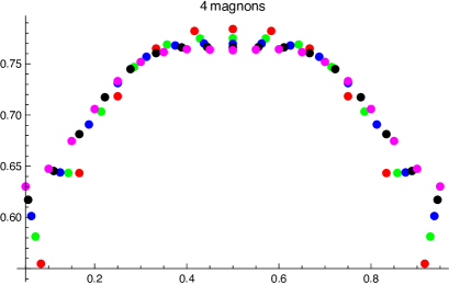
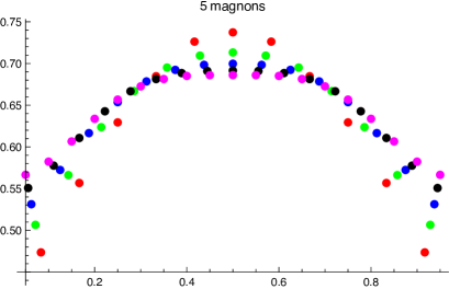
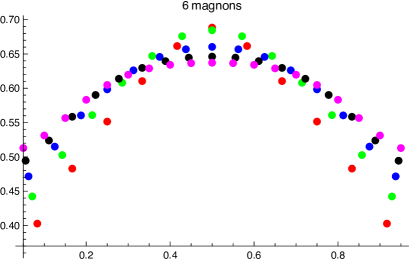
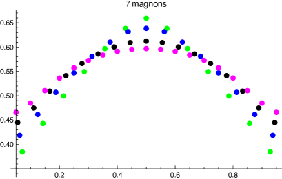
Figure 9: In this figure we present the normalised EE for different number of magnons when the length of the spin chain changes from $L=12$ to $L=20$. The correspondence between colour and length of the spin chain is the following: Red $\Rightarrow$ $L=12$, Green $\Rightarrow$ $L=14$, Blue $\Rightarrow$ $L=16$, Black $\Rightarrow$ $L=18$ & Magenta $\Rightarrow$ $L=20$.

Until now we kept constant the length of the spin chain, modifying the number of the magnons. In figure 9 we change this perspective, keeping constant the number of the magnons while changing the length of the spin chain. As can be seen from all the plots of figure 9, where we present the normalised EE (this is the only quantity that make sense to compare) for different number of magnons (from two to seven) when the length of the spin chain changes, we observe the following pattern. When the number of the magnons is small (from two to four) the curve almost does not change as we change the length of the spin chain. Increasing the number of the magnons, we notice two effects depending on the length of the part of the spin chain we cut: When the length of the cut piece is small the EE increases when we increase the length of the spin chain, while the opposite happens for the EE when the cut piece is close to the half of the spin chain.

In figures 10 and 11 we complete the computation of the EE for the three rank one sectors of ${\cal N}=4$ SYM by repeating the calculation for the $SL(2)$ and the $SU(1|1)$ sectors, respectively. In order to numerically perform these computations we use the same MATHEMATICA code as for the $SU(2)$ sector only changing accordingly the definitions for the functions $f$, $g$, $a$ & $d$, as they appear in equations (A.61) & (A.63), as well as the corresponding scattering matrices for the calculation of the Bethe roots.

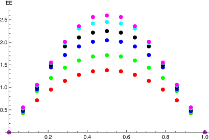
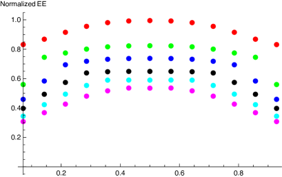
Figure 10: In this figure we repeat the calculations that we presented in figure 8, but for an excited state in the $SL(2)$ sector. The Bethe roots are sitting in two cuts on the real axis. The correspondence between colour and number of magnons is the following: Red $\Rightarrow$ 2 magnons, Green $\Rightarrow$ 3 magnons, Blue $\Rightarrow$ 4 magnons, Black $\Rightarrow$ 5 magnons, Cyan $\Rightarrow$ 6 magnons & Magenta $\Rightarrow$ 7 magnons.

The results for the EE of the $SL(2)$ sector are similar to the ones of the $SU(2)$ sector. We should mention that we have chosen the excited states for which the Bethe roots are sitting in two symmetric cuts on the real axis. In the plots of the normalised EE there are though some differences. Notice that the EE for two magnons almost saturates the bound in the middle of the spin chain and not in some other points as in the $SU(2)$ case. Also the maximum of the curve of the normalised EE is in the middle of the spin chain until we have five magnons, but as we increase their number this maximum is not in the middle any more. This is the inverse picture with respect to the observations of the $SU(2)$ sector, for the normalised EE.

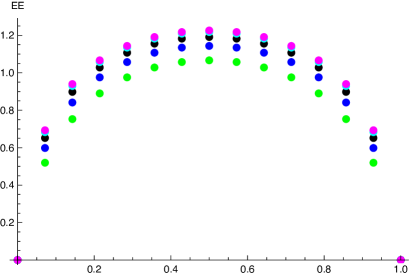
Figure 11: In this figure we repeat the calculations that we presented in figure 8, but for an excited state in the $SU(1|1)$ sector. The correspondence between colour and number of magnons is the following: Green $\Rightarrow$ 3 magnons, Blue $\Rightarrow$ 4 magnons, Black $\Rightarrow$ 5 magnons, Cyan $\Rightarrow$ 6 magnons & Magenta $\Rightarrow$ 7 magnons.

The EE of the of the $SU(1|1)$ sector has some differences with respect to the other two, namely of the $SU(2)$ & $SL(2)$. This is reflected in the right plot of figure 11, where for more than three magnons (the case with two magnons and its particularity has been analysed explicitly at the end of section 2) the pattern we observe is different from the other two sectors. Here the maximum of the normalised EE is when we cut the shortest possible piece of the spin chain, while the minimum is always when we cut the spin chain in the middle. In agreement with the observation in the other two sectors, increasing the number of magnons decreases the normalised EE.

Closing this section we should mention that the two features that remain universal, that is independent of the particular excited state we consider, are the following:

• The fact that the EE per magnon decreases as we increase the number of the magnons.

• For the bosonic subsectors $SU(2)$ & $SL(2)$ the behaviour of the EE presented in figures 8, 9 and 10 is universal, as long as one remains within the broad class of two cut solutions. These solutions are of special interest for the thermodynamic limit and the AdS/CFT correspondence.

5 Conclusions and future directions

The aim of this paper was to exploit integrability in order to shed some light to the behaviour of the Entanglement and Renyi Entropies of the ${\cal N}=4$ SYM spin chain. Generically, the Entanglement and Renyi Entropies depend on the lengths of the spin chain and of the domain of it that we cut, as well as on the details of the excited state whose entropy we are after. These details are the number of propagating magnons, their rapidities and the particular sector on which we focus. Furthermore, since the dilatation operator of ${\cal N}=4$ receives quantum corrections its eigenstates and the associated with them Entanglement and Renyi Entropies will depend on the ’t Hooft coupling $\lambda$. Our goal was to address these questions about how the EE depends on the aforementioned parameters.

After providing the reader with the results for the EE of the vacuum and the single magnon state we analytically calculated the EE of excited states with two magnons in all closed rank one subsectors of ${\cal N}=4$ SYM, namely $SU(2)$, $SU(1|1)$ and $SL(2)$. Our calculation was performed using the formalism of the Coordinate Bethe Ansatz and was leading in the coupling expansion (our states were eigenstates of the one-loop dilatation operators) but exact in the length of the spin chain and of the part of it we cut.

In Section 3 we calculated the EE of the superconformal primary operator with two excitations in the BMN limit. We derived an analytic expression for the EE which is exact in the coupling $\lambda^{\prime}=\frac{g_{YM}^{2}N}{J^{2}}=\frac{\lambda}{J^{2}}$ and interpolates between the weak $\lambda^{\prime}=0$ and strong coupling regimes $\lambda^{\prime}\rightarrow\infty$. This allowed us to analyse the effect of long-range interactions of the spin chain on the EE. We have found that the EE of a part of the spin chain is a monotonically increasing function of the coupling which saturates to a constant value as $\lambda^{\prime}\rightarrow\infty$ when we keep the length of the chain we cut fixed. This results to a violation of a certain bound for the EE that is present at weak coupling. Thus, one of our main conclusions is that, as it is physically anticipated, the entanglement between parts of the chain becomes stronger as one increases the coupling $\lambda^{\prime}$, at least for the superconformal primary operator with two excitations.

In Section 4 we employed integrability, and more precisely the powerful formalism of the Algebraic Bethe Ansatz in order to calculate numerically the EE of excited states with up to seven magnons in the $SU(2)$, $SU(1|1)$ and $SL(2)$ subsectors. In the $SU(2)$ and $SL(2)$ subsectors we have focused on excited state corresponding to 2-cut solutions of the Bethe equations. Although the absolute value of the EE increases with the number of magnons, its normalised value, that is the EE for an $M$ magnon excited state divided by $M$ times the EE of one magnon, decreases with the the number of magnons. Some differences in the behaviour of the EE as a function of the magnon number for the two bosonic sectors are scrutinised in Section 4. The different statistics of the excited states in the $SU(1|1)$ sector lead to a different qualitative behaviour of the normalised EE. This is the only sector that the normalised EE explicitly saturates the bound for the case of two magnons.

A number of very interesting questions remain to be answered. First of all from the perspective of the AdS/CFT correspondence it is important if the calculation of Section 4 for the $SU(2)$ and $SL(2)$ sectors could be performed for a larger number of magnons in longer spin chains. This would allow one to approach the thermodynamic limit in which case the spin chain states will be dual to certain semi-classical string solutions. However, it seems that for this to be achieved a reformulation of the problem will be needed. In particular one should need to obtain expressions for the product of two off-shell states in the thermodynamic limit. One can then address the question of what is the precise relation between the entropy calculated from the spin chain approach and the one which one may calculate from the dual solutions of the non-linear $\sigma$–model . The same question can be asked about the exact in $\lambda^{\prime}$ EE which we have calculated in Section 3. Furthermore, it would be interesting to generalise the calculation of Section 3 to the case of superconformal primary operators with more than two excitations. Another direction would be to calculate the $\frac{1}{J}$ corrections to the BMN EE by considering the near BMN limit.

One could also employ the Perturbative Bethe Ansatz technique to calculate the $g_{YM}^{2}N$ corrections to the EE, as an order by order expansion in perturbation theory. One should of course interpret the fact that eigenstates of the dilatation operators (and as a consequence the corresponding EE) will be scheme-dependent. Notice that such a complication is absent both in the BMN limit considered in Section 3 and in the leading in $g_{YM}^{2}N$ calculations of Section 4.

Appendix A Algebraic Bethe Ansatz: Essential formulas

In this appendix we collect all the essential mathematical formulas needed for the construction of the ABA, following the references Escobedo:2010xs ; Caetano:2011eb ; Escobedo:2012ama . We introduce the following functions that determine the rank one subsector of the ${\cal N}=4$ SYM we are working.

$SU(2)$ sector

The expressions for the basic building blocks are

$$f(u)\equiv 1\,+\,\frac{i}{u}\,,\quad g(u)\equiv\frac{i}{u}\,,\quad h(u)\equiv\frac{f(u)}{g(u)}=\frac{u+i}{i}\,,\quad t(u)\equiv\frac{g(u)^{2}}{f(u)}=\frac{-1}{u(u+i)}\,,$$ (A.58)

$$a(u)\,\equiv\,\left(u\,+\,\frac{i}{2}\right)^{L}\,,\quad d(u)\,\equiv\,\left(u\,-\,\frac{i}{2}\right)^{L},$$ (A.59)

while the $SU(2)$ Bethe equations that determine the set of rapidities, are

$$1\,\equiv\,\left(\frac{u_{j}\,+\,i/2}{u_{j}\,-\,i/2}\right)^{L}\prod_{k\neq j}^{M}\frac{u_{j}\,-\,u_{k}\,-\,i}{u_{j}\,-\,u_{k}\,+\,i}\,.$$ (A.60)

$SL(2)$ sector

The expressions for the basic building blocks are

$$f(u)\,=\,1\,+\,\frac{i}{u}\,,\quad g(u)\,=\,\frac{i}{u}\,,\quad a(u)\,=\,\left(u\,-\,\frac{i}{2}\right)^{L}\,,\quad d(u)\,=\,\left(u\,+\,\frac{i}{2}\right)^{L},$$ (A.61)

while the $SL(2)$ Bethe equations are

$$1\,\equiv\,\left(\frac{u_{j}\,+\,i/2}{u_{j}\,-\,i/2}\right)^{L}\prod_{k\neq j}^{M}\frac{u_{j}\,-\,u_{k}\,+\,i}{u_{j}\,-\,u_{k}\,-\,i}\,.$$ (A.62)

$SU(1|1)$ sector

The expressions for the basic building blocks are

$$f(u)\,=\,\frac{i}{u}\,,\quad g(u)\,=\,\frac{i}{u}\,,\quad a(u)\,=\,\left(u\,+\,\frac{i}{2}\right)^{L}\,,\quad d(u)\,=\,\left(u\,-\,\frac{i}{2}\right)^{L},$$ (A.63)

while the $SU(1|1)$ Bethe equations are

$$1\,\equiv\,\left(\frac{u_{j}\,+\,i/2}{u_{j}\,-\,i/2}\right)^{L}\,.$$ (A.64)

In order to simplify the expressions we introduce the following shorthand notation

$$F^{a}\,\equiv\,\prod_{u_{j}\in\,a}F(u_{j})\,,\qquad F^{a\bar{a}}\,\equiv\!\!\!\prod_{\scriptsize\begin{array}[]{c}{u_{i}}\in a\\ v_{j}\in\bar{a}\end{array}}\!\!\!F(u_{i}-v_{j})\,,\qquad F_{<}^{aa}\,\equiv\!\!\!\prod_{\scriptsize\begin{array}[]{c}{u_{i},u_{j}}\in a\\ i<j\end{array}}\!\!\!F(u_{i}-u_{j})\,.$$ (A.65)

Now we can write the expression for the function $H(a,\bar{a})$, that weights the different partitions of the spin chain, according to the algebraic normalizations of Escobedo:2010xs

$$H(a,\bar{a})\,=\,f^{a\bar{a}}\,d_{r}^{a}\,a_{l}^{\bar{a}}\,,$$ (A.66)

where $a_{l}$ and $d_{r}$ are defined as in equations (A.58), (A.61) & (A.63), but using instead of $L$ the lengths for the left and the right subchain respectively.

Scalar Product

In order to compute the RDM we need to evaluate the scalar product between two Bethe wavefunctions for arbitrary $\{u\}$ and $\{v\}$. A recursion relation for such an expression is computed analytically in references Escobedo:2010xs and Caetano:2011eb . Here, for completeness, we present the outcome of that computation.

Consider two Bethe states, which are parametrized by $u_{i}$ and $v_{i}$, with $i=1,\dots,N$. The scalar product $S_{N}(\{v\},\{u\})\equiv\langle\{v^{*}\}|\{u\}\rangle$ is given by the following recursion relation

$$S_{N}\left(\{v_{1},\dots,v_{N}\},\{u_{1},\dots,u_{N}\}\right)=\sum_{n}b_{n}\,S_{N-1}\left(\{v_{1},\dots,\hat{v}_{n},\dots,v_{N}\},\{\hat{u}_{1},u_{2},\dots,u_{N}\}\right)$$

$$\qquad\qquad-\sum_{n<m}c_{n,m}\,S_{N-1}\left(\{u_{1},v_{1},\dots\hat{v}_{n},\dots,\hat{v}_{m},\dots v_{N}\},\{\hat{u}_{1},u_{2},\dots,u_{N}\}\right)\,,$$ (A.67)

where a Bethe root with a hat means that it is omitted. The definitions for $b_{n}$ and $c_{n,m}$ are the following

$$b_{n}\,=\,g(u_{1}-v_{n})a(v_{n})d(u_{1})\prod_{j\neq n}^{N}\,f(u_{1}-v_{j})\,f(v_{j}-v_{n})\,+\,\left(u_{1}\leftrightarrow v_{n}\right)\,,$$ (A.68)

$$c_{n,m}\,=\,{g(u_{1}-v_{n})\,g(u_{1}-v_{m})\,a(v_{m})\,d(v_{n})}\,{f(v_{n}-v_{m})}\prod_{j\neq n,m}^{N}f(v_{n}-v_{j})\,f(v_{j}-v_{m})\,+\,\left(n\leftrightarrow m\right).$$ (A.69)

Using (A) and substituting the corresponding expressions for the functions $f(u),g(u),a(u)$ and $d(u)$ (from either (A.58), (A.61) or (A.63)), it is possible to calculate the scalar product for any of the rank one subsectrors.

Appendix B Bethe Roots

In section 4 we calculate the EE of excited states that belong either on the $SU(2)$ or on the $SL(2)$ or on the $SU(1|1)$ sector. In this appendix we list the Bethe roots of these excited states and in the $SU(2)$ case we also plot them, since they distribute themselves along two disjoint cuts on the complex plane.

We start from the Bethe roots of the excited states of figures 8 and 9. In those figures we are considering spin chains with 12, 14, 16, 18 & 20 sites with a number of magnons ranging from $2$ to $7$. The Bethe roots for these magnons are the following

$SU(2)$ sector: L=12
2 m $\Rightarrow$ {-1.703, 1.703},
3 m $\Rightarrow$ {-0.478 + 0.500 I, -0.478 - 0.500 I, 1.418}
4 m $\Rightarrow$ {-1.296 + 0.564 I, -1.296 - 0.564 I, 1.296 - 0.564 I, 1.296 + 0.564 I}
5 m $\Rightarrow$ {-1.11 + 0.537 I, -1.11 - 0.537 I, 0.979 - I, 1.009, 0.979 + I}
6 m $\Rightarrow$ {-0.676 + I, -0.676, -0.676 - I, 0.676 - I, 0.676, 0.676 + I}

$SU(2)$ sector: L=14
2 m $\Rightarrow$ {-2.029, 2.029},
3 m $\Rightarrow$ {-0.713 + 0.501 I, -0.713 - 0.501 I, 1.754}
4 m $\Rightarrow$ {-1.644 + 0.601 I, -1.644 - 0.601 I, 1.644 - 0.601 I, 1.644 + 0.601 I}
5 m $\Rightarrow$ {-1.47 + 0.574 I, -1.47 - 0.574 I, 1.428, 1.37 - 1.043 I, 1.37 + 1.043 I}
6 m $\Rightarrow$ {-1.16 + 1.01 I, -1.2, -1.16 - 1.01 I, 1.16 - 1.01 I, 1.2, 1.16 + 1.01 I}
7 m $\Rightarrow$ {-0.898 + 0.994 I, -0.898 - 0.994 I, 0.686 + 1.499 I, 0.686 - 1.499 I,
0.665 - 0.5 I, 0.665 + 0.5 I, -0.907}

$SU(2)$ sector: L=16
2 m $\Rightarrow$ {-2.352, 2.352},
3 m $\Rightarrow$ {-0.922 + 0.502 I, -0.922 - 0.502 I, 2.083}
4 m $\Rightarrow$ {-1.981 + 0.639 I, -1.981 - 0.639 I, 1.981 - 0.639 I, 1.981 + 0.639 I}
5 m $\Rightarrow$ {-1.815 + 0.612 I, -1.815 - 0.612 I, 1.721 - 1.1 I, 1.804, 1.721 + 1.1 I}
6 m $\Rightarrow$ {-1.54 + 1.06 I, -1.6, -1.54 - 1.06 I, 1.54 - 1.06 I, 1.6, 1.54 + 1.06 I}
7 m $\Rightarrow$ {-1.351 + 1.023 I, -1.396, -1.351 - 1.023 I, 1.230 - 1.464 I,
1.262 - 0.502 I, 1.262 + 0.502 I, 1.23 + 1.464 I}

$SU(2)$ sector: L=18
2 m $\Rightarrow$ {-2.675, 2.675},
3 m $\Rightarrow$ {-1.117 + 0.505 I, -1.117 - 0.505 I, 2.408}
4 m $\Rightarrow$ {-2.312 + 0.675 I, -2.312 - 0.675 I, 2.312 - 0.675 I, 2.312 + 0.675 I}
5 m $\Rightarrow$ {-2.15 + 0.65 I, -2.15 - 0.65 I, 2.063 - 1.156 I, 2.159, 2.063 + 1.156 I}
6 m $\Rightarrow$ {-1.89 + 1.1 I, -1.98, -1.89 - 1.1 I, 1.89 - 1.1 I, 1.98, 1.89 + 1.1 I}
7 m $\Rightarrow$ {1.614 - 1.503 I, 1.702 - 0.511 I, 1.702 + 0.511 I, 1.614 + 1.503 I,
-1.719 + 1.074 I, -1.790, -1.719 - 1.074 I}

$SU(2)$ sector: L=20
2 m $\Rightarrow$ {-2.996, 2.996},
3 m $\Rightarrow$ {-1.302 + 0.51 I, -1.302 - 0.51 I, 2.732}
4 m $\Rightarrow$ {-2.64 + 0.71 I, -2.64 - 0.71 I, 2.64 - 0.71 I, 2.64 + 0.71 I}
5 m $\Rightarrow$ {-2.48 + 0.685 I, -2.48 - 0.685 I, 2.397 - 1.214 I, 2.5, 2.397 + 1.214 I}
6 m $\Rightarrow$ {-2.23 + 1.17 I, -2.3, -2.23 - 1.17 I, 2.23 - 1.17 I, 2.3, 2.23 + 1.17 I}
7 m $\Rightarrow$ {1.965 - 1.567 I, 2.090 - 0.525 I, 2.090 + 0.525 I, 1.965 + 1.567 I,
-2.066 + 1.131 I, -2.153, -2.066 - 1.131 I}

We only plot the Bethe roots that correspond to a spin chain with 14 sites, since all the other plots are similar.

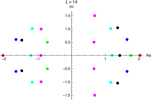
Figure 12: The correspondence between colour and number of magnons is the following: Red $\Rightarrow$ 2 magnons, Green $\Rightarrow$ 3 magnons, Blue $\Rightarrow$ 4 magnons, Black $\Rightarrow$ 5 magnons, Cyan $\Rightarrow$ 6 magnons & Magenta $\Rightarrow$ 7 magnons.

The Bethe roots that correspond to the excited states of the figures 10 ($SL(2)$ sector) and 11 ($SU(1|1)$ sector), for a spin chain with with $14$ sites, are the following

$SL(2)$ sector
2 m $\Rightarrow$ {-2.352, 2.352},
3 m $\Rightarrow$ {-1.889, -3.069, 2.521}
4 m $\Rightarrow$ {-2.024, -3.268, 3.268, 2.024}
5 m $\Rightarrow$ {-2.166, -3.472, 3.946, 2.652, 1.726}
6 m $\Rightarrow$ {-1.845, 1.845, -2.822, -4.17, 4.17, 2.822}
7 m $\Rightarrow$ {4.831, 1.619, 2.415, 3.437, -1.97, -2.998, -4.398}

and

$SU(1|1)$ sector
3 m $\Rightarrow$ {0.399, 0.627, 1.038}
4 m $\Rightarrow$ {0, 0.114, 0.241, 0.399, 0.627}
5 m $\Rightarrow$ {-2.166, -3.472, 3.946, 2.652, 1.726}
6 m $\Rightarrow$ {-0.175, -0.056, 0.056, 0.175, 0.314, 0.5}
7 m $\Rightarrow$ {-0.399, -0.241, -0.114, 0, 0.114, 0.241, 0.399}

References

- (1) C. Holzhey, F. Larsen and F. Wilczek, “Geometric and renormalized entropy in conformal field theory,” Nucl. Phys. B 424, 443 (1994) [hep-th/9403108].
- (2) P. Calabrese and J. L. Cardy, “Entanglement entropy and quantum field theory,” J. Stat. Mech. 0406, P06002 (2004) [hep-th/0405152].
- (3) S. Ryu and T. Takayanagi, “Holographic derivation of entanglement entropy from AdS/CFT,” Phys. Rev. Lett. 96, 181602 (2006) [hep-th/0603001].
- (4) S. Ryu and T. Takayanagi, “Aspects of Holographic Entanglement Entropy,” JHEP 0608, 045 (2006) [hep-th/0605073].
- (5) H. Casini, M. Huerta and R. C. Myers, “Towards a derivation of holographic entanglement entropy,” JHEP 1105, 036 (2011) [arXiv:1102.0440 [hep-th]].
- (6) A. Lewkowycz and J. Maldacena, “Generalized gravitational entropy,” JHEP 1308, 090 (2013) [arXiv:1304.4926 [hep-th]].
- (7) I. R. Klebanov, D. Kutasov and A. Murugan, “Entanglement as a probe of confinement,” Nucl. Phys. B 796, 274 (2008) [arXiv:0709.2140 [hep-th]].
- (8) G. Georgiou and D. Zoakos, “Entanglement entropy of the Klebanov-Strassler model with dynamical flavors,” JHEP 1507, 003 (2015) [arXiv:1505.01453 [hep-th]].
- (9) V. Alba, M. Fagotti and P. Calabrese, “Entanglement entropy of excited states,” J. Stat. Mech. 0910, P10020 (2009) [arXiv:0909.1999 [cond-mat.stat-mech]].
- (10) J. I. Latorre and A. Riera, “A short review on entanglement in quantum spin systems,” J. Phys. A 42, 504002 (2009) [arXiv:0906.1499 [cond-mat.stat-mech]].
- (11) N. Beisert et al., “Review of AdS/CFT Integrability: An Overview,” Lett. Math. Phys. 99, 3 (2012) [arXiv:1012.3982 [hep-th]].
- (12) J. M. Maldacena, “The Large N limit of superconformal field theories and supergravity,” Int. J. Theor. Phys. 38, 1113 (1999) [Adv. Theor. Math. Phys. 2, 231 (1998)] [hep-th/9711200].
- (13) A. V. Ramallo, “Introduction to the AdS/CFT correspondence,” Springer Proc. Phys. 161, 411 (2015) [arXiv:1310.4319 [hep-th]].
- (14) J. D. Edelstein, J. P. Shock and D. Zoakos, “The AdS/CFT Correspondence and Non-perturbative QCD,” AIP Conf. Proc. 1116, 265 (2009) [arXiv:0901.2534 [hep-ph]].
- (15) M. Staudacher, “The Factorized S-matrix of CFT/AdS,” JHEP 0505, 054 (2005) [hep-th/0412188].
- (16) J. Mölter, T. Barthel, U. Schollwöck and V. Alba, “Bound states and entanglement in the excited states of quantum spin chains,” J. Stat. Mech. 1410, no. 10, P10029 (2014) [arXiv:1407.0066 [cond-mat.str-el]].
- (17) D. E. Berenstein, J. M. Maldacena and H. S. Nastase, “Strings in flat space and pp waves from N=4 superYang-Mills,” JHEP 0204, 013 (2002) [hep-th/0202021].
- (18) N. Beisert, “The dynamic S-matrix,” Adv. Theor. Math. Phys. 12, 948 (2008) [hep-th/0511082].
- (19) S. Lee and R. Russo, “Holographic cubic vertex in the pp-wave,” Nucl. Phys. B 705, 296 (2005) [hep-th/0409261].
- (20) S. Dobashi and T. Yoneya, “Resolving the holography in the plane-wave limit of AdS/CFT correspondence,” Nucl. Phys. B 711, 3 (2005) [hep-th/0406225].
- (21) C. S. Chu, V. V. Khoze and G. Travaglini, “Three point functions in N=4 Yang-Mills theory and pp waves,” JHEP 0206, 011 (2002) [hep-th/0206005].
- (22) G. Georgiou and V. V. Khoze, “BMN operators with three scalar impurites and the vertex correlator duality in pp wave,” JHEP 0304, 015 (2003) [hep-th/0302064].
- (23) G. Georgiou, V. L. Gili and R. Russo, “Operator mixing and three-point functions in N=4 SYM,” JHEP 0910, 009 (2009) [arXiv:0907.1567 [hep-th]].
- (24) G. Georgiou and G. Travaglini, “Fermion BMN operators, the dilatation operator of N=4 SYM, and pp wave string interactions,” JHEP 0404, 001 (2004) [hep-th/0403188].
- (25) M. S. Costa, R. Monteiro, J. E. Santos and D. Zoakos, “On three-point correlation functions in the gauge/gravity duality,” JHEP 1011, 141 (2010) [arXiv:1008.1070 [hep-th]].
- (26) G. Georgiou, “Two and three-point correlators of operators dual to folded string solutions at strong coupling,” JHEP 1102, 046 (2011) [arXiv:1011.5181 [hep-th]].
- (27) G. Georgiou, “SL(2) sector: weak/strong coupling agreement of three-point correlators,” JHEP 1109, 132 (2011) [arXiv:1107.1850 [hep-th]].
- (28) N. Beisert, “BMN operators and superconformal symmetry,” Nucl. Phys. B 659, 79 (2003) [hep-th/0211032].
- (29) G. Georgiou, V. L. Gili and R. Russo, “Operator Mixing and the AdS/CFT correspondence,” JHEP 0901, 082 (2009) [arXiv:0810.0499 [hep-th]].
- (30) G. Georgiou, V. V. Khoze and G. Travaglini, “New tests of the pp wave correspondence,” JHEP 0310, 049 (2003) [hep-th/0306234].
- (31) G. Georgiou, V. Gili, A. Grossardt and J. Plefka, “Three-point functions in planar N=4 super Yang-Mills Theory for scalar operators up to length five at the one-loop order,” JHEP 1204, 038 (2012) [arXiv:1201.0992 [hep-th]].
- (32) R. C. Myers and A. Sinha, “Seeing a c-theorem with holography,” Phys. Rev. D 82, 046006 (2010) [arXiv:1006.1263 [hep-th]].
- (33) R. C. Myers and A. Sinha, “Holographic c-theorems in arbitrary dimensions,” JHEP 1101, 125 (2011) [arXiv:1011.5819 [hep-th]].
- (34) C. Beck and F. Schlögl, “Thermodynamics of chaotic systems”, (Cambridge University Press, Cambridge, 1993).
- (35) L. D. Faddeev, “How algebraic Bethe ansatz works for integrable model,” hep-th/9605187.
- (36) J. Escobedo, N. Gromov, A. Sever and P. Vieira, “Tailoring Three-Point Functions and Integrability,” JHEP 1109, 028 (2011) [arXiv:1012.2475 [hep-th]].
- (37) T. Bargheer, N. Beisert and N. Gromov, “Quantum Stability for the Heisenberg Ferromagnet,” New J. Phys. 10, 103023 (2008) [arXiv:0804.0324 [hep-th]].
- (38) J. Escobedo, “Integrability in AdS/CFT: Exact Results for Correlation Functions,” Ph.D thesis
- (39) H. Casini and M. Huerta, “Entanglement entropy in free quantum field theory,” J. Phys. A 42, 504007 (2009) [arXiv:0905.2562 [hep-th]].
- (40) J. Caetano and J. Escobedo, “On four-point functions and integrability in N=4 SYM: from weak to strong coupling,” JHEP 1109, 080 (2011) [arXiv:1107.5580 [hep-th]].