The joint distribution of the Parisian ruin time and the number of claims until Parisian ruin in the classical risk model

Abstract

In this paper we propose new iterative algorithm of calculating the joint distribution of the Parisian ruin time and the number of claims until Parisian ruin for the classical risk model. Examples are provided when the generic claim size is exponentially distributed.

Keywords: classical risk model, number of claims, Parisian ruin.

1 Introduction

The distribution of the number of claims until ruin has been in the centre of interest for many years. One of the first references dealing with this problem is Beard [1]. The main first step was done by Stanford and Stroiński [17] who produced recursive procedures to calculate the probability of ruin at the $n$th claim arrival epoch in the classical risk model. Egído dos Reis [7] derived the moment generating function of the number of claims until ruin in the classical risk model. He inverted this for certain claim size distributions, and, using a duality argument, found moments of the number of claims until ruin when the initial surplus is $0$. The next main step was done by Landriault et al. [13] who considered a Sparre Andersen risk model with exponential claims. Using Gerber-Shiu type analysis (see Gerber and Shiu [9])) they derived a number of results including an expression for the probability function of the number of claims until ruin. The main idea of getting these nice results followed approach of Dickson and Willmot [6]. The main results of our paper are closely related with the seminal paper of Dickson [5] who using probabilistic arguments derived the expression for the joint density of the time of ruin and the number of claims until ruin in the classical risk model. From this he obtained a general expression for the probability function of the number of claims until ruin. He also considered the moments of the number of claims until ruin and illustrate all results in the case of exponentially distributed individual claims. Frostig et al.[8] and Zhao and Zhang [18] analyzed similar problems.

In this paper we extend results concerning classical ruin into so-called Parisian type of ruin. This type of ruin occurs if the surplus process falls below zero and stays below zero for a continuous time of interval of length $d$; see Figure 1. We believe that the Parisian ruin probability and other related quantities might be more appropriate measures of risk than the ones identified for the classical ruin. The main reason is that it gives the insurance companies the chance to achieve solvency. The idea of Parisian ruin comes from Parisian options which was first introduced by Chesney et al. [2]. Dassios and Wu [4] considered the Parisian ruin probability for the classical risk model with exponential claims and for the Brownian motion with drift. Czarna and Palmowski [3] and Loeffen et al. [15] analyzed the Parisian ruin probability for a general spectrally negative Lévy process. Other relevant papers are Landriault et al. [11] and [12], where the deterministic and fix delay $d$ is replaced by an independent exponential random variable.

Our paper in a sense has similar goal like in Dickson [5] and Landriault et al. [11], that is we want to identify the joint density of the time of Parisian ruin and the number of claims until Parisian ruin. Although our focus is more consistent with Stanford and Stroiński [17] - we want to create efficient iterative algorithm of finding above quantity.

Formally, in this paper we consider a continuous-time surplus process:

$$U(t):=u+ct-\sum_{i=1}^{N_{t}}X_{i},$$ (1)

where the non-negative constant $u$ denotes the initial reserve, the positive constant $c$ is the rate of premium income, $N_{t}$ describes the number of claims counted up to time $t$ which is a Poisson process with parameter $\lambda$ and $\{X_{i}\}_{i=1}^{\infty}$ are claim sizes which are independent and identically distributed non-negative random variables that are also independent of $N_{t}$. We denote by $F(x)$ and $f(x)$ the distribution function and density function, respectively. We assume $c>\lambda\mathbb{E}(X_{1})$ assuring that ruin is not certain.

We define the Parisian time of ruin by

$$\tau_{u}^{d}:=\inf\{t>0:t-\sup\{s<t:U(s)\geq 0\}\geq d,U(t)<0\}.$$

We denote the joint density of $N_{\tau_{u}^{d}}$ and $\tau_{u}^{d}$ by (hereafter $\mathbb{N}=\{0,1,2,\cdots\}$):

$$w_{u}^{d}(n,t):=\frac{d}{dt}\psi_{u}^{d}(n,t),\ \ \ n\in\mathbb{N},t\geq 0$$

with

$$\psi_{u}^{d}(n,t):=\mathbb{P}(N_{\tau_{u}^{d}}=n,\tau_{u}^{d}\leq t|U(0)=u),\ \ \ n\in\mathbb{N},t\geq d.$$ (2)

Further, let $p_{u}^{d}(n)$ denotes the probability that there have been exactly $n$ claims up to Parisian ruin event, so that

$$p_{u}^{d}(n) := \mathbb{P}(N_{\tau_{u}^{d}}=n,\tau_{u}^{d}<\infty|U(0)=u)=\int_{d}^{\infty}w_{u}^{d}(n,t)dt.$$ (3)

The main goal of this paper is to give efficient iterative algorithm of calculating of $w_{u}^{d}(n,t)$ and hence $p_{u}^{d}(n)$.

Note that the $d=0$ case corresponds to the classical ruin problem. Then we deal with the classical ruin time of the risk process (1):

$$\tau_{u}:=\inf\{t\geq 0:U(t)<0\}.$$ (4)

The rest of the paper is organized as follows. In Section 2 we give the main representations of the joint density of $N_{\tau^{d}}$ and $\tau^{d}$ and prove the main results. Finally, in Section 3 we analyze some particular examples and give extensive numerical analysis.

2 Main representation

Since Parisian ruin occurs if the surplus falls below zero and stays below zero for a continuous time interval of length $d$, Parisian ruin time must be larger than $d$. Throughout this paper, we can assume that $w_{u}^{d}(n,t)=0$ when $t\leq d,u\geq 0$. For $t>d$ and $u\geq 0$ we will now identify the joint density $w_{u}^{d}(n,t)$ ($n\in\mathbb{N}$) of $N_{\tau_{u}^{d}}$ and $\tau_{u}^{d}$.

2.1 The expression of the joint density $w_{u}(k,t,y)$

Our results heavily use the main result of Dickson [5]. He considers the joint density of the number $N_{\tau_{u}}$ of claims until ruin (including the ruin-caused claim), $\tau_{u}$ given in (4) and the deficit at ruin $|U(\tau_{u})|$ defined by :

$$w_{u}(k,t,y):=\frac{\partial^{2}}{\partial t\partial y}\psi_{u}(k,t,y),\ \ \ k\in\mathbb{N},t\geq 0,y>0$$

with

$$\psi_{u}(k,t,y):=\mathbb{P}(N_{\tau_{u}}=k,\tau_{u}\leq t,|U(\tau_{u})|\leq y\big{|}U(0)=u),\ \ \ k\in\mathbb{N},t\geq 0,y>0.$$

For any function $g$ we denote by $g^{k*}$ ($k\geq 0$) the $k$-fold convolution of $g$ with itself, where $g^{1*}=g$ and $g^{0*}(t)=\delta_{0}(t)$ for the impulse function $\delta_{0}$ at $0$. We are now in position to state the main result of Dickson [5].

Theorem 2.1

For $k=1,2,\ldots$ we have that

$$w_{0}(k,t,y) = \int_{0}^{ct}\frac{x}{ct}e^{-\lambda t}\frac{\lambda^{k}t^{k-1}}{(k-1)!}f^{(k-1)*}(ct-x)f(x+y)dx$$ (5)

and for $u>0$

$$w_{u}(k,t,y) = \int_{0}^{u+ct}e^{-\lambda t}\frac{\lambda^{k}t^{k-1}}{(k-1)!}f^{(k-1)*}(u+ct-x)f(x+y)dx$$

$$-c\sum_{j=1}^{k-1}\int_{0}^{t}e^{-\lambda s}\frac{(\lambda s)^{j}}{j!}f^{j*}(u+cs)\omega_{0}(k-j,t-s,y)ds.$$

Corollary 2.2

When the generic claim amount is exponentially distributed with mean $1/\mu$, i.e. $f(x)=\mu e^{-\mu x}$, then

$$w_{0}{(k,t,y)}=\frac{\lambda^{k}\mu^{k}c^{k-1}}{k!(k-1)!}t^{2k-2}e^{-(\lambda+\mu c)t}e^{-\mu y},$$ (6)

$$w_{u}{(k,t,y)}=\frac{\lambda^{k}\mu^{k}(ku+ct)(u+ct)^{k-2}}{k!(k-1)!}t^{k-1}e^{-(\lambda+\mu c)t-\mu u}e^{-\mu y}.$$ (7)

For $u\geq 0$ we denote by the density of having $k$ claims up to the classical ruin time $\tau_{u}$ and having the deficit $y$ at the ruin:

$$w_{u}(k,y) = \int_{0}^{\infty}w_{u}(k,t,y)dt.$$

In particular, for exponential claim size with intensity $\mu$ we have:

$$w_{0}(k,y)=\frac{(2k-2)!}{k!(k-1)!}\frac{\lambda^{k}\mu^{k}c^{k-1}}{(\lambda+\mu c)^{2k-1}}e^{-\mu y}.$$

2.2 The joint distribution of the first upward passage time and the number of claims

For $y\geq 0$ we define the first upward passage time of our classical risk process:

$$\tau_{y}^{+}=\min\{s\geq 0,U(s)=y|U(0)=0\}.$$

We denote by

$$v_{y}(k,t):=\frac{d}{dt}V_{y}(k,t),\ \ \ k\in\mathbb{N},t\geq y/c$$

the density of having $k$ jumps up to first passage time of level $y$ that happens at time $t$, that is:

$$V_{y}(k,t):=\mathbb{P}(N_{\tau_{y}^{+}}=k,\tau_{y}^{+}\leq t|U(0)=0),\ \ \ k\in\mathbb{N},t\geq 0.$$

Theorem 2.3

We have:

$$v_{y}(k,t) = \frac{\lambda^{k}}{k!}yt^{k-1}e^{-\lambda t}f^{k*}(ct-y).$$ (9)

Proof. For $r\in(0,1]$ and $\delta>0$, we define the bivariate Laplace transform of $(\tau_{y}^{+},N_{\tau_{y}^{+}})$:

$$\phi(y) := E[r^{N_{\tau_{y}^{+}}}e^{-\delta\tau_{y}^{+}}\mathbb{I}(\tau_{y}^{+}<\infty)|U(0)=0]$$ (10)

$$= \int_{0}^{\infty}e^{-\delta t}\sum_{k=0}^{\infty}r^{k}v_{y}(k,t)dt.$$

Considering an infinitesimal time interval $(0,dt)$ we have:

$$\phi(y) = e^{-\delta dt}e^{-\lambda dt}\phi(y-cdt)+re^{-\delta dt}(1-e^{-\lambda dt})\int_{0}^{\infty}\phi(y-cdt+x)f(x)dx+o(dt)$$ (11)

$$= [1-(\lambda+\delta)dt]\phi(y-cdt)+\lambda rdt\int_{0}^{\infty}\phi(y-cdt+x)f(x)dx+o(dt).$$

Subtracting $\phi(y-ct)$ from both sides of above equation, multiplying by $1/dt$ and letting $dt\rightarrow 0$ produce the following integro-differential equation:

$$c\phi^{{}^{\prime}}(y)=-(\lambda+\delta)\phi(y)+\lambda r\int_{0}^{\infty}\phi(y+x)f(x)dx.$$ (12)

Clearly, when $y=0$, we have

$$\phi(0)=1.$$ (13)

Since the solution to (12) with boundary condition (13) is unique, we assume that $\phi(y)$ is of the form

$$\phi(y)=c(y)e^{-by}.$$

The boundary condition $\phi(0)=1$ gives $c(y)=1$, so that $\phi(y)=e^{-by}$. Note that the real part of $b$ must be positive, because otherwise it would be a contradiction to the fact that $\lim_{y\rightarrow\infty}\phi(y)=0$. It is known that the Lundberg’s fundamental equation of the classical risk model is given by

$$\lambda+\delta-cs=\lambda r\hat{f}(s).$$

We denote the positive solution by $\rho$.

Now, using a similar approach as in Li [14], Zhao and Zhang [18] we can obtain the solution of the integro-differential equation (12):

$$\phi(y)=e^{-\rho y}.$$

We recall now the Lagrange’s Expansion Theorem (see Lagrange [10, p. 251-326]). Given two functions $\alpha(z)$ and $\beta(z)$ which are both analytic on and inside a contour $D$ surrounding a point $a$, if $r$ satisfies the inequality

$$|r\beta(z)|<|z-a|,$$ (14)

for every $z$ on the perimeter of $D$, then $z-a-r\varphi(z)$, as a function of $z$, has exactly one zero $\eta$ in the interior of $D$, and we have further

$$\alpha(\eta)=\alpha(a)+\sum_{k=1}^{\infty}\frac{r^{k}}{k!}\frac{d^{k-1}}{dx^{k-1}}\big{(}\alpha^{\prime}(x)\beta^{k}(x)\big{)}\!\big{|}_{x=a}.$$ (15)

It follows from above fact that:

$$e^{-\rho y}=\int_{0}^{\infty}e^{-\delta t}\sum_{k=0}^{\infty}r^{k}\left(\frac{\lambda^{k}}{k!}yt^{k-1}e^{-\lambda t}f^{k*}(ct-y)\right)dt.$$ (16)

Comparing (10) and (16) gives the assertion of the theorem. $\Box$

Corollary 2.4

When the individual claim amounts are exponentially distributed with mean $1/\mu$ then

$$v_{y}(k,t)=\left\{\begin{array}[]{lll}&\frac{y}{t}e^{-\lambda t}\delta_{0}(ct-y),&k=0,\\ &\frac{\lambda^{k}\mu^{k}y}{k!(k-1)!}t^{k-1}(ct-y)^{k-1}e^{-(\lambda+\mu c)t}e^{\mu y},&k>0.\end{array}\right.$$ (19)

2.3 The expression of $w_{u}^{d}(n,t)$

Recall that $w_{u}^{d}(n,t)$ is the joint density that Parisian ruin occurs at time $t$ and there are $n$ claims up to time $t$. The main result of this paper gives recursive algorithm of calculating the density $w_{u}^{d}(k,t)$.

Theorem 2.5

We have

$$w_{u}^{d}(1,t)=\lambda e^{-\lambda t}\bar{F}(u+ct)$$ (20)

and for $n=2,3,\ldots$,

$$w_{u}^{d}(n,t)=$$ (22)

$$= \sum_{k=0}^{n-1}\int_{cd}^{\infty}w_{u}(n-k,t-d,y)\frac{(\lambda d)^{k}}{k!}e^{-\lambda d}dy+\sum_{k=1}^{n-1}\int_{0}^{cd}w_{u}(n-k,t-d,y)$$

$$\times\Big{[}\frac{(\lambda d)^{k}}{k!}e^{-\lambda d}\bar{F}^{k*}(cd-y)-\sum_{m=0}^{k-1}\int_{\frac{y}{c}}^{d}v_{y}(m,s)\frac{(\lambda(d-s))^{k-m}}{(k-m)!}e^{-\lambda(d-s)}\bar{F}^{(k-m)*}(c(d-s))ds\Big{]}dy$$

$$+\sum_{l=1}^{n-1}\sum_{k=0}^{n-l-1}\int_{0}^{cd}\int_{\frac{y}{c}}^{d}\int_{0}^{\max(t-d-s,0)}w_{u}(l,t_{1},y)v_{y}(k,s)w_{0}^{d}(n-l-k,t-t_{1}-s)dt_{1}dsdy.$$

Proof. Fact that the Parisian ruin occurs in the time interval $(0,t]$ and there is only one claim up to Parisian ruin time, means that only one claim occurs before time $t-d$ that cause the classical ruin, the deficit is larger than $cd$ and there will be no claims within time that risk process spent below $0$, see Figure 2. This gives (20).

The arguments behind the formula (22) are as follows. We know that the Parisian ruin occurs after classical ruin. There are only two cases:

• $\tau^{d}_{u}=\tau_{u}+d$, i.e., the surplus will stay below zero for a continuous time interval of length $d$ after the classical ruin time. Let us assume that there are $k$ $(0\leq k\leq n-1)$ claims during the interval $(\tau_{u},\tau_{u}+d]$ and $n-k$ claims during the interval $(0,\tau_{u}]$. If the deficit at the classical ruin is more than $cd$ then the surplus can not exceed $0$ before $\tau_{u}+d$ no matter how much the cumulative amount of the $k$ claims is. This covers the first term of formula (22). However, if the deficit is less than $cd$ (formulated as the second term) then it also includes the possibility that the surplus has been up-crossing $0$ prior to time $\tau_{u}+d$ which should be subtracted. To take into account w suppose that $\tau_{u}+s$ is the first time before $\tau_{u}+d$ at which there was an up-crossing of the surplus process through $0$ and there are $m$ claims during the interval $(\tau_{u},\tau_{u}+s]$ and hence $k-m$ claims during the interval $(\tau_{u}+s,\tau_{u}+d]$.

• $\tau^{d}_{u}>\tau_{u}+d$, i.e., the surplus exceeds $0$ in the interval $(\tau_{u},\tau_{u}+d]$ (we assume also that classical ruin happens at time $t_{1}$). We apply probabilistic arguments to construct the last term of (22); see Prabhu[16]. We take $\tau_{u}+s$ to be the first time before $\tau_{u}+d$ at which there is an up-crossing of the surplus process through $0$. Further, we suppose that there are $l$ claims in $(0,\tau_{u}]$ and $k$ claims in $(\tau_{u},\tau_{u}+s]$. Additionally, when risk process up-crosses zero it does in continuous way. So we can restart the our considerations with $u=0$, the Parisian ruin time equal to $t-t_{1}-s$ and $(n-l-k)$ amount of claims counted up to this time.

$\Box$

In particular, from (22) for $u=0$ we can obtain the following corollary.

Corollary 2.6

$$w_{0}^{d}(n,t)$$ (24)

$$= \sum_{k=0}^{n-1}\int_{cd}^{\infty}w_{0}(n-k,t-d,y)\frac{(\lambda d)^{k}}{k!}e^{-\lambda d}dy+\sum_{k=1}^{n-1}\int_{0}^{cd}w_{0}(n-k,t-d,y)$$

$$\times\Big{[}\frac{(\lambda d)^{k}}{k!}e^{-\lambda d}\bar{F}^{k*}(cd-y)-\sum_{m=0}^{k-1}\int_{\frac{y}{c}}^{d}v_{y}(m,s)\frac{(\lambda(d-s))^{k-m}}{(k-m)!}e^{-\lambda(d-s)}\bar{F}^{(k-m)*}(c(d-s))ds\Big{]}dy$$

$$+\sum_{l=1}^{n-1}\sum_{k=0}^{n-l-1}\int_{0}^{cd}\int_{\frac{y}{c}}^{d}\int_{0}^{\max(t-d-s,0)}w_{0}(l,t_{1},y)v_{y}(k,s)w_{0}^{d}(n-l-k,t-t_{1}-s)dt_{1}dsdy.$$

In order to find the explicit expression of $w_{0}^{d}(n,t)$, we first consider $w_{0}^{d}(1,t)$ which denotes the joint density function when Parisian ruin occurs at time $t$ and there is only one claim up to time $t$. Plugging $u=0$ into (20) we have:

$$w_{0}^{d}(1,t)=\lambda e^{-\lambda t}\bar{F}(ct),\ \ \ \ \ t>d.$$ (25)

Then substituting (25), (9) and (5) into (24), we can get the expression of $w_{0}^{d}(2,t)$. Similarly, using the expressions of $w_{0}^{d}(1,t)$ and $w_{0}^{d}(2,t)$ we can obtain the expression of $w_{0}^{d}(3,t)$. By applying this iterative algorithm we can identify $w_{0}^{d}(n,t)$ for any $n>0$.

Putting the expression of $w_{0}^{d}(n,t)$ into the equation (22) and using the expression of $w_{u}(k,t,y)$ given in Section 2.1 allows to calculate the density $w_{u}^{d}(n,t)$ for any $u>0$. We will show later how this algorithm could be used in some examples.

Remark We denote by $w_{u}^{d}(n,t,x)$ the joint density of the number of claims until Parisian ruin time (the corresponding argument is denoted by $(n)$), the time to Parisian ruin (the corresponding argument is denoted by $(t)$) and the deficit at Parisian ruin (the corresponding argument is denoted by $(x)$). Then similar considerations that gave (22) gives:

$$w_{u}^{d}(n,t,x)$$ (26)

$$=\sum_{k=0}^{n-1}\int_{cd}^{\infty}w_{u}(n-k,t-d,y)\frac{(\lambda d)^{k}}{k!}e^{-\lambda d}f^{k*}(cd-y+x)dy+\sum_{k=1}^{n-1}\int_{0}^{cd}w_{u}(n-k,t-d,y)$$

$$\times\Big{[}\frac{(\lambda d)^{k}}{k!}e^{-\lambda d}f^{k*}(cd-y+x)-\sum_{m=0}^{k-1}\int_{\frac{y}{c}}^{d}v_{y}(m,s)\frac{(\lambda(d-s))^{k-m}}{(k-m)!}e^{-\lambda(d-s)}f^{(k-m)*}(c(d-s)+x)ds\Big{]}dy$$

$$+\sum_{l=1}^{n-1}\sum_{k=0}^{n-l-1}\int_{0}^{cd}\int_{\frac{y}{c}}^{d}\int_{0}^{\max(t-d-s,0)}w_{u}(l,t_{1},y)v_{y}(k,s)w_{0}^{d}(n-l-k,t-t_{1}-s,x)dt_{1}dsdy.$$

There is another interesting observation. Denote the sum of the first term and the second term of formula (24) by

$$h(n,t)$$

$$:= \sum_{k=0}^{n-1}\int_{cd}^{\infty}w_{0}(n-k,t-d,y)\frac{(\lambda d)^{k}}{k!}e^{-\lambda d}dy+\sum_{k=1}^{n-1}\int_{0}^{cd}w_{0}(n-k,t-d,y)$$

$$\times\Big{[}\frac{(\lambda d)^{k}}{k!}e^{-\lambda d}\bar{F}^{k*}(cd-y)-\sum_{m=0}^{k-1}\int_{\frac{y}{c}}^{d}v_{y}(m,s)\frac{(\lambda(d-s))^{k-m}}{(k-m)!}e^{-\lambda(d-s)}\bar{F}^{(k-m)*}(c(d-s))ds\Big{]}dy.$$

Let

$$\varpi(m,z) = \sum_{k=0}^{m-1}\int_{0}^{cd}w_{0}(m-k,z-s,y)\int_{\frac{y}{c}}^{d}v_{y}(k,s)dsdy.$$

Then the equation (24) can be written more concisely as follows:

$$w_{0}^{d}(n,t) = h(n,t)+\sum_{m=1}^{n-1}\int_{0}^{t-d}\varpi(m,z)w_{0}^{d}(n-m,t-z)dz.$$ (30)

In probability theory, (30) is known as a (bivariate) renewal equation for the function $w_{0}^{d}$. It is known that the solution of (30) can be expressed as an infinite series of functions:

$$w_{0}^{d}(n,t) = \sum_{k=0}^{\infty}\Big{(}h*\varpi^{k**}\Big{)}(n,t).$$ (31)

2.4 The expression of $p_{u}^{d}(n)$

In this section we will identify $p_{u}^{d}(n)$ given in (3) describing the probability of having $n$ claims up to Parisian ruin time. Recall that from (3)

$$p_{u}(n)=\int_{d}^{\infty}w_{u}^{d}(n,t)dt.$$

Hence from Theorem 2.5 we have the following result.

Theorem 2.7

$$p_{u}^{d}(1)=\int_{0}^{\infty}\lambda e^{-\lambda t}\bar{F}(u+ct+cd)e^{-\lambda d}dt$$

and for $n=2,3,\ldots,$

$$p_{u}^{d}(n) = \sum_{k=0}^{n-1}\int_{cd}^{\infty}w_{u}(n-k,y)\frac{(\lambda d)^{k}}{k!}e^{-\lambda d}dy+\sum_{k=1}^{n-1}\int_{0}^{cd}w_{u}(n-k,y)$$ (32)

$$\times\Big{[}\frac{(\lambda d)^{k}}{k!}e^{-\lambda d}\bar{F}^{k*}(cd-y)-\sum_{m=0}^{k-1}\int_{\frac{y}{c}}^{d}v_{y}(m,s)\frac{(\lambda(d-s))^{k-m}}{(k-m)!}e^{-\lambda(d-s)}\bar{F}^{(k-m)*}(c(d-s))ds\Big{]}dy$$

$$+\sum_{m=1}^{n-1}\sum_{k=0}^{n-m-1}\int_{0}^{cd}\int_{\frac{y}{c}}^{d}w_{u}(m,y)v_{y}(k,s)p_{0}^{d}(n-m-k)dsdy.$$

3 Examples

We consider now generic claim size which is exponentially distributed with parameter $\mu$, that is $f(x)=\mu e^{-\mu x}$ for $x>0$. In this section, we will compute all considered Parisian-type quantities and give some insight on their possible shapes depending on the choice of parameters.

We start from calculating $p_{u}^{d}(n)$. Let $\lambda=1,\mu=1,c=2$ and $d=2$, we consider different values for the initial surplus, namely: $u=0,1,5,10$. We show in Table 1 and Figures $3-6$ graphs of $p_{0}^{d}(n)$ and $p_{u}^{d}(n)$.

	0	1	5	10
$1$	0.0008263	0.000303961	$5.56723\times 10^{-6}$	$3.75117\times 10^{-8}$
$2$	0.0053243	0.00206001	0.0000451534	$3.66761\times 10^{-7}$
$3$	0.0129083	0.00544101	0.000156561	$1.62796\times 10^{-6}$
$4$	0.0180217	0.00848601	0.00033815	$4.63012\times 10^{-6}$
$5$	0.0179324	0.00955855	0.000539026	$9.80545\times 10^{-6}$
$6$	0.0146702	0.00883697	0.000700141	0.0000168421
$7$	0.0109439	0.00732711	0.000790661	0.0000247947
$8$	0.0079648	0.00577913	0.00081165	0.0000325081
$9$	0.0058461	0.00448643	0.000781196	0.0000390231
$10$	0.0043698	0.00348399	0.000720138	0.0000437785
$11$	0.0033244	0.00272272	0.000645073	0.0000466125
$12$	0.0025668	0.0013729	0.000566941	0.0000476561
$13$	0.0010261	0.00170223	0.000492033	0.0000472029
$14$	0.0013668	0.00128095	0.000422024	0.0000455947
$15$	0.0004854	0.00101624	0.000359118	0.0000431627
$16$	0.0007728	0.00077037	0.000221917	0.0000337352
$17$	0.0006557	0.000620218	0.00025548	0.0000369367
$18$	0.0002086	0.000509662	0.000149864	0.0000335739
$19$	0.0000977	0.000394436	0.000180647	0.0000241305

Tab. 1. $p_{u}^{2}(n)$, $\mu=1$, $\lambda=1,c=2,d=2$.

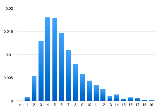
Fig. 3. $p_{0}^{2}(n)$, $\mu=1$, $\lambda=1,c=2,d=2$.

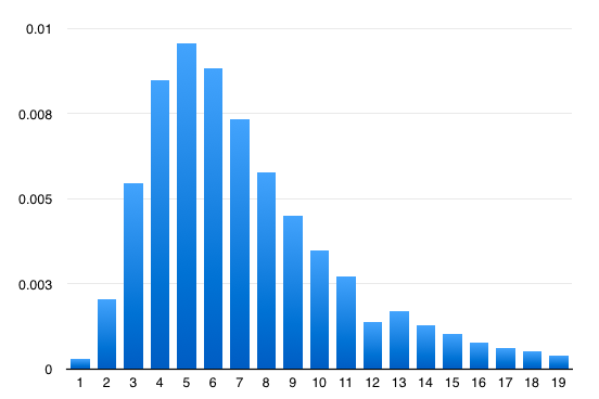
Fig. 4. $p_{1}^{2}(n)$, $\mu=1$, $\lambda=1,c=2,d=2$.

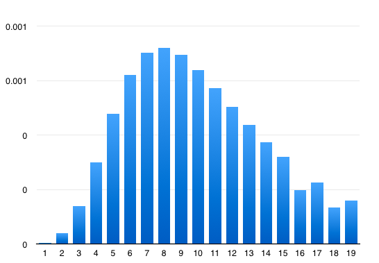
Fig. 5. $p_{5}^{2}(n)$, $\mu=1$, $\lambda=1,c=2,d=2$.

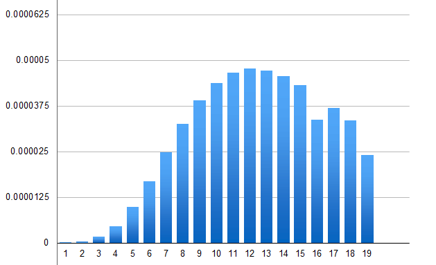
Fig. 6. $p_{10}^{2}(n)$, $\mu=1$, $\lambda=1,c=2,d=2$.

We noticed the following observations. The distributions are quite cumulated around the mode of $p_{u}^{d}(n)$ as a function $n$. Moreover, for fixed $u$, these probabilities first increase then decrease when the number of claims gets bigger. It seems the tails of this probability functions is surprisingly thick. In fact, it seems that larger $u$ produces thicker tail.

Now we will focus on more complex density $w_{u}^{d}(n,t)$. We will find it using Theorem 2.5.

From (20) it follows that:

$$w_{u}^{d}(1,t) = \lambda e^{-(\lambda+\mu c)t-\mu u}.$$ (33)

We will calculate now $w_{0}^{d}(n,t)$ for $n>1$ and $u=0$. Using 19 and (6) from we can derive the expression for $w_{0}^{d}(2,t)$:

$$w_{0}^{d}(2,t)=\left\{\begin{array}[]{lll}&\lambda^{2}e^{-(\lambda+\mu c)t}(\frac{1}{2}\mu ct^{2}+d-\frac{1}{2}\mu cd^{2}),&t>2d,\\ &\lambda^{2}e^{-(\lambda+\mu c)t}(\mu c(t-d)^{2}+d+\frac{1}{2}\mu cd^{2}),&d<t\leq 2d.\end{array}\right.$$ (36)

Similarly, using the expressions of $w_{0}^{d}(1,t)$ and $w_{0}^{d}(2,t)$ we can obtain the expression of $w_{0}^{d}(3,t)$:

$$w_{0}^{d}(3,t)=\left\{\begin{array}[]{lll}&\lambda^{3}e^{-(\lambda+\mu c)t}f_{31}(t),&t>3d,\\ &\lambda^{3}e^{-(\lambda+\mu c)t}f_{32}(t),&2d<t\leq 3d\\ &\lambda^{3}e^{-(\lambda+\mu c)t}f_{33}(t),&d<t\leq 2d,\end{array}\right.$$ (40)

where

$$f_{31}(t)=\frac{1}{24}[2c^{2}\mu^{2}t^{4}+(12cd\mu-6c^{2}d^{2}\mu^{2})t^{2}+4c^{2}d^{3}\mu^{2}t+12d^{2}-16cd^{3}\mu+5c^{2}d^{4}\mu^{2}],$$

$$f_{32}(t)=\frac{1}{24}[c^{2}\mu^{2}t^{4}+12c^{2}d\mu^{2}t^{3}+(12cd\mu-60c^{2}d^{2}\mu^{2})t^{2}+112c^{2}d^{3}\mu^{2}t+12d^{2}-16cd^{3}\mu-76c^{2}d^{4}\mu^{2}],$$

$$f_{33}(t)=\frac{1}{12}[3c^{2}\mu^{2}t^{4}-12c^{2}d\mu^{2}t^{3}+(12cd\mu+24c^{2}d^{2}\mu^{2})t^{2}-(24cd^{2}\mu+24c^{2}d^{3}\mu^{2})t+6d^{2}+16cd^{3}\mu$$

$$\ \ \ \ \ \ \ \ \ \ \ \ +10c^{2}d^{4}\mu^{2}].$$

This iterative algorithm can produce $w_{0}^{d}(n,t)$ for any $n>0$ and then by Theorem 2.5 we can identify all $w_{u}^{d}(n,t)$. Unfortunately, the computation process takes long time and the expression for $w_{u}^{d}(n,t)$ gets very complicated quite quickly. We suggest another numerical algorithm instead. We change the integration in the third increment of (24) and (22) into the summation using the rectangular method of approximating definite integrals. Of course taking the step of the summation tending to $0$ will give right expression.

Let $\lambda=1,\mu=1,c=1.2,d=2$. Here we divide up the interval $[0,10]$ into $100$ equal subintervals. Each has length $\Delta t=\dfrac{1}{10}$ . We will evaluate the function $w_{0}^{d}(n,t)$ at the right-hand endpoints of these subinterval. Figure 7 shows that the approximation is very good. We noticed that the time of calculating $w_{0}^{d}(n,t)$ is now much shorter. (Solid line denote the exactly values of the density function $w_{0}^{d}(n,t)$ and dotted line denote the approximate values.)

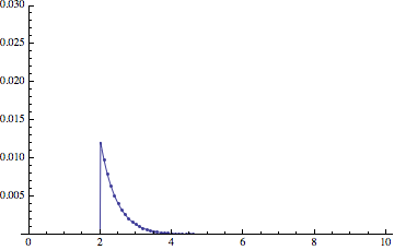
$w_{0}^{d}(1,t)$, $\mu=1$, $\lambda=1,c=1.2,d=2$.

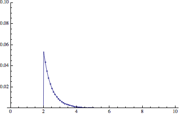
$w_{0}^{d}(2,t)$, $\mu=1$, $\lambda=1,c=1.2,d=2$.

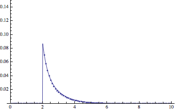
$w_{0}^{d}(3,t)$, $\mu=1$, $\lambda=1,c=1.2,d=2$.

Fig. 7. The exact and approximate values of $w_{0}^{d}(n,t)$.

Figure 8 shows the graphs for $w_{0}^{d}(n,t)$ for $n=1,2,3,4,5,6$ and Figure 9 shows the graphs for $w_{u}^{d}(n,t)$ when $d=2$, $u=2$. Tables $2-3$ give the values of $p_{0}^{d}(n,t)$ and $p_{u}^{d}(n,t)$ for $n=1,2,3,4,5,6$, $t=1,2,3,4,5,6,7$, respectively.

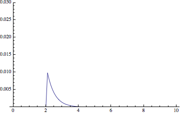
$w_{0}^{d}(1,t)$, $\mu=1$, $\lambda=1,c=1.2,d=2$.

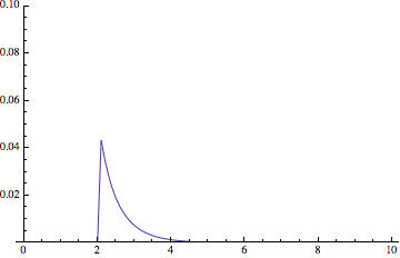
$w_{0}^{d}(2,t)$, $\mu=1$, $\lambda=1,c=1.2,d=2$.

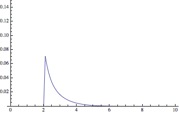
$w_{0}^{d}(3,t)$, $\mu=1$, $\lambda=1,c=1.2,d=2$.

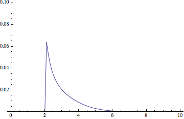
$w_{0}^{d}(4,t)$,$\mu=1$, $\lambda=1,c=1.2,d=2$.

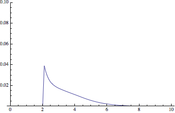
$w_{0}^{d}(5,t)$, $\mu=1$, $\lambda=1,c=1.2,d=2$.

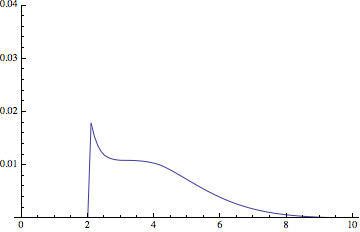
$w_{0}^{d}(6,t)$, $\mu=1$, $\lambda=1,c=1.2,d=2$.

Fig. 8. Graphs for $w_{0}^{d}(n,t)$, $\mu=1$, $\lambda=1,c=1.2,d=2$.

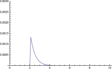
$w_{u}^{d}(1,t)$, $\mu=1$, $\lambda=1,c=1.2,d=2,u=2$.

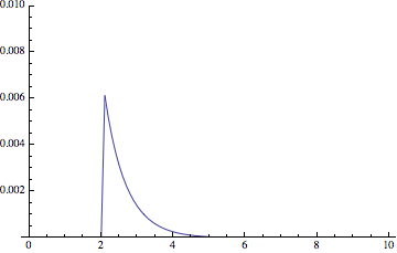
$w_{u}^{d}(2,t)$, $\mu=1$, $\lambda=1,c=1.2,d=2,u=2$.

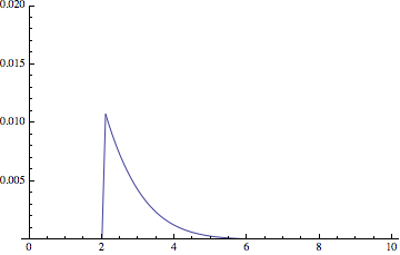
$w_{u}^{2}(3,t)$, $\mu=1$, $\lambda=1,c=1.2,d=2,u=2$.

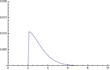
$w_{u}^{2}(4,t)$, $\mu=1$, $\lambda=1,c=1.2,d=2,u=2$.

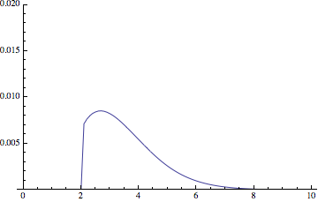
$w_{u}^{2}(5,t)$, $\mu=1$, $\lambda=1,c=1.2,d=2,u=2$.

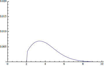
$w_{u}^{d}(6,t)$,$\mu=1$, $\lambda=1,c=1.2,d=2,u=2$.

Fig. 9. Graphs for $w_{u}^{d}(n,t)$, $\mu=1$, $\lambda=1,c=1.2,d=2,u=2$.

t	$t=1$	$t=2$	$t=3$	$t=4$	$t=5$	$t=6$	$t=7$
$n=1$	0	0	0.0044364	0.00492798	0.00498245	0.00498848	0.00498915
$n=2$	0	0	0.0204411	0.0236396	0.0242160	0.0243135	0.0243288
$n=3$	0	0	0.0360174	0.0445814	0.0469080	0.0474601	0.0475778
$n=4$	0	0	0.0360946	0.0494625	0.0548542	0.0566279	0.0571321
$n=5$	0	0	0.0246765	0.0386667	0.0468287	0.0505039	0.0518839
$n=6$	0	0	0.0127279	0.0234754	0.0323266	0.0377145	0.0403638
$n=7$	0	0	0.00527283	0.0117139	0.019034	0.0249818	0.0287784
$n=8$	0	0	0.00182873	0.00497309	0.00980279	0.0149746	0.0192228

Tab. 2. $p_{0}^{d}(n,t)$, $\mu=1$, $\lambda=1,c=1.2,d=2$.

t	$t=1$	$t=2$	$t=3$	$t=4$	$t=5$	$t=6$	$t=7$
$n=1$	0	0	0.000600403	0.000666929	0.000674301	0.000675117	0.000675208
$n=2$	0	0	0.00322483	0.00384155	0.00395467	0.00397339	0.00397626
$n=3$	0	0	0.00711875	0.00943587	0.0100615	0.0102047	0.0102339
$n=4$	0	0	0.00920644	0.0141209	0.0160422	0.0166421	0.016803
$n=5$	0	0	0.00816603	0.0149827	0.0187639	0.0203559	0.0209108
$n=6$	0	0	0.00542406	0.0122129	0.0174604	0.0204087	0.0217345

Tab. 3. $p_{u}^{d}(n,t)$, $\mu=1$, $\lambda=1,c=1.2,d=2,u=2$.

Acknowledgements
This research is support by the National Natural Science Foundation of China (Grant No. 11271164 and 11371020) and by the FP7 Grant PIRSES-GA-2012-318984. Zbigniew Palmowski is supported by the Ministry of Science and Higher Education of Poland under the grant 2013/09/B/HS4/01496.

References

- [1] R. E. Beard. On the calculation of the ruin probability for a finite time interval. ASTIN Bulletin, (6):129–133, 1971.
- [2] M. Chesney, M. Jeanblanc-Picqué, and M. Yor. Brownian excursions and Parisian barrier options. Advances in Applied Probability, pages 165–184, 1997.
- [3] I. Czarna and Z. Palmowski. Ruin probability with Parisian delay for a spectrally negative Lévy risk process. Journal of Applied Probability, 48(48):984, 2011.
- [4] A. Dassios and S. Wu. Parisian ruin with exponential claims. Manuscript, 2008.
- [5] D. C. M. Dickson. The joint distribution of the time to ruin and the number of claims until ruin in the classical risk model. Insurance: Mathematics and Economics, 50(3):334–337, 2012.
- [6] D. C. M. Dickson and G. E. Willmot. The density of the time to ruin in the classical Poisson risk model. Astin Bulletin, 35(1):45–60, 2005.
- [7] A. D. Egídio dos Reis. How many claims does it take to get ruined and recovered ? Insurance: Mathematics and Economics, 31:235–248, 2002.
- [8] E. Frostig, S. M. Pitts, and K. Politis. The time to ruin and the number of claims until ruin for phase-type claims. Insurance: Mathematics and Economics, 51(1):19–25, 2012.
- [9] H. U. Gerber and E. S. W. Shiu. The time value of ruin in a Sparre Andersen model. North American Actuarial Journal, 9(2):49–69, 2005.
- [10] J. L. Lagrange. Nouvelle méthode pour résoudre les équations littérales par le moyen des séries. Chez Haude et Spener, Libraires de la Cour & de l’Acad mie royale, 1770.
- [11] D. Landriault, J. F. Renaud, and X. Zhou. Occupation times of spectrally negative Lévy processes with applications. Stochastic Processes and Their Applications, 121(11):2629–2641, 2011.
- [12] D. Landriault, J. F. Renaud, and X. Zhou. An insurance risk model with Parisian implementation delays. Methodology and Computing in Applied Probability, 16(3):583–607, 2014.
- [13] D. Landriault, T. Shi, and G. E. Willmot. Joint densities involving the time to ruin in the Sparre Andersen risk model under exponential assumptions. Insurance: Mathematics and Economics, 49(3):371–379, 2011.
- [14] S. Li. The time of recovery and the maximum severity of ruin in a Sparre Andersen model. North American Actuarial Journal, 12(4):413–425, 2008.
- [15] R. Loeffen, I. Czarna, and Z. Palmowski. Parisian ruin probability for spectrally negative Lévy processes. Bernoulli, 19(2):599–609, 2013.
- [16] N. U. Prabhu. On the ruin problem of collective risk theory. Annals of Mathematical Statistics, 32(3):757–764, 1961.
- [17] D. A. Stanford and K. J. Stroiński. Recursive methods for computing finite-time ruin probabilities for phase-distributed claims. ASTIN Bulletin, 24:235–254, 1994.
- [18] C. Zhao and C. Zhang. Joint density of the number of claims until ruin and the time to ruin in the delayed renewal risk model with Erlang (n) claims. Journal of Computational and Applied Mathematics, 244:102–114, 2013.