Partial and Total Dielectronic Recombination rate coefficients for W⁷³⁺ to W⁵⁶⁺

Abstract

Dielectronic recombination (DR) is a key atomic process which affects the spectroscopic diagnostic modelling of tungsten, most of whose ionization stages will be found somewhere in the ITER fusion reactor: in the edge, divertor, or core plasma. Accurate DR data is sparse while complete DR coverage is unsophisticated (e.g. average-atom or Burgess General Formula) as illustrated by the large uncertainties which currently exist in the tungsten ionization balance. To this end, we present a series of partial final-state-resolved and total DR rate coefficients for W⁷³⁺ to W⁵⁶⁺ Tungsten ions. This is part of a wider effort within The Tungsten Project to calculate accurate dielectronic recombination rate coefficients for the tungsten isonuclear sequence for use in collisional-radiative modelling of finite-density tokamak plasmas. The recombination rate coefficients have been calculated with autostructure using kappa-averaged relativistic wavefunctions in level resolution (intermediate coupling) and configuration resolution (configuration average). The results are available from OPEN-ADAS according to the adf09 and adf48 standard formats. Comparison with previous calculations of total DR rate coefficients for W⁶³⁺ and W⁵⁶⁺ yield agreement to within 20% and 10%, respectively, at peak temperature. It is also seen that the Jüttner correction to the Maxwell distribution has a significant effect on the ionization balance of tungsten at the highest charge states, changing both the peak abundance temperatures and the ionization fractions of several ions.

I Introduction

ITER is posited to be the penultimate step in realizing a nuclear fusion power plant. It will be significantly larger than present machines, such as JET, in terms of plasma volume, core temperature, and physical size ITER Physics Basis Editors et al. (1999). Beryllium coated tiles will line the wall of the main reactor vessel due to their low erosion rate and the low tritium retention of Be. Tungsten ($Z=74$) will be used in regions of high power-loads, such as the divertor chamber at the base of the main vessel, and it is also resistant to tritiation El-Kharbachi et al. (2014). On the downside, such high-$Z$ elements are efficient radiators and must be kept to a minimum in the main plasma to avoid degrading its confinement. Because of this, JET has undergone a major upgrade to an ITER-like wall to act as a test-bed. Control of tungsten sources and its subsequent transport are under intensive study Fedorczak et al. (2015). Tungsten is the highest-$Z$ metal in widespread use in a tokamak. Prior to the installation of the ITER-like wall at JET, molybdenum ($Z=42$) was the highest-$Z$ metal in widespread use, at Alcator C-Mod. Like tungsten, molybdenum has a low tritium absorption rate Zakharov et al. (1975). However, molybdenum has a significantly lower melting point than tungsten, and also transmutes to technetium, complicating reactor decommissioning.

Most of the tungsten isonuclear sequence needs to be covered by non-LTE plasma modelling, from its initial sputtering from surfaces through the edge, divertor and core plasmas. One of the most basic quatities is the tungsten ionization balance: a measure of the dominant ionization stages as a function of temperature and density. While our understanding of the ionization rates required appears to be in reasonable order Loch et al. (2005), the same is not true for the competing dielectronic plus radiative recombination rates (DR+RR). In Figure 1 we compare the zero-density ionization balance for tungsten obtained using two different sets of recombination data Pütterich et al. (2008); Foster (2008) and the same ionization rate coefficients, of Loch et al. (2005). It can be seen that there are large discrepancies between the peak temperatures of individual ionization stages, as well as the fractional population of said ionization stage. The dielectronic recombination data of Pütterich et al Pütterich et al. (2008) was calculated with ADPAK Post et al. (1977, 1995) using an average-atom model and it was scaled by the authors in order to improve agreement between theory and experiment with regards to the shape of the fractional abundances of W²²⁺–W⁵⁵⁺. The DR data of Foster Foster (2008) used the Burgess General Formula Burgess (1965). Both used the same scaled hydrogenic radiative recombination data. Clearly, more reliable DR data is required.

Another issue is that the magnetic fusion plasmas cannot be taken to be a zero-density one. The true ionization balance is density dependent and the corresponding density dependent (effective) ionization and recombination rate coefficients are obtained from collisional-radiative modelling. The ionization rate coefficients are much less sensitive to density effects than the recombination ones because dielectronic recombination takes place through and to high-Rydberg states. Therefore, partial final-state-resolved rate coefficients are needed. Even where detailed calculations have been made, the data available is usually in the form of zero-density totals, i.e. summed-over all final states. As such, it is difficult to use such data for collisional-radiative modelling in reliable manner.

Detailed calculations have been performed for a select few ions of tungsten. However, these are very sparse, and tend to be for closed-shell ions which are important for plasma diagnostics. The most complicated exception to this to date is our work on the open f-shell: W^20+,18+ (4$d^{10}$ 4$f^{q},q=8,10$)Badnell et al. (2012); Spruck et al. (2014). Data for these ions were calculated using an upgraded version of autostructure designed to handle the increased complexity of the problem. The hullac Bar-Shalom et al. (2001) and the Cowan code Cowan (1981) have been used by Safronova et al Safronova et al. (2012, 2011); Safronova and Safronova (2012); Safronova et al. (2009a, b) to calculate DR rate coefficients for W⁵⁺, W²⁸⁺, W⁴⁶⁺, W⁶³⁺, and W⁶⁴⁺, respectively. Behar et al Behar et al. (1999) and Peleg et al Peleg et al. (1998) have also used these codes for W⁴⁶⁺,W⁶⁴⁺, and W⁵⁶⁺, respectively. In addition, the Flexible Atomic Code (fac, Gu (2003)) has been used by Meng et al Meng et al. (2009) and Li et al Li et al. (2012) to calculate DR rate coefficients for W⁴⁷⁺ and W²⁹⁺, respectively. Just recently, Wu et al Wu et al. (2015) have calculated zero-density total DR rate coefficients for W³⁷⁺ – W⁴⁶⁺ using fac.

In contrast, partial RR rate coefficients have been calculated for the entire isonuclear sequence of Tungsten, and the results presented in a series of papers, by Trzhaskovskaya et al Trzhaskovskaya et al. (2010); Trzhaskovskaya and Nikulin (2013, 2014a, 2014b). The authors used a Dirac-Fock method with fully relativistic wavefunctions, and included contributions from all significant radiation multipoles. The authors state that the majority of their RR rate coefficients were calculated to $<1$% numerical accuracy. However, for outer shell RR and high temperatures, their rate coefficients were calculated to $<5$% Trzhaskovskaya et al. (2010). The authors also present total RR rate coefficients summed up to $n=20$ and $\ell=19$.

In order to address this situation, we have embarked on a programme of work, as part of The Tungsten Project, which aims to calculate partial final-state resolved DR rate coefficients for use in collisional-radiative modelling with ADAS for the entire isonuclear sequence of tungsten. For completeness and ease of integration within ADAS, we compute the corresponding RR data at the same time. Zero-density totals are readily obtained from the archived data. The work presented here covers W⁷³⁺ to W⁵⁶⁺.

On a practical technical point, the names of various elements in the periodic table are not particularly helpful to label ionization stages of a large isonuclear sequence such as tungsten. Thus, we will not refer to such species by a name such as Pr-like. Instead, we adopt a notation based on the number of electrons possessed by a particular ion. For example, H-like (1 electron) W⁷³⁺ will be referred to as 01-like, Ne-like (10 electrons) W⁶⁴⁺ will be referred to as 10-like, and Pr-like (59 electrons) W¹⁵⁺ as 59-like. This mirrors our database archiving.

The outline of this paper is as follows: in Sec. II we outline the background theory for our description of DR and RR, as encapsulated in the autostructure code, and give consideration to the delivery of data in a manner appropriate for collisional-radiative modelling. In Sec. III, we describe our calculations for 00-like to 18-like ions. In Sec. IV, we present our results for DR/RR rate coefficients and compare them with those published previously, where available; then we look at how the zero-density ionization balance of tungsten changes on using our new recombination data. We conclude with some final remarks, and outline future calculations.

II Theory

We use the distorted-wave atomic package autostructure Badnell (1986, 1997, 2011). For recombination, autostructure makes use of the independent processes and isolated resonance approximations Pindzola et al. (1992). Then, the partial DR rate coefficient ${}^{DR}\alpha_{f\nu}^{z+1}$, from some initial state $\nu$ of ion $X^{+z+1}$ to a final state $f$ of ion $X^{+z}$, can be written as

$${}^{DR}\alpha_{f\nu}^{z+1}(T_{e})=\left(\frac{4{\pi}a_{0}^{2}I_{H}}{k_{B}T_{e}}\right)^{\frac{3}{2}}\sum_{j}\frac{\omega_{j}}{2\omega_{\nu}}\exp{\left[-\frac{E}{k_{B}T_{e}}\right]}\frac{\sum_{l}{A_{j\rightarrow{\nu},E\,l}^{a}}{A_{j\rightarrow{f}}^{r}}}{\sum_{h}{A_{j\rightarrow{h}}^{r}}+\sum_{m,l}{A_{j\rightarrow{m},E\,l}^{a}}},$$ (1)

where the $A^{a}$ are the autoionization rates, $A^{r}$ are the radiative rates, $\omega_{j}$ is the statistical weight of the $N$-electron target ion, $E$ is the total energy of the continuum electron, minus its rest energy, and with corresponding orbital angular momentum quantum number $l$ labelling said channels. $I_{H}$ is the ionization energy of the hydrogen atom, $k_{B}$ is the Boltzmann constant, $T_{e}$ is the electron temperature, and $(4{\pi}a_{0}^{2})^{3/2}=6.6011\times{10}^{-24}$cm³. The sum over the autoionizing states $j$ recognizes the fact that, in general, these states have sufficiently short lifetimes in a magnetic fusion plasma for them not be collisionally redistributed before breaking-up, although statistical redistribution is assumed in some cases Badnell (2006).

The partial RR rate coefficient ${}^{RR}\alpha_{f\nu}^{z+1}$ can be written, in terms of the photoionization cross section ${}^{PI}\sigma_{\nu f}^{z}$ for the inverse process using detailed balance, as

$${}^{RR}\alpha_{f\nu}^{z+1}(T_{e})=\frac{c\,\alpha^{3}}{\sqrt{\pi}}\frac{\omega_{f}}{2\omega_{\nu}}\left(I_{H}k_{B}T_{e}\right)^{-3/2}\int^{\infty}_{0}E^{2}_{\nu f}\,{{}^{PI}\sigma_{\nu f}^{z}(E)}\exp{\left[-\frac{E}{k_{B}T_{e}}\right]}dE\,,$$ (2)

where $E_{\nu f}$ is the corresponding photon energy and $c\,\alpha^{3}/\sqrt{\pi}=6572.67$cm s^-1 for ${}^{PI}\sigma_{\nu f}^{z}$ given in cm². The photoionization cross sections for arbitrary electric and magnetic multipoles are given by Grant (1974). The numerical approaches to converging the quadrature accurately and efficiently have been given previously Badnell (2006).

At high temperatures ($\gtrsim 10^{9}$ K) relativistic corrections to the usual Maxwell-Boltzmann distribution become important. The resultant Maxwell-Jüttner distribution Synge (1957) reduces simply to an extra multiplicative factor, $F_{\mathrm{r}}(\theta)$, to be applied to the Maxwell-Boltzmann partial rate coefficients:

$$F_{\mathrm{r}}(\theta)=\sqrt{\frac{\pi\theta}{2}}\frac{1}{K_{2}(1/\theta){\rm e}^{1/\theta}},$$ (3)

where $\theta=\alpha^{2}k_{B}T/2I_{H}$, $\alpha$ is the fine-structure constant and $K_{2}$ is the modified Bessel function of the second kind. This factor is normally consistently omitted from data archived in ADAS, being subsequently applied if required in extreme cases. However, since it has a non-negligible affect at the temperature of peak abundance for the highest charge states we consistently include it for all tungsten DR and RR data and flag this in the archived files.

Plasma densities in magnetic fusion reactors vary greatly. For ITER, the plasma densities are thought to vary from $10^{10}$–$10^{13}$ cm^-3 for the edge plasma, to $\sim{10}^{14}$ cm^-3 for the core plasma, reaching $\sim{10}^{15}$ cm^-3 for the divertor plasma. Because of these densities, the coronal picture breaks down: capture into an excited state does not cascade down to the ground uninterrupted. Instead, further collisions take place, leading in particular to stepwise ionization, for example. This strongly suppresses coronal total recombination rate coefficients. Collisional-radiative (CR) modelling of the excited-state population distribution is necessary. This leads to density-dependent effective ionization and recombination rate coefficients. A key ingredient for CR modelling is partial final-state-resolved recombination data. Our approach for light systems is detailed in Badnell et al. (2003) and Badnell (2006) for DR and RR, respectively. Low-lying final-states are fully level-resolved while higher-lying states are progressively ($n\ell$- and $n$-) bundled over their total quantum numbers, whilst retaining their level parentage. Initial ground and metastable levels are also fully-resolved. The data are archived in ADAS standard formats, viz. adf09 (DR) and adf48 (RR). One does not need to progress far into the M-shell for the number of such final states to become unmanageable by CR modelling and further bundling is required. This is carried-out most efficiently as the partial recombination rate coefficients are calculated and leads to much more compact adf09 and adf48 files. We find it necessary to bundle over all final recombined levels within a configuration. For such configurations which straddle the ionization limit we include the statistical fractions within the adf files. The initial ground and metastable levels remain level-resolved, as does the calculation of autoionizing branching ratios (fluorescence yields). We describe such a mixed resolution scheme as a ‘hybrid’ approach and the adf files are labelled accordingly. All resultant adf09 and adf48 files are made available via OPEN-ADAS .

III Calculations

All rates and cross sections were determined on solving the kappa-averaged quasi-one-electron Dirac equation for the large and small components utilizing the Thomas-Fermi-Dirac-Amaldi model potential Eissner and Nussbaumer (1969) with unit scaling parameters to represent the $N$- and $(N+1)$-electron ions. We utilized several coupling schemes. Configuration average (CA) was used to give a quick overview of the problem. This neglects configuration mixing and relativistic interactions in the Hamiltonian. $LS$-coupling (LS) allows for configuration mixing but tends to overestimate it in such highly-charged ions because relativistic interactions push interacting terms further apart. Thus, our main body of data is calculated in intermediate coupling (IC). For the K-shell ions, we included valence-valence two-body fine structure interactions. These gave rise to a $\sim$7% increase in the total DR rate coefficients for 01-like and 02-like ions at high temperatures. We neglect these interactions for the L- and M-shell ions since the increase in the total DR rate coefficient is $<1$%.

III.1 DR

It is necessary to include all dominant DR reactions illustrated by Eq.(1). The initial state $\nu$ is taken to be the ground state. Metastables are unlikely to be important at such high charge states. The driving reactions are the autoionizing states produced by one-electron promotions from the ground configuration, with a corresponding capture of the continuum electron. We label these core-excitations by the initial ($n$) and final ($n^{\prime}$) principal quantum numbers of the promoted electron, and include all corresponding sub-shells ($\ell$-values). The dominant contributions come from $\Delta n=0$ ($n=n^{\prime}$) and $\Delta n=1$ ($n^{\prime}=n+1$), being well separated in energy/temperature. Contributions from $\Delta n>1$ tend to be suppressed by autoionization into excited states, as represented by the sum over $A^{a}$ in the denominator of (1). The outermost shell dominates but the $\Delta n=1$ inner-shell promotion ($n=n^{\prime}-1$) can be significant when there are few outer $n$-shell electrons. As their number increases, core re-arranging autoionizing transitions suppress this inner-shell contribution. These core-excitations define a set of $N$-electron configurations to which continuum and Rydberg electrons are coupled.

Based-on these promotion rules, the core-excitations considered for each ion (W⁷³⁺ to W⁵⁶⁺) are listed in Table LABEL:table:drcorex. The calculations were carried-out first in CA to determine which excitations are dominant. We omitted core-excitations that contribute $<1$% to the sum total of all DR core-excitation rate coefficients spanning the ADAS temperature grid. This grid covers $10z^{2}$–$2\times{10}^{6}z^{2}$ K, where $z$ is the residual charge of the initial target ion. DR for the dominant core-excitations is then calculated in IC. The $n\ell$ Rydberg electron, in the sum over autoionizing states $j$, is calculated explicitly for each principal quantum number up to $n=25$ and then on a quasi-logarithmic $n$-mesh up to $n=999$. The partial DR rate coefficient tabulation is based on this mesh of $n$-values. Total (zero-density) DR rate coefficients are obtained by interpolation and quadrature of these partials. The maximum Rydberg orbital angular momentum ($\ell$) is taken to be such that the total rate coefficients are converged to better than 1% over the ADAS temperature range. Radiative transitions of the Rydberg electron to final states with principal quantum number greater than the core-excitations’ are described hydrogenically. Those into the core are described by a set of $(N+1)$-electron configurations which are generated by adding another core electron orbital to all $N$-electron configurations describing the core-excitations. In the case of $\Delta n>1$ core-excitations this also allows for dielectronic capture into the core.

To make clear to the complete set of configurations included for a typical calculation, we give a list of configurations used to calculate DR rate coefficients for 14-like $3-3$ and $3-4$ core-excitations in Table LABEL:table:14likeconf. We have marked also, with an *, configurations which were added to allow for the dominant configuration mixing within a complex by way of the ‘one up, one down rule’. For example, the configuration $3s3p^{2}3d$ strongly mixes with $3p^{4}$ and $3s^{2}3d^{2}$.

III.2 RR

The partial RR rate coefficients were calculated in a similar, but simplified fashion, to $\Delta{n}=0$ DR, viz., the $N$-electron target configurations were restricted to those which mixed with the ground and the $(N+1)$-electron configurations were these $N$-electron configurations with an additional core electron. The Rydberg $n\ell$-values were again calculated for each $n$ up to $n=25$ and then on the same $n$-mesh as used for DR, up to $n=999$, with $\ell=0-10$, relativistically. At high-$T$ ($>10^{9}$) K, many multipoles contribute to the photoionization/recombination at correspondingly high energies Pratt et al. (1973). We included up to E40 in CA and E40/M39 in the IC calculations, which is sufficient to converge the total RR rate coefficients to $<1$% over the ADAS temperature range. A non-relativistic (dipole) top-up was then used to include up to $\ell=150$ to converge the low-temperature RR rate coefficients — relativistic effects being negligible there. This approach is sufficient to calculate the total RR rate coefficients to better than 1%, numerically.

IV Results and Discussion

In this section we present the results of our DR and RR rate coefficient calculations for 00-like to 18-like. In our plots we show the tungsten fractional peak abundance curves from Pütterich et al Pütterich et al. (2008) to give an indication of the relevant temperatures for application purposes. At these temperatures, RR is dominated by capture into the lowest available $nl$-subshell. We consider the DR rate coefficients first, and look at the K, L, and M shells in turn. Next, we consider the RR rate coefficients, and assess their importance relative to DR. We compare our results with others, where possible. Finally, we look at the effect on the zero-density ionization balance of tungsten when using our new data.

IV.1 K-shell DR

The DR rate coefficients for 01 and 02-like are very small compared to RR. The reason for this is that the RR rate coefficient scales as $z$ (residual charge) while the DR rate coefficient here scales as $z^{-3}$, being proportional to the dielectronic capture rate (the fluorescence yields are close to unity due to the $z^{4}$ scaling of the radiative rates and the $z^{0}$ ($=1$) of the autoionization.) In Figure  2 we have plotted the DR and RR rate coefficients for 01-like. In the top subplot, we show the individual contributions from each DR core-excitation, and RR. The ionization balance for 01-like, calculated using the scaled recombination data of Pütterich et al Pütterich et al. (2008) and the ionization data of Loch et al Loch et al. (2005), is plotted also for reference. In the bottom subplot, we have plotted the cumulative sum of each contribution to the total recombination rate coefficient. This was calculated by taking the fraction of the largest contribution to the total recombination rate coefficient. The next curve is calculated by adding the first and second largest contributions together, and taking the fraction of this to the total recombination rate coefficient, and so on. It can be seen that the total recombination rate coefficient is dominated by RR, it being at least two orders of magnitude larger than DR at any temperature of interest. Comparatively, the DR $\Delta{n}=1$ core-excitations for 01- and 02-like are a factor 10 larger than their corresponding $\Delta{n}=2$ core-excitations. This is due to the (core) $n^{-3}$ scaling of the autoionization rate, rather than $\Delta{n}=1$ autoionization into excited states for the $\Delta{n}=2$. Finally, in Figure 3 we compare the total 01- and 02-like DR rate coefficients. The 02-like is roughly a factor of two larger because there are two K-shell electrons available to promote.

IV.2 L-shell DR

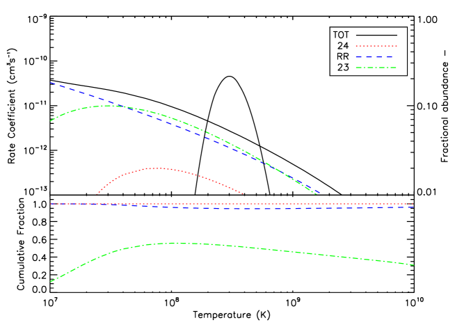
Figure 5: As Figure 2, but for 10-like with core-excitations 2-3 and 2-4.

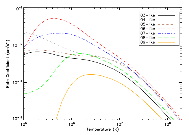
Figure 6: DR rate coefficients for 2-2, $\Delta{n}=0$ core-excitation for 03- to 09-like.

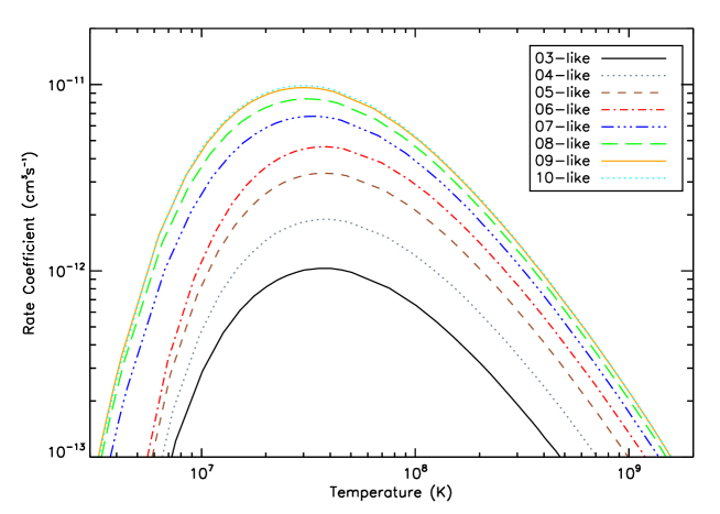
Figure 7: DR rate coefficients for 2-3, $\Delta{n}=1$ core-excitation for 03- to 10-like.

In Figure 4 we have plotted the DR and RR rate coefficients for 03-like in a similar manner to Figure 2. The RR rate coefficient drops by a factor of two due to the K-shell being closed while dominant (for DR) contributions arise from the 2-2 and 2-3 core-excitations. Nevertheless, RR still contributes $\sim 60-90$% of the total recombination rate coefficient around the temperature of peak abundance. As the L-shell fills, the total RR rate coefficient decreases due to decreasing L-shell vacancy (and charge somewhat) while the DR increases correspondingly due to the increasing number of electrons available to be promoted. The two become comparable at 10-like (see Figure 5) when the RR can only start to fill the M-shell. In Figures 6 and 7 we have plotted the DR rate coefficients for the 2-2 and 2-3 core excitations respectively, with the former covering 03- to 09-like and the latter covering 03- to 10-like. The 2-2 core-excitation provides the largest contribution to the total DR rate coefficients when filling the $2s$ shell. After the $2p$ subshell is half filled (06-like), the 2-2 DR rate coefficient decreases gradually, being overtaken by the 2-3 core-excitation. The 2-4 core-excitation provides only a small contribution in 03- and 04-like ($<1$% at peak abundance), and was hence neglected from 05-like onwards. In 10-like, the 2-4 core excitation was re-introduced as a consistency check now that the 2-2 is closed, however, it still provides a minimal contribution of $\sim$5% around peak abundance.

IV.3 M-shell DR

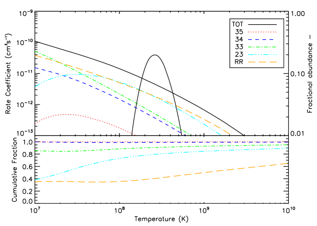
Figure 8: As Figure 2, but for 11-like with core-excitations 2-3, 3-3, 3-4, and 3-5.

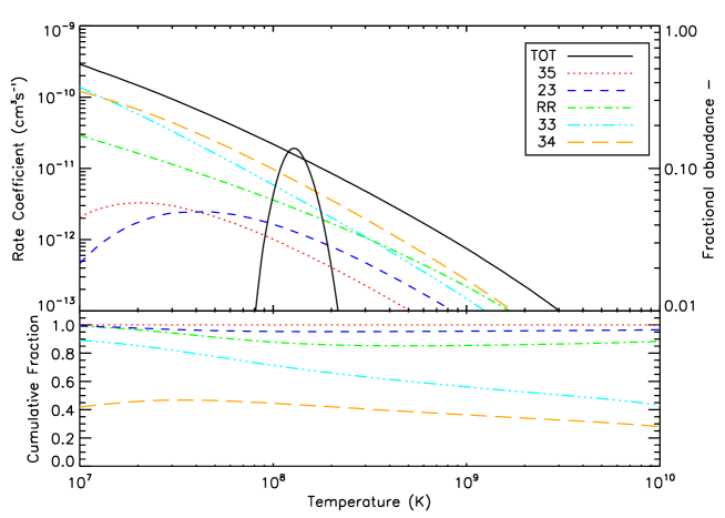
Figure 9: As Figure 2, but for 18-like with core-excitations 2-3, 3-3, 3-4, and 3-5.

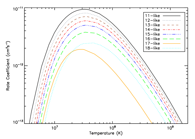
Figure 10: DR rate coefficients for 2-3, $\Delta{n}=1$ core-excitation for 11- to 18-like.

A temperature of 26keV ($3\times{10}^{8}$K) corresponds to the peak abundance of 10-like W. Higher charge states will exist, with increasingly small fractional abundance, but may be seen spectroscopically. The M-shell is perhaps the deepest shell in tungsten that ITER will be able to access routinely. The M-shell is also the regime in which RR increasingly gives way to DR, contributing $\sim$40% of the total recombination rate coefficient in 11-like, and decreasing to $\sim$15% in 18-like, around the temperature of peak abundance (see Figures 8 and 9, respectively). The inner-shell 2-3 core-excitation provides the largest contribution to the total DR rate coefficient in 11-like ($\sim{40}$%), however, this is quickly overtaken by the $\Delta{n}$=0 and outer shell $\Delta{n}$=1 core-excitations of 3-3 and 3-4, respectively. Again, this can be understood in terms of a simple occupancy/vacancy argument. In addition, the 2-3 is increasingly suppressed by core re-arrangement autoionizing transitions, viz. an M-shell electron drops down into the L-shell and ejects another M-shell electron. This process is independent of the Rydberg-$n$, unlike the initial dielectronic capture. The reduction of the 2-3 core-excitation DR with increasing M-shell occupation is shown in Figure 10, where we have plotted the 2-3 DR rate coefficients for 11-like to 18-like.

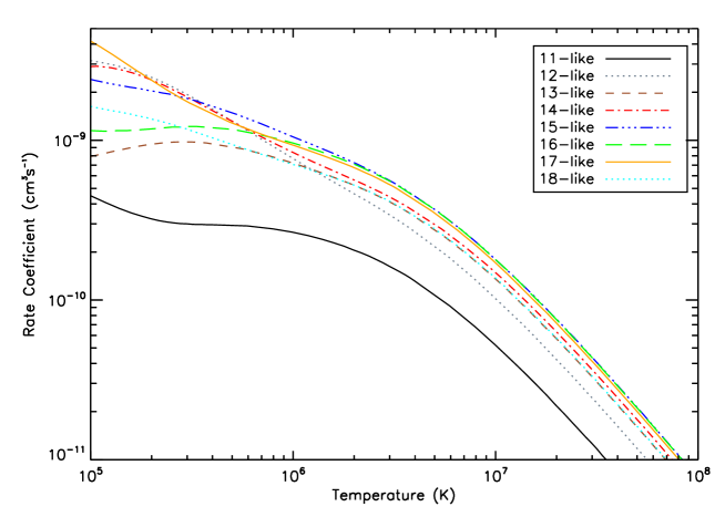
Figure 11: DR rate coefficients for 3-3, $\Delta{n}=0$ core-excitation for 11- to 18-like.

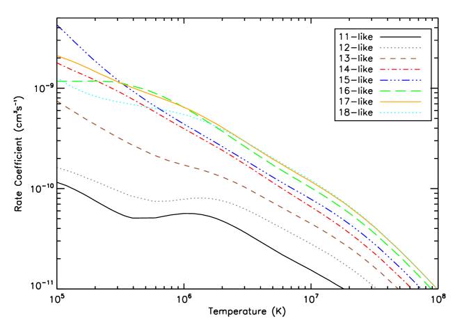
Figure 12: DR rate coefficients for 3-4, $\Delta{n}=1$ 3-4 core-excitation for 11- to 18-like.

The outer-shell $\Delta{n}$=0 (3-3) and $\Delta{n}$=1 (3-4) core-excitations provide the largest contributions to the total recombination rate coefficients from 12-like onwards. In Figure 11, we have plotted the ($3p^{q}$) 3-3 core-excitations for 11-like to 18-like, where there is competition between $3p$ occupancy and $3p$ vacancy. It can be seen that the 3-3 contribution grows steadily up to 15 and 16-like reaching a maximum value there. The rate coefficient then begins to decrease for 17- and 18-like as the $3p$ shell closes, leaving only $3d$ vacancies. In Figure 12 we have plotted the 3-4 DR rate coefficients for 11-like to 18-like. The 3-4 rate coefficients increase simply with increasing $3p$ occupancy.

The $\Delta{n}$=2 (3-5) core-excitation again provides only a small contribution throughout 11- to 18-like. This contribution is at its smallest for 11-like (Figure  8), contributing $\sim{1}$% to the total recombination rate coefficient. As with 3-4, the 3-5 DR rate coefficient increases up to 17- and 18-like, but still only contributes $\sim{5}$% for the final ion. Despite the small contribution, we opted to keep the 3-5 core-excitation as the 2-3 one decreases rapidly with the filling of the $3p$ shell.

IV.4 Relativistic Configuration Mixing in DR

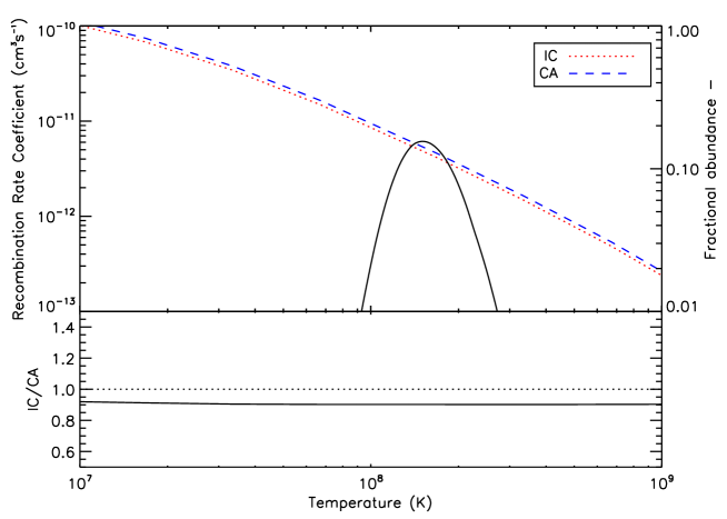
Figure 13: Total DR rate coefficients for 16-like 3-4. The bottom plot shows the ratio of the IC coefficients to CA. The dotted line indicates a ratio of unity.

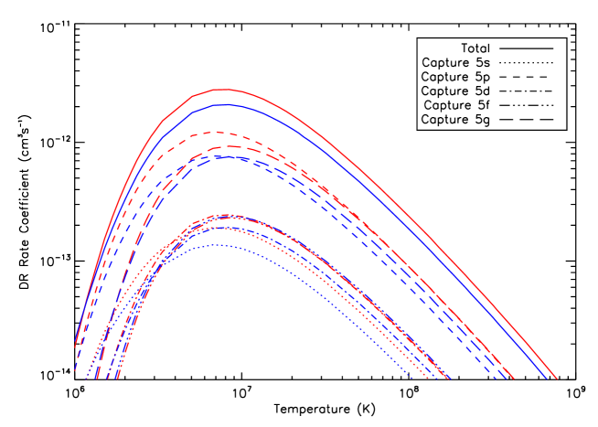
Figure 14: Partial DR rate coefficients for 16-like 3-4 capture to $n=5$ for subshells $5s-5g$. The red curves correspond to the CA calculation, while the blue correspond to IC.

Comparing total DR rate coefficients, although convenient, can be somewhat misleading since non-relativistic configuration mixing and relativistic (e.g. spin-orbit) mixing are described by unitary transformations of the initial basis wavefunctions. For example, in Figure 13 we show the total DR rate coefficients for the 16-like 3-4 core-excitation calculated in IC and CA. It can be seen the agreement between IC and CA is very good, being $\sim{10}$% around the temperature of peak abundance. Now, if we consider a set of partial DR rate coefficients for 16-like 3-4, we can see the agreement between IC and CA is much worse. In Figure 14 we have plotted the partial DR rate coefficients for 16-like 3-4, capture to $n=5$. The best agreement is for recombination into the $5f$, with IC and CA differing by $\sim{5}$%. The worst agreement is seen for recombination into $5p$, where the IC and CA rate coefficients differ by $\sim{33}$% at peak abundance. Agreement is no better for $5s$, $5d$, and $5g$, where the IC and CA rate coefficients differ by $\sim{28}$%, $\sim{19}$%, and $\sim{18}$% respectively.

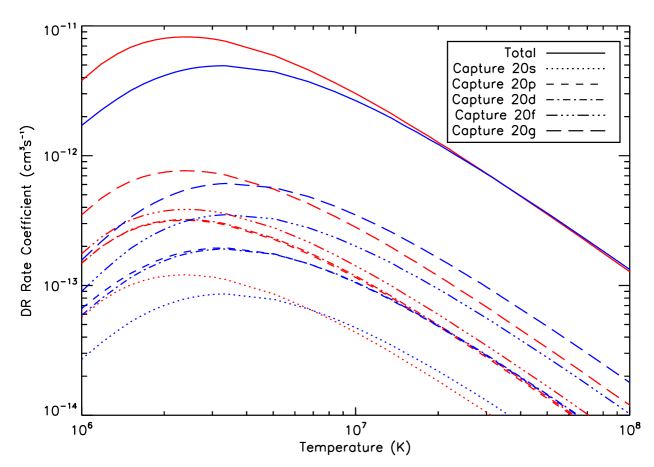
Figure 15: Partial DR rate coefficients for 16-like 3-3 capture to $n=20$ for subshells $20s-20g$. The red curves correspond to the CA calculation, while the blue correspond to IC.

The disagreement between partial DR rate coefficients calculated in IC and CA is even more apparent when considering the 3-3 core-excitation. In Figure 15 we have plotted the partial DR rate coefficients for 16-like 3-3, capture to $n=20$. The best agreement occurs for $20p$ and $20d$, where the partials differ by $<10$% at peak abundance. The same cannot be said for $20s$, $20f$, and $20g$, where the IC and CA results differ by $\sim{30}$%, $\sim{72}$%, and $\sim{51}$% respectively. These differences highlight the importance of relativistic mixing for a heavy atom such as tungsten. This effect is not confined to 16-like, and occurs for all ions considered in this work. Its subsequent propagation through collisional-radiative modelling is a topic for future study.

IV.5 Comparison with other DR work

With the exception of closed-shell ions, not much DR rate coefficient data has been calculated for the ions W⁷³⁺ to W⁵⁶⁺. As ITER will have an operating temperature of up to $\sim{26}$keV ($\sim{3}\times{10}^{8}$K), the reactor will be able to access to about 10-like W⁶⁴⁺. In Tables LABEL:table:beharcomp and LABEL:table:safronovacomp we compare our total DR rate coefficients for 10-like with those of Behar et al Behar et al. (1999) and Safronova et al Safronova et al. (2009b) respectively, both of whom used the hullac Bar-Shalom et al. (2001) code. Agreement with the results of Behar et al is generally good, being $\sim{10}$% near peak abundance, while low temperatures illustrate the characteristic sensitivity of DR rate coefficients to near-threshold resonances. However, a significant difference is noted between these two sets of results and those of Safronova et al , where our DR rate coefficients are larger by $\sim$50% for temperatures $>2\times{10}^{8}$K. The origin of this difference is currently unknown. In Table LABEL:table:pelegcomp we compare our 18-like total DR rate coefficients with the hullac ones of Peleg et al Peleg et al. (1998). Agreement is better in this case over a wider range of temperatures, being $\lesssim$10% at peak abundance.

IV.6 RR

In Figure 16 we show our total RR rate coefficients from 00-like to 18-like calculated in IC. These include all multipoles up to E40/M39 and the Jüttner relativistic correction. The pattern of curves seen corresponds to the filling of the K-shell and then the L-/M-shell boundary, as noted above. As mentioned previously, Trzhaskovskaya et al Trzhaskovskaya et al. (2010); Trzhaskovskaya and Nikulin (2013, 2014a, 2014b) have calculated an extensive set of partial and ‘total’ (summed to $n=20$, $\ell=19$) RR rate coefficients for the whole tungsten isonuclear sequence. Their calculations were fully relativistic, extending to $n=20$, $\ell=19$. Comparatively, our autostructure calculations extend to $n=999$ and $\ell=150$, where values up to $\ell=10$ were treated relativistically in the kappa-averaged approximation. A non-relativistic dipole top-up was then used to cover the remaining $\ell$ values which become important at low (non-relativistic) temperatures. In Table LABEL:table:trzcomp we compare the RR rate coefficients of Trzhaskovskaya et al Trzhaskovskaya et al. (2010) for 00-like (fully stripped) to ours over log $T\mathrm{(K)}$ of 3.0 to 10.0. In this table, we have given our rate coefficients when summed up to $n=999$ and $\ell=150$, as well as the rate coefficients when summed up to $n=20$ and $\ell=19$. In the case where we do not truncate $n$ and $\ell$ we see very large differences at low temperatures ($>100$% for log $T\mathrm{(K)}\leq{3.5}$.) This difference decreases steadily until $\sim{10^{9}}$K, where it then begins to increase again. When we truncate our $n$ and $\ell$ values to match Trzhaskovskaya et al , we find excellent agreement between the two data sets for log $T\mathrm{(K)}<9.5$ ($<1$%). Above log $T\mathrm{(K)}=9.5$ we note a slight drift away from the results of Trzhaskovskaya et al , reaching $\sim{10}$% at the highest temperature log $T\mathrm{(K)}$=10.0. This is likely due to the use of kappa-average wavefunctions by autostructure, assuming $<1\%$ accuracy in the results of Trzhaskovskaya et al still. The kappa-average approximation begins to break down at high temperatures, or rather at the corresponding high electron energies which contribute at such $T$. The underlying photoionization cross sections are falling-off rapidly in magnitude and such small quatities become increasingly sensitive to the kappa-average approximation. Such a difference at these temperatures should be of no importance to modelling. But, it is useful to have a complete set of consistent partial RR data to complement the DR data for collisional-radiative modelling with ADAS. As already noted, RR is most important for the highest few ionization stages. By 10-like, the total DR rate coefficient is comparable to RR at the temperature of peak abundance. By 18-like, the RR rate coefficient contributes only $\approx 10$% to the total rate coefficient at peak abundance.

IV.7 Comparison with Pütterich et al & Foster DR+RR

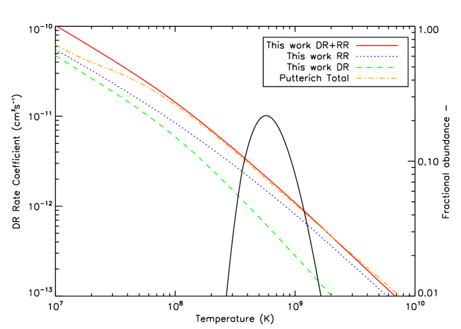
Figure 19: Comparison of the present separate DR and RR rate coefficients, together with their sum total, with the total rate coefficients of Pütterich et al Pütterich et al. (2008) for 06-like.

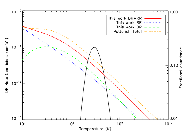
Figure 20: As Figure 19, but for 10-like.

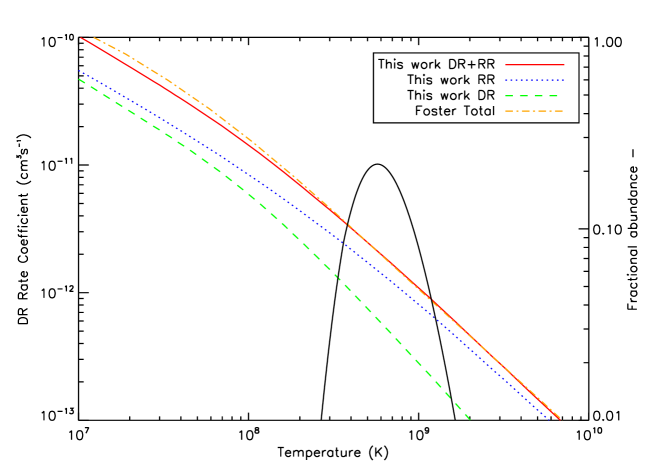
Figure 21: Comparison of the present separate DR and RR rate coefficients, together with their sum total, with the total rate coefficients of Foster Foster (2008) for 06-like.

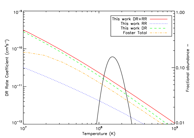
Figure 22: Same as Figure 21, but for 16-like.

The Pütterich et al Pütterich et al. (2008) DR data is ADPAK Post et al. (1977, 1995), which uses an average-atom method, and was further scaled for W²²⁺–W⁵⁵⁺. The Foster Foster (2008) DR data was calculated using the Burgess General Formula Burgess (1965). Both use the same ADAS RR data, which is scaled hydrogenic. We now compare our DR+RR results with those Pütterich et al and Foster. In order to do this, we omit the Jüttner relativistic correction from our recombination rate coefficients, as they did. On comparing our recombination rate coefficients with Pütterich et al , we find that there are multiple ions where there is good agreement. For example, in Figure 19 we have plotted the 06-like recombination rate coefficients for Pütterich et al , and our DR and RR rate coefficients and their sum. We find our rate coefficients are in agreement with those of Pütterich et al to $<$10% at peak abundance. Some ions are in poor agreement. In Figure 20 we compare our recombination rate coefficients with those of Pütterich et al for 10-like. The agreement is very poor at peak abundance with a difference of $>$40%. For the Foster data, good agreement is again seen in multiple ions. In Figure 21 we plot our DR, RR, and total recombination rate coefficients along with Foster’s total (DR+RR) rate coefficients for 06-like. The difference between ours and Foster’s rate coefficient is even smaller than found with Pütterich et al , being $<$1% at peak abundance. The largest disagreement between ours and Foster’s data occurs for 16-like. We have plotted ours and Foster’s recombination rate coefficients for 16-like in Figure 22. Poor agreement can be seen across a wide temperature range. At peak abundance, ours and Foster’s recombination rate coefficients differ by $>$40%.

The agreement between our present total DR plus RR rate coefficients and those of Foster Foster (2008) is similar to the agreement between ours and those of Pütterich et al Pütterich et al. (2008) for 01-like to 11-like, with the differences being $<$30% near peak abundance. For 12-like and beyond, the Pütterich et al recombination data is in better agreement with ours, while Foster’s data is consistently smaller than ours. As previously noted, DR becomes increasingly important as we move from the L-shell to the M-shell. Thus, crude/simple methods such as average-atom and the Burgess General Formula can give good descriptions of DR, but also very poor ones. Also, they are not readily adaptable to delivering the partial final-state-resolved data required for collisional-radiative modelling, although the Burgess General Program underlying his General Formula can do so.

IV.8 Ionization balance

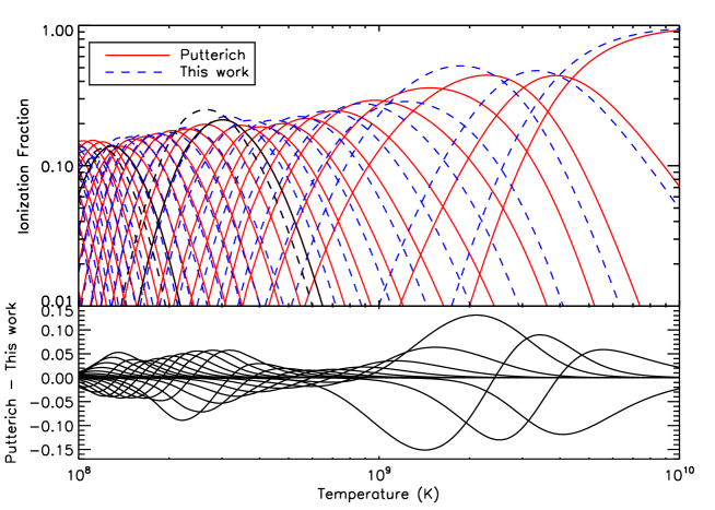
Figure 17: Zero-density fractional abundances of tungsten ionization stages, calculated using Pütterich et al Pütterich et al. (2008) recombination data (red, solid curves) and the present recombination data (blue, dashed curves). The black curves, from right to left, indicate 10-like and 18-like. Both use the ionization rate coefficients from Loch et al Loch et al. (2005).

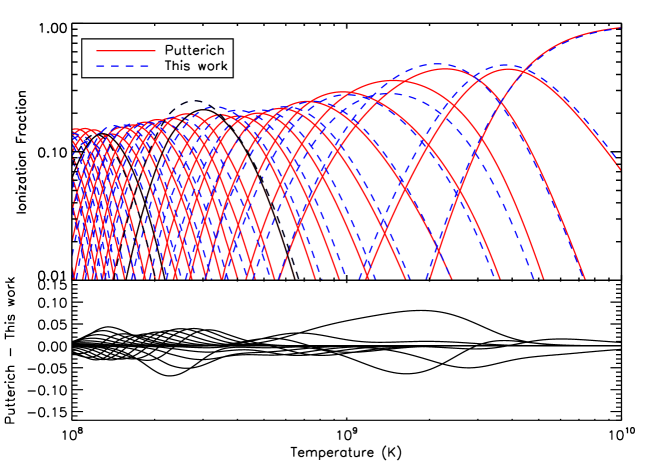
Figure 18: As Figure 17, but with the Jüttner correction removed from our data.

In order to compare the effect of our new recombination data, on the zero-density ionization balance, with that of Pütterich et al Pütterich et al. (2008), we replaced their recombination data with our new DR+RR data for 00-like to 18-like tungsten. In Figure 17, we compare the ionization balance obtained with this new data set with the original one of Pütterich et al . A large discrepancy is immediately apparent, namely that our peak abundance fractions have shifted relative to those of Pütterich et al . This has a simple explanation, in that our data has the Jüttner relativistic correction applied. By excluding this correction, our ionization fraction moves into better agreement with the Pütterich et al fraction, as seen in Figure 18.

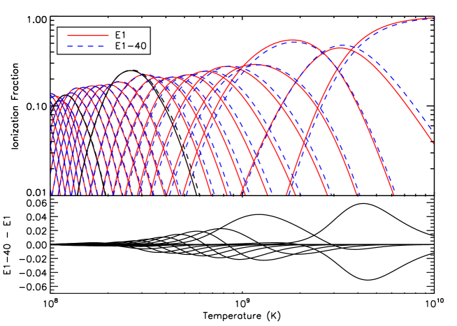
Figure 23: Zero-density fractional abundances of tungsten ionization stages, calculated using RR rate coefficients with dipole only (red, solid curves) and E1-40/M39 multipoles included (blue, dashed curves). All this work.

Electric and magnetic multipole radiation contributions to the RR rate coefficients become important at high temperatures Pratt et al. (1973). In Figure 23 we have plotted the ionization balance using RR rate coefficients where only electric dipole radiation is included, and using RR rate coefficients where electric and magnetic multipoles up to E40 and M39 have been included. The inclusion of higher multipoles increases the peak abundance temperature of the highest-charge ions as expected, however, the peak abundance temperature only changes by $\sim{4}$% for 01- and 02-like. This shift decreases rapidly to zero towards 18-like as DR becomes dominant over RR.

V Conclusion

Large uncertainties exist in the tungsten ionization balance over a wide range of temperatures (charge-states) found in magnetic fusion plasmas. This ranges from the cool edge plasma right through to the hot core plasma. The cause is the simplified treatment of DR, using either the average-atom or Burgess General Formula approaches. We have embarked on a program of work to address this deficiency. In this paper, we have reported on the calculation of CA & IC DR and RR rate coefficients for 00-like to 18-like tungsten (W⁷⁴⁺ to W⁵⁶⁺ ions) using autostructure. In particular, we retain the partial final-state-resolved coefficients in a suitable form (adf09 and adf48 files) which are necessary for the collisional-radiative modelling of tungsten ions at the densities found in magnetic fusion plasmas.

We have compared our total DR rate coefficients to the results of calculations provided by Behar et al  Behar et al. (1999) and Safronova et al  Safronova et al. (2009b) for 10-like, and Peleg et al  Peleg et al. (1998) for 18-like tungsten. Good agreement is found between our rate coefficients and those of Behar et al. (1999) and Peleg et al. (1998) for 10-like and 18-like, differing by $\sim 10$% at the peak abundance temperature. Poor agreement was found when comparing with the 10-like results of Safronova et al. (2009b), with differences of $\sim$50%.

RR dominates the recombination of the highest charge states (K-shell ions) but DR becomes increasingly important as the L-shell fills and by 10-like it is (just) larger around the temperatures of peak abundance. For more lowly ionized tungsten, beyond 10-like, the importance of RR rapidly diminishes.

We have calculated a new zero-density ionization balance for tungsten by replacing the Pütterich et al  Pütterich et al. (2008) recombination with our new DR+RR data for 00-like to 18-like. Large differences result, both in the peak abundance temperatures and the ionization fractions, due largely to our inclusion of the Jüttner relativistic correction to the Maxwell-Boltzmann electron distribution. A further, smaller, difference arises from our inclusion of high electric and magnetic multipole radiation which causes a slight shift in the peak abundance temperatures of higher ionization stages (in particular, K shell ions).

This paper has presented the first step in a larger programme of work within The Tungsten Project. The next paper will cover DR/RR calculations for 19-like to 36-like tungsten, with the possibility of modelling a density-dependent ionization balance. Our ultimate goal within The Tungsten Project is to calculate partial and total DR/RR rate coefficients for the entire isoelectronic sequence of tungsten. This will replace the less reliable data used at present, which is mostly based-on average-atom and the Burgess General Formula (for DR), and which gives rise to large uncertainties in the tungsten ionization balance.

Table 1: Core excitations included in the DR rate coefficient calculations for W⁷³⁺ to W⁵⁶⁺.
All core-excitations have been calculated in IC and CA.

Ion-like	Symbol	Core excitations	Ion	Symbol	Core excitations
01-like	W73+	1-2, 1-3	10-like	W64+	2-3, 2-4
02-like	W72+	1-2, 1-3	11-like	W63+	2-3, 3-3, 3-4, 3-5
03-like	W71+	1-2, 2-2, 2-3, 2-4	12-like	W62+	2-3, 3-3, 3-4, 3-5
04-like	W70+	1-2, 2-2, 2-3, 2-4	13-like	W61+	2-3, 3-3, 3-4, 3-5
05-like	W69+	2-2, 2-3	14-like	W60+	2-3, 3-3, 3-4, 3-5
06-like	W68+	2-2, 2-3	15-like	W59+	2-3, 3-3, 3-4, 3-5
07-like	W67+	2-2, 2-3	16-like	W58+	2-3, 3-3, 3-4, 3-5
08-like	W66+	2-2, 2-3	17-like	W57+	2-3, 3-3, 3-4, 3-5
09-like	W65+	2-2, 2-3	18-like	W56+	2-3, 3-3, 3-4, 3-5

Table 2: Set of configurations used for the 14-like 3-3 and 3-4 core-excitation calculations.
Configurations marked with an * were included as mixing configurations.

3-3		3-4
$N$-electron	$(N+1)$-electron	$N$-electron	$(N+1)$-electron
$3s^{2}3p^{2}$	$3s^{2}3p^{3}$	$3s^{2}3p^{2}$	$3s^{2}3p^{2}4s$	$3s^{2}3p4s^{2}$
$3s^{2}3p3d$	$3s^{2}3p^{2}3d$	$3s^{2}3p3d$	$3s^{2}3p^{2}4p$	$3s^{2}3p4s4p$
$3s3p^{3}$	$3s^{2}3p3d2$	$3s^{2}3p4s$	$3s^{2}3p^{2}4d$	$3s^{2}3p4s4d$
$3s3p^{2}3d$	$3s3p^{4}$	$3s^{2}3p4p$	$3s^{2}3p^{2}4f$	$3s^{2}3p4s4f$
$*3p^{4}$	$3s3p^{3}3d$	$3s^{2}3p4d$	$3s^{2}3p3d4s$	$3s^{2}3p4p^{2}$
$*3s^{2}3d^{2}$	$3s3p^{2}3d^{2}$	$3s^{2}3p4f$	$3s^{2}3p3d4p$	$3s^{2}3p4p4d$
	$*3p^{5}$	$3s3p^{3}$	$3s^{2}3p3d4d$	$3s^{2}3p4p4f$
	$*3p^{4}3d$	$3s3p^{2}3d$	$3s^{2}3p3d4f$	$3s^{2}3p4d^{2}$
	$*3s^{2}3d^{3}$	$3s3p^{2}4s$	$3s3p^{3}4s$	$3s^{2}3p4d4f$
		$3s3p^{2}4p$	$3s3p^{3}4p$	$3s^{2}3p4f^{2}$
		$3s3p^{2}4d$	$3s3p^{3}4d$	$3s3p^{2}4s^{2}$
		$3s3p^{2}4f$	$3s3p^{3}4f$	$3s3p^{2}4s4p$
		$*3p^{4}$	$3s3p^{2}3d4s$	$3s3p^{2}4s4d$
		$*3s^{2}3d^{2}$	$3s3p^{2}3d4p$	$3s3p^{2}4s4f$
		$*3s^{2}3d4s$	$3s3p^{2}3d4d$	$3s3p^{2}4p^{2}$
		$*3s^{2}3d4p$	$3s3p^{2}3d4f$	$3s3p^{2}4p4d$
		$*3s^{2}3d4d$	$*3p^{4}4s$	$3s3p^{2}4p4f$
		$*3s^{2}3d4f$	$*3p^{4}4p$	$3s3p^{2}4d^{2}$
			$*3p^{4}4d$	$3s3p^{2}4d4f$
			$*3p^{4}4f$	$3s3p^{2}4f^{2}$
			$*3s^{2}3d^{2}4s$	$*3s^{2}3d4s^{2}$
			$*3s^{2}3d^{2}4p$	$*3s^{2}3d4s4p$
			$*3s^{2}3d^{2}4d$	$*3s^{2}3d4s4d$
			$*3s^{2}3d^{2}4f$	$*3s^{2}3d4s4f$
				$*3s^{2}3d4p^{2}$
				$*3s^{2}3d4p4d$
				$*3s^{2}3d4p4f$
				$*3s^{2}3d4d^{2}$
				$*3s^{2}3d4d4f$
				$*3s^{2}3d4f^{2}$

Table 3: Comparison of total RR rate coefficients for 00-like between those calculated by Trzhaskovskaya et al Trzhaskovskaya et al. (2010), this work, and the % difference between the two. The ‘Cut’ columns correspond to the total RR rate coefficient where we restrict the partial sum up to $n=20$ and $l=19$ so as to match that of Trzhaskovskaya et al. (2010). Quantities in square brackets are powers of ten, for example, $1.00[-1]=1.00\times{10}^{-1}$

Log $T$ (K)	Trzhaskovskaya et al	This work (No Cut)	This work (Cut)	%Diff.(No Cut)	%Diff.(Cut)
3.0	1.17[-08]	3.00[-08]	1.17[-08]	156	0.0
3.5	6.56[-09]	1.46[-08]	6.60[-09]	123	0.6
4.0	3.69[-09]	7.28[-09]	3.71[-09]	97.3	0.5
4.5	2.07[-09]	3.64[-09]	2.08[-09]	75.8	0.5
5.0	1.16[-09]	1.83[-09]	1.17[-09]	57.8	0.9
5.5	6.45[-10]	9.09[-10]	6.48[-10]	40.9	0.5
6.0	3.51[-10]	4.47[-10]	3.53[-10]	27.4	0.6
6.5	1.85[-10]	2.16[-10]	1.86[-10]	16.8	0.5
7.0	9.30[-11]	1.02[-10]	9.35[-11]	9.7	0.5
7.5	4.41[-11]	4.64[-11]	4.43[-11]	5.2	0.5
8.0	1.95[-11]	2.00[-11]	1.95[-11]	2.6	0.0
8.5	7.71[-12]	7.80[-12]	7.69[-12]	1.2	-0.3
9.0	2.46[-12]	2.46[-12]	2.44[-12]	0.0	-0.8
9.5	5.42[-13]	5.26[-13]	5.24[-13]	-3.0	-3.3
10.0	7.86[-14]	7.12[-14]	7.10[-14]	-9.4	-9.7

Table 4: Comparison of 10-like total DR rate coefficients from this work with those of Behar et al Behar et al. (1999), and the % difference between the two. Quantities in square brackets are powers of ten.

$T$ (K)	This work	Behar et al	%Diff.
5.80[+05]	4.19[-22]	1.71[-21]	-75.5
1.16[+06]	2.24[-17]	5.03[-17]	-55.5
2.32[+06]	1.11[-14]	1.17[-14]	-5.4
5.80[+06]	9.53[-13]	1.34[-12]	-28.9
1.16[+07]	4.73[-12]	6.39[-12]	-26.0
2.32[+07]	9.66[-12]	1.12[-11]	-13.8
5.80[+07]	8.71[-12]	1.02[-11]	-14.6
1.16[+08]	5.21[-12]	6.06[-12]	-14.1
2.32[+08]	2.55[-12]	2.83[-12]	-10.0
5.80[+08]	7.70[-13]	8.53[-13]	-9.8

Table 5: Comparison of 10-like total DR rate coefficients from this work with those of Safronova et al Safronova et al. (2009b). Quantities in square brackets are powers of ten.

$T$ (K)	This work	Safronova et al	%Diff.
6.30[+05]	2.54[-21]	7.67[-21]	-66.9
8.19[+05]	7.80[-19]	6.66[-19]	17.1
1.06[+06]	9.71[-18]	1.97[-17]	-50.7
1.38[+06]	1.20[-16]	2.61[-16]	-54.0
1.80[+06]	1.54[-15]	2.01[-15]	-23.6
2.34[+06]	1.17[-14]	1.14[-14]	2.8
3.04[+06]	5.23[-14]	5.40[-14]	-3.2
3.96[+06]	2.38[-13]	2.12[-13]	12.3
5.14[+06]	6.31[-13]	6.47[-13]	-2.5
6.68[+06]	1.54[-12]	1.53[-12]	0.8
8.68[+06]	3.31[-12]	2.86[-12]	15.7
1.13[+07]	4.57[-12]	4.42[-12]	3.4
1.46[+07]	6.28[-12]	5.89[-12]	6.6
1.90[+07]	8.68[-12]	7.00[-12]	24.0
2.48[+07]	9.74[-12]	7.60[-12]	28.1
3.23[+07]	1.01[-11]	7.68[-12]	31.0
4.19[+07]	1.03[-11]	7.29[-12]	40.6
5.45[+07]	8.99[-12]	6.54[-12]	37.4
7.08[+07]	7.89[-12]	5.58[-12]	41.4
9.21[+07]	6.53[-12]	4.56[-12]	43.2
1.20[+08]	5.06[-12]	3.59[-12]	40.9
1.56[+08]	3.91[-12]	2.73[-12]	43.1
2.02[+08]	3.02[-12]	2.03[-12]	48.8
2.63[+08]	2.17[-12]	1.48[-12]	46.6
3.42[+08]	1.56[-12]	1.06[-12]	47.1
4.44[+08]	1.11[-12]	7.47[-13]	48.8
5.78[+08]	7.74[-13]	5.22[-13]	48.3
7.51[+08]	5.39[-13]	3.62[-13]	49.0
9.76[+08]	3.72[-13]	2.50[-13]	48.7
1.26[+09]	2.56[-13]	1.71[-13]	49.6
1.65[+09]	1.75[-13]	1.17[-13]	49.4
2.15[+09]	1.19[-13]	7.96[-14]	49.8
2.79[+09]	8.13[-14]	5.41[-14]	50.3
3.62[+09]	5.52[-14]	3.67[-14]	50.5
4.71[+09]	3.74[-14]	2.49[-14]	50.0
6.13[+09]	2.52[-14]	1.69[-14]	49.2

Table 6: Comparison of 18-like total DR rate coefficients from this work with those of Peleg et al Peleg et al. (1998). Quantities in square brackets are powers of ten.

$T$ (K)	This work	Peleg et al	%Diff.
1.16[+05]	2.81[-09]	4.50[-09]	-37.5
2.32[+05]	2.08[-09]	3.32[-09]	-37.2
3.48[+05]	1.81[-09]	2.68[-09]	-32.5
5.80[+05]	1.52[-09]	2.06[-09]	-26.4
1.16[+06]	1.16[-09]	1.45[-09]	-19.7
2.32[+06]	8.23[-10]	9.51[-10]	-13.4
3.48[+06]	6.35[-10]	7.03[-10]	-9.7
5.80[+06]	4.24[-10]	4.59[-10]	-7.6
1.16[+07]	2.24[-10]	2.45[-10]	-8.4
2.32[+07]	1.11[-10]	1.21[-10]	-8.1
3.48[+07]	7.10[-11]	7.72[-11]	-8.1
5.80[+07]	3.84[-11]	4.18[-11]	-8.1
8.12[+07]	2.48[-11]	2.72[-11]	-8.7
1.16[+08]	1.55[-11]	1.70[-11]	-8.9
2.32[+08]	5.98[-12]	6.52[-12]	-8.3
3.48[+08]	3.36[-12]	3.65[-12]	-7.9
5.80[+08]	1.60[-12]	1.74[-12]	-8.3

Figure 1: Zero-density fractional abundances of tungsten ionization stages, calculated using Pütterich et al Pütterich et al. (2008) recombination data (red, solid curves) and Foster Foster (2008) recombination data (blue, dashed curves). Both use the ionization rate coefficients from Loch et al Loch et al. (2005).

Figure 2: 01-like DR rate coefficients for core-excitations 1-2 and 1-3, along with the RR rate coefficient, and the sum total of these. The solid black curve is the fractional abundance for 01-like as calculated using Pütterich et al ’s Pütterich et al. (2008) scaled recombination data, and Loch et al ’s Loch et al. (2005) ionization data. The bottom subfigure is the cumulative sum of these different contributions (see text for an explanation).

Figure 3: DR rate coefficients for 1-2, $\Delta{n}=1$ core-excitation for 01- and 02-like

Figure 4: As Figure 2, but for 03-like with core-excitations 1-2, 2-2, 2-3, and 2-4.

Figure 16: Total RR rate coefficients for 00- to 18-like. The top curve is 00-like, and the curves below it are 01-like down to 18-like. All this work.