MSIQ: Joint Modeling of Multiple RNA-seq Samples for Accurate Isoform Quantification

Abstract

Next-generation RNA sequencing (RNA-seq) technology has been widely used to assess full-length RNA isoform abundance in a high-throughput manner. RNA-seq data offer insight into gene expression levels and transcriptome structures, enabling us to better understand the regulation of gene expression and fundamental biological processes. Accurate isoform quantification from RNA-seq data is challenging due to the information loss in sequencing experiments. A recent accumulation of multiple RNA-seq data sets from the same tissue or cell type provides new opportunities to improve the accuracy of isoform quantification. However, existing statistical or computational methods for multiple RNA-seq samples either pool the samples into one sample or assign equal weights to the samples when estimating isoform abundance. These methods ignore the possible heterogeneity in the quality of different samples and could result in biased and unrobust estimates. In this article, we develop a method, which we call “joint modeling of multiple RNA-seq samples for accurate isoform quantification” (MSIQ), for more accurate and robust isoform quantification by integrating multiple RNA-seq samples under a Bayesian framework. Our method aims to (1) identify a consistent group of samples with homogeneous quality and (2) improve isoform quantification accuracy by jointly modeling multiple RNA-seq samples by allowing for higher weights on the consistent group. We show that MSIQ provides a consistent estimator of isoform abundance, and we demonstrate the accuracy and effectiveness of MSIQ compared with alternative methods through simulation studies on D. melanogaster genes. We justify MSIQ’s advantages over existing approaches via application studies on real RNA-seq data from human embryonic stem cells, brain tissues, and the HepG2 immortalized cell line. We also perform a comprehensive analysis of how the isoform quantification accuracy would be affected by RNA-seq sample heterogeneity and different experimental protocols.

[table]capposition=top small[table]font=small [figure]font=small arXiv:1603.05915

, ,
and

t1Equal contribution. t2Corresponding authors. Please send email correspondence to jli@stat.ucla.edu or zsh@amss.ac.cn.

1 Introduction

Transcriptomes are complete sets of RNA molecules in biological samples. Unlike the genome, which is largely invariant in different tissues and cells of the same individual, transcriptomes can vary greatly and cause different tissue and cell phenotypes. Understanding transcriptomes is essential for interpreting genome function and investigating molecular bases for various disease phenomena. In transcriptomes, the most important components are messenger RNA (mRNA) transcripts, as they will be translated into proteins—the key functional units in most biological processes. During the transcription process from genes to mRNA transcripts, one gene may give rise to multiple mRNA transcripts with different nucleotide sequences, thus contributing to the diversity of transcriptomes. mRNA transcripts from the same gene are often referred to as isoforms, which are different combinations of whole or partial exons (i.e., contiguous genomic regions within genes that will be transcribed into RNA molecules).

Transcriptomics is an emerging field and one of its primary goals is to quantify the dynamic expression levels of mRNA isoforms under different biological conditions. For common species (e.g., Homo sapiens (humans), Mus musculus (mice), Drosophila melanogaster (fruit flies), etc.), extant gene annotations record a large number of mRNA isoforms reported in previous literature. For example, the UCSC genome browser (Kent et al., 2002), GENCODE (Harrow et al., 2012) and RefSeq (Pruitt et al., 2014) contain known mRNA isoform structures in transcriptomes of humans and several other species. However, the annotations lack gold standard abundance information of these isoforms. In many biological studies, it is important to identify and catalog expression levels of mRNA isoforms (Hansen et al., 2011) in order to perform downstream analyses such as identification of differentially expressed genes and construction of transcript co-expression networks. Hence, how to accurately estimate isoform abundance is a key question.

Over the past decade, next-generation RNA sequencing (RNA-seq) technologies have generated numerous data sets with unprecedented nucleotide-level information on transcriptomes, providing new opportunities to study the dynamic expression of known and novel mRNAs in a high-throughput manner (Wang et al., 2009; Conesa et al., 2016; Trapnell et al., 2009). The ideal data would include the sequences of full-length mRNA transcripts; however, most widely used next-generation Illumina sequencers generate millions of short sequences called reads (typically shorter than $400$ base pairs) from the two ends of mRNA transcript fragments (Wang et al., 2009), while other third-generation sequencing technologies (e.g., Ion Torrent and Pacific Biosciences) produce longer but more erroneous reads (Quail et al., 2012). In this paper, our discussion focuses on paired-end RNA-seq data generated by Illumina sequencers. For more details on Illumina RNA-seq experiments, see Supplementary Fig S1.

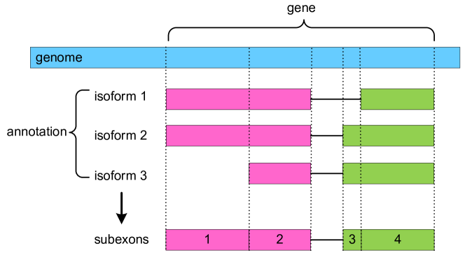
Due to the presence of numerous isoforms in existing annotations, inference on their abundance from RNA-seq reads has been an active field of research since 2009 (Jiang and Wong, 2009; Trapnell et al., 2010; Li et al., 2011; Zhang et al., 2014). A necessary step is to first map (or align) reads to reference genomes so that researchers know the numbers of reads generated from each exon. Then, a common approach to summarize RNA-seq reads is to categorize the reads by the genomic regions to which they map so that the number of reads in different genomic regions can be used to distinguish the abundance of various isoforms. As different isoforms may consist of overlapping but not identical exons, many methods divide exons into subexons, which are defined as transcribed regions between every two adjacent splicing sites in annotations (Li et al., 2011; Zhang et al., 2014; Ye and Li, 2016). By this definition, every gene is composed of non-overlapping subexons and introns (i.e., non-transcribed genomic regions). In Fig 1, we illustrate a toy example of a gene with three annotated isoforms and four subexons. Because combinations of subexons form a superset of all the annotated isoforms, it is reasonable to categorize RNA-seq reads based on the sets of subexons to which they map. For the ease of terminology, we will refer to subexons as exons for the remainder of this paper. For more details regarding categorizing RNA-seq reads, see Section 2.2.

Figure 1: Definition of subexons. The example gene has two exons, represented by magenta and green boxes, and three mRNA isoforms. The solid lines between exons represent introns in the gene that have been spliced out in isoforms. Adjacent splicing sites in these isoforms define four non-overlapping subexons: the first exon is divided into subexon 1 and 2, and the second exon is divided into subexon 3 and 4.

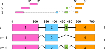
How to infer isoform abundance from observed RNA-seq reads is a statistical problem, as reads are generated from a mixture of isoforms. We illustrate this using a toy example in Fig 2. A hypothetical gene is composed of four non-overlapping exons. Suppose that the gene is transcribed into two mRNA isoforms: 60% of the transcripts are isoform 1, which consists of exons 1, 2 and 4, and 40% of the transcripts are isoform 2, which consists of all four exons. In reality, the isoform proportions, though of great interest to biologists, remain unobservable under the current experimental settings. Our aim is to estimate the relative abundance of annotated isoforms based on reads generated in RNA-seq experiments. Suppose that $n$ paired-end reads are generated from mRNA transcripts of the gene, and they are mapped (or aligned) to the reference genome. Some of the mapped reads have obvious isoform origins. For example, read $3$ is compatible only with isoform 2, and thus must have isoform 2 as its origin. On the other hand, many mapped reads can have ambiguous origins. For example, read 1 is compatible with both isoforms 1 and 2, and thus we cannot determine its origin isoform. The much more complex structures of real genes complicate the situation even further; human genes have nine exons on average (Sakharkar et al., 2004), and a large proportion of human genes have more than ten annotated isoforms (see Supplementary Fig S2B). Therefore, this problem requires powerful statistical methods to provide good estimates of isoform proportions.

Figure 2: Illustration of RNA-seq read generation from a hypothetical gene. The four exons of this gene are represented as boxes of different lengths and colors. The starting and ending positions of the four exons are marked on top of the gene. In an RNA-seq experiment, multiple reads are generated and the number of reads coming from each isoform is proportional to the isoform’s abundance. Each read has a 5’-end and a 3’-end, as shown in read 1. These reads are mapped to the reference genome and their overlapping exons are key information for estimating isoform abundance.

A number of isoform quantification methods have been developed to estimate the abundance of specific isoforms. These methods perform isoform quantification using either direct computation or model-based approaches (Wang et al., 2009; Steijger et al., 2013; Kanitz et al., 2015). Direct computation approaches use a variety of methods to count the number of reads compatible with each isoform and then normalize the counts by isoform lengths and the total number of reads to generate estimates of isoform abundance. The most commonly used unit is reads per kilobase of transcript per million mapped reads (RPKM) (Mortazavi et al., 2008). However, for complex gene structures, counts of RNA-seq reads compatible with isoforms may not be proportional to isoform abundance, as multiple isoforms can share exons and some reads cannot be assigned unequivocally to only one isoform. To address this issue, model-based approaches are needed to assess the likelihood of a read coming from different isoforms. In the first model-based isoform quantification method (Jiang and Wong, 2009), read counts in genomic regions are modeled as Poisson variables (with isoform abundance as the mean parameter), under the assumption that reads are uniformly sampled within each isoform. Isoform abundance is estimated by maximum likelihood estimates. Cufflinks (Trapnell et al., 2010), the most widely used method for discovering novel isoforms from RNA-seq data, also has the functionality to estimate isoform abundance. Its approach is similar to the likelihood-based approach in Jiang and Wong (2009), and it proposed a new unit for isoform abundance based on paired-end RNA-seq data: fragments per kilobase of transcript per million mapped reads (FPKM), which accounts for the dependency between paired-end reads. MISO (Katz et al., 2010) is another model-based method constructed under a Bayesian framework, and it provides maximum-a-posteriori estimates and confidence intervals of isoform abundance. There are other isoform quantification methods with different features (Pachter, 2011). For example, SLIDE (Li et al., 2011) uses a linear model and can be used with various data types; iReckon (Mezlini et al., 2013) utilizes a regularized Expectation-Maximization algorithm; WemIQ (Zhang et al., 2014) replaces the Poisson distribution with a more general and realistic generalized Poisson distribution; eXpress (Roberts and Pachter, 2013) is an efficient streaming method based on an online-EM algorithm and is considered to be a faster version of Cuffl inks with comparable performance; and Sailfish (Patro et al., 2014) is a fast alignment-free method that saves the read mapping step.

Figure 3: Reads in six hESC RNA-seq samples mapped to the human gene TPR. Detailed information on these samples is listed in Supplementary Table S2. The counts of RNA-seq reads are summarized in the histograms. The annotation of the gene and isoform structures is shown in the bottom row. We mark four example sites where the six samples are obviously inconsistent with red rectangles.

However, there remains much space to improve the accuracy of isoform quantification due to noise and biases in RNA-seq data. Because of the accumulation of RNA-seq samples in public databases, multiple RNA-seq data sets are now often available for the same biological condition (e.g., the same cell or tissue type), and they provide more information than a single RNA-seq data set. For example, the GTEx (Genotype-Tissue Expression) study comprises $9,662$ samples from $54$ tissues, and the Cancer Genome Atlas (TCGA) study comprises $11,350$ samples from $33$ cancer types (Collado-Torres et al., 2017). Here, the concept of multiple samples includes both technical replicates-different aliquots of the same sample measured multiple times (Hansen et al., 2011)- and biological replicates-replicates obtained from multiple samples of the same material, type of cells, or tissue. The availability of multiple RNA-seq samples from the same biological condition (e.g., human embryonic stem cells) in public databases (e.g., NIH Gene Expression Omnibus (Barrett et al., 2013)) motivated us to develop a new statistical method for better isoform quantification by taking advantage of the common and thus more reliable information provided by multiple samples. The necessity of such a method is two-fold. First, the number of RNA-seq samples produced by a single lab is limited since experimental costs increase each time an additional replicate is added. A statistical method that allows for multiple samples enables researchers to combine their own data with public data to obtain more accurate and robust isoform abundance estimates. Second, such a method supports better reuse of public data for both new biological findings and method development.

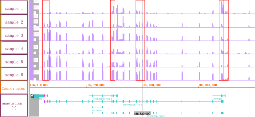
Several methods have been developed to use multiple RNA-seq samples from the same biological condition for isoform quantification. For example, CLIIQ (Lin et al., 2012) uses integer linear programming to jointly model RNA-seq data from multiple samples. MITIE (Behr et al., 2013) assumes that the same isoforms are expressed in all samples but may have different abundances, and it then reduces the problem to solving systems of linear equations. FlipFlop (Bernard et al., 2014) uses a convex formulation and introduces the group-lasso penalty to ensure sparsity in estimation. However, none of these methods considers the quality variation of different RNA-seq samples or how such variation might affect the inference of isoform abundance. It is commonly recognized that RNA-seq samples generated by different protocols or different labs can vary greatly with respect to the signal-to-noise ratios, biases, etc. For example, Fig 3 shows the RNA-seq read coverage profiles of the human gene TPR in six human embryonic stem cell (hESC) samples. There is obvious variation in the read coverage profiles of these six samples. For example, sample 2 has little signal in the last exon while the other samples have obviously stronger signals in the last exon. Thus, it is inappropriate to treat all the samples equally during isoform quantification by assuming that they come from the same population (i.e., the same tissue or cell of interest). Hence, results from these methods may be sensitive to the heterogeneity of samples or even, in some cases, be dominated by biased samples, which do not accurately reflect the transcriptome information of the given tissue type.

In this paper, we propose a robust quantification method for isoform expression: joint modeling of Multiple RNA-seq Samples for accurate Isoform Quantification (MSIQ). MSIQ is a model-based approach for estimating isoform abundance by discerning and using multiple RNA-seq samples that share similar transcriptome information, which we define as the consistent group in this paper. Our modeling consists of two components: (1) estimating the probability of each sample being in the consistent group via evaluating the sample similarities, and (2) estimating isoform abundance from reweighted samples, with greater weights given to the samples that are more likely to be consistent. These two components enable the method to distinguish between the large variation stemming from experimental factors and the reasonable biological variation. In Section 2, we describe the Bayesian hierarchical model used in MSIQ to bridge unknown isoform proportions and observed read counts mapped to a gene in multiple RNA-seq samples. Our model allows for different isoform proportions of RNA-seq samples inside and outside the consistent group; a main parameter of interest relates to the isoform proportions in the consistent group. This approach reduces the probability that the estimated isoform abundance is biased by samples of poor quality. We conduct parameter inference by Gibbs sampling and prove the consistency of the MSIQ estimator. We show that the isoform proportions estimated by MSIQ are consistent with the unknown isoform proportions in the consistent group, while the estimates based on the assumption that all samples have equal weights are not. In Section 3, we apply MSIQ to both simulated and real data sets to illustrate the efficiency and robustness of MSIQ under various parameter settings and with different parameter estimation procedures. We also compare MSIQ with the oracle estimators and other widely used estimation methods. In Section 4, we discuss the advantages and limitations of MSIQ and its possible extensions.

2 Methods

For a given gene, our proposed MSIQ method aims to achieve two goals with respect to isoform expression quantification. First, we want to identify the samples that represent the tissue or cell type of interest. We refer to these samples as the consistent group and assume that the group contains at least one sample. We identify samples in the consistent group under the assumption that these samples share the most similar read distributions among all the samples. Second, we would also like to estimate the proportion of reads coming from each mRNA isoform in the given tissue or cell type, with larger weights given to the samples in the consistent group. We focus our efforts on RNA-seq data with paired-end reads, but the model can easily be extended for single-end reads.

2.1 Ideal and practical parameters of interest

Suppose we are studying a gene with $N$ exons, $J$ annotated mRNA isoforms, and $D$ RNA-seq samples. Ideally, we are interested in the true proportion of each isoform

$$p_{j}=P(\text{an mRNA transcript is of isoform}\ j),\ j=1,2,...,J.$$

However, these hidden parameters are not observable in RNA-seq experiments, which do not directly measure full-length mRNA transcripts. Instead of directly estimating $p_{j}$, we aim to estimate the practical parameters

$$\alpha_{j}=P(\text{an RNA-seq read is from isoform}\ j),\ j=1,2,...,J,$$

which we refer to as isoform proportions in our discussion.

2.2 Observed data

We denote the observed data, $D$ independent samples of reads mapped to the given gene, by

$$\bm{R}^{(d)}=\{r^{(d)}_{1},r^{(d)}_{2},\dots,r^{(d)}_{n_{d}}\}\,,\quad d=1\,,2\,,\dots,D\,,$$

where $n_{d}$ and $r^{(d)}_{i}$, respectively, denote the total number of reads and the $i$th read ($i=1,2,\dots,n_{d}$) in sample $d$. To use the read information, an efficient data summary is needed to preserve the most relevant information for isoform quantification while limiting the computational complexity to a manageable level (Rossell et al., 2014). We write each read as

$$r^{(d)}_{i}=\left\{\bm{s}^{(d)}_{1i},\bm{s}^{(d)}_{2i},\left\{y_{i1}^{(d)},y_{ic^{(d)}}^{(d)},y_{i(c^{(d)}+1)}^{(d)},y_{i(2c^{(d)})}^{(d)}\right\}\right\},$$

where $\bm{s}^{(d)}_{1i}\ \text{and}\ \bm{s}^{(d)}_{2i}$, respectively, denote the index set of exons overlapping with the read’s left end and right end; $y_{ik}^{(d)}$ denotes the $k$th genomic position of read $i$; and $c^{(d)}$ is the read length in sample $d$. Please refer to the supplementary information for a more detailed discussion on the advantages of this summarizing approach over other existing approaches.

2.3 Assumptions and prior

In addition to the observed data, we consider the hidden data, which are the isoform origins of the reads:

$$\bm{Z}^{(d)} = (Z^{(d)}_{1},Z^{(d)}_{2},\dots,Z^{(d)}_{n_{d}})^{\prime}\,,$$

where $Z^{(d)}_{i}\in\{1,2,\dots,J\}$ indicates the isoform origin of read $i$, and $Z^{(d)}_{i}=j$ if read $r^{(d)}_{i}$ actually comes from isoform $j$.

The differences between RNA-seq samples are reflected in their isoform proportion $\bm{\tau}^{(d)}$, $d=1,2,\dots,D$. In RNA-seq sample $d$, we denote the true probability of reads from isoform $j$ as $\tau^{(d)}_{j}=P(Z^{(d)}_{i}=j)$ and the isoform proportion vector as

$$\bm{\tau}^{(d)}=(\tau^{(d)}_{1},\tau^{(d)}_{2},\dots,\tau^{(d)}_{J})^{\prime}\,,$$

with $\sum^{J}_{j=1}\tau^{(d)}_{j}=1$. We define a hidden state variable $E_{d}$ for each sample such that

$$E_{d}={\rm 1}\kern-2.40005pt{\rm I}\{\text{sample $d$ belongs to the consistent group}\}.$$

We assume samples in the consistent group all have the same proportion vector $\bm{\alpha}=(\alpha_{1},\alpha_{2},\dots,\alpha_{J})^{\prime}\ \text{with}\ \sum^{J}_{j=1}\alpha_{j}=1$, while samples not in the consistent group can each have different isoform proportions $\bm{\beta}^{(d)}=(\beta_{1}^{(d)},\beta_{2}^{(d)},\dots,\beta_{J}^{(d)})^{\prime}$ $\sum^{J}_{j=1}\beta_{j}^{(d)}=1$. Thus the isoform proportions can be expressed as

$$\bm{\tau}^{(d)} = E_{d}\cdot{\bm{\alpha}}+(1-E_{d})\cdot{\bm{\beta}}^{(d)}$$

$$= \left\{\begin{array}[]{ll}\bm{\alpha},&\text{if}\ E_{d}=1\,,\\ {\bm{\beta}}^{(d)},&\text{if}\ E_{d}=0\,.\end{array}\right.$$

The isoform proportion vector of the consistent group $\alpha$ is our parameter of interest.

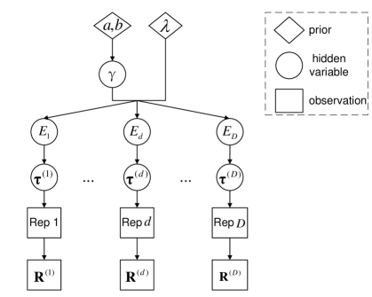
We assume $\bm{\alpha}$ and $\bm{\beta}^{(d)}$ are a priori $\text{Dirichlet}(\bm{\lambda})$, and $E_{d}$ is a priori $\text{Bernoulli}(\gamma)$: $E_{d}|\gamma\sim\text{Bernoulli}(\gamma),\text{where}\ \gamma\sim\text{Beta}(a,b).$ Intuitively, $\bm{\lambda}$ controls the distance between the isoform proportions of samples inside and outside the consistent group, while $\gamma$ controls the tendency of assigning a sample to the consistent group. We describe the relationship between observed RNA-seq reads and hidden isoform proportions in multiple samples under a Bayesian framework (Fig 4).

Figure 4: Joint modeling of multiple RNA-seq samples. In this framework, $E_{d}\ (d=1,2,\dots,D)$ is a binary hidden state variable indicating whether RNA-seq sample $d$ is in the consistent group, while $a,b$ and $\gamma$ are hyper-parameters (priors) in $E_{d}$’s distribution. Depending on $E_{d}$, the isoform proportion vector $\bm{\tau}^{(d)}$ takes either the consistent group’s isoform proportion vector $\bm{\alpha}$ or its own $\bm{\beta}^{(d)}$. Given the isoform proportions, RNA-seq reads are generated in each sample, and our observed data are summarized as $\bm{R}^{(d)}$ (see Section 2.2).

2.4 The MSIQ model

We introduce $I^{(d)}_{i,j}$ as a short notation of binary variable ${\rm 1}\kern-2.40005pt{\rm I}\{Z^{(d)}_{i}=j\}$. Then given a sample with isoform proportion $\bm{\tau}^{(d)}$, the probability of read $r^{(d)}_{i}$ and origin $Z^{(d)}_{i}$ can be written as follows:

$$P\left(r^{(d)}_{i},Z^{(d)}_{i}|\bm{\tau}^{(d)}\right) = \prod_{j=1}^{J}P\left(r^{(d)}_{i},Z^{(d)}_{i}=j|\bm{\tau}^{(d)}\right)^{{\rm 1}\kern-1.68004pt{\rm I}\{Z^{(d)}_{i}=j\}}$$ (2.2)

$$= \prod_{j=1}^{J}\left[P\left(r^{(d)}_{i}|Z^{(d)}_{i}=j\right)\tau^{(d)}_{j}\right]^{I^{(d)}_{i,j}}\triangleq\prod_{j=1}^{J}\left(h_{i,j}^{(d)}\tau^{(d)}_{j}\right)^{I^{(d)}_{i,j}},$$

where $P\left(r^{(d)}_{i},Z^{(d)}_{i}|\bm{\tau}^{(d)}\right)$ refers to the joint density of read $r_{i}^{(d)}$ and its isoform origin $Z_{i}^{(d)}$ given the model parameters, and $h_{i,j}^{(d)}$ is the generating probability of read $r_{i}^{(d)}$ given isoform $j$. If read $r_{i}^{(d)}$ and isoform $j$ are incompatible (e.g., read 2 in Fig 2 cannot come from isoform 1), $h_{i,j}^{(d)}=0$. Otherwise, $h_{i,j}^{(d)}$ depends on the model for the read generation mechanism. We adopt the following model from Zhang et al. (2014):

$$h_{i,j}^{(d)}=\frac{1}{\ell^{\prime}_{j}}\times P\left(L^{(d)}_{i,j}\right),$$

where $\ell^{\prime}_{j}$ is the effective length (i.e., the number of possible starting positions on the fragment) of isoform $j$ and can be calculated as $\ell^{\prime}_{j}=\ell_{j}-L^{(d)}$: $\ell_{j}$ is the length of isoform $j$ and $L^{(d)}$ is the mean fragment length in sample $d$. $L^{(d)}_{i,j}$ denotes the fragment length of $r^{(d)}_{i}$ if it comes from isoform $j$. Note that the same read may correspond to different fragment lengths if they come from different isoforms. For example, read 1 in Fig 2 corresponds to fragments of different lengths in isoforms 1 and 2. $L^{(d)}_{i,j}$ is assumed to be a Gaussian random variable and its mean $L^{(d)}=\mathbb{E}({L^{(d)}_{i,j}})$ and variance $\text{var}({L^{(d)}_{i,j}})$ can be estimated from single-isoform genes, whose mapped reads directly determine fragment lengths.

Let $\bm{E}=(E_{1},E_{2},\dots,E_{D})^{\prime}$ be the hidden state vector indicating whether each sample is among the consistent group or not, and let $\bm{R}=\{\bm{R}^{(d)}\}_{d=1}^{D}$, $\bm{Z}=\{\bm{Z}^{(d)}\}_{d=1}^{D}$, and $\bm{\bm{\tau}}=\{{\bm{\tau}}^{(d)}\}_{d=1}^{D}$ represent the reads, origins of reads, and isoform proportions in all the samples, respectively. To simplify the notation, we also introduce $n^{(d)}_{j}=\sum_{i=1}^{n_{d}}I^{(d)}_{i,j}$ to represent the total number of reads coming from isoform $j$ in sample $d$. Given equation (2.2), the joint probability of all reads in the MSIQ model is as follows:

$$P\left(\bm{R},\bm{Z},\bm{\tau},\bm{E},\gamma|\bm{\lambda},a,b\right)=P\left(\left.\bm{R},\bm{Z}\right|\bm{\tau},\bm{E}\right)P\left(\left.\bm{\tau}\right|\bm{\lambda},\bm{E}\right)P\left(\left.\bm{E}\right|\gamma\right)P(\gamma|a,b)\,,$$

where

$$P\left(\left.\bm{R},\bm{Z}\right|\bm{\tau},\bm{E}\right) = \prod_{d=1}^{D}\left\{\left[\prod_{i=1}^{n_{d}}\prod_{j=1}^{J}\left(h_{i,j}^{(d)}\alpha_{j}\right)^{I^{(d)}_{i,j}}\right]^{E_{d}}\left[\prod_{i=1}^{n_{d}}\prod_{j=1}^{J}\left(h_{i,j}^{(d)}\beta^{(d)}_{j}\right)^{I^{(d)}_{i,j}}\right]^{1-E_{d}}\right\},$$

$$P\left(\left.\bm{\tau}\right|\bm{\lambda},\bm{E}\right) \propto \prod_{j=1}^{J}\alpha_{j}^{\lambda_{j}-1}\prod_{d=1}^{D}\left[\prod_{j=1}^{J}\left(\beta^{(d)}_{j}\right)^{\lambda_{j}-1}\right]^{1-E_{d}}\,,$$

$$P\left(\left.\bm{E}\right|\gamma\right) \propto \gamma^{\sum^{D}_{d=1}E_{d}}(1-\gamma)^{D-\sum^{D}_{d=1}E_{d}}\,,$$

$$P(\gamma|a,b) \propto \gamma^{a-1}(1-\gamma)^{b-1}\,.$$

As a result, the joint probability can be simplified as

$$P\left(\bm{R},\bm{Z},\bm{\tau},\bm{E},\gamma|\bm{\lambda},a,b\right)$$

$$\propto \left[\prod_{j=1}^{J}\alpha_{j}^{\lambda_{j}-1+\sum_{d=1}^{D}E_{d}n^{(d)}_{j}}\right]\left[\prod^{D}_{d=1}\prod^{J}_{j=1}\left(\beta_{j}^{(d)}\right)^{(1-E_{d})\left(\lambda_{j}-1+n^{(d)}_{j}\right)}\right]$$

$$\left[\prod^{D}_{d=1}\prod^{J}_{j=1}\prod^{n_{d}}_{i=1}\left(h_{i,j}^{(d)}\right)^{I^{(d)}_{i,j}}\right]\gamma^{\sum^{D}_{d=1}E_{d}+a-1}(1-\gamma)^{D-\sum^{D}_{d=1}E_{d}+b-1}\,.$$

2.5 Markov chain Monte Carlo

In the MSIQ model (2.4), the reads $\bm{R}$ are the observed data, the isoform origins $\bm{Z}$ and the consistent group indicator $\bm{E}$ are the hidden data, while isoform proportions $\bm{\alpha},\{\bm{\beta}^{(d)}\}^{D}_{d=1}$, and consistent group proportion $\gamma$ are the parameters. To estimate the parameters, a useful approach is to implement a Gibbs sampler to iteratively draw posterior samples of hidden data and parameters from their conditional distributions. Since our ultimate parameter of interest is $\bm{\alpha}$, whose inference becomes obvious given $\bm{Z}$ and $\bm{E}$, we integrate out $\bm{\bm{\tau}}$ (i.e., $\bm{\alpha}$ and $\{\bm{\beta}^{(d)}\}^{D}_{d=1}$) in model (2.4) to achieve better computational efficiency. This step is based on a property of the Dirichlet distribution:

$$\int\cdots\int_{\{(\tau_{1},\ldots,\tau_{J}):0\leq\tau_{j}\leq 1,\sum_{j}\tau_{j}=1\}}\prod_{j=1}^{J}\tau_{j}^{\lambda_{j}-1}d\tau_{1}\cdots d\tau_{J}=B(\bm{\lambda}),\quad\forall\lambda_{j}>0\,,$$

where $B(\bm{\lambda})=\frac{\Pi^{J}_{j=1}\Gamma(\lambda_{j})}{\Gamma(\sum^{J}_{j=1}\lambda_{j})}$. Hence,

$$P\left(\left.\bm{R},\bm{Z},\bm{E},\gamma\right|\bm{\lambda},a,b\right) \propto B_{1}(\bm{Z},\bm{E})\cdot\prod_{d=1}^{D}B_{0}^{(d)}(\bm{Z}^{(d)},E_{d})\cdot\left[\prod_{d=1}^{D}\prod_{i=1}^{n_{d}}\prod_{j=1}^{J}\left(h_{i,j}^{(d)}\right)^{I^{(d)}_{i,j}}\right]$$

$$\cdot\gamma^{\sum^{D}_{d=1}E_{d}+a-1}(1-\gamma)^{D-\sum^{D}_{d=1}E_{d}+b-1}\,,$$

where

$$B_{1}(\bm{Z},\bm{E}) = \frac{\prod_{j=1}^{J}\Gamma\left(\lambda_{j}+\sum_{d=1}^{D}E_{d}\cdot n^{(d)}_{j}\right)}{\Gamma\left(\sum_{j=1}^{J}\lambda_{j}+\sum_{d=1}^{D}E_{d}\cdot n_{d}\right)}\,,$$

$$B_{0}^{(d)}(\bm{Z}^{(d)},E_{d}=1) = 1,$$

$$B_{0}^{(d)}(\bm{Z}^{(d)},E_{d}=0) = \frac{\prod_{j=1}^{J}\Gamma\left(\lambda_{j}+n^{(d)}_{j}\right)}{\Gamma\left(\sum_{j=1}^{J}\lambda_{j}+n_{d}\right)}\,.$$

We denote $\Theta=\{\bm{Z},\bm{E},\gamma\}$. The distribution of each parameter or hidden variable conditional on everything else can thus be estimated by Gibbs sampling as follows.

• $E_{d}$ follows a Bernoulli distribution:

  $$E_{d}|\Theta/\{E_{d}\} \sim \text{Bern}\left(\frac{odds(E_{d};\bm{\lambda},\tau)}{1+odds(E_{d};\bm{\lambda},\tau)}\right)\,,$$ (2.4)

  where

  $$odds(E_{d};\bm{\lambda},\tau) = \frac{P(E_{d}=1|\Theta/\{E_{d}\})}{P(E_{d}=0|\Theta/\{E_{d}\})}=\frac{P\left(\left.\bm{R},\bm{Z},\bm{E}_{-d},E_{d}=1,\gamma\right|\bm{\lambda},a,b\right)}{P\left(\left.\bm{R},\bm{Z},\bm{E}_{-d},E_{d}=0,\gamma\right|\bm{\lambda},a,b\right)}$$

  $$= \frac{B_{1}(\bm{Z},\bm{E}_{-d},E_{d}=1)}{B_{1}(\bm{Z},\bm{E}_{-d},E_{d}=0)}\cdot\frac{B_{0}^{(d)}(\bm{Z}^{(d)},E_{d}=1)}{B_{0}^{(d)}(\bm{Z}^{(d)},E_{d}=0)}\cdot\frac{\gamma}{1-\gamma}\,.$$

• $Z^{(d)}_{i}$ follows a multinomial distribution:

  $$Z^{(d)}_{i}|\Theta/\{Z^{(d)}_{i}\} \sim \text{Multinomial}\left(q^{(d)}_{i,1},q^{(d)}_{i,2},\dots,q^{(d)}_{i,J}\right)\,,$$ (2.5)

  where

  $$q^{(d)}_{i,j} = \frac{P(Z^{(d)}_{i}=j|\Theta/\{Z^{(d)}_{i}\})}{\sum^{J}_{j^{\prime}=1}P(Z^{(d)}_{i}=j^{\prime}|\Theta/\{Z^{(d)}_{i}\})}=\frac{P\left(\left.\bm{R},\bm{Z}^{(-d)}_{-i},Z^{(d)}_{i}=j,\bm{E},\gamma\right|\bm{\lambda},a,b\right)}{\sum^{J}_{j^{\prime}=1}P\left(\left.\bm{R},\bm{Z}^{(-d)}_{-i},Z^{(d)}_{i}=j^{\prime},\bm{E},\gamma\right|\bm{\lambda},a,b\right)}\,.$$

• $\gamma$ follows a Beta distribution:

  $$\gamma|\Theta/\{\gamma\}\sim\text{Beta}\left(\sum_{d=1}^{D}E_{d}+a,D-\sum_{d=1}^{D}E_{d}+b\right)\,.$$ (2.6)

2.6 Estimators of isoform proportions

With the above posterior distribution of the hidden variables and parameters, we can draw samples iteratively to estimate the hidden state of each RNA-seq sample and the true isoform proportions in the consistent group. Suppose we have $T$ iterations available after discarding the burn-in period of Gibbs sampling. In each iteration, we denote the sampled hidden state vector as $\bm{E}^{(t)}=(E^{(1)}_{1},E^{(2)}_{2},\dots,E^{(T)}_{D})^{\prime}$ and the hidden origin vector in sample $d$ as $(Z^{(d,t)}_{1},\dots,Z^{(d,t)}_{n_{d}})^{\prime}$.

To estimate isoform proportions in each iteration, we pool the reads from sample $d$ whose state varibale $E^{(t)}_{d}=1$ to calculate $\bm{\alpha}^{(t)}$, where

$$\bm{\alpha}_{j}^{(t)}=\frac{\lambda_{j}+\sum^{D}_{d=1}\left(E_{d}^{(t)}\sum^{n_{d}}_{i=1}{\rm 1}\kern-2.40005pt{\rm I}\{Z^{(d,t)}_{i}=j\}\right)}{\sum^{J}_{j=1}\lambda_{j}+\sum^{D}_{d=1}E_{d}^{(t)}n_{d}}.$$ (2.7)

Overall, the MSIQ estimator of the isoform proportions becomes

$$\hat{\bm{\alpha}}^{\text{MSIQ}}=\frac{1}{T}\sum_{t=1}^{T}\bm{\alpha}^{(t)},$$

and the relative estimation error is calculated as

$$\text{REE}(\hat{\bm{\alpha}}^{\text{MSIQ}})=\sum^{m}_{j=1}|\alpha_{j}-\hat{\bm{\alpha}}_{j}^{\text{MSIQ}}|/\alpha_{j}.$$

We prove the consistency property of the MSIQ estimator $\hat{\bm{\alpha}}^{MSIQ}$ in the following lemma. (Please refer to the supplementary information for the complete proof.)

Lemma 2.1.

$\hat{\bm{\alpha}}^{\text{MSIQ}}$ converges to the posterior mean of isoform proportion $\mathbb{E}(\bm{\alpha}|\bm{R},\bm{\lambda},a,b)$:

$$\lim_{T\to\infty}\hat{\bm{\alpha}}^{\text{MSIQ}}=\mathbb{E}(\bm{\alpha}|\bm{R},\lambda,a,b).$$

We can also estimate the posterior probability of each sample belonging to the consistent group: $\bm{\theta}=(\theta_{1},\theta_{2},\dots,\theta_{D})^{\prime}$, where $\theta_{d}=P(E_{d}=1|\bm{R},\bm{\lambda},a,b)$, and the estimator is

$$\hat{\theta}_{d}^{\text{MSIQ}}=\frac{1}{T}\sum_{t=1}^{T}E^{(t)}_{d}.$$

Based on this posterior probability, we predict the state variable of each sample: $\hat{E}_{d}={\rm 1}\kern-2.40005pt{\rm I}\{\hat{\theta}_{d}^{\text{MSIQ}}>1/2\}$.

To further evaluate the biological variation within the consistent group, we estimate the standard error of the MSIQ estimator given the posterior samples drawn by the Gibbs sampling. For isoform $j$, the standard error of the respective entry in $\hat{\bm{\alpha}}^{\text{MSIQ}}$ is estimated as:

$$\hat{\sigma}_{j}=\sqrt{\frac{1}{T}\sum^{T}_{t=1}(\bm{\alpha}_{j}^{(t)}-\hat{\bm{\alpha}}_{j}^{\text{MSIQ}})^{2}}\,.$$ (2.8)

Note that the consistent group is automatically selected by the MSIQ model given the overall heterogeneity among samples. Even though the consistent group is assumed to have a consensus isoform proportion, it is useful to account for the biological variation, especially when the overall heterogeneity is non-negligible.

We also consider six competing estimators to demonstrate the effectiveness of MSIQ in accurate isoform quantification. From what has been derived in Section 2.4, we know that the log likelihood of all reads in sample $d$ is

$$\log\left(P(\bm{R}^{(d)},\bm{Z}^{(d)}|\bm{\tau}^{(d)})\right) = \sum_{i=1}^{n_{d}}\sum_{j=1}^{m}I^{(d)}_{i,j}\log\left(h^{(d)}_{i,j}\tau^{(d)}_{j}\right).$$

Then the EM algorithm can be implemented to estimate $\bm{\tau}^{(d)}$ by maximizing the log likelihood. The six competing estimators are calculated using the EM algorithm based on different sets of samples:

AVG (averaging): We calculate the isoform proportion in each sample and take the average of them as the estimator of isoform proportion,

$$\hat{\bm{\alpha}}^{\text{AVG}}=\frac{1}{D}\sum^{D}_{d=1}\hat{\bm{\tau}}^{(d)}.$$

AVG* (oracle averaging): We calculate the isoform proportion in each sample in the true consistent group and take the average of them as the estimator of isoform proportion,

$$\hat{\bm{\alpha}}^{\text{AVG*}}=\frac{\sum^{D}_{d=1}\hat{\bm{\tau}}^{(d)}{\rm 1}\kern-2.40005pt{\rm I}\{E_{d}=1\}}{\sum^{D}_{d=1}{\rm 1}\kern-2.40005pt{\rm I}\{E_{d}=1\}}.$$

POOL (pooling): We pool the reads in all samples together, then we use the EM algorithm to estimate the isoform proportion $\bm{\tau}$ as $\hat{\bm{\alpha}}^{\text{POOL}}$.

POOL* (oracle pooling): We pool the reads in samples in the true consistent group together, then we use the EM algorithm to estimate $\bm{\tau}$ as $\hat{\bm{\alpha}}^{\text{POOL*}}$.

MSIQa (MSIQ averaging): We calculate the isoform proportion in each sample in the consistent group (identified by MSIQ) and take the average of them as the estimator of isoform proportion,

$$\hat{\bm{\alpha}}^{\text{MSIQa}}=\frac{\sum^{D}_{d=1}\hat{\bm{\tau}}^{(d)}{\rm 1}\kern-2.40005pt{\rm I}\{\hat{\theta}_{d}^{\text{MSIQ}}>1/2\}}{\sum^{D}_{d=1}{\rm 1}\kern-2.40005pt{\rm I}\{\hat{\theta}_{d}^{\text{MSIQ}}>1/2\}}.$$

MSIQp (MSIQ pooling): We pool the reads of the given gene in the samples in the consistent group (identified by MSIQ) together, then we use the EM algorithm to estimate $\bm{\tau}$ as $\hat{\bm{\alpha}}^{\text{MSIQp}}$.

Among these estimators, $\hat{\bm{\alpha}}^{\text{AVG*}}$ and $\hat{\bm{\alpha}}^{\text{POOL*}}$ are oracle estimators that we take as gold standards in simulations but are unknown in real data; $\hat{\bm{\alpha}}^{\text{MSIQa}}$ and $\hat{\bm{\alpha}}^{\text{MSIQp}}$ are MSIQ-dependent and rely on $\hat{\bm{\theta}}$ estimated by MSIQ.

3 Results

3.1 Performance of MSIQ in simulations

To show that MSIQ provides more accurate estimates of isoform expression than the current averaging or pooling method, we compare the relative estimation errors (REE) of $\hat{\bm{\alpha}}^{\text{MSIQ}}$ with those of the six competing estimators: $\hat{\bm{\alpha}}^{\text{AVG*}}$, $\hat{\bm{\alpha}}^{\text{MSIQa}}$, $\hat{\bm{\alpha}}^{\text{AVG}}$, $\hat{\bm{\alpha}}^{\text{POOL*}}$, $\hat{\bm{\alpha}}^{\text{MSIQp}}$, and $\hat{\bm{\alpha}}^{\text{POOL}}$. It is difficult to compare these methods on real data because true isoform abundances in samples are unknown. Although the quantitative polymerase chain reaction (qPCR) technology can accurately measure the abundance of mRNA isoforms and produce “gold standard” isoform abundance, qPCR data sets are scarce and unavailable for most biological conditions (Li and Dewey, 2011). We use simulated data to compare the performances of these estimators under various scenarios and parameter settings.

Table 1: Four parameter settings and five scenarios in the simulation study.

setting	average fragment length (bp)	read length (bp)
1	150	50
2	250	50
3	150	100
4	250	100
scenario	% samples in the consistent group	isoform proportions
1	100	$\{\bm{\alpha},\bm{\alpha},\bm{\alpha},\bm{\alpha},\bm{\alpha},\bm{\alpha},\bm{\alpha},\bm{\alpha},\bm{\alpha},\bm{\alpha}\}$
2	50	$\{\bm{\alpha},\bm{\alpha},\bm{\alpha},\bm{\alpha},\bm{\alpha},\bm{\beta}_{1},\bm{\beta}_{2},\bm{\beta}_{3},\bm{\beta}_{4},\bm{\beta}_{5}\}$
3	70	$\{\bm{\alpha},\bm{\alpha},\bm{\alpha},\bm{\alpha},\bm{\alpha},\bm{\alpha},\bm{\alpha},\bm{\beta}_{1},\bm{\beta}_{2},\bm{\beta}_{3}\}$
4	70	$\{\bm{\alpha},\bm{\alpha},\bm{\alpha},\bm{\alpha},\bm{\alpha},\bm{\alpha},\bm{\alpha},\bm{\beta}_{6},\bm{\beta}_{6},\bm{\beta}_{6}\}$
5	70	$\{\bm{\alpha},\bm{\alpha},\bm{\alpha},\bm{\alpha},\bm{\alpha},\bm{\alpha},\bm{\alpha},\bm{\beta}_{7},\bm{\beta}_{7},\bm{\beta}_{7}\}$

We simulate RNA-seq reads from $3,421$ D.melanogaster (fly) genes that have multiple isoforms in the annotation (September 2010) available in the UCSC Genome Browser. Among these genes, $221$ have $3$ exons, $330$ have $4$ exons, $365$ have $5$ exons, $370$ have $6$ exons, $320$ have $7$ exons, $311$ have $8$ exons, $256$ have $9$ exons, $292$ have $10$ exons, and $956$ genes have more than 10 exons. The isoform numbers increase at a roughly exponential rate as the exon numbers increase (see Supplementary Fig S2A). We simulate ten samples and $500$ paired-end reads from each gene in every sample. To fully evaluate the performances of the seven estimators, we consider five different scenarios with different numbers of samples in the consistent group.

For each gene, we first independently generate the isoform proportion vector $\bm{\alpha}$ for the samples in the consistent group and the isoform proportion vectors $\bm{\beta}_{1},\bm{\beta}_{2},\bm{\beta}_{3},\bm{\beta}_{4}\,\text{and}\ \bm{\beta}_{5}$ for the other five samples. The five scenarios are designed as follows (see Table 1).

• In scenario 1, all ten samples are in the consistent group.

• In scenario 2, five samples are in the consistent group, and the other five samples have individual isoform proportions $\bm{\beta}_{1},\bm{\beta}_{2},\bm{\beta}_{3},\bm{\beta}_{4}\ \text{and}\ \bm{\beta}_{5}$.

• In scenario 3, seven samples are in the consistent group, and the other three samples have individual isoform proportions $\bm{\beta}_{1},\bm{\beta}_{2}\ \text{and}\ \bm{\beta}_{3}$.

• In scenario 4, seven samples are in the consistent group, and the other three samples have the same isoform proportion vector as

  $$\bm{\beta}_{6}=\operatorname*{arg\!max}\limits_{\bm{\beta}_{i},i=1,\ldots,5}||\bm{\beta}_{i}-\bm{\alpha}||_{2}^{2}\,,$$

  which is the isoform proportion vector most different from $\bm{\alpha}$.

• In scenario 5, seven samples are in the consistent group, and the other three samples have the same isoform proportion vector as

  $$\bm{\beta}_{7}=\operatorname*{arg\!min}\limits_{\bm{\beta}_{i},i=1,\ldots,5}||\bm{\beta}_{i}-\bm{\alpha}||_{2}^{2}\,,$$

  which is the isoform proportion vector most similar to $\bm{\alpha}$.

We also consider four settings of fragment and read length (Table 1) to examine how these parameters affect the performances of the seven estimators on isoform quantification. Under each setting, we first determine the origin of a fragment according to the designated isoform proportion, and then the starting position and the fragment length can be simulated from a uniform distribution and a normal distribution, respectively (with a standard deviation of $10$ bp). Once the starting and ending positions of the fragments are determined, the corresponding paired-end reads are also obtained.

For each scenario and parameter setting, we calculate the seven estimators, and then evaluate their estimation accuracy by calculating the REE of these estimates against the true isoform proportions. When calculating $\hat{\bm{\alpha}}^{\text{MSIQ}}$, we set the hyper-parameters in model (2.4) as $a=7$ and $b=2$. We have also included a sensitivity analysis of the MSIQ method on these two parameters in the supplementary information.

Figure 5: Relative estimation error (REE) rates of the seven estimators in scenarios 1-5. REE rates are calculated on 2,465 fly genes with 3-10 exons. In each boxplot, the REE rates of MSIQ, AVG^∗ (oracle averaging), MSIQa, AVG (averaging), POOL^∗ (oracle pooling), MSIQp and POOL (pooling) are plotted side by side under each scenario and the whiskers extend to the most extreme REE rates. The top-right legend of each plot displays the parameter setting: the mean fragment length (F) and the read length (R).

3.1.1 MSIQ achieves the lowest error rates in different scenarios

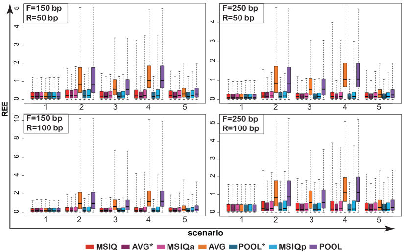
We calculate the error rates of the seven estimators for the $2,465$ fly genes with no more than ten exons in different scenarios and parameter settings, and illustrate the results in Fig 5. The results suggest that given the samples not in the consistent group (scenarios 2-5), especially when these samples constitute a large proportion or are vastly different from the consistent group, MSIQ ($\hat{\bm{\alpha}}^{\text{MSIQ}}$) and MSIQ-based methods ($\hat{\bm{\alpha}}^{\text{MSIQa}}$ and $\hat{\bm{\alpha}}^{\text{MSIQp}}$) achieve much smaller error rates than the averaging or pooling methods ($\hat{\bm{\alpha}}^{\text{AVG}}$ and $\hat{\bm{\alpha}}^{\text{POOL}}$). Compared with $\hat{\bm{\alpha}}^{\text{MSIQ}}$, $\hat{\bm{\alpha}}^{\text{AVG}}$ results in a $17.3$-fold increase in the REE rates on average, and $\hat{\bm{\alpha}}^{\text{POOL}}$ results in a $17.6$-fold increase. We also summarize the REE of the seven estimators (see Fig A1 in the Appendix) when we include the $956$ fly genes with more than ten exons. The isoform quantification task is much more challenging for these $956$ genes since they have many more annotated isoforms (see Supplementary Fig S2A). As expected, both the largest and the average REE rates increase with the addition of these 956 genes, because their complicated isoform structures introduce more difficulty and complexity in model fitting and computation. These results suggest that, compared with the direct averaging or pooling method, the MSIQ methods, which take the quality of samples into consideration, can lead to more accurate isoform quantification when multiple RNA-seq samples are available. Fig 5 also shows that MSIQ can constrain the estimation error to a much narrower range compared with direct averaging and pooling. MSIQ is able to control the REE rate below $1.33$ for 90% of the $2,465$ genes, while direct averaging and pooling give rise to REE rates larger than $2.00$ for more than 15% of these genes. We conclude that MSIQ is a more robust method than direct averaging and pooling.

Table 2: Median REE rates of five estimators under the five scenarios. The values are averaged over the four parameter settings and rounded to three decimal places. Differences in REE rates between MSIQ and the four other estimators are listed in parentheses.

estimator	scenario 1	scenario 2	scenario 3	scenario 4	scenario 5
MSIQ	0.157	0.236	0.194	0.208	0.211
AVG*	0.158	0.215	0.179	0.179	0.179
	(-0.001)	(0.021)	(0.014)	(0.029)	(0.031)
MSIQa	0.164	0.244	0.202	0.222	0.217
	(-0.007)	(-0.009)	(-0.009)	(-0.014)	(-0.006)
POOL*	0.152	0.212	0.175	0.175	0.175
	(0.005)	(0.023)	(0.019)	(0.033)	(0.036)
MSIQp	0.157	0.242	0.200	0.217	0.215
	(-0.000)	(-0.006)	(-0.007)	(-0.009)	(-0.005)

Figure 6: Median REE rates of the MSIQ-based and oracle estimators in scenarios 1-5. MSIQ outperforms MSIQa and MSIQp and gives error rates close to those of the oracle estimators. The parameter setting: the mean fragment length (F) and the read length (R) are listed on the top of each panel. The standard errors of MSIQ’s REE rates are given under each scenario. The smallest standard error in each scenario is marked in red.

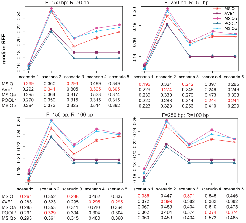
We also summarize the median REE of these estimators under different scenarios in Fig 6 and Table 2. The results show that MSIQ not only outperforms direct averaging and pooling, as we have seen, but also achieves more accurate abundance estimation than MSIQa and MSIQp. Compared with MSIQ’s median REE rate, MSIQa and MSIQp have average REE rates that are greater by 0.009 and 0.007, respectively. From Fig 6 and Table 2 we also conclude that the estimation results of MSIQ are similar to those of AVG^∗ and POOL^∗, the two oracle estimators that are impossible to calculate on real data. On average, the REE rate of MSIQ is only 0.019 larger than AVG^∗ and 0.058 larger than POOL^∗.

3.1.2 Different scenarios influence estimators’ performance

Since AVG and POOL are observed to have much poorer accuracy than the other five estimation methods, we remove them from the comparison for a more detailed evaluation of the other five methods. From Fig 6, it is obvious that the proportion of samples in the consistent group and the difference between the consistent group and other samples have large effects on the performances of all five estimating methods: MSIQ, AVG*, MISQa, POOL*, and MISQp. In scenario 1 when all the samples are in the consistent group, the five methods exhibit their lowest median REE rates for the $2,465$ genes. In scenario 2, which has the smallest proportion of samples in the consistent group, all five methods have the largest median REE rates among all scenarios. This phenomenon can be explained by the fact that having fewer samples in the consistent group leads to more error-prone identification of these samples and less accurate estimates of the isoform proportions. In scenarios 3, 4, and 5, in which 70% of the samples are in the consistent group, the REE rates of the five methods lie between those of scenarios 1 and 2. Among all three non-oracle estimation methods (MSIQ, MSIQa and MSIQp), MSIQ has the best performance in all five scenarios. Unlike MSIQa and MSIQp, which discard the samples outside of the identified consistent group, MSIQ partially borrows information from these samples through the Bayesian hierarchical framework.

Figure 7: REE rates of MSIQ for RNA-seq samples with different fragments and read lengths. The median, the 1st quartile and the 3rd quartile of the REE rates in different scenarios are illustrated in the boxplots, respectively. The top left legend of each plot displays the parameter setting: the mean fragment length (F) and the read length (R).

3.1.3 More accurate isoform quantification with longer fragments

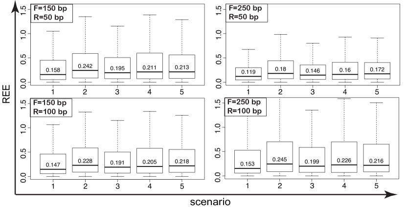
We also evaluate the REE rates of MSIQ with different fragment lengths and read lengths in simulated RNA-seq experiments. The 1st quartile, median, and 3rd quartile of the REE errors in each of the five scenarios are illustrated in Fig 7. It is obvious that longer fragment lengths would improve the estimation accuracy, especially when read lengths are short. Specifically, when read lengths are set to 50 bp, increasing fragment lengths from 150 to 250 bp leads to a 22.5% decrease in the median REE rate and a 31.8% decrease in the inter-quartile range of REE; when read lengths are set to 100 bp, the increase of fragment lengths does not make as much difference.

3.2 Performance of MSIQ on real data

3.2.1 MSIQ has the highest estimation accuracy in a pseudo real data study

Although the true isoform proportions are mostly unknown in real data, we are still able to evaluate multi-sample isoform abundance estimation methods by creating a set of samples with the majority from one tissue of interest (the consistent group) and other samples from a different tissue. Even though this setup is not a realistic scenario in biological studies, it provides a good opportunity to evaluate different estimation methods. In this setup, we know the true states of the hidden state variables, i.e., which samples belong to the consistent group. If our MSIQ method performs well, its estimated isoform proportions on all the samples should be close to its estimates on the samples in the consistent group only. We use six public RNA-seq data sets of human embryonic stem cells (hESC) and consider these samples to be the consistent group. We mix these samples with three samples of human brain tissues or three samples simulated by Flux Simulator (Griebel et al., 2012). Please see Supplementary Table S2 for detailed description.

Table 3: Description of RNA-seq samples inside and outside the consistent group in five sets.

set ID	consistent group	other samples	sample IDs
1	hESC	/	1-6
2	hESC	brain	1-9
3	hESC	Flux Simulator	1-6, 10-14
4	hESC	Flux Simulator	1-6, 15-19
5	hESC	Flux Simulator	1-6, 20-24

We obtain five sets of RNA-seq samples by mixing the six hESC samples in the consistent group with other samples in different combinations (Table 3). Because MSIQ has the best performance among all the three non-oracle MSIQ-based estimation methods (i.e., MSIQ, MSIQa and MSIQp) in the simulation studies in Section 3.1, we only consider MSIQ and not MSIQa or MSIQp in the real data studies. We compare MSIQ with direct averaging (AVG) and pooling (POOL) on these five sets of real RNA-seq samples to estimate the isoform proportions in the consistent group (hESC). We also consider three previously developed methods for single RNA-seq samples (i.e., Cufflinks, MISO and iReckon) in this comparison. For Cufflinks, we use both the averaging (Cuffa) and the pooling (Cuffp) approach to calculate the isoform proportions. For MISO and iReckon, pooling is not a feasible approach due to the extremely large memory requirements when analyzing a merged RNA-seq sample with a huge size, so we only consider the averaging approach. When evaluating the above seven methods, we consider each method’s estimates on set 1 as the standards, because set 1 only contains the six hESC samples (i.e., the consistent group). The estimation results of MSIQ, AVG, POOL, Cuffa, Cuffp, MISO and iReckon on sets 2 through 5 are compared with their own standard on set 1, and REE rates are calculated accordingly.

In our study, the true mRNA isoform structures are extracted from the Homo sapiens annotation (February 2009) of the UCSC Genome Browser (Rosenbloom et al., 2015). According to the annotation, there are $15,268$ human genes with multiple isoforms. Supplementary Fig S2B summarizes the distribution of the numbers of exons and isoforms of these genes. We can see that the isoform structures of humans are much more complex than those of simple model organisms like fruit flies. For each sample set, we only perform estimation for genes that have reads in all the samples. As a result, isoform proportions are calculated for $11,091$ genes in set 1, $9753$ genes in set 2, $460$ genes in set 3, $404$ genes in set 4, and $497$ genes in set 5.

Figure 8: REE rates of MSIQ, AVG (averaging), POOL (pooling), Cuffa (Cufflinks averaging), Cuffp (Cufflinks pooling), MISO and iReckon on sets 2 to 5. We use these seven estimators to perform isoform quantification on sets 2 to 5 and calculate REE by treating their correpsonding estimates on set 1 as the standards.

Comparing the REE rates of MSIQ and the other six methods in Fig 8, we clearly see that MSIQ generally achieves the lowest median error rates and the smallest inter-quantile ranges in all the four comparison cases. This result is strong evidence supporting the effectiveness of MSIQ in identifying the consistent group and estimating its isoform proportions. Note that even though iReckon also leads to relatively accurate results, especially in set 2 vs. set 1, the number of genes for which iReckon can provide estimation is much smaller compared with other methods. In the four cases, iReckon obtains estimates only for $1065$, $255$, $377$ and $374$ genes. This comparison also suggests that pooling is not an ideal approach when the depths of sequencing coverage in multiple RNA-seq samples vary greatly.

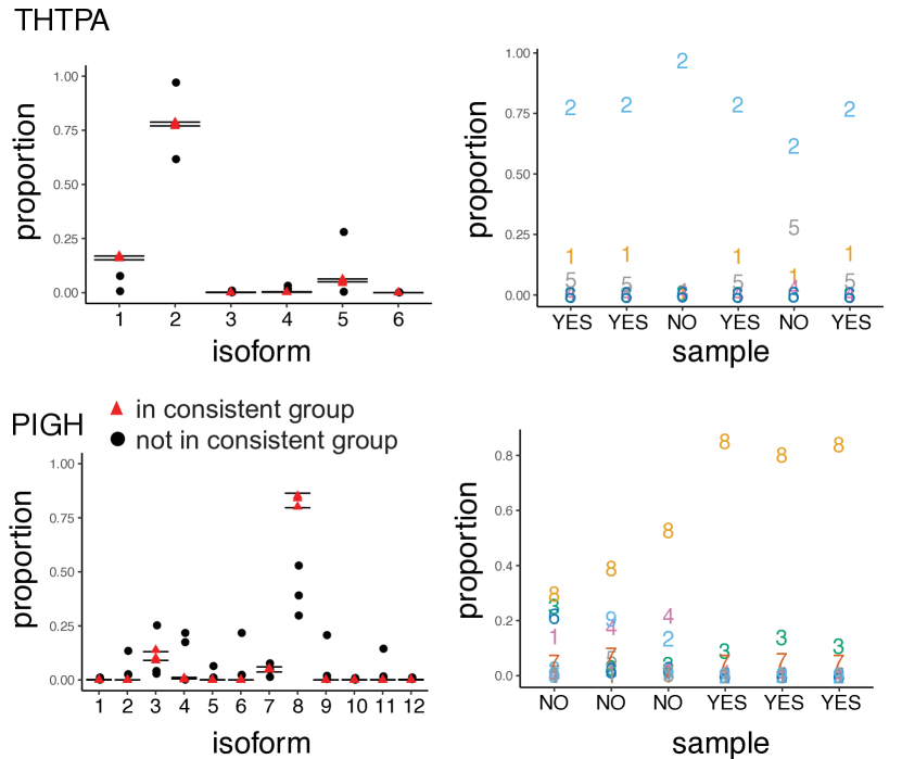
We also use set 1 (i.e., the $6$ hESC samples) in this study to illustrate why the consistent group represents more reliable transcriptome landscapes and how the standard deviation defined in formula (2.8) can be used to assess the biological variation within the consistent group. Shown in Figure 9 are two example genes THTPA ($6$ isoforms) and PIGH ($12$ isoforms). We use these two examples to illustrate that (1) MSIQ is bale to identify consistent groups that have comparably more consistent isoform abundances, and (2) the biological variation within the consistent group is much smaller compared to the overall variation among all the samples, and this variation is well captured by the estimated standard errors.

Figure 9: MSIQ’s estimated isoform proportions and standard errors for gene THTPA ($6$ isoforms) and gene PIGH ($12$ isoforms). The left plots give the estimated isoform proportions by isoform. The intervals are the respective MSIQ estimator $\pm$ one standard error: $\hat{\alpha}_{j}^{\text{MSIQ}}\pm\hat{\sigma}_{j}$. The right plots give the estimated isoform proportions by sample. The numbers denote the isoform indices and the horizontal axis denotes whether the corresponding sample is identified as being within the consistent group or not.

3.2.2 MSIQ leads to the highest correlation with NanoString counts

We present a second real data example to evaluate different methods by comparing their reported isoform abundances (in FPKM values) with NanoString counts on the same data sets. The NanoString nCounter technology is considered to be a highly reproducible and robust method for detecting gene and isoform expression (Kulkarni, 2011). As a consequence, the NanoString measurements are widely used as a benchmark for isoform expression (Germain et al., 2016; Steijger et al., 2013). We compare our MSIQ method with three other estimation methods, Cufflinks, iReckon, and MISO, based on their performances on six samples of the human HepG2 (liver hepatocellular carcinoma) immortalized cell line (see Supplementary Table S3 for detailed description).

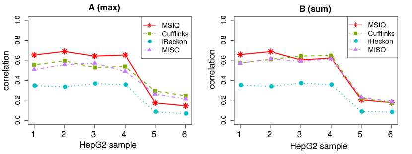
Even though genome-wide isoform abundances are not available for these HepG2 data, the NanoString counts are available for a small set of genes (Steijger et al., 2013). These NanoString measurements include $140$ probes that correspond to $470$ isoforms in $107$ genes. We apply MSIQ, Cufflinks, iReckon and MISO on the six HepG2 samples and use each method to estimate isoform abundances for this set of genes. Cufflinks and iReckon directly report the FPKM values of the relevant isoforms. MSIQ and MISO estimate isoform proportions, and the FPKM values can be calculated accordingly. For each sample, we calculate the Pearson correlation coefficient between each method’s estimated isoform expression and the benchmark NanoString counts. Since the NanoString probe counts do not have a one-to-one correspondence with isoform expression, for each NanoString probe we either use the isoform with the largest expression (Fig 10A) or add up the expression of all the isoforms (Fig 10B). Overall, the estimated expression of MSIQ has the highest correlation with the NanoString counts and achieves the best consistency with this benchmark measurement, compared with Cufflinks, iReckon and MISO. Please note that samples 5 and 6 are found not belonging to the consistent group by MSIQ, and that is why MSIQ does not have the highest correlations on them. This observation is coherent with the definition of a consistent group by MSIQ. This result again suggests that MSIQ leads to more accurate isoform quantification by incorporating the information in multiple RNA-seq samples.

Figure 10: Correlation between NanoString counts and the estimated isoform expression. A: For each NanoString probe, the corresponding isoform with the largest estimated FPKM value is used to calculate the correlation. The standard error of the calculated correlation coefficients is between $0.069$ and $0.099$. B: For each NanoString probe, the sum of all the corresponding isoforms’ estimated FPKM values is used to calculate the correlation. The standard error of the calculated correlation coefficients is between $0.065$ and $0.085$.

4 Discussion and conclusion

In this paper, we propose a new method, MSIQ, to more accurately estimate isoform expression levels associated with biological conditions of interest using multiple RNA-seq data sets. Accurate isoform quantification from RNA-seq data has long been a challenge because the existence of multiple isoforms makes it impossible to uniquely assign many reads and determine the reads’ isoform origins. MSIQ tackles this challenge by utilizing data from multiple RNA-seq samples derived from the same biological condition; we reason that aggregating more information can improve accuracy in isoform abundance estimation. Unlike previous work that treats all the samples equally, MSIQ identifies a consistent group of samples that are most representative of the biological condition and estimates isoform proportions of the consistent group.

Applications of MSIQ to both simulated and real data demonstrate that MSIQ yields more accurate isoform quantification than direct averaging or pooling methods given the existence of poor quality or mislabeled samples. These results suggest MSIQ’s potential as a powerful and robust transcriptomic tool for isoform expression quantification. MSIQ’s estimation results provide robust and accurate transcriptome profiles, which can be used to construct co-expression networks, investigate cell-type-specific isoform expression, and identify differentially expressed transcripts between two biological conditions. The MSIQ method also provides standard error estimates to measure the variability of isoform abundance within the consistent group. This information can be especially useful when users need to compare multiple tissue or cell types. We estimate the standard errors using the posterior samples of isoform proportions, and we note that our method can be extended to directly model the variability parameters at the cost of increased complexity in the model and computations. In addition to isoform abundance estimation, MSIQ can also be applied to evaluate the quality of multiple RNA-seq samples of the same tissue or cell type. This application can help researchers evaluate the reproducibility of RNA-seq samples and determine which samples to include in downstream analyses.

An important step in our MSIQ method is the identification of the consistent group, which depends on posterior draws of the hidden state variables. We currently use a Beta-Bernoulli model to describe the probability of each sample belonging to the consistent group. However, it is possible to improve the model once gold standard data (i.e., qPCR) for the biological condition of interest become available (Adamski et al., 2014; Li and Dewey, 2011). We can extend our MSIQ model to account for the heterogeneous quality of multiple RNA-seq samples based on the similarity of the isoform abundance estimates between each sample and the gold standard. Such quality assessment can be integrated with the inter-sample similarity to better identify the consistent group. As a result, the samples that have higher agreement with gold standards and high similarity with each other will be more likely to be considered a part of the consistent group. This procedure is supposed to identify more reliable samples and can potentially increase the re-use of public RNA-seq data as it will provide an interpretable measure of the quality of multiple RNA-seq data sets. We would also like to point out that biological knowledge can be incorporated into MSIQ modeling to further improve isoform abundance estimation. For example, mRNA fragments are, in fact, not uniformly distributed within the isoforms (Zhang et al., 2014), and a high correlation was observed between read coverage and genome GC content (Li et al., 2011). Our proposed hierarchical model can be considered an umbrella framework that can be easily extended to incorporate more detailed modeling procedures as long as these procedures use likelihoods to describe read generating processes. Such extension might help MSIQ achieve better performance on complex genes.

Another interesting extension of our MSIQ method is to model single-cell RNA-seq (scRNA-seq) data, which contain information on the technical and biological noise of isoform abundance at the single-cell level (Wu et al., 2014; Macaulay and Voet, 2014). scRNA-seq data are needed for the analysis of (1) subpopulations of cells from a larger heterogeneous population and (2) rare cell types, for which sufficient material cannot be obtained for conventional RNA-seq experiments (Mortazavi et al., 2008). Given scRNA-seq data on multiple cells from the same population, MSIQ can be iteratively utilized to evaluate the transcriptional heterogeneity and detect subpopulations (i.e., consistent groups) in the set of samples. Meanwhile, MSIQ can also reveal the principal isoform expression pattern in a given cell population. An alternative approach is to allow for multiple consistent groups as subpopulations of single cells in statistical modeling.

The RNA-seq data sets used in the paper are all publicly available. Their accession numbers are provided in the supplementary information. The MSIQ method is implemented in the R package MSIQ, which is freely available at https://github.com/Vivianstats/MSIQ.

Appendix A Figure Appendix

Figure A1: Relative estimation error (REE) rates of the seven estimators in scenario 1-5. REE rate are calculated on 3,421 fly genes with 3-98 exons. In each boxplot, the REE rates of MSIQ, AVG*, MSIQa, AVG, POOL*, MSIQp, and POOL are plotted side by side under each scenario (with the order of methods listed under the scenario 5 of the bottom left panel) and the whiskers extend to the most extreme REE rates. The top-right legend of each plot displays the parameter setting: the mean fragment length (F) and the read length (R).

See pages - of supplementary.pdf

References

- Adamski et al. (2014) Adamski, M. G., P. Gumann, and A. E. Baird (2014). A method for quantitative analysis of standard and high-throughput qpcr expression data based on input sample quantity. PloS one 9(8), e103917.
- Barrett et al. (2013) Barrett, T., S. E. Wilhite, P. Ledoux, C. Evangelista, I. F. Kim, M. Tomashevsky, K. A. Marshall, K. H. Phillippy, P. M. Sherman, M. Holko, et al. (2013). Ncbi geo: archive for functional genomics data sets—update. Nucleic acids research 41(D1), D991–D995.
- Behr et al. (2013) Behr, J., A. Kahles, Y. Zhong, V. T. Sreedharan, P. Drewe, and G. Rätsch (2013). Mitie: Simultaneous rna-seq-based transcript identification and quantification in multiple samples. Bioinformatics 29(20), 2529–2538.
- Bernard et al. (2014) Bernard, E., L. Jacob, J. Mairal, and J.-P. Vert (2014). Efficient rna isoform identification and quantification from rna-seq data with network flows. Bioinformatics, btu317.
- Collado-Torres et al. (2017) Collado-Torres, L., A. Nellore, K. Kammers, S. E. Ellis, M. A. Taub, K. D. Hansen, A. E. Jaffe, B. Langmead, and J. T. Leek (2017). Reproducible rna-seq analysis using recount2. Nature Biotechnology 35(4), 319–321.
- Conesa et al. (2016) Conesa, A., P. Madrigal, S. Tarazona, D. Gomez-Cabrero, A. Cervera, A. McPherson, M. W. Szcześniak, D. J. Gaffney, L. L. Elo, X. Zhang, et al. (2016). A survey of best practices for rna-seq data analysis. Genome biology 17(1), 1.
- Germain et al. (2016) Germain, P.-L., A. Vitriolo, A. Adamo, P. Laise, V. Das, and G. Testa (2016). Rnaonthebench: computational and empirical resources for benchmarking rnaseq quantification and differential expression methods. Nucleic acids research, gkw448.
- Griebel et al. (2012) Griebel, T., B. Zacher, P. Ribeca, E. Raineri, V. Lacroix, R. Guigó, and M. Sammeth (2012). Modelling and simulating generic rna-seq experiments with the flux simulator. Nucleic acids research 40(20), 10073–10083.
- Hansen et al. (2011) Hansen, K. D., Z. Wu, R. A. Irizarry, and J. T. Leek (2011). Sequencing technology does not eliminate biological variability. Nature biotechnology 29(7), 572–573.
- Harrow et al. (2012) Harrow, J., A. Frankish, J. M. Gonzalez, E. Tapanari, M. Diekhans, F. Kokocinski, B. L. Aken, D. Barrell, A. Zadissa, S. Searle, et al. (2012). Gencode: the reference human genome annotation for the encode project. Genome research 22(9), 1760–1774.
- Jiang and Wong (2009) Jiang, H. and W. H. Wong (2009). Statistical inferences for isoform expression in rna-seq. Bioinformatics 25(8), 1026–1032.
- Kanitz et al. (2015) Kanitz, A., F. Gypas, A. J. Gruber, A. R. Gruber, G. Martin, and M. Zavolan (2015). Comparative assessment of methods for the computational inference of transcript isoform abundance from rna-seq data. Genome biology 16(1), 1–26.
- Katz et al. (2010) Katz, Y., E. T. Wang, E. M. Airoldi, and C. B. Burge (2010). Analysis and design of rna sequencing experiments for identifying isoform regulation. Nature methods 7(12), 1009–1015.
- Kent et al. (2002) Kent, W. J., C. W. Sugnet, T. S. Furey, K. M. Roskin, T. H. Pringle, A. M. Zahler, and D. Haussler (2002). The human genome browser at ucsc. Genome research 12(6), 996–1006.
- Kulkarni (2011) Kulkarni, M. M. (2011). Digital multiplexed gene expression analysis using the nanostring ncounter system. Current Protocols in Molecular Biology, 25B–10.
- Li and Dewey (2011) Li, B. and C. N. Dewey (2011). Rsem: accurate transcript quantification from rna-seq data with or without a reference genome. BMC bioinformatics 12(1), 323.
- Li et al. (2011) Li, J. J., C.-R. Jiang, J. B. Brown, H. Huang, and P. J. Bickel (2011). Sparse linear modeling of next-generation mrna sequencing (rna-seq) data for isoform discovery and abundance estimation. Proceedings of the National Academy of Sciences 108(50), 19867–19872.
- Lin et al. (2012) Lin, Y.-Y., P. Dao, F. Hach, M. Bakhshi, F. Mo, A. Lapuk, C. Collins, and S. C. Sahinalp (2012). Cliiq: Accurate comparative detection and quantification of expressed isoforms in a population. In Algorithms in Bioinformatics, pp. 178–189. Springer.
- Macaulay and Voet (2014) Macaulay, I. C. and T. Voet (2014). Single cell genomics: advances and future perspectives. PLoS Genet 10(1), e1004126.
- Mezlini et al. (2013) Mezlini, A. M., E. J. Smith, M. Fiume, O. Buske, G. L. Savich, S. Shah, S. Aparicio, D. Y. Chiang, A. Goldenberg, and M. Brudno (2013). ireckon: Simultaneous isoform discovery and abundance estimation from rna-seq data. Genome research 23(3), 519–529.
- Mortazavi et al. (2008) Mortazavi, A., B. A. Williams, K. McCue, L. Schaeffer, and B. Wold (2008). Mapping and quantifying mammalian transcriptomes by rna-seq. Nature methods 5(7), 621–628.
- Pachter (2011) Pachter, L. (2011). Models for transcript quantification from rna-seq. arXiv preprint arXiv:1104.3889.
- Patro et al. (2014) Patro, R., S. M. Mount, and C. Kingsford (2014). Sailfish enables alignment-free isoform quantification from rna-seq reads using lightweight algorithms. Nature biotechnology 32(5), 462–464.
- Pruitt et al. (2014) Pruitt, K. D., G. R. Brown, S. M. Hiatt, F. Thibaud-Nissen, A. Astashyn, O. Ermolaeva, C. M. Farrell, J. Hart, M. J. Landrum, K. M. McGarvey, et al. (2014). Refseq: an update on mammalian reference sequences. Nucleic acids research 42(D1), D756–D763.
- Quail et al. (2012) Quail, M. A., M. Smith, P. Coupland, T. D. Otto, S. R. Harris, T. R. Connor, A. Bertoni, H. P. Swerdlow, and Y. Gu (2012). A tale of three next generation sequencing platforms: comparison of ion torrent, pacific biosciences and illumina miseq sequencers. BMC genomics 13(1), 1.
- Roberts and Pachter (2013) Roberts, A. and L. Pachter (2013). Streaming fragment assignment for real-time analysis of sequencing experiments. Nature methods 10(1), 71–73.
- Rosenbloom et al. (2015) Rosenbloom, K. R., J. Armstrong, G. P. Barber, J. Casper, H. Clawson, M. Diekhans, T. R. Dreszer, P. A. Fujita, L. Guruvadoo, M. Haeussler, et al. (2015). The ucsc genome browser database: 2015 update. Nucleic acids research 43(D1), D670–D681.
- Rossell et al. (2014) Rossell, D., C. S.-O. Attolini, M. Kroiss, and A. Stöcker (2014). Quantifying alternative splicing from paired-end rna-sequencing data. The annals of applied statistics 8(1), 309.
- Sakharkar et al. (2004) Sakharkar, M. K., V. T. Chow, and P. Kangueane (2004). Distributions of exons and introns in the human genome. In silico biology 4(4), 387–393.
- Steijger et al. (2013) Steijger, T., J. F. Abril, P. G. Engström, F. Kokocinski, T. J. Hubbard, R. Guigó, J. Harrow, P. Bertone, R. Consortium, et al. (2013). Assessment of transcript reconstruction methods for rna-seq. Nature methods 10(12), 1177–1184.
- Trapnell et al. (2009) Trapnell, C., L. Pachter, and S. L. Salzberg (2009). Tophat: discovering splice junctions with rna-seq. Bioinformatics 25(9), 1105–1111.
- Trapnell et al. (2010) Trapnell, C., B. A. Williams, G. Pertea, A. Mortazavi, G. Kwan, M. J. Van Baren, S. L. Salzberg, B. J. Wold, and L. Pachter (2010). Transcript assembly and quantification by rna-seq reveals unannotated transcripts and isoform switching during cell differentiation. Nature biotechnology 28(5), 511–515.
- Wang et al. (2009) Wang, Z., M. Gerstein, and M. Snyder (2009). Rna-seq: a revolutionary tool for transcriptomics. Nature Reviews Genetics 10(1), 57–63.
- Wu et al. (2014) Wu, A. R., N. F. Neff, T. Kalisky, P. Dalerba, B. Treutlein, M. E. Rothenberg, F. M. Mburu, G. L. Mantalas, S. Sim, M. F. Clarke, et al. (2014). Quantitative assessment of single-cell rna-sequencing methods. Nature methods 11(1), 41–46.
- Ye and Li (2016) Ye, Y. and J. J. Li (2016). Nmfp: a non-negative matrix factorization based preselection method to increase accuracy of identifying mrna isoforms from rna-seq data. BMC Genomics 17(1), 127.
- Zhang et al. (2014) Zhang, J., C.-C. J. Kuo, and L. Chen (2014). Wemiq: an accurate and robust isoform quantification method for rna-seq data. Bioinformatics, btu757.