The ExoMol database: molecular line lists for exoplanet and other hot atmospheres

Abstract

The ExoMol database (www.exomol.com) provides extensive line lists of molecular transitions which are valid over extended temperatures ranges. The status of the current release of the database is reviewed and a new data structure is specified. This structure augments the provision of energy levels (and hence transition frequencies) and Einstein $A$ coefficients with other key properties, including lifetimes of individual states, temperature-dependent cooling functions, Landé $g$-factors, partition functions, cross sections, $k$-coefficients and transition dipoles with phase relations. Particular attention is paid to the treatment of pressure broadening parameters. The new data structure includes a definition file which provides the necessary information for utilities accessing ExoMol through its application programming interface (API). Prospects for the inclusion of new species into the database are discussed.

tiny[table]font=tiny

1 Introduction

Hot molecules exist in many environments in space including cool stars [1], failed stars generally known as brown dwarfs [2, 1] and exoplanets [3]. The atmospheric properties of these objects are known to be strongly influenced by the spectra of the molecules they contain. On Earth, spectra of hot molecules are observed in flames [4, 5], discharge plasmas [6, 7], explosions [8] and in the hot gases emitted, for example, from smoke stacks [9]. In addition, high-lying states can be important in non local thermodynamic equilibrium (non-LTE) environments both in space, for example, emissions observed from comets [10, 11], and on Earth. The spectra of key atmospheric molecules at room temperature have been the subject of systematically maintained databases such as HITRAN [12, 13, 14] and GEISA [15, 16]. As will be amply illustrated below, the spectra of hot molecules contain many, many more transitions and so far attempts to compile systematic databases have been limited. Databases of hot molecular spectra do exist for other specialized applications, such as the EM2C database for combustion applications [17] or one due to Parigger et al for studies of laser-induced plasmas [18].

Planets and cool stars share some common fundamental characteristics: they are faint, their radiation peaks in the infrared and their atmosphere is dominated by strong molecular absorbers. Modelling planetary and stellar atmospheres is therefore difficult as their spectra are extremely rich in structure with hundreds of thousands to many billions of spectral lines which may be broadened by high-pressure and temperature effects.

The ExoMol project [19] aims to provide the molecular line lists that astronomers need in order to understand the physics and chemistry of astronomical bodies cool enough to form molecules in their atmospheres. In particular these data are needed for extrasolar planets, brown dwarfs and cool stars [20, 2, 3], as well as circumstellar structures such as planetary envelopes and molspheres [21]. In practice these data are also useful for a wide range of other scientific disciplines; examples include studies of the Earth’s atmosphere [22, 23], hypersonic non-equilibrium [24], analysis of laboratory spectra [25, 26, 27], measurements of hot reactive gases [28] and the proposed remote analysis of molecular composition using laser oblation [29].

The original ExoMol data structure was very focused in its goal, with the scope of the data limited to generating lists of transitions [30]. However, it has become obvious that the potential applications of the ExoMol spectroscopic data are much more diverse. For example, the ExoMol data can be used to compute partition functions [31], cross sections [32], lifetimes [33], Landé $g$-factors [34] and other properties. Our aim is to systematically provide this additional data to maximise its usefulness. To do this requires significant extension of the ExoMol data structure, which is the major purpose of this paper. At the same time this implementation should facilitate the adoption of an application programming interface (API) between the database and programs using it. Similar enhancements are actively being pursued by other related databases such as HITRAN [35, 36, 37]. A major new feature is the inclusion, albeit at a fairly crude level, of pressure-broadening parameters. These have been shown to be important for models of exoplanets [38, 39] and are known to be vital for many other applications. Section 2 summarizes current data coverage of the ExoMol database. Section 3 reviews the individual line lists included in the database with particular emphasis on any changes made to them since they were originally published. Section 4 describes the expansion of data that is now provided by the ExoMol database. Section 5 gives a formal description of the new data structures implemented to cover this provision and to provide the API functionality. Section 6 briefly describes the utility programs available as part of the ExoMol database and Section 7 the ExoMol website. Finally we discuss future prospects for the database.

2 Database coverage

The ExoMol project aims at complete coverage of the spectroscopic properties of molecules which are deemed to be important in hot astrophysical environments. Coverage concerns (a) the molecular species considered, including isotopologues; (b) the frequency range considered and (c) the upper temperature range for which the data is reasonably complete. Both the required temperature and frequency range completeness are to some extent a judgement on what is required for astronomical and other studies. For example, a molecule like nitric acid (HNO₃) will dissociate at a relatively low temperature so coverage above about 500 K is unlikely to be important. On the other hand, several diatomics such SiO and CO are known to feature in stellar spectra, and coverage to temperatures over 6000 K is necessary.

The general ExoMol approach is molecule-by-molecule. That is, a comprehensive line list is created for a particular molecule which is then made available in the database. For more challenging larger systems such as NH₃, PH₃ and HNO₃, it has been our policy to produce initial, room-temperature line lists, see [40, 41, 42] respectively. This allows us to improve the model, validate the available experimental data and, in some cases, make spectral assignments. In all instances, the subsequent hot line lists [43, 44, 45] are both more complete and more accurate and should therefore be used even for studies at low temperatures.

Thus far ExoMol has not considered ultraviolet (UV) absorption; however, there is increasing interest in the consequences of UV radiation on exoplanets [46, 47, 48] so this may need to be reviewed in future. As discussed in the comments below, molecules are still being added to the database so that coverage by species is steadily increasing.

Tables 1 and 2 summarize the molecules for which the ExoMol database currently provides data. The division is between species that have explicitly been studied as part of the ExoMol project (Table 1) and those for which the data has been taken from other studies (Table 2). The ExoMol project has a specific methodology based on the use of spectroscopically-determined potential energy surfaces and ab initio dipole surfaces, which are combined with explicit variational treatments of the nuclear motion problem. For open shell systems these treatments involve explicit inclusion of spin-orbit and related curve-coupling effects; the project has developed a nuclear motion program, Duo, for treating coupled diatomic curves [49]. For closed shell molecules a range of codes [50, 51, 52, 53, 54, 55] are used. These are all essentially based on finding near-exact solutions of the ro-vibrational Schrödinger equation for a given potential energy surface but the level of approximation increases with the size of the molecule considered.

Data from other sources arise from a variety of methodologies which range from completely ab initio, appropriate for systems with very few electrons, to largely empirical. Table 2 gives a pointer to the method used in each case; for full details the reader should consult the cited reference.

Table 1: Datasets created by the ExoMol project and included in the ExoMol database.

Molecule	$N_{\rm iso}$	$T_{\rm max}$	$N_{elec}$	$N_{\rm lines}$ a	DSName	Reference
BeH	1	2000	1	16 400	Yadin	Yadin et al [56]
MgH	3	2000	1	10 354	Yadin	Yadin et al [56]
CaH	1	2000	1	15 278	Yadin	Yadin et al [56]
SiO	5	9000	1	254 675	EJBT	Barton et al [57]
HCN/HNC	2a	4000	1	399 000 000	Harris	Barber et al [58]
CH4	1	1500	1	9 819 605 160	YT10to10	Yurchenko & Tennyson [59]
NaCl	2	3000	1	702 271	Barton	Barton et al [60]
KCl	4	3000	1	1 326 765	Barton	Barton et al [60]
PN	2	5000	1	142 512	YYLT	Yorke et al [61]
PH3	1	1500	1	16 803 703 395	SAlTY	Sousa-Silva et al [44]
H2CO	1	1500	1	10 000 000 000	AYTY	Al-Refaie et al [62]
AlO	4	8000	3	4 945 580	ATP	Patrascu et al [63]
NaH	2	7000	2	79 898	Rivlin	Rivlin et al [64]
HNO3	1	500	1	6 722 136 109	AlJS	Pavlyuchko et al [45]
CS	8	3000	1	548 312	JnK	Paulose et al [65]
CaO	1	5000	5	21 279 299	VBATHY	Yurchenko et al [66]
SO2	1	2000	1	1 300 000 000	ExoAmes	Underwood et al [67]

$N_{\rm iso}$ Number of isotopologues considered;
$T_{\rm max}$ Maximum temperature for which the line list is complete;
$N_{elec}$ Number of electronic states considered;
$N_{\rm lines}$ Number of lines: value is for the main isotope.
^a A line list for H¹³CN/HN¹³C due to Harris et al [68] is also available.

Table 2: Datasets not created as part of the ExoMol project but included in the ExoMol database.

Molecule	$N_{\rm iso}$	$T_{\rm max}$	$N_{elec}$	$N_{\rm lines}$	DSName	Reference	Methodology
H${}_{3}^{+}$	2a	4000	1	3 070 571	NMT	Neal et al [69]	ExoMol
H2O	2b	3000	1	505 806 202	BT2	Barber et al [70]	ExoMol
NH3	2c	1500	1	1 138 323 351	BYTe	Yurchenko et al [43]	ExoMol
HeH+	4	10000	1	1 431	Engel	Engel et al [71]	Ab initio
HD+	1	12000	1	10 119	CLT	Coppola et al [72]	Ab initio
LiH	1	12000	1	18 982	CLT	Coppola et al [72]	Ab initio
LiH+	1	12000	1	332	CLT	Coppola et al [72]	Ab initio
ScH	1	5000	6	1 152 827	LYT	Lodi et al [73]	Ab initio
MgH	1		3	30 896	13GhShBe	GharibNezhad et al [74]	Empirical
CaH	1		2	6000	11LiHaRa	Li et al [75]	Empirical
NH	1		1	10 414	14BrBeWe	Brooke et al [76]	Empirical
CH	2		4	54 086	14MaPlVa	Masseron et al [77]	Empirical
CN	1		1	195 120	14BrRaWe	Brooke et al [78]	Empirical
CP	1		1	28 735	14RaBrWe	Ram et al [79]	Empirical
HCl	1		1	2588	11LiGoBe	Ram et al [80]	Empirical
CrH	1		2	13 824	02BuRaBe	Burrows et al [81]	Empirical
FeH	1		2	93 040	10WEReSe	Wende et al [82]	Empirical
TiH	1		3	181 080	05BuDuBa	Burrows et al [83]	Empirical

$N_{\rm iso}$ Number of isotopologues considered;
$T_{\rm max}$ Maximum temperature for which the line list is complete;
$N_{elec}$ Number of electronic states considered;
$N_{\rm lines}$ Number of lines: value is for the main isotope.
^a There is a H₂D⁺ line list available from Sochi and Tennyson [84].
^b The VTT line list for HDO due to Voronin et al [85] is also available.
^c There is a room temperature ¹⁵NH₃ line list due to Yurchenko [86].

The molecules listed in Tables 1 and 2 do not at present provide a comprehensive set of species. A number of key species are available from other sources. HITEMP [87] in principle provides a source of data for CO, OH, NO and CO₂. In practice there are new hot line lists for CO [88], OH [89], and CO₂ [90, 91] which are more recent than the data given in the current release of HITEMP. High quality line lists for ozone are also available from elsewhere [92]. Line lists for some other missing species may also be found in the UGAMOP (https://www.physast.uga.edu/ugamop/) and Kurucz [93] databases. The coverage of these databases for a (possible) exoplanet characterization mission has recently been reviewed by two of us [94]. VALD3, the latest release of the Vienna atomic line database, contains line lists for a small number of diatomics [95].

Finally we note that while the majority of exoplanet spectroscopy is performed at rather low resolution, very precise spectroscopic data can be required [96, 97, 98], which is proving an issue for particular key species [99]. Therefore, ExoMol aims to be both complete, and as accurate as possible.

3 Individual line lists

Below we consider some of the line lists presented in the ExoMol database and listed in Tables 1 and 2. We restrict our discussion to issues not covered in the original publication.

One general issue is that Medvedev and co-workers [100, 88] identified a numerical problem with the intensities of high overtone transitions computed with the standard compilation of the diatomic vibration-rotation program Level [50]. Our line lists computed with Level have been adjusted to remove transitions which appeared to have been affected by this issue; such cases are noted below. The transitions removed are all very weak and it is anticipated that these changes will have very little effect on practical applications. We checked similar calculations performed with our in-house rovibronic program Duo [49] and found similar behaviour: when the value of the transition dipole moment becomes comparable with the double precision error ($\approx 10^{-16}$ a.u.), the corresponding electric dipole intensities essentially represent numerical noise and have to be removed.

3.1 MgH

The ExoMol MgH line list only considers transitions within the X ${}^{2}\Sigma^{+}$ ground electronic state [56]. A line list containing A ${}^{2}\Pi$ – X ${}^{2}\Sigma^{+}$ and B^′ ${}^{2}\Sigma^{+}$ – X ${}^{2}\Sigma^{+}$ transitions has been given by GharibNezhad et al [74]. Both line lists are included in the ExoMol database.

Furthermore Szidarovszky and Császár [101] showed that, due to the relatively low dissociation energy of MgH, consideration of quasi-bound states in the partition sum significantly alters the partition function at higher temperatures. However, for reasons of self-consistency we recommend using the partition function given by Yadin et al [56].

3.2 CaH

The ExoMol CaH line list only considers transitions within the X ${}^{2}\Sigma^{+}$ ground electronic state [56]. A line list containing E ${}^{2}\Pi$ – X ${}^{2}\Sigma^{+}$ transitions has been given by Li et al [75]. Both line lists are included in the ExoMol database.

3.3 SiO

The original SiO ExoMol line lists of Barton et al [57] computed using Level have been truncated by removing transitions with $\Delta v\geq 6$.

3.4 HCN/HNC

The combined HCN/HNC Exomol line list of Barber et al [58] used a calculated energy separation (isomerization energy) of 5705 cm^-1 between the ground states of HCN and HNC. Recent work by Nguyen et al [102] suggests that this value is too high. We have done some additional ab initio calculation using MOLPRO [103] at multi-reference configuration interaction (MRCI) level of theory. The complete basis set extrapolation (CBS) value CBS[56]z was found to equal 5356 cm^-1. Substracting from this value the zero point energy difference between HCN and HNC wells of 88 cm^-1, gives the value for the energy separation of 5268 cm^-1, consistant with the value of 5236 $\pm$ 50 cm^-1 recommended by Nguyen et al[102]. This value has been adopted by revising the states file and calculated partition function.

3.5 CH₄

Although the YT10to10 line list [59] represents a major step forward in the modelling of hot methane spectra [104], it does not represent a complete solution to the problem. Rey et al [105] have also produced a line list, using similar procedures to those adopted by ExoMol, valid to higher temperatures (2000 K) but covering a more limited spectral range. The temperature coverage can be checked using available, high-temperature partition functions [106, 107].

Yurchenko et al [108] have extended the YT10to10 line list to higher temperatures (2000 K) and improved the predicted frequencies by replacing computed energy levels with empirical ones provided by Boudon [109]. The resulting line list has 35 billion transitions and Yurchenko et al propose that most of the lines in the line list can be represented by background cross sections. These temperature-dependent, but pressure-independent cross sections, generated using the vast majority of the lines, can then be used to supplement a reduced line list of 203 million lines selected to be the strongest in each spectral region. If this methodology proves successful, it will be adopted by the ExoMol database for other very extensive line lists in future releases. At present these data are not included in the database.

3.6 NaCl

The original NaCl ExoMol line lists of Barton et al [60] computed using Level have been truncated by removing transitions with $\Delta v\geq 8$.

3.7 KCl

The original KCl ExoMol line lists of Barton et al [60] computed using Level have been truncated by removing transitions with $\Delta v\geq 12$.

3.8 PN

The original PN ExoMol line lists of Yorke et al [61] computed using Level have been truncated by removing transitions with $\Delta v\geq 6$.

3.9 AlO

A number of ExoMol users pointed out that the vibrational labels used in the original AlO line list were not the best ones. Our analysis of AlO state lifetimes [110] reinforced this impression. The .states file has therefore been updated with revised vibrational state labels. We note that these labels are only approximate quantum numbers and this change should not affect any results obtained with the line list.

3.10 H${}_{3}^{+}$

The H${}_{3}^{+}$ line list of Neal et al [69] (NMT) is the oldest in the ExoMol database. While it has continued to demonstrate its accuracy and predictive power [111, 112], perhaps surprisingly so, there are other issues with it. The line list was constructed using Jacobi coordinates which do not allow for a full treatment of the symmetry. This led to the use of approximate nuclear spin statistical weights and, more problematically, to the removal of very weak transitions. Most of these transitions are symmetry-forbidden and should have zero dipole intensity. However “forbidden” rotational transitions [113, 114] have proved important for both astrophysical [115, 116] and laboratory [117, 118] studies. Methods are available which allow for the proper treatment of symmetry [119, 120]. A new line list [121] is nearly complete which extends the range of the NMT line list. The upper energy limit is increased to 25 000 cm^-1 and the highest rotational quantum number state considered in the calculations is $J=40$. This line list will remove the symmetry problem as well as improve both the accuracy and coverage for H${}_{3}^{+}$, thus making it useful for both higher and lower temperatures.

3.11 H₂O

The BT2 line list [70] has been outstandingly successful: it was used for the original detection of water in an exoplanet atmosphere [122], forms the basis of the well-used BT-Settl brown-dwarf model [123] and provides the hot water line list for HITEMP [87]. However, although it is more complete, for many levels it is less accurate than the Ames line list of Partridge and Schwenke [124]. Since the construction of BT2 there has been significant progress in deriving experimental energy levels for H₂¹⁶O [125, 126], improvements in the ab initio dipole moment surface [127] which have been used to construct high accuracy room temperature line lists [128] and further improvements in representing the potential energy surface of the molecule [129]. A new H₂¹⁶O line list, named POKAZATEL, [130] which builds on these advances will be released soon. The completeness of this line list is illustrated by the following figures: The highest rotational quantum number used in the calculations of the wavefunctions was $J=72$ — close to the highest $J$ for wich the bound states still do exist. The highest upper energy levels limit is equal to 40 000 cm^-1, which is also close to the dissociation limit of water [131].

While the BT2 and Ames line lists are seriously incomplete for temperatures above 3000 K, POKAZATEL considers every ro-vibrational transition in the molecule and therefore is appropriate for studies at higher temperatures.

Line lists for hot H₂¹⁷O and H₂¹⁸O will also be released very shortly [132]. Again these will take advantage of the available set of experimental energy levels [133, 134] obtained using the MARVEL procedure [135, 136]. These line lists will be as complete as BT2 and consider levels with $J\leq 50$ and energies up to 30 000 cm^-1.

3.12 NH₃

Ammonia is a ten electron system like water, so in terms of electronic calculations one might expect similar improvements here too. ¹⁴NH₃ has also been the subject of a systematic study of experimental energy levels [137] and improvements in its ab initio treatment [138, 139]. New experimental data characterizing higher-lying energy levels is also available [26, 140]. Again the Ames group have performed high accuracy studies on this system [138, 141, 142], although there is no corresponding line list. Work is therefore in progress to compute a new ammonia line list which will replace the existing BYTe line list [43]; in particular this work the option of using the improved nuclear motion capability of the program TROVE working in curvilinear coordinates [54]. Recent, excellent ab initio calculations [139] which reproduce very highly excited energy levels of ammonia up to 18 000 cm^-1, will be used as the starting point for a semi-empirical fit of the PES. This should give a line list which is both more accurate and more extensive than BYTe.

3.13 CrH

Chromium hydride is an important astronomical molecule for a variety of reasons, including classification of brown dwarfs [143, 144] and measurements of magnetic fields [145]. The ExoMol database currently provides a substantially empirical line list due to Burrows et al [81]; we are in the process of computing a more complete CrH line list covering 8 states and the 4 main isotopologues [146].

3.14 TiH

The current titanium hydride line list due to Burrows et al [83] is in the process of being updated with a more extensive ExoMol one.

3.15 Other species

Besides the species listed above, line lists are in an advanced stage of construction for VO [147], H₂O₂ [148] (see Al-Refaie et al [149] for a preliminary, room temperature version), SO₃ [150] (see also Underwood et al [151]), C₂H₄, CH₃Cl (see also Owens et al [152]), C₂ (see also Furtenbacher et al [153]), SiH, NS, NO, NaO, AlH and SH [154], MnH, and PO, PS and PH [155].

Finally we note that work is in progress looking at TiO [156]. TiO is a major absorber in cool stars [157, 158]. There are TiO line lists available from Schwenke [159], Plez [160] and VALD3 [95]. However it would appear that these line lists are incomplete; in particular there are missing bands that have been observed in the laboratory [161]. Furthermore, recent exoplanet studies suggest that the line frequencies are too inaccurate for high resolution studies [99].

4 Data Provided

The original aim of the ExoMol project was the provision of extensive line lists of energy levels, and hence transition frequencies, and Einstein $A$ coefficients from which transition intensities and related information can be computed. The original ExoMol data structure [30] provided precisely for these data in a concise manner. The demands on and utility of the data provided by the project has led us to expand the scope of the database. In this section we outline the new data provision and in the following sections we formally define the new data structures employed for this purpose.

4.1 Extended states file

There are other properties of a molecular state that can be computed by ExoMol which we now propose to store. The first of these is the radiative lifetime of each individual state, which can be computed in a straightforward fashion from the Einstein $A$ coefficients [33]. Such lifetimes have been shown to be important in both laboratory [117, 118] and astronomical [115, 116] environments. Indeed the radiative lifetime of a state is a key component in determining the critical density of species in that state and hence whether it exists in local thermodynamic equilibrium (LTE) in a given environment. Our recent study of lifetimes based on use of ExoMol data suggested that methane should show particularly interesting lifetime effects [33]. These computed lifetimes can be compared with experimental measurements, where available, providing a check on our calculated dipole moments. This is particularly useful for rovibronic spectra, where measurements of absolute transition intensities are unusual.

The second state-dependent property are Landé $g$-factors. These provide the behaviour of the states in the presence of a weak magnetic field as given by the Zeeman effect. Molecular spectra can provide important information on magnetic fields in stars, brown dwarfs and exoplanets [145, 162]. For open shell diatomics, Landé $g$-factors are given by a fairly straightforward formula in terms of standard Hund’s case (a) quantum numbers [163]. The vibronic wavefunctions computed by Duo [49] contain the necessary information to compute these $g$-factors and this has currently recently been implemented within Duo [34]. The magnetic fields in some astronomical environments are strong enough that the Paschen-Back effect becomes important [145, 164]. In this case the shifts in the energy levels do not have a simple dependence on the magnetic field [165] and they will have to be explicitly computed on a case-by-case basis. Landé $g$-factors are only given for systems whose spectroscopic model includes open shell electronic states (ie ones with unpaired electrons) since these are the systems whose states which show significant splitting in a magnetic field.

Besides (approximate) quantum numbers, which may appear in several forms, it is also often desirable to store more than one estimate of the energy level of the state. A general methodology, known as MARVEL, is available for obtaining self-consistent sets of empirical energy levels from networks of transitions [135, 136], which means that sets of empirical energy levels are available for key molecules [133, 134, 125, 166, 167, 153]. In this case it is preferable to replace computed energy levels with empirical ones, as has already been done for the HCN/HNC [58] and the CS [65] line lists. It is also recommended to keep the original computed levels as well as the uncertainties which are generally available for the empirical levels. The inclusion of approximate quantum numbers and extra energy levels included has been decided on a molecule-by-molecule basis; information on this is contained in the isotopologue definition file (see Section 5.3).

4.2 Cross sections, $k$-coefficients and pressure effects

Many of the line lists stored in the database are huge. This makes finding other forms of storing the data desirable. ExoMol data has been used to generate temperature-dependent cross sections as a function of wavenumber [32]. Such cross sections now form part of the database which will also be expanded to contain pressure-dependent cross sections and $k$-coefficient tables generated from them.

Cross sections depend on pressure, as well as temperature, due to collisional broadening by the species in the atmosphere. The provision of temperature-, pressure- and broadening species-dependent cross sections would be both computationally very demanding and again result in very large datasets. Instead we have chosen to primarily provide parameters which characterise pressure profiles for key species plus software allowing cross sections to be generated for selected temperature-pressure parameters on the user’s own computer. There is a widespread recognition that for detailed studies, such as those performed in the Earth’s atmosphere at high resolution, Voigt profiles only provide an approximate solution to the problem [168]. However Voigt profiles are in widespread use and are easily computed [169]; they are therefore used to represent pressure broadening effects in ExoMol.

The new release of ExoMol includes, where possible, pressure broadening parameters. So far, these have not been considered for vibronic spectra. HITRAN provides a source of air-broadening and self-broadening parameters [170] so in the absence of other sources these are taken from HITRAN 2012 [171]. In gas giants H₂ and He are the major broadeners. There is no systematic source of parameters for these broadeners so we have to treat each system on a case-by-case basis. While some work has been performed for broadening of hot water by H₂ and He [172, 16], more data would clearly be helpful in this area. Hedges and Madhusudhan [39] recently put this in context by quantifying the effects of various factors involved in modelling line broadening in exoplanetary atmospheres, including completeness of broadening parameters, on molecular absorption cross sections.

ExoMol will provide Lorentzian half-widths and their temperature-exponents for key molecule-broadener systems. The availability of these parameters varies with species and broadener. In any case there are not individual values for every molecular line and often parameters have only been measured or calculated for a small fraction of transitions. Therefore, rather than pre-determine values for every molecular line and increase the size of the line lists, which are very large for some molecules, a separate pressure broadening parameters file is provided. This file contains three types of parameters: experimental, theoretical and semi-empirical. Experimental, theoretical and semi-empirical parameters from the literature are presented with their respective full or partial quantum number assignments. Additional semi-empirical parameters are determined by compiling all experimental and theoretical parameters as a function of $J^{\prime\prime}$, the total rotational quantum number of the lower level of the transition, and computing an average value for each $J^{\prime\prime}$. To avoid introducing additional error, no extrapolation is attempted beyond the $J^{\prime\prime}_{\rm max}$ for which data are available, the parameters are simply assumed to be constant from this point. This is a very basic model similar to that used by other line-width studies [173, 174, 175]. Constructing the pressure broadening parameters file in this way ensures that parameters are provided for every spectral line. Table LABEL:tab:broad_ref lists the main sources used to provide pressure broadening parameters. Clearly further and improved parameters would be welcome.

Table 3: Sources of pressure broadening parameters for key molecule-broadener species currently being considered by ExoMol. Entries marked ^∗ were extracted from HITRAN [171, 176].

Molecule	Broadener	Reference	Methodology
H2O	H2	Lavrentieva et al [177]	Semi-empirical
		Lavrentieva et al [178]	Semi-empirical
		Steyert et al [179]	Experimental
		Brown & Plymate [180]	Experimental
		Brown et al [181]	Experimental
		Gamache et al [182]	Theoretical
		Dick et al [183]	Experimental
		Faure et al [172]	Theoretical
		Langlois et al [184]	Experimental
		Dutta et al [185]	Experimental
		Golubiatnikov [186]	Semi-empirical
		Zeninari et al [187]	Semi-empirical
		Drouin and Wiesenfeld [188]	Theoretical
H2O	He	Lavrentieva et al [177]	Semi-empirical
		Lavrentieva et al [178]	Semi-empirical
		Steyert et al [179]	Experimental
		Gamache et al [182]	Theoretical
		Dick et al [183]	Experimental
		Lazarev et al [189]	Experimental
		Dutta et al [185]	Experimental
		Golubiatnikov [186]	Semi-empirical
		Zeninari et al [187]	Semi-empirical
H2O	Air	Mérienne et al [190]∗	Experimental
		Gamache & Hartmann [191]∗	Semi-empirical
		Gasster et al [192]∗	Experimental
		Payne et al [193]∗	Experimental
		Gamache [194]∗	Semi-empirical
		Gamache & Laraia [195]	Semi-empirical
H2O	H2O	Mérienne et al  [190]∗	Experimental
		Gamache & Hartmann [191]∗	Semi-empirical
		Markov [196]∗	Experimental
		Golubiatnikov et al [197]∗	Experimental
		Cazzoli et al [198]∗	Semi-empirical
CH4	H2	Pine [199]	Experimental
		Margolis [200]	Experimental
		Fox et al [201]	Experimental
		Strong et al [202]	Experimental
CH4	He	Pine [199]	Experimental
		Varanasi & Chudamani[203]	Experimental
		Gabard et al [204]	Experimental
		Grigoriev et al [205]	Semi-empirical
		Fox et al [201]	Experimental
CH4	Air	Predoi-Cross et al [206]∗	Experimental
		Smith et al [207]∗	Experimental
		Brown et al [208]∗	Semi-empirical
		Anthony et al [209]	Theoretical
CH4	CH4	Predoi-Cross et al [210]∗	Experimental
		Smith et al [211]∗	Experimental
		Brown et al [208]∗	Semi-empirical
NH3	H2	Pine et al [212]∗	Experimental
		Hadded et al [213]∗	Experimental
		Sharp & Burrows [214]∗	Semi-empirical
NH3	He	Pine et al [212]∗	Experimental
		Hadded et al [213]∗	Experimental
		Sharp & Burrows [214]∗	Semi-empirical
NH3	Air	Brown & Peterson [215]∗	Experimental
NH3	NH3	Brown & Peterson [215]∗	Experimental
PH3	H2	Bouanich et al [216]	Semi-empirical
		Levy et al [217]	Experimental
		Sergent-Rozey et al [218]	Experimental
		Salem et al [219]	Experimental
		Pickett et al [220]	Experimental
		Levy et al [221]	Experimental
PH3	He	Salem et al [222]	Experimental
		Levy et al [217]	Experimental
		Sergent-Rozey et al [218]	Experimental
		Pickett et al [220]	Experimental
		Levy et al  [221]	Experimental
PH3	Air	Butler et al [223]∗	Experimental
		Kleiner et al [224]∗	Semi-empirical
PH3	PH3	Butler et al [223]∗	Experimental
		Kleiner et al [224]∗	Semi-empirical
H2CO	H2	Nerf [225]	Experimental
H2CO	He	Nerf [225]	Experimental
H2CO	N2	Jacquemart et al [226]	Semi-empirical
H2CO	H2O	Jacquemart et al [226]∗	Semi-empirical
HCN	Air	Yang et al [227]∗	Experimental
		Devi et al [228]∗	Semi-empirical
		Risland et al [229]∗	Semi-empirical
HCN	HCN	Devi et al [228]∗	Semi-empirical
		Devi et al [230]∗	Semi-empirical
CS	Air	Blanquet et al [231]∗	Semi-empirical
CS	CS	Misago et al [232]∗	Semi-empirical

Another compact form of data input to exoplanet modelling codes involves the use of the $k$-coefficient approximation [233, 234, 235], for example, by the NEMESIS code [236] and cross sections, as used by Tau-REx [237, 238, 239]. Temperature- and pressure-dependent $k$-coefficients are also been provided for certain key species.

4.3 Partition and cooling functions

In practice the ExoMol project always required partition functions, the study of which has often been performed independently [240, 241, 242, 31], and on occasion adopted from other studies [106]. Temperature-dependent partition functions are now formally included as part of the data structure.

Of course in various environments such as the early Universe and regions of star or planetary formation, the transformation of energy into radiation through molecular emissions provide an important source of cooling. Temperature-dependent cooling functions are important [243, 72, 244] and can also be computed from ExoMol line lists [33]. These are also now included in the data structure.

4.4 Dipoles

While Einstein $A$ coefficients are sufficient for the vast majority of radiative transport applications, the construction of these loses the phase information contained in the individual, complex-valued transition dipole moments. Incorporating the phase information in the ExoMol database will make it useful for theoretical modelling of the effects of an electric field on molecular structure. The areas of application includes cooling and trapping of molecular beams (see Ref. [245] and references therein), manipulating the long-range molecular interactions and collisional dynamics [246, 247, 248], molecular orientation and alignment [249, 250, 245], as well as rotational spectroscopy [251, 252, 253, 254]. As shown in Section 5.7, the absolute values of transition dipole moments can be computed from the Einstein $A$ coefficients and it is sufficient to complement this with only the sign of transition dipole moment for each molecular line.

4.5 Spectroscopic Models

In addition to the spectroscopic data provided by the ExoMol database, each ExoMol line list has been constructed from a detailed spectroscopic model of the given molecule. In general this model includes a (spectroscopically-determined) potential energy surface and ab initio dipole moment surfaces, and input to the appropriate nuclear motion program. For systems with multiple electronic states, the spectroscopic model also includes coupling between electronic states, e.g. spin-orbit, electronic angular momentum etc.

These spectroscopic models are a valuable product of the ExoMol procedure and there are several reasons for preserving them. Firstly, the spectroscopic model is ultimately the source of error in the final line list and is thus important when investigating discrepancies between experiment or astronomical observations and theoretical predictions. Secondly, they can be used as a starting point for future models or line lists. For example, new experimental data can be incorporated through refinement of potential energy curves; improved ab initio methodologies can be incorporated by improvements to the dipole moment surface, or further electronic states can be added to the model. Finally, they can be useful for other applications besides calculation of the original line list. Current work within the ExoMol group is investigating the sensitivity of spectral lines to a possible variation in the proton-to-electron mass ratio [255, 256].

An important part of each spectroscopic model is the input file to the appropriate nuclear motion program (e.g. Level [50], Duo [49], DVR3D [51], TROVE [53]). For the diatomic codes Level and Duo, the program input generally includes full details of the appropriate (potential, dipole and coupling) curves [257]. For the polyatomic nuclear motion programs DVR3D and TROVE, the PES and DMS are provided as standalone functions, usually written in Fortran, with the program inputs as separate files. These spectroscopic models are not part of the formal ExoMol data structure described in the next section but can be accessed from the webpage of the appropriate isotopologue in files labelled .model.

5 Data Structures

The data structure outlined below represents a significant extension of the original ExoMol data structure described by Tennyson et al [30]. However the core structure of the two files, the states and transitions files, used in the original specification remains unchanged meaning that utilities designed to work with the previous structure will still work.

A summary of the contents of the database is stored in a master file, exomol.all. This file points towards the files which store the actual data. Table 4 gives an overview of these files, which are available for each isotopologue under the updated ExoMol structure. Each of these files is specified in turn below. Figure 1 gives a schematic representation of the file structure of the ExoMol data.

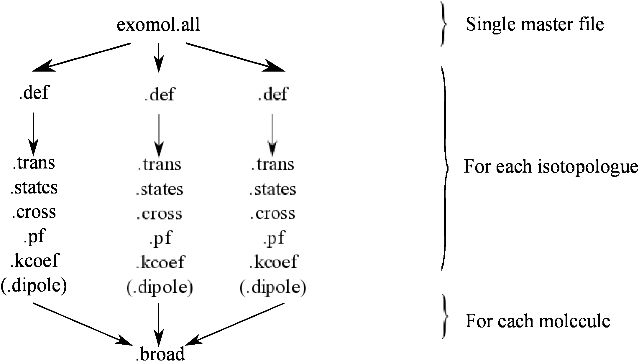
Figure 1: Structure of the ExoMol data files. There is a single master file describing the database, $N_{\rm mol}$ molecules and $N_{\rm iso}$ files per molecule.

Table 4: Specification of the ExoMol file types. (Contents in brackets are optional.)

File extension	$N_{\rm files}$	File DSname	Contents
.all	1	Master	Single file defining contents of the ExoMol database..
.def	$N_{\rm tot}$	Definition	Defines contents of other files for each isotopologue.
.states	$N_{\rm tot}$	States	Energy levels, quantum numbers, (lifetimes), (Landé $g$-factors).
.trans	a	Transitions	Einstein $A$ coefficients, (wavenumber).
.broad	$N_{\rm mol}$	Broadening	Parameters for pressure-dependent line profiles.
.cross	b	cross sections	Temperature or temperature and pressure-dependent cross sections.
.kcoef	c	$k$-coefficients	Temperature and pressure-dependent $k$-coefficients.
.pf	$N_{\rm tot}$	Partition function	Temperature-dependent partition function, (cooling function).
.dipoles	$N_{\rm tot}$	Dipoles	Transition dipoles including phases.
.overview	$N_{\rm mol}$	Overview	Overview of datasets available.
.readme	$N_{\rm iso}$	Readme	Specifies data formats.
.model	$N_{\rm iso}$	Model	Model specification.

$N_{\rm files}$ total number of possible files.
$N_{\rm mol}$ Number of molecules in the database
$N_{\rm tot}$ is the sum of $N_{\rm iso}$ for the $N_{\rm mol}$ molecules in the database
$N_{\rm iso}$ Number of isotopologues considered for the given molecule
^a There are $N_{\rm tot}$ sets of .trans files but for molecules with large numbers of transitions the .trans files are subdivided into wavenumber regions.
^b There are $N_{\rm cross}$ sets of .cross files for isotopoplogue.
^c There are $N_{\rm kcoef}$ sets of .kcoef files for each isotopoplogue.

5.1 File naming convention

The naming convention for the files in the ExoMol database has the following specification. All file names, with the exception of the Pressure Broadening file, have a common part built using the template Iso-slug__LineList__. The “Iso-slug” is a machine-readable, plain ASCII-text “XML-safe” unique identifier for the molecular isotopologue, for example, 14N-1H3 is the iso-slug for ¹⁴NH₃. Ions are denoted by an appended ’_mZ’ or ’_pZ’ for charges $-Z$ and $+Z$ respectively (with the value of Z omitted if it is unity); so 1H3_p is the iso-slug for ¹H${}_{3}^{+}$. “Linelist” is the line list publication name, see the column “DSName” in Tables 1 and 2; for example, the published names for the ¹⁴NH₃ and H${}_{3}^{+}$ line lists are BYTe and NMT respectively. For external datasets that have been cast in ExoMol format, this name is an 8 character year-authors string which follows the convention of the IUPAC Task Group on water spectroscopy [133]. The extensive bibliography files, in BibTeX format, provided on the ExoMol website for each molecule in the database, uses the same naming convention.

This common part of the file name can be followed by additional identifiers specific to different file types. For example, the transition file .trans for polyatomic molecules is usually split into smaller wavenumber ranges in order to simplify the manipulation of data. In this case the Iso-slug__LineList__ is followed by NUMIN-NUMAX, which specifies the wavenumber range in cm^-1. The absorption cross section .cross file names also contain a wavenumber range, representing the full coverage of the line list, followed by the temperature in Kelvin, pressure in bar and the binning interval, or resolution (in cm^-1), for which the cross sections have been computed. The file names have the form NUMIN-NUMAX__Temperature[K]__Pressure[bar]__resolution after the common part.

In the case of the Pressure Broadening file .broad, the file name does not contain the string LineList__ as the data in the broadening files is not line list specific and has been compiled from a number of sources. Here the string Iso-slug__ is simply followed by Broadener identifying the broadener.

For example, the current BT2 line list package consists of the definition file 1H2-16O__BT2.def, the States file 1H2-16O__BT2.states, sixty Transitions files: 1H2-16O__BT2__00000-00500.trans, 1H2-16O__BT2__00500-01000.trans, …1H2-16O__BT2__29500-30000.trans, Partition function file 1H2-16O__BT2.pf, Pressure Broadening files: 1H2-16O__H2.broad, 1H2-16O__He.broad, 1H2-16O__air.broad, 1H2-16O__self.broad and eighteen cross section files: 1H2-16O__BT2__00000-30000__296K__0bar__0.01.cross, 1H2-16O__BT2__00000-30000__400K__0bar__0.01.cross, …1H2-16O__BT2__00000-30000__900K__0bar__0.01.cross, 1H2-16O__BT2__00000-30000__1000K__0bar__0.01.cross, 1H2-16O__BT2__00000-30000__1200K__0bar__0.01.cross, …1H2-16O__BT2__00000-30000__3000K__0bar__0.01.cross,

Here 1H2-16O is the iso-slug for H${}_{2}{}^{16}$O, BT2 is the name of the water line list [70], 00000-00500 is the wavenumber range 0–500 cm^-1, H₂, He, air and self are the broadeners, 296 K is the temperature, 0 bar is the pressure and 0.01 is the binning interval for the cross sections in wavenumbers.

For most cases a single .broad file is provided for a given molecule and designated for the parent (most abundant) isotopologue. Should broadening parameters be required for other isotopologues, this file should be employed. In a few cases where isotopic substitution lowers the symmetry, e.g. HDO as compared to H₂O, then extra isotopologue-specific broadening files may be provided, although thus far there are no such files.

Table 5: Format of the ExoMol master file, exomol.all; each entry starts on a new line.

Field	Fortran Format	C Format	Description
Header Information
ID	A13	%13s	Always the ASCII string “EXOMOL.master”
$V_{\rm all}$	I8	%8d	Version number, format YYYYMMDD, recording
			last update of the whole database
$N_{\rm mol}$	I4	%4d	Number of molecules in the database
Followed by $N_{\rm mol}$ entries of the form
Molecule Information
$N_{\rm name}$	I3	%3d	Number of molecule names listed.
Followed by $N_{\rm name}$ entries of the form
MolName	A27	%27s	(Common) name of the molecule
MolFormula	A27	%27s	Molecule chemical formula
$N_{\rm iso}$	I4	%4d	Number of isotopologues considered
MolKey	A27	%27s	Inchi key of the isotopologue
IsoFormula	A27	%27s	Isotopologue chemical formula
Iso-slug	A160	%160s	Isotopologue slug identifier, see text for details
DSName	A10	%10s	Isotopologue dataset name
$V$	I8	%8d	Version number with format YYYYMMDD
Metadata			Free format

5.2 The master file

The file exomol.all is designed to be machine searchable making it easy to check the current contents of the database and when any of it was last updated. The file is structured as a list of molecules with the isotopologues associated with that molecule. The actual ExoMol data files are stored by isotopologue. Table 5 specifies the format of the file while Table LABEL:tab:alleg gives a portion of the current contents for water with two isotopologues, H₂¹⁶O and HD¹⁶O. The final entry gives web-searchable meta-data.

Table 6: Extract from the exomol.all master file showing the three line header and the portion for the water molecule.

EXOMOL.master	# ID
20160315	# Version number with format YYYYMMDD
30	# Number of molecules in the database
1	# Number of molecule names listed
water	# Name of the molecule
H2O	# Molecule chemical formula
2	# Number of isotopologues considered
XLYOFNOQVPJJNP-DYCDLGHISA-N	# Inchi key of molecule
(1H)(2H)(16O)	# Iso-slug
1H-2H-16O	# IsoFormula
VTT	# Isotopologue dataset name
20160314	# Version number with format YYYYMMDD
XLYOFNOQVPJJNP-UHFFFAOYSA-N	# Inchi key of molecule
(1H)2(16O)	# Iso-slug
1H2-16O	# IsoFormula
BT2	# Isotopologue dataset name
20160220	# Version number with format YYYYMMDD

5.3 The definition file

A new addition to the ExoMol format is the inclusion of the definition file with extension .def. The definition file gives information on what ExoMol provides for a particular isotopologue and describes how the data can be used. The definition file serves multiple purposes:

• Standardized ExoMol file usage: The ExoMol format [30] .states file contains 4 standard fields: The ID of the state, the energy, the total degeneracy and the $J$ quantum number. However additional fields such as the symmetry and vibrational quantum numbers are not standardized and differ between molecules. For usage that requires these additional quantum numbers, a subroutine or function must be created for each molecule to be read. The definition file therefore provides a means to overcome this by providing a single subroutine with the information to read any states file provided by the ExoMol project. This allows codes to easily integrate the ExoMol format only once and provide support for all molecules in the ExoMol project without additional changes.

• Improved database function: The definition file also provides detailed information on all fields in the ExoMol format. This means that database functionality such as sorting, filtering, splitting, selecting etc on specific or multiple fields can be easily performed on single or multiple molecules.

• Facilitated updates: Finally, updates of particular molecules can be easily propagated to any user of the ExoMol format. Each definition file is assigned a version number; this allows the user to check whether there are any updates to a particular molecule, with the possibility of an automatic download of any modified files and immediate usage without change to codes.

The format is defined in Table LABEL:tab:def_format. The data format can be subdivided into different sections (highlighted in bold) describing a different aspect of the molecule in the ExoMol format. Each section may contain multiple subsections that define further aspects of that section. The file format therefore takes a tree structure. An example definition file for the CS line list [65] is given in Table. LABEL:tab:CS_example and for the BT2 water line list [70] in Table. LABEL:tab:BT2_example.

5.3.1 Header

The first section describes metadata related to internal molecular data. $V$ is the version number of the definition file, it utilises a numerical dating format $YYYYMMDD$ in order to allow for easy chronological ordering of different versions by integer comparison. The MolKey is the 27 character InchiKey [258] used to identify the molecule and $N_{\rm atom}$ describes the number of atoms in the molecule. This allows code to modify its behaviour based on whether it is dealing with diatomic molecules $N_{\rm atom}=2$ or polyatomics $N_{\rm atom}>2$.

Table 7: Definition file format; each entry starts on a new line.

Field	Fortran Format	C Format	Description
Header Information
ID	A10	%10s	Always the ASCII string “EXOMOL.def”
IsoFormula	A27	%27s	Isotopologue chemical formula
Iso-slug	A160	%160s	Isotopologue identifier, see text for details
DSName	A10	%10s	Isotopologue dataset name
$V$	I8	%8d	Version number with format YYYYMMDD
MolKey	A27	%27s	Standard inchi key of the molecule
$N_{\rm atom}$	I4	%4d	Number of atoms
Atom definition (The following 2 lines occur $N_{\rm atom}$ times)
$I_{\rm atom}$	I3	%3d	Isotope number
Atom	A3	%3s	Element symbol
Isotopologue Information
$m_{Da}\quad m_{kg}$	F12.6,1X,ES14.8	%12.6f %14.8e	Isotopologue mass in Da and kg
$I_{\rm sym}$	A6	%6s	Molecular symmetry Group (if $N_{\rm atom}=2$ then C or D)
$N_{\rm irrep}$	I4	%4d	Number of irreducible representations
Symmetry definitions (The following 3 lines occur $N_{\rm irrep}$ times)
$I_{\rm irrep}$	I3	%3d	Irreducible representation ID
Symmetry	A6	%6s	Irreducible representation label
$g_{\rm ns}$	I3	%3d	Nuclear spin degeneracy
ExoMol Information
$T_{\rm max}$	F8.2	%8.2f	Maximum temperature of the line list
$N_{\rm broad}$	I3	%3d	No. of pressure broadeners available
$D_{\rm avail}$	I2	%2d	Dipole availability (1=Yes 0=No)
$N_{\rm cross}$	I3	%3d	No. of cross section files available
$N_{\rm kcoef}$	I3	%3d	No. of $k$-coefficient files available
States file information
Lifeavail	I2	%2d	Flag denoting lifetime availability (1=Yes 0=No)
$g_{\rm avail}$	I2	%2d	Flag denoting Landé $g$-factor availability (1=Yes 0=No)
$N_{\rm states}$	I10	%10d	No. of states in .states file
$N_{\rm cases}$	I3	%3d	No. of quanta cases
Quanta case definition (The following line occurs $N_{\rm cases}$ times)
Case Label	A8	%8s	Label of the quanta case
$N_{\rm quanta}$	I3	%3d	No. of quanta defined
Quanta definition (The following 3 lines occur $N_{\rm quanta}$ times)
Quanta Label	A3	%3s
$F_{\rm Fortran}\quad F_{\rm C}$	A8,1X,A8	%8s %8s	Fortran and C format for quanta
Description	A40	%40s	Short description of quanta
Trans file definition
$N_{\rm trans}$	I15	%15d	Total number of transitions
$N_{\rm files}$	I4	%4d	Number of transition files
$\tilde{v}_{\rm max}$	F8.2	%8.2f	Maximum wavenumber (in cm-1)
$E_{\rm lower}$	F8.2	%8.2f	Higher energy with complete set of transitions (in $cm^{-1}$)
Partition function information
$T^{Q}_{\rm max}$	F8.2	%8.2f	Maximum temperature of partition functions
$T_{\rm Step}$	F5.2	%5.2f	Temperature step size
$C_{\rm avail}$	I2	%2d	Cooling function availability (1=Yes 0=No)
Pressure Broadening Information (default values)
$\gamma_{D}$	F6.4	%6.4f	Default value of Lorentzian half-width for all lines (in cm-1/bar)
$n_{D}$	F5.3	%5.3f	Default value of the temperature exponent for all lines
Pressure Broadening Information ($N_{\rm broad}>0$, the following 6 lines occur $N_{\rm broad}$ times)
Broadener Label	A8	%8s	Label for particular broadener
Broadener File Name A20		%20s	File name of particular broadener
$J_{\rm max}$	I7/F7.1	%7d/%7.1f	Maximum $J^{\prime\prime}$ for which pressure broadened parameters are provided
$\gamma_{L}$	F6.4	%6.4f	Value of Lorentzian half-width for lines with $J^{\prime\prime}>J_{\rm max}$ (in cm-1/bar)
$n_{L}$	F5.3	%5.3f	Value of the temperature exponent for lines with $J^{\prime\prime}>J_{\rm max}$
$N_{Q}$	I4	%4d	Number of defined quantum number sets
Quantum Sets (The following 3 lines occur $N_{Q}$ times)
Set Code	A2	%2s	A code that defines this set of quantum numbers
$N_{\rm lines}$	I6	%6d	No. of lines in the broad that contain this code
$N_{\rm Quanta}$	I4	%4d	No. of quantum numbers defined
Quantum Numbers (The following line occurs $N_{\rm Quanta}$ times)
Quantum Label	A4	%4s

5.3.2 Atom Definition

This section describes each of the atoms in the molecule. The $N_{\rm atom}$ field describes how many of them are defined. An integer mass number and a string of the molecule allows a definite description of the isotopologue.

5.3.3 Isotopologue Information

This section gives mass and symmetry information about the molecules. $m$ is the molecular mass given in both Da and kg; the mass is used for modeling Doppler broadening. Next is the symmetry information of the molecule. The molecular symmetry group [259] and number of irreducible representations (irreps), $N_{\rm irrep}$, are described here, after which $N_{\rm irrep}$ lines defining each irrep in that group are given. The $I_{\rm sym}$ field gives the ID of the symmetry used in the .states file. However, for linear molecules including diatomics the symmetry group label will only take values of C or D corresponding to $C_{\infty v}$ or $D_{\infty h}$ respectively and $N_{\rm sym}$ is set to 0. $g_{\rm ns}$ corresponding to nuclear spin degenracy will be provided for C. For D, $g_{\rm even}$ and $g_{\rm odd}$ are provided; these correspond to the nuclear-spin degeneracy factor needed for when the rovibronic wavefunction (i.e. the wavefunction without nuclear spin) is respectively even or odd with respect to interchange of identical atoms. Otherwise we follow symmetry labels and conventions as set out by Bunker and Jensen [259]. In this case $g_{\rm ns}$ is be provided for each irreducible representation.

5.3.4 ExoMol Information

This section relates to the availability of certain aspects of the line list. First and foremost it describes the maximum temperature for which the line list is applicable ($T_{\rm max}$). Secondly, for molecules with pressure broadening parameters, it describes the number of broadeners ($N_{\rm broad}$) available; this is used later on to determine what additional structures should be parsed in the file. Finally, there is a boolean field which describes whether we provide dipoles for the particular molecule.

5.3.5 State file information

This section is the most important as it describes how the .states file format is structured. The first two fields describe whether lifetime information and Landé $g$-factors are available. These will be placed after the initial ‘standard’ fields in the states file. Then there is the $N_{\rm states}$ field which gives the number of states in the file. Finally the number of quanta cases, $N_{\rm cases}$. A quanta case describes what the following quantum numbers represent. For example, commonly for polyatomics the ExoMol .states file provides two representations of quantum numbers; the standard normal mode quantum numbers and the local mode ‘TROVE’ quantum numbers. For this example $N_{\rm cases}=2$; see Down et al [14] for instance; a recent review of local modes has been given by Jensen [260]. Each case is given a label and must describe the number of quanta defined $N_{\rm quanta}$, after which $N_{\rm quanta}$ lines will follow, each describing a particular quantum number. Quantum numbers are described by a string label comprising a string format identifier and a short, human-readable description. The string format identifier utilises the FORTRAN string formatting to allow for the construction of formats more easily for FORTRAN which has stricter string handling than C/C++. An overview of the new .states format is given in Section 5.4.

5.3.6 Transition and partition information

This section simply describes the availability of .trans and .pf files. In particular, for the partition function file (.pf) it describes the maximum temperature provided ($T^{Q}_{\rm max}$), the step size of the temperature ($T_{\rm Step}$) and whether a cooling function is also present.

5.3.7 Pressure broadening information

Finally, the pressure broadening information is provided here. If $N_{\rm broad}=0$ this simply contains default values of Lorentzian half-width $\gamma_{L}$ and temperature exponent $n_{L}$. If $N_{\rm broad}>0$ this section has the following structure: the broadener is defined first, immediately followed by the associated file name, $J_{\rm max}$, and the asymptotic values of the Lorentzian half-width $\gamma_{D}$ and temperature exponent $n_{D}$ for the $a0$ quantum number set (see Section 5.6). $N_{Q}$ quantum number sets are explicitly defined by a label (e.g. $a0$) that corresponds to codes in the broadener file, the number of lines in the broadener file with that code and the number of quantum numbers in that set. After this each additional quantum number is also described; the total angular momentum quantum number of the lower state $J"$ is compulsory. The quantum numbers relate to the quanta defined previously in the states section followed by either a prime or double prime. Further details relating to pressure broadening are given in Section 5.6.

The final field of the definition file is used for keywords to facilitate the search of the database by web search engines.

Table 8: File 12C-32S__JnK.def: the definition file for ¹²C³²S.

EXOMOL.def	# ID
(12C)(32S)	# IsoFormula
12C-32S	# Iso-slug
JnK	# Isotopologue data set name
20160217	# Version number with format YYYYMMDD
DXHPZXWIPWDXHJ-UHFFFAOYSA-N	# Inchi key of molecule
2	# Number of atoms
12	# Isotope number 1
C	# Element symbol 1
32	# Isotope number 2
S	# Element symbol 2
43.972071 7.30173406e-26	# Isotopologue mass (Da) and (kg)
C	# Symmetry group
2	# Number irreducible representations
1	# Irreducible representation ID
Sigma+	# Irreducible representation label
1	# Nuclear spin degeneracy
2	# Irreducible representation ID
Sigma-	# Irreducible representation label
1	# Nuclear spin degeneracy
3000	# Maximum temperature of linelist
2	# No. of pressure broadeners available
0	# Dipole availability (1=yes, 0=no)
0	# No. of cross section files available
0	# No. of k-coefficient files available
0	# Lifetime availability (1=yes, 0=no)
0	# Lande g-factor availability (1=yes, 0=no)
11497	# No. of states in .states file
1	# No. of quanta cases
dcs	# Quantum case label
1	# No. of quanta defined
v	# Quantum label 1
I4 %4d	# Format quantum label 1
State vibrational quantum number	# Description quantum label 1
199045	# Total number of transitions
1	# No. of transition files
10996.09	# Maximum wavenumber (in cm-1)
30000.00	# Higher energy with complete set of transitions (in cm-1)
3000.0	# Maximum temperature of partition function
1.00	# Temperature step size
0	# Cooling function availability (1=yes, 0=no)
0.0700	# Default value of Lorentzian half-width for all lines (in cm-1/bar)
0.500	# Default value of temperature exponent for all lines
air	# Label for a particular broadener
12C-32S__air.broad	# Filename of particular broadener
46	# Maximum J for which pressure broadening parameters provided
0.0698	# Value of Lorentzian half-width for J" > Jmax
0.750	# Value of temperature exponent for lines with J" > Jmax
1	# Number of defined quantum number sets
a0	# A code that defines this set of quantum numbers
47	# No. of lines in the broad that contain this code
0	# No. of quantum numbers defined
self	# Label for a particular broadener
12C-32S__self.broad	# Filename of particular broadener
46	# Maximum J for which pressure broadening parameters provided
0.0620	# Value of Lorentzian half-width for J" > Jmax
0.500	# Value of temperature exponent for lines with J" > Jmax
1	# Number of defined quantum number sets
a0	# A code that defines this set of quantum numbers
47	# No. of lines in the broad that contain this code
0	# No. of quantum numbers defined

Table 9: File BT2.def: the definition file for H₂¹⁶O.

EXOMOL.def	# ID
(1H)2(16O)	# IsoFormula
1H2-16O	# Iso-slug
BT2	# Isotopologue
20160220	# Version number with format YYYYMMDD
XLYOFNOQVPJJNP-UHFFFAOYSA-N	# Inchi key of molecule
3	# Number of atoms
1	# Isotope number 1
H	# Element symbol 1
16	# Isotope number 2
O	# Element symbol 2
18.010565 2.99072463e-26	# Isotopologue mass (Da) and (kg)
C2v	# Symmetry group
4	# Number of irreducible representations
1	# Irreducible representation ID
A1	# Irreducible representation label
1	# Nuclear spin degeneracy
2	# Irreducible representation ID
A2	# Irreducible representation label
1	# Nuclear spin degeneracy
3	# Irreducible representation ID
B1	# Irreducible representation label
3	# Nuclear spin degeneracy
4	# Irreducible representation ID
B2	# Irreducible representation label
3	# Nuclear spin degeneracy
3000.0	# Maximum temperature of linelist
0	# No. of pressure broadeners available
0	# Dipole availability (1=yes, 0=no)
0	# No. of cross section files available
0	# No. of k-coefficient files available
0	# Lifetime availability (1=yes, 0=no)
0	# Lande g-factor availability (1=yes, 0=no)
221097	# No. of states in .states file
1	# No. of quanta cases
nltcs	# Quantum case label
10	# No. of quanta defined
+/-	# Quantum label 1
A1 %1s	# Format quantum label 1
Total parity	# Description quantum label 1
Gamma	# Quantum label 3
I2 %2d	# Format Quantum label 2
Symmetry block number (1)	# Description Quantum label 2
N	# Quantum label 3
I10 %10d	# Format Quantum label 3
Reference within the symmetry block	# Description Quantum label 4
nucspin	# Quantum label 4
A1 %1s	# Format Quantum label 4
Nuclear spin isomer label(2)	# Description Quantum label 5
Gamma_rve	# Quantum label 5
A2 %2s	# Format Quantum label 5
Rovibrational symmetry label	# Description Quantum label 6
v1	# Quantum label 6
I2 %2d	# Format Quantum label 6
v1 symmetric stretch quantum number(3	# Description Quantum label 7
v2	# Quantum label 7
I2 %2d	# Format Quantum label 7
v2 bend quantum number	# Description Quantum label 8
v3	# Quantum label 8
I2 %2d	# Format Quantum label 8
v2 asymmetric stretch quantum number	# Description Quantum label 9
Ka	# Quantum label 9
I2 %2d	# Format Quantum label 9
Ka rotational quantum number	# Description Quantum label 10
Kc	# Quantum label 10
I2 %2d	# Format Quantum label 10
Kc rotational quantum number	# Description quantum label 10
505806255	# Total number of transitions
16	# No. of transition files
29971.78	# Maximum wavenumber (in cm-1)
20000.00	# Higher energy with complete set of transitions (in cm-1)
3000.0	# Maximum temperature of partition function
1.0	# Step size of temperature
1	# Cooling function availability (1=yes, 0=no)
0.0700	# Default value of Lorentzian half-width for all lines (in cm-1/bar)
0.500	# Default value of temperature exponent for all lines

5.4 States file

The basic ExoMol data structure is a comprehensive list of the molecular states involved. This file contains a numbered list of energy terms, in cm^-1 with the zero defined by the lowest level, immediately followed by the total statistical weight $g_{\mathrm{tot}}=(2J+1)\times g_{\rm ns}$ in the HITRAN convention [261] which retains the full nuclear-spin degeneracy of all atoms. These three columns are sufficient, in conjunction with the transitions file, to model absorption and/or emission intensities. The degeneracy is followed by the total angular momentum quantum number $J$ (integer or half-integer). The next columns are used for the state lifetimes (s) and/or Landé $g$-factors with availability determined in the definition file. This is followed by good (rigorous) quantum number(s) such as the state symmetry, parity or a total symmetry (irreducible representation). Then follows any approximate quantum numbers that are specified. There is some flexibility over this portion of the file which is defined on a case-by-case basis, see Ref. [262] for example.

For polyatomic molecules the approximate quantum numbers include, for example, the vibrational normal mode $v_{i}$, local mode $n_{i}$ quantum numbers, rotational quantum numbers $K$, $K_{a}$, $K_{c}$, polyad numbers, vibrational and rotational symmetries etc. For the diatomic molecules these are the spin components $F_{i}$, $\Sigma$ or $\Omega$, electronic term designations, e.g ${}^{3}{}\Pi_{g}$, vibrational quantum numbers $v$, rotational angular momentum $N$ (Hund’s case (b)), projection of the electronic angular momentum, $\Lambda$, etc. The spin components quantum numbers can be integral, half-integral or even strings F1, F2, $\ldots$ If the theoretical energy is replaced by an experimental counterpart, the former is usually kept as an extra field.

Regardless of molecule, the structure of any ExoMol state file can be determined from its complimentary definition file. The structure in order is:

1. Mandatory fields

2. Lifetime if Life${}_{\rm avail}=1$

3. Landé $g$-factor if $g_{\rm avail}=1$

4. Quanta Cases in order of definition

The detailed specification of the mandatory section of the states file is given in Table 10. Using the state file information from Table LABEL:tab:CS_example, the mandatory definition in the FORTRAN string format can easily be programmatically generated:

"(I12,1x,F12.6,1x,I6,1x,I7,1x,ES12.4,1x,A1,1x,A1,1x,A9,1x,I2,1x,I2,1x,I2,1x,I2)"

This format corresponds to the sample state file given in Table 11.

Note that for lifetimes it is necessary to deal with states with infinite radiative lifetimes (e.g. the ground state) and for which lifetimes are not available: for high-lying states not all downward transitions are considered so it is not possible to compute the lifetime. Here, and elsewhere in the database, infinity is specified by the string ‘INF’ and unknown numbers by ‘NaN’.

Table 10: Specification of the mandatory part of the states file and extra data options.

Field	Fortran Format	C Format	Description
$i$	I12	%12d	State ID
$E$	F12.6	%12.6f	State energy in $\mathrm{cm^{-1}}$
$g_{\mathrm{tot}}$	I6	%6d	State degeneracy
$J$	I7/F7.1	%7d/%7.1f	$J$-quantum number (integer/half-integer)
($\tau$)	ES12.4	%12.4e	Lifetime in s (optional)
($g$)	F10.6	%10.6f	Landé $g$-factor (optional)

ID: state identifier: a non-negative integer index, starting at 1

$J$: total angular momentum quantum, excluding nuclear spin

Fortran format, $J$ integer: (I12,1x,F12.6,1x,I6,I7,1x,ES12.4,1x,F10.6)
or $J$ half-integer: (I12,1x,F12.6,1x,I6,F7.1,1x,ES12.4,1x,F10.6)

Table 11: Extract from the state file for ⁴⁰Ca¹⁶O, 40Ca-16O__VBATHY.state.

$i$	$\tilde{E}$	$g$	$J$	$\tau$	$g$	$+/-$	$e/f$	State	$v$	$\Lambda$	$\Sigma$	$\Omega$
4051	8242.235601	15	7	6.5090E-01	0.106733	+	f	a3Pi	0	1	1	2
4052	8294.404892	15	7	2.1060E-03	0.018230	+	f	a3Pi	0	1	0	1
4053	8369.059680	15	7	4.5940E-01	0.000045	+	f	a3Pi	0	1	-1	0
4054	8627.261523	15	7	6.4790E-05	0.017893	+	f	Ap1Pi	0	1	0	1
4055	8781.692232	15	7	1.8810E-01	0.106728	+	f	a3Pi	1	1	1	2
4056	8833.629438	15	7	1.4660E-03	0.018239	+	f	a3Pi	1	1	0	1
4057	8907.535275	15	7	1.5950E-01	0.000048	+	f	a3Pi	1	1	-1	0
4058	9167.417952	15	7	4.4060E-05	0.017996	+	f	Ap1Pi	1	1	0	1
4059	9314.686162	15	7	1.0190E-01	0.106678	+	f	a3Pi	2	1	1	2
4060	9365.515048	15	7	1.1390E-03	0.018390	+	f	a3Pi	2	1	0	1
4061	9434.128287	15	7	7.8210E-02	0.000113	+	f	a3Pi	2	1	-1	0
4062	9533.168336	15	7	2.1600E-03	0.029567	+	f	b3Sigma+	0	0	1	1
4063	9545.896549	15	7	1.1140E-02	0.005414	+	f	b3Sigma+	0	0	0	0
4064	9709.239641	15	7	3.3420E-05	0.018256	+	f	Ap1Pi	2	1	0	1
4065	9841.636252	15	7	8.9050E-02	0.106743	+	f	a3Pi	3	1	1	2
4066	9893.716709	15	7	1.0390E-03	0.018284	+	f	a3Pi	3	1	0	1
4067	9966.036778	15	7	6.8230E-02	0.000061	+	f	a3Pi	3	1	-1	0
4068	10103.239512	15	7	1.1060E-03	0.026224	+	f	b3Sigma+	1	0	1	1
4069	10115.858820	15	7	2.8870E-03	0.008900	+	f	b3Sigma+	1	0	0	0
4070	10240.534926	15	7	2.7290E-05	0.018317	+	f	Ap1Pi	3	1	0	1

$i$: State counting number.

$\tilde{E}$: State energy in cm^-1.

$g$: State degeneracy.

$J$: Total angular momentum.

$\tau$: Lifetime in s.

$g$: Landé $g$-factor

$+/-$: Total parity.

$e/f$: rotationless-parity.

$v$: State vibrational quantum number.

$\Lambda$: Projection of the electronic angular momentum.

$\Sigma$: Projection of the electronic spin.

$\Omega$: $\Omega=\Lambda+\Sigma$, projection of the total angular momentum.

5.5 Transitions file

The transitions file has a simple structure, see Table 12. Two pointers, $i$ and $f$ point to rows in the .states file to identify the upper and lower states involved plus the full information characterising these states. The $A$ gives the Einstein $A$ coefficient for this transition. This file can be very large but, optionally, there is a fourth column $\tilde{\nu}$ which gives the transition wavenumber. Otherwise this must be computed from the states file as the difference of the upper and lower energy levels. A sample transitions file is given in Table 13.

Many of the molecules in the database are characterised by a very large number of transitions. To make the use of .trans tractable these files are often split into wavenumber regions, as discussed above. The .trans files are also compressed using .bz2 format; a utility is provided for reading this format without needing to uncompress the file.

Table 12: Specification of the transitions file.

Field	Fortran Format	C Format	Description
$i$	I12	%12d	Upper state ID
$f$	I12	%12d	Lower state ID
$A$	ES10.4	%10.4e	Einstein $A$ coefficient in $\mathrm{s^{-1}}$
$\tilde{\nu}_{fi}$	F15.6	%15.6f	Transition wavenumber in cm-1 (optional).

Fortran format: (I12,1x,I12,1x,ES10.4,1x,ES15.6)

Table 13: Extract from the transitions file for ⁴⁰Ca¹⁶O, 40Ca-16O__VBATHY.trans.

$i$	$f$	$A_{if}$	$\tilde{\nu}_{if}$
10571	10884	9.5518E-06	120.241863
21053	21375	1.9515E-05	120.242886
8726	9672	1.8658E-04	120.243522
11655	11950	5.0065E-06	120.243733
93209	93967	5.7055E-03	120.244192
2228	3175	7.3226E-07	120.244564
46727	46432	1.0599E-04	120.244658
44436	44774	1.4626E-04	120.245583
29037	28723	1.8052E-04	120.245669
4458	4805	1.0431E-08	120.246396
69313	68434	5.0531E-06	120.248178
22640	22985	1.1281E-07	120.248891
57027	56721	7.1064E-06	120.250180

$i$: Upper state counting number;
$f$: Lower state counting number; $A_{if}$: Einstein $A$
coefficient in s^-1; $\tilde{\nu}_{if}$: transiton wavenumber in cm^-1.

5.6 Pressure broadening file

Table 14: Specification of the mandatory part of the pressure broadening parameters file.

Field	Fortran Format	C format	Description
code	A2	%2s	Code identifying quantum number set following $J^{\prime\prime}$
$\gamma_{\textrm{ref}}$	F6.4	%6.4f	Lorentzian half-width at reference temperature and pressure in cm-1/bar
$n$	F6.3	%6.3f	Temperature exponent
$J^{\prime\prime}$	I7/F7.1	%7d/%7.1f	Lower $J$-quantum number integer/half-integer

Fortran format, $J$ integer: (A2,1x,F6.4,1x,F6.3,1x,I7)
or $J$ half-integer: (A2,1x,F6.4,1x,F6.3,1x,F7.1)

Like the .states file, the first four fields of the .broad file are mandatory for all records, see Table 14. This includes one quantum number, $J^{\prime\prime}$, which is always known and hence guarantees that at least a semi-empirical Lorentzian half-width ($\gamma_{\textrm{ref}}$) and temperature dependence, represented by exponent $n$ (see Eq. 1), can be generated for every molecular line. Additional upper and lower state labels, which give molecule and quantum number dependent behavior, follow the compulsory fields. These are given in the definitions file along with the maximum $J^{\prime\prime}$ for which approximate parameters have been generated, $J^{\prime\prime}_{\rm max}$, and the respective values of Lorentzian half-width and temperature exponent, $\gamma_{\rm max}$ and $n_{\rm max}$. When $J^{\prime\prime}>J^{\prime\prime}_{\rm max}$, $\gamma_{\rm max}$ and $n_{\rm max}$ should be used for the Lorentzian half-width and temperature exponent respectively.

The .broad file has a hierarchical structure; values of $\gamma_{\textrm{ref}}$ and $n$ with full quantum assignments are presented first, followed by values with partial quantum assignments, then finally values with $J^{\prime\prime}$ dependence only. This represents the preferential order in which the values of $\gamma_{\textrm{ref}}$ and $n$ should be used. This hierarchical structure is demonstrated in Table 16 where a portion of the H₂O-H₂ .broad file is presented.

Once a suitable $\gamma_{\rm ref}$ and $n$ have been identified, the Lorentzian half-width of a spectral line at temperature $T$ and pressure $P$ can be calculated as:

$$\gamma(T)=\gamma_{\textrm{ref}}\times\left(\frac{T_{\textrm{ref}}}{T}\right)^{n}\times\left(\frac{P}{P_{\textrm{ref}}}\right).$$ (1)

Here, $T_{\textrm{ref}}$ = 296 K and $P_{\textrm{ref}}$ = 1 bar. Note that to convert from cm^-1/bar used by ExoMol to cm^-1/atm used by Hitran requires $\gamma$ to be mutiplied by 1.01325.

A separate .broad file is supplied for each molecule-broadener system and the broadener is specified in the file name. Example.broad files for CS-Air and H₂O-H₂ are given in Table 15 and Table 16. For particular molecule-broadener systems where no pressure broadening information is available, the default values of $\gamma_{\textrm{ref}}$ and $n$ given in the isotopologue’s definition file may be used.

Table 15: File 12C-32S__air.broad: Air .broad file for ¹²C³²S: portion of the file (upper part); field specification (lower part).

a0	0.0860	0.096	0
a0	0.0850	0.093	1
a0	0.0840	0.091	2
a0	0.0840	0.089	3
a0	0.0830	0.087	4
…
a0	0.0720	0.067	35
a0	0.0720	0.066	36
…

Field	Fortran Format	C format	Description
code	A2	$\%$2s	Code identifying quantum number set following $J^{\prime\prime}$*
$\gamma_{\textrm{ref}}$	F6.4	%6.4f	Lorentzian half-width at reference temperature and pressure in cm-1/bar
$n$	F5.3	%5.3f	Temperature exponent
$J^{\prime\prime}$	I7/F7.1	$\%$7d	Lower $J$-quantum number

*Code definition: a0 = none

Table 16: 1H2-16O__H2.broad: H₂O - H₂ broad file: portion of the file (upper part); field specification (lower part).

…
b2	0.0356	0.300	9	8	1	9	0	8	0	0	0	0	1	0
b2	0.0522	0.300	9	8	1	9	0	8	0	0	0	1	0	0
b2	0.0521	0.300	7	8	1	6	1	7	0	0	0	0	0	1
…
a5	0.0600	0.546	3	4	0	3	1	4
a5	0.0618	0.551	3	4	2	1	1	4
a5	0.0569	0.525	2	3	2	1	3	0
…
a1	0.0301	0.268	14	15
a1	0.0291	0.230	15	16
a1	0.0282	0.218	16	17
…
a0	0.0242	0.165	24
a0	0.0239	0.160	25
a0	0.0236	0.150	26
…

Field	Fortran Format	C format	Description
code	A2	$\%$2s	Code identifying quantum number set following $J^{\prime\prime}$*
$\gamma_{\textrm{ref}}$	F2.4	%2.4f	Lorentzian half-width at reference temperature and pressure in cm-1/bar
$n$	F2.3	%2.3f	Temperature exponent
$J^{\prime\prime}$	I7	$\%$7d	Lower $J$-quantum number
$J^{\prime}$	I7	$\%$7d	Upper $J$-quantum number
$K_{a}^{\prime\prime}$	I2	$\%$2d	Lower rotational quantum number
$K_{c}^{\prime\prime}$	I2	$\%$2d	Lower rotational quantum number
$K_{a}^{\prime}$	I2	$\%$2d	Upper rotational quantum number
$K_{c}^{\prime}$	I2	$\%$2d	Upper rotational quantum number
$v_{1}^{\prime\prime}$	I2	$\%$2d	Lower vibrational quantum number
$v_{2}^{\prime\prime}$	I2	$\%$2d	Lower vibrational quantum number
$v_{3}^{\prime\prime}$	I2	$\%$2d	Lower vibrational quantum number
$v_{1}^{\prime}$	I2	$\%$2d	Upper vibrational quantum number
$v_{2}^{\prime}$	I2	$\%$2d	Upper vibrational quantum number
$v_{3}^{\prime}$	I2	$\%$2d	Upper vibrational quantum number

*Code definitions: b2 = $J^{\prime}$, $K_{a}^{\prime\prime}$, $K_{c}^{\prime\prime}$, $K_{a}^{\prime}$, $K_{c}^{\prime}$, $v_{1}^{\prime\prime}$, $v_{2}^{\prime\prime}$, $v_{=}3^{\prime\prime}$, $v_{1}^{\prime}$, $v_{2}^{\prime}$, $v_{3}^{\prime}$; a5 = $J^{\prime}$, $K_{a}^{\prime\prime}$, $K_{c}^{\prime\prime}$, $K_{a}^{\prime}$, $K_{c}^{\prime}$; a1 = $J^{\prime}$; a0 = none further quantum numbers.

5.7 Dipoles file

The dipole file mirrors the simple structure of the transitions file, see Table 17. Two pointers, $i$ and $f$ point to rows in the .states file to identify the upper and lower states involved, as specified by the state ID variable, plus the full information characterising these states. $D$ gives the signed transition dipole (in Debye). In this form the combination of the .states and .dipole files can be used to simulate the effect of weak linear polarized electric (Stark) fields on the molecule, both static and time-dependent, where the polarization of the field is along $Z$. The $|D|$ value is related to the Einstein $A$ coefficient from the transitions file via a simple transformation:

$$A_{if}=\frac{64\times 10^{-36}\pi^{4}}{3h}|D|^{2}\frac{|D|^{2}}{(2J^{\prime}}+1)\tilde{\nu}_{if}^{3}$$ (2)

where $h$ is Planck’s constant, and $J^{\prime\prime}$ is the total angular momentum of the lower state. However the phase of the (potentially complex) $D$, which is important for calculating the Stark effect, is lost in this transformation. Therefore, in the dipole file we provide the actual value of $D$.

The ExoMol format of the .states/.dipole files combination can then also be used for modelling higher-order field effects, including optical activity, polarization phenomena, nonlinear optical properties, and effects of strong fields including the effects of strong magnetic fields [263]. In this case the matrix elements of the corresponding properties will be stored as additional columns after the $D$ column. Table 18 gives an example of a dipole file for CaO.

Table 17: Specification of the dipole file.

Field	Fortran Format	C Format	Description
$i$	I12	%12d	Upper state ID
$f$	I12	%12d	Lower state ID
$D$	F12.8	%12.8d	Dipole moment in Debye

Fortran format: (I12,1x,I12,1x,F12.8)

Table 18: Extract from the dipole file for ⁴⁰Ca¹⁶O, 40Ca-16O__VBATHY.dipole.

$i$	$f$	$\mu_{if}$
33	1	0.52209235E+01
34	1	0.14271796E+00
35	1	0.50123653E-01
36	1	0.16344445E-01
37	1	-0.48627678E-03
38	1	-0.86965402E-03
39	1	0.31660861E-03
40	1	0.21892847E-03
41	1	-0.15794191E-03

$i$: Upper state counting number; $f$: Lower state counting number; $\mu_{if}$: transition dipole in Debye.

5.8 Cross section file

Absorption cross sections are provided by ExoMol in files with the extension .cross. The two columns of this file are described in Table 19 and are central bin wavenumber ($\tilde{\nu}$, in $\mathrm{cm^{-1}}$) and cross section value ($\sigma$, in $\mathrm{cm^{2}molec^{-1}}$). The two fields are separated by a single space. The stored cross sections may be temperature or temperature and pressure dependent as denoted by the header which includes the temperature in K and the pressure in bar.

The absorption cross section is given as a sequence of average values, $\sigma_{i}$ within wavenumber bins, $\tilde{\nu}_{i}$ of specified width, $\Delta\tilde{\nu}$. That is, in general, cross section values are given by

$$\sigma_{i}=\sum_{j}\frac{S_{j}}{\Delta\tilde{\nu}}\int_{\tilde{\nu}_{i}-\Delta\tilde{\nu}/2}^{\tilde{\nu}_{i}+\Delta\tilde{\nu}/2}f(\tilde{\nu};\tilde{\nu}_{0,j}\cdots)\,\mathrm{d}\tilde{\nu},$$ (3)

where the sum is taken over individual absorption lines of strength $S_{j}$ and central wavenumber $\tilde{\nu}_{0,j}$, and $f(\tilde{\nu};\tilde{\nu}_{0,j}\cdots)$ is a normalized lineshape function which is calculated using transition-dependent parameters, $(\tilde{\nu}_{0,j}\cdots)$. In the case that the bin width is much smaller than the line-width, $\Delta\tilde{\nu}\ll\mathrm{HWHM}$, this formula reduces to

$$\sigma_{i}=\sum_{j}S_{j}f(\tilde{\nu};\tilde{\nu}_{0,j}\cdots).$$ (4)

See Hill et al [32] for further details. Table 20 gives an example of a cross section file for water.

Table 19: Specification of the .cross cross section file format

Field	Fortran Format	C Format	Description
$\tilde{\nu}_{i}$	F12.6	%12.6f	Central bin wavenumber, $\mathrm{cm^{-1}}$
$\sigma_{i}$	ES14.8	%14.8e	Absorption cross section, $\mathrm{cm^{2}molec^{-1}}$

Fortran format: (F12.6,1x,ES14.8)

Table 20: Extract from 1H2-16O__BT2__0-30000__296K__0bar__0.01.cross: Cross section function file for H${}_{2}{}^{16}$O.

$\tilde{\nu}$/cm-1	$\sigma$/$\mathrm{cm^{2}molec^{-1}}$
1525.530000	8.58106599E-36
1525.540000	4.67629889E-37
1525.550000	4.53342436E-36
1525.560000	6.55402974E-34
1525.570000	2.08219623E-31
1525.580000	1.90580250E-33
1525.590000	4.18283497E-32
1525.600000	1.30145956e-26
1525.610000	5.31710192E-27
1525.620000	7.96854826E-28
1525.630000	1.04806968E-18
1525.640000	7.80260131E-18
1525.650000	3.18257478E-22
1525.660000	1.27578728E-34
1525.670000	6.09403363E-30
1525.680000	1.50281502E-29
1525.690000	2.79935737E-29

5.9 $k$-coefficients file

$k$-coefficients are provided by ExoMol in files with the extension .kcoef. The format of this file is described in Table 21. The $k$-coefficients are provided in $N_{\rm bins}$ wavelength bins spanning a specified wavelength range $\lambda_{\rm min}$ to $\lambda_{\rm max}$. The spacing between the bin centers is $\Delta\lambda$ while each bin is $\delta\lambda$ wide. Clearly, for the case that the bins do not overlap $\Delta\lambda=\delta\lambda$. Each bin contains $N_{g}$ values of $k$ corresponding to the $g$-ordinate values (which will be an increasing sequence of $k$-coefficients); the corresponding Gaussian weights, $w$, are also given.

Figure LABEL:tab:kcoef_example gives an example of a $k$-coefficient file for water.

Table 21: Specification of the .kcoef cross section file format; the $k$-coefficients are in cm² molecule^-1.

Field	Fortran Format	C Format	Description
$P$	F12.6	%12.6f	Pressure in bar
$T$	F8.2	%8.2f	Temperature in K
$\lambda_{\rm min}$	F12.6	%12.6f	Minimum central wavelength of bins, in $\mu$m,
$\lambda_{\rm max}$	F12.6	%12.6f	Maximum central wavelength of bins, in $\mu$m,
$\Delta\lambda$	F12.6	%12.6f	Spacing of wavelength bin centres, in $\mu$m,
$\delta\lambda$	F12.6	%12.6f	Bin widths, in $\mu$m,
$N_{\rm bins}$	I6	%6d	No. of wavelength bins provided
$N_{g}$	I6	%6d	No. of $g$-ordinate values at which $k$ is provided within each bin
$g_{\rm ord}$	$N_{g}$*(F10.8, 1X)	$N_{g}$*%10.8f	$N_{g}$ $g$-ordinate values, $0\leq g\leq 1$ to be read on a single line.
$w$	$N_{g}$*(F10.8, 1X)	$N_{g}$*%10.8f	$N_{g}$ quadrature weight values to be read on a single line.

Table 22: Extract from 1H2-16O__BT2__0-30000__296K__0.01.kcoef: $k$-coefficient file for H${}_{2}{}^{16}$O.

0.005000
240.00
0.300000
30.000000
0.025000
0.025000
1189
20
0.00343570 0.01801404 0.04388279 ... 0.98198600 0.99656430
0.0088070035 0.0203007140 0.0313360240 0.0416383710 ... 0.0088070035
0.3 6.41554300e-23 6.42944800e-23 6.60117000e-23 ... 6.32264600e-21
0.3025 6.67216472e-23 6.68662592e-23 6.86521680e-23 ... 7.09400881e-21
...
30.000000 1.47557489e-24 1.47877304e-24 1.51826910e-24 ... 1.45420858e-22

5.10 Partition function file

Temperature-dependent properties such as the partition function and the cooling function are provided by the partition function file with extension .pf. This file gives partition function, $Q$, and, if available ($C_{\rm avail}=1)$, cooling function, $W$, values as a function of temperature, $T$. Usually $T$ is given in steps of $T_{\rm Step}$ (usually 1 K) up to $T^{Q}_{\rm max}$. Table 23 gives the specification for the .pf file while Table 24 gives an example for the CaH molecule.

ExoMol, like HITRAN [261], follows the convention that the nuclear spin factors are derived from the full atomic nuclear spin degeneracies. Thus, for example, for H${}_{2}{}^{17}$O, H has spin $\frac{1}{2}$ so has degeneracy $(2I_{H}+1)=2$ and ¹⁷O has spin $\frac{5}{2}$ so $(2I_{O}+1)=6$. This means that para water has degenercy 1 and ortho water has degeneracy 18. This is in contrast to standard compilations of astronomical partition functions such as those of Irwin [264], Sauval and Tatum [265], and Barklem and Collet [266] who normalise to unit atomic nuclear spin degeneracy factors. Final results are independent of which convention is chosen provided they are used self-consistently.

Table 23: Specification of the .pf partition function file.

Field	Fortran Format	C Format	Description
$T$	F8.1	%8.1f	Temperature in K
$Q(T)$	F15.4	%15.4f	Partition function (dimensionless).
$W(T)$	ES12.4	%12.4e	Cooling function in ergs s-1 molecule-1 (if available).

Fortran format: (F8.1,1x,F15.4,1x,ES12.4) or (F8.1,1x,F15.4)

Table 24: Extract from the partition function file for ⁴⁰Ca¹H, 40Ca-1H__Yadin.pf, including cooling function, $W(T)$.

$T$/K	$Q(T)$	$W(T)$
1.0	4.0001	1.5662E-24
2.0	4.0274	6.9307E-22
3.0	4.2080	5.1097E-21
4.0	4.5752	1.3731E-20
5.0	5.0664	2.6214E-20
6.0	5.6252	4.3743E-20
7.0	6.2198	6.7576E-20
8.0	6.8342	9.8328E-20
9.0	7.4602	1.3618E-19
10.0	8.0937	1.8114E-19
11.0	8.7323	1.0279E-18
12.0	9.3745	2.6263E-18
13.0	10.0193	5.0095E-18
14.0	10.6663	8.1986E-18
15.0	11.3148	1.2208E-17
16.0	11.9646	1.7050E-17

6 Utility Programs

As part of the database, ExoMol provides a number of sample utilities for manipulating data presented in the ExoMol format. This covers the most common applications of the line lists, such as computing absorption/emission cross sections [32] or coefficients (‘stick’ intensities), partition functions, cooling functions and lifetimes. These utilities are available as Fortran 95 and Python programs combined into an ExoCross package. ExoCross allows users to utilise different line profiles to generate cross-sections, including the Voigt profile, using the line parameters compiled in the ExoMol database (file .broad) when available. Other standard line profiles include the temperature-dependent Doppler profile, rectangular-shape profiles (i.e. averaged cross-sections over the wavenumber bin), as well as general Gaussian and Lorentzian profiles with line-widths as free input parameters. The utilities can be obtained directly from the ExoMol website together with examples of input files.

As mentioned above a Python utility, extract__trans.py is provided which reads the .trans in .bz2 format without requiring it to be uncompressed.

The molecular data produced by ExoMol is increasingly being used in a wide variety of applications. In many of these applications, pre-existing software packages utilise different data formats for their input files. The detailed specification of our format above should be sufficient to allow conversion to any required format using a suitable parser program. We have written a number of utility programs (in Python) that convert the ExoMol format to other common formats. These can be used to produce the full line list in different formats such as HITRAN, for which the Python utility exomol2hitran.py is available. Oscillator strengths can be generated by the utility exomol2gf.py. However, we should stress that the ExoMol format is much more compact than most other alternatives (notably HITRAN format), primarily due to the separation of information into the states and trans files. The size of the ExoMol line lists means that it can be prohibitive to store the full data in another format; for example, the methane 10to10 line list would require 14 TB to be stored in HITRAN format. It is therefore recommended that the utility programs provided be integrated within the larger program, such that the new format data is produced for a small number of lines at a time which are immediately utilised by the program, thus avoiding the storage of data.

7 Website

The ExoMol website (www.exomol.com) is the main source of the ExoMol data. Data can be accessed two ways: (a) by first selecting a molecule and then a specific isotopologue-dataset name combination or (b) by selecting a particular data type, such as partition function. We note that cross sections are also being made available via the Virtual Atomic and Molecular Data Centre (VAMDC) [267, 268]. This API takes the form of a “Table Access Protocol” service at www.exomol.com/tap/sync.

The exomol.all file described in Section 5.2 is available at www.exomol.com/exomol.all and the data files comprising each dataset can be accessed at a URL of the form www.exomol.com/db/<MolFormula>/<IsoSlug>/<DSName>/<Filename>, for example www.exomol.com/db/SiO/28Si-16O/EBJT/28Si-16O__EBJT.pf.

A separate API for machine-access of the ExoMol data in the format described in this paper will be available at www.exomol.com/api and documented on the website. This will allow the automatic retrieval of data files by the HTTP GET method.

8 Conclusions

The ExoMol database presented here is a molecule-by-molecule set of comprehensive line lists for modelling spectra and other properties of hot gases. The choice of molecules is dictated by the need to model the atmospheres of exoplanets and other hot astronomical objects, but the spectroscopic data have much wider applications than this. We are still in the process of adding molecules to the database and are receptive to suggestions of other key species to include. In particular the discovery [269, 270] and observation of spectra [271] of very hot, rocky planets will undoubtedly lead to the consideration of novel species [272, 273].

In this paper we have significantly expanded the flexibility and scope of the data model used by ExoMol. The original ExoMol format of a .states and .trans file has been already adopted as a possible input format by some programs, such as PGOPHER [274]. The extended format proposed here is both backward-compatible and designed to allow direct extraction of data from the database using an application programming interface (API). We believe that this will be helpful to scientists and relieve them of the need to manually deal with datasets containing many billions of spectral lines. Our new data structure allows the inclusion of important new molecular parameters including those to determine pressure broadening, state-resolved radiative lifetimes and Landé $g$-factors.

References

- Bernath [2009] P. F. Bernath, Int. Rev. Phys. Chem. 28 (2009) 681–709.
- Allard et al. [1997] F. Allard, P. H. Hauschildt, D. R. Alexander, S. Starrfield, Ann. Rev. Astron. Astrophys 35 (1997) 137–177.
- Tinetti et al. [2013] G. Tinetti, T. Encrenaz, A. Coustenis, Astron. Astrophys. Rev. 21 (2013) 1–65.
- Bordbar et al. [2014] M. H. Bordbar, G. Wecel, T. Hyppanen, Cumbust. Flame 161 (2014) 2435–2445.
- Consalvi and Liu [2015] J. L. Consalvi, F. Liu, Fire Safety J. 78 (2015) 202 – 218.
- Chu et al. [2002] Y. N. Chu, H. M. Wang, J. Q. Li, P. Cheng, D. Z. Cao, Chem. Phys. Lett. 366 (2002) 147–152.
- Billoux et al. [2015] T. Billoux, Y. Cressault, A. Gleizes, J. Quant. Spectrosc. Radiat. Transf. 166 (2015) 42–54.
- Carney et al. [2011] J. R. Carney, J. M. Lightstone, S. Piecuch, J. D. Koch, Measure. Sci. Tech. 22 (2011) 045601.
- Evseev et al. [2012] V. Evseev, A. Fateev, S. Clausen, J. Quant. Spectrosc. Radiat. Transf. 113 (2012) 2222–2233.
- Dello Russo et al. [2004] N. Dello Russo, M. A. DiSanti, K. Magee-Sauer, E. L. Gibb, M. J. Mumma, R. J. Barber, J. Tennyson, Icarus 168 (2004) 186–200.
- Dello Russo et al. [2005] N. Dello Russo, B. P. Bonev, M. A. DiSanti, E. L. Gibb, M. J. Mumma, K. Magee-Sauer, R. J. Barber, J. Tennyson, Astrophys. J. 621 (2005) 537–544.
- Rothman et al. [2005] L. S. Rothman, D. Jacquemart, A. Barbe, D. C. Benner, M. Birk, L. R. Brown, M. R. Carleer, C. Chackerian, K. Chance, L. H. Coudert, V. Dana, V. M. Devi, J.-M. Flaud, R. R. Gamache, A. Goldman, J.-M. Hartmann, K. W. Jucks, A. G. Maki, J.-Y. Mandin, S. T. Massie, J. Orphal, A. Perrin, C. P. Rinsland, M. A. H. Smith, J. Tennyson, R. N. Tolchenov, R. A. Toth, J. Vander Auwera, P. Varanasi, G. Wagner, J. Quant. Spectrosc. Radiat. Transf. 96 (2005) 139–204.
- Rothman et al. [2009] L. S. Rothman, I. E. Gordon, A. Barbe, D. C. Benner, P. F. Bernath, M. Birk, V. Boudon, L. R. Brown, A. Campargue, J. P. Champion, K. Chance, L. H. Coudert, V. Dana, V. M. Devi, S. Fally, J. M. Flaud, R. R. Gamache, A. Goldman, D. Jacquemart, I. Kleiner, N. Lacome, W. J. Lafferty, J. Y. Mandin, S. T. Massie, S. N. Mikhailenko, C. E. Miller, N. Moazzen-Ahmadi, O. V. Naumenko, A. V. Nikitin, J. Orphal, V. I. Perevalov, A. Perrin, A. Predoi-Cross, C. P. Rinsland, M. Rotger, M. Simeckova, M. A. H. Smith, K. Sung, S. A. Tashkun, J. Tennyson, R. A. Toth, A. C. Vandaele, J. Vander Auwera, J. Quant. Spectrosc. Radiat. Transf. 110 (2009) 533–572.
- Down et al. [2013] M. J. Down, C. Hill, S. N. Yurchenko, J. Tennyson, L. R. Brown, I. Kleiner, J. Quant. Spectrosc. Radiat. Transf. 130 (2013) 260–272.
- Jacquinet-Husson et al. [2011] N. Jacquinet-Husson, L. Crepeau, R. Armante, C. Boutammine, A. Chédin, N. A. Scott, C. Crevoisier, V. Capelle, C. Boone, N. Poulet-Crovisier, A. Barbe, A. Campargue, D. C. Benner, Y. Benilan, B. Bézard, V. Boudon, L. R. Brown, L. H. Coudert, A. Coustenis, V. Dana, V. M. Devi, S. Fally, A. Fayt, J.-M. Flaud, A. Goldman, M. Herman, G. J. Harris, D. Jacquemart, A. Jolly, I. Kleiner, A. Kleinböhl, F. Kwabia-Tchana, N. Lavrentieva, N. Lacome, L.-H. Xu, O. M. Lyulin, J.-Y. Mandin, A. Maki, S. Mikhailenko, C. E. Miller, T. Mishina, N. Moazzen-Ahmadi, H. S. P. Müller, A. Nikitin, J. Orphal, V. Perevalov, A. Perrin, D. T. Petkie, A. Predoi-Cross, C. P. Rinsland, J. J. Remedios, M. Rotger, M. A. H. Smith, K. Sung, S. Tashkun, J. Tennyson, R. A. Toth, A.-C. Vandaele, J. Vander Auwera, J. Quant. Spectrosc. Radiat. Transf. 112 (2011) 2395–2445.
- Jacquinet-Husson et al. [2016] N. Jacquinet-Husson, R. Armante, N. A. Scott, A. Chédin, L. Crépeau, C. Boutammine, A. Bouhdaoui, C. Crevoisier, V. Capelle, C. Boonne, N. Poulet-Crovisier, A. Barbe, D. C. Benner, V. Boudon, L. R. Brown, J. Buldyreva, A. Campargue, L. H. Coudert, V. M. Devi, M. J. Down, B. J. Drouin, A. Fayt, C. Fittschen, J.-M. Flaud, R. R. Gamache, J. J. Harrison, C. Hill, Ø. Hodnebrog, S. M. Hu, D. Jacquemart, A. Jolly, E. Jiménez, N. N. Lavrentieva, A. W. Liu, L. Lodi, O. M. Lyulin, S. T. Massie, S. Mikhailenko, H. S. P. Müller, O. V. Naumenko, A. Nikitin, C. J. Nielsen, J. Orphal, V. I. Perevalov, A. Perrin, E. Polovtseva, A. Predoi-Cross, M. Rotger, A. A. Ruth, S. S. Yu, K. Sung, S. A. Tashkun, J. Tennyson, V. G. Tyuterev, J. Vander Auwera, B. A. Voronin, A. Makie, J. Mol. Spectrosc. 327 (2016) 31–72.
- Rivière and Soufiani [2012] P. Rivière, A. Soufiani, Intern. J. Heat Mass Transf. 55 (2012) 3349 – 3358.
- Parigger et al. [2015] C. G. Parigger, A. C. Woods, D. M. Surmick, G. Gautam, M. J. Witte, J. Hornkohl, Spectra Chimica Acta B (2015) 132–138.
- Tennyson and Yurchenko [2012] J. Tennyson, S. N. Yurchenko, Mon. Not. R. Astron. Soc. 425 (2012) 21–33.
- Allard et al. [1994] F. Allard, P. H. Hauschildt, S. Miller, J. Tennyson, Astrophys. J. 426 (1994) L39–L41.
- Tsuji [2008] T. Tsuji, Astron. Astrophys. 489 (2008) 1271–94.
- Schreier et al. [2014] F. Schreier, S. G. Garcia, P. Hedelt, M. Hess, J. Mendrok, M. Vasquez, J. Xu, J. Quant. Spectrosc. Radiat. Transf. 137 (2014) 29–50.
- Lampel et al. [2015] J. Lampel, D. Poehler, J. Tschritter, U. Friess, U. Platt, Atmos. Meas. Tech. (2015) 4329–4346.
- Louviot et al. [2015] M. Louviot, N. Suas-David, V. Boudon, R. Georges, M. Rey, S. Kassi, J. Chem. Phys. 142 (2015) 214305.
- Foldes et al. [2014] T. Foldes, D. Golebiowski, M. Herman, T. P. Softley, G. Di Lonardo, L. Fusina, Mol. Phys. 112 (2014) 2407–2418.
- Barton et al. [2015] E. J. Barton, S. N. Yurchenko, J. Tennyson, S. Clausen, A. Fateev, J. Quant. Spectrosc. Radiat. Transf. 167 (2015) 126–134.
- Nikitin et al. [2016] A. V. Nikitin, M. Rey, S. A. Tashkun, S. Kassi, D. Mondelain, A. Campargue, V. G. Tyuterev, J. Quant. Spectrosc. Radiat. Transf. 168 (2016) 207–216.
- Grosch et al. [2013] H. Grosch, A. Fateev, K. L. Nielsen, S. Clausen, J. Quant. Spectrosc. Radiat. Transf. 130 (2013) 392–399.
- Hughes et al. [2015] G. B. Hughes, P. Lubin, P. Meinhold, H. O’Neill, T. Brashears, Q. Zhang, J. Griswold, J. Riley, C. Motta, in: Taylor, EW and Cardimona, DA (Ed.), NANOPHOTONICS AND MACROPHOTONICS FOR SPACE ENVIRONMENTS IX, volume 9616 of Proceedings of SPIE, p. 961603. SPIE Optics and Photonics Conference on Nanophotonics and Macrophotonics for Space Environments IX, San Diego, CA, AUG 10-11, 2015.
- Tennyson et al. [2013] J. Tennyson, C. Hill, S. N. Yurchenko, in: 6th international conference on atomic and molecular data and their applications ICAMDATA-2012, volume 1545 of AIP Conference Proceedings, AIP, New York, 2013, pp. 186–195.
- Sousa-Silva et al. [2014] C. Sousa-Silva, N. Hesketh, S. N. Yurchenko, C. Hill, J. Tennyson, J. Quant. Spectrosc. Radiat. Transf. 142 (2014) 66–74.
- Hill et al. [2013] C. Hill, S. N. Yurchenko, J. Tennyson, Icarus 226 (2013) 1673–1677.
- Tennyson et al. [2016] J. Tennyson, K. Hulme, O. K. Naim, S. N. Yurchenko, J. Phys. B: At. Mol. Opt. Phys. 49 (2016) 044002.
- Laporta et al. [2016] V. Laporta, J. Tennyson, R. Celiberto, Plasma Sources Sci. Technol. 25 (2016) 06LT02.
- Hill et al. [2013] C. Hill, I. E. Gordon, L. S. Rothman, J. Tennyson, J. Quant. Spectrosc. Radiat. Transf. 130 (2013) 51–61.
- Kochanov et al. [2016] R. Kochanov, I. Gordon, L. Rothman, P. Wcisło, C. Hill, J. Wilzewski, Journal of Quantitative Spectroscopy and Radiative Transfer 177 (2016) 15 – 30. XVIIIth Symposium on High Resolution Molecular Spectroscopy (HighRus-2015), Tomsk, Russia.
- Hill et al. [2016] C. Hill, I. E. Gordon, R. V. Kochanov, L. Barrett, L. S. Rothman, J. Quant. Spectrosc. Radiat. Transf. (2016) (in preparation).
- Tinetti et al. [2012] G. Tinetti, J. Tennyson, C. A. Griffiths, I. Waldmann, Phil. Trans. Royal Soc. London A 370 (2012) 2749–2764.
- Hedges and Madhusudhan [2016] C. Hedges, N. Madhusudhan, Mon. Not. R. Astron. Soc. 458 (2016) 1427–1449.
- Yurchenko et al. [2009] S. N. Yurchenko, R. J. Barber, A. Yachmenev, W. Thiel, P. Jensen, J. Tennyson, J. Phys. Chem. A 113 (2009) 11845–11855.
- Sousa-Silva et al. [2013] C. Sousa-Silva, S. N. Yurchenko, J. Tennyson, J. Mol. Spectrosc. 288 (2013) 28–37.
- Pavlyuchko et al. [2015] A. I. Pavlyuchko, S. N. Yurchenko, J. Tennyson, J. Chem. Phys. 142 (2015) 094309.
- Yurchenko et al. [2011] S. N. Yurchenko, R. J. Barber, J. Tennyson, Mon. Not. R. Astron. Soc. 413 (2011) 1828–1834.
- Sousa-Silva et al. [2015] C. Sousa-Silva, A. F. Al-Refaie, J. Tennyson, S. N. Yurchenko, Mon. Not. R. Astron. Soc. 446 (2015) 2337–2347.
- Pavlyuchko et al. [2015] A. I. Pavlyuchko, S. N. Yurchenko, J. Tennyson, Mon. Not. R. Astron. Soc. 452 (2015) 1702–1706.
- Fossati et al. [2014] L. Fossati, D. Bisikalo, H. Lammer, B. Shustov, M. Sachkov, Astron. Astrophys. Suppl. 354 (2014) 9–19.
- Loyd and France [2014] R. O. P. Loyd, K. France, Astrophys. J. Suppl. 211 (2014) 9.
- Ben-Jaffel and Ballester [2013] L. Ben-Jaffel, G. E. Ballester, Astron. Astrophys. 553 (2013) A52.
- Yurchenko et al. [2016] S. N. Yurchenko, L. Lodi, J. Tennyson, A. V. Stolyarov, Comput. Phys. Commun. 202 (2016) 262–275.
- Le Roy [2007] R. J. Le Roy, LEVEL 8.0 A Computer Program for Solving the Radial Schrödinger Equation for Bound and Quasibound Levels, University of Waterloo Chemical Physics Research Report CP-663, http://leroy.uwaterloo.ca/programs/, 2007.
- Tennyson et al. [2004] J. Tennyson, M. A. Kostin, P. Barletta, G. J. Harris, O. L. Polyansky, J. Ramanlal, N. F. Zobov, Comput. Phys. Commun. 163 (2004) 85–116.
- Kozin et al. [2004] I. N. Kozin, M. M. Law, J. Tennyson, J. M. Hutson, Comput. Phys. Commun. 163 (2004) 117–131.
- Yurchenko et al. [2007] S. N. Yurchenko, W. Thiel, P. Jensen, J. Mol. Spectrosc. 245 (2007) 126–140.
- Yachmenev and Yurchenko [2015] A. Yachmenev, S. N. Yurchenko, J. Chem. Phys. 143 (2015) 014105.
- Pavlyuchko et al. [2015] A. I. Pavlyuchko, S. N. Yurchenko, J. Tennyson, Mol. Phys. 113 (2015) 1559–1575.
- Yadin et al. [2012] B. Yadin, T. Vaness, P. Conti, C. Hill, S. N. Yurchenko, J. Tennyson, Mon. Not. R. Astron. Soc. 425 (2012) 34–43.
- Barton et al. [2013] E. J. Barton, S. N. Yurchenko, J. Tennyson, Mon. Not. R. Astron. Soc. 434 (2013) 1469–1475.
- Barber et al. [2014] R. J. Barber, J. K. Strange, C. Hill, O. L. Polyansky, G. C. Mellau, S. N. Yurchenko, J. Tennyson, Mon. Not. R. Astron. Soc. 437 (2014) 1828–1835.
- Yurchenko and Tennyson [2014] S. N. Yurchenko, J. Tennyson, Mon. Not. R. Astron. Soc. 440 (2014) 1649–1661.
- Barton et al. [2014] E. J. Barton, C. Chiu, S. Golpayegani, S. N. Yurchenko, J. Tennyson, D. J. Frohman, P. F. Bernath, Mon. Not. R. Astron. Soc. 442 (2014) 1821–1829.
- Yorke et al. [2014] L. Yorke, S. N. Yurchenko, L. Lodi, J. Tennyson, Mon. Not. R. Astron. Soc. 445 (2014) 1383–1391.
- Al-Refaie et al. [2015] A. F. Al-Refaie, S. N. Yurchenko, A. Yachmenev, J. Tennyson, Mon. Not. R. Astron. Soc. 448 (2015) 1704–1714.
- Patrascu et al. [2015] A. T. Patrascu, J. Tennyson, S. N. Yurchenko, Mon. Not. R. Astron. Soc. 449 (2015) 3613–3619.
- Rivlin et al. [2015] T. Rivlin, L. Lodi, S. N. Yurchenko, J. Tennyson, R. J. Le Roy, Mon. Not. R. Astron. Soc. 451 (2015) 5153–5157.
- Paulose et al. [2015] G. Paulose, E. J. Barton, S. N. Yurchenko, J. Tennyson, Mon. Not. R. Astron. Soc. 454 (2015) 1931–1939.
- Yurchenko et al. [2016] S. N. Yurchenko, A. Blissett, U. Asari, M. Vasilios, C. Hill, J. Tennyson, Mon. Not. R. Astron. Soc. 456 (2016) 4524–4532.
- Underwood et al. [2016] D. S. Underwood, J. Tennyson, S. N. Yurchenko, X. Huang, D. W. Schwenke, T. J. Lee, S. Clausen, A. Fateev, Mon. Not. R. Astron. Soc. 459 (2016) 3890–3899.
- Harris et al. [2008] G. J. Harris, F. C. Larner, J. Tennyson, B. M. Kaminsky, Y. V. Pavlenko, H. R. A. Jones, Mon. Not. R. Astron. Soc. 390 (2008) 143–148.
- Neale et al. [1996] L. Neale, S. Miller, J. Tennyson, Astrophys. J. 464 (1996) 516–520.
- Barber et al. [2006] R. J. Barber, J. Tennyson, G. J. Harris, R. N. Tolchenov, Mon. Not. R. Astron. Soc. 368 (2006) 1087–1094.
- Engel et al. [2005] E. A. Engel, N. Doss, G. J. Harris, J. Tennyson, Mon. Not. R. Astron. Soc. 357 (2005) 471–477.
- Coppola et al. [2011] C. M. Coppola, L. Lodi, J. Tennyson, Mon. Not. R. Astron. Soc. 415 (2011) 487–493.
- Lodi et al. [2015] L. Lodi, S. N. Yurchenko, J. Tennyson, Mol. Phys. 113 (2015) 1559–1575.
- GharibNezhad et al. [2013] E. GharibNezhad, A. Shayesteh, P. F. Bernath, Mon. Not. R. Astron. Soc. 432 (2013) 2043–2047.
- Li et al. [2012] G. Li, J. J. Harrison, R. S. Ram, C. M. Western, P. F. Bernath, J. Quant. Spectrosc. Radiat. Transf. 113 (2012) 67–74.
- Brooke et al. [2014] J. S. A. Brooke, P. F. Bernath, C. M. Western, M. C. van Hemert, G. C. Groenenboom, J. Chem. Phys. 141 (2014) 054310.
- Masseron et al. [2014] T. Masseron, B. Plez, S. Van Eck, R. Colin, I. Daoutidis, M. Godefroid, P. F. Coheur, P. Bernath, A. Jorissen, N. Christlieb, Astron. Astrophys. 571 (2014) A47.
- Brooke et al. [2014] J. S. A. Brooke, R. S. Ram, C. M. Western, G. Li, D. W. Schwenke, P. F. Bernath, Astrophys. J. Suppl. 210 (2014) 23.
- Ram et al. [2014] R. S. Ram, J. S. A. Brooke, C. M. Western, P. F. Bernath, J. Quant. Spectrosc. Radiat. Transf. 138 (2014) 107–115.
- Li et al. [2011] G. Li, I. E. Gordon, P. F. Bernath, L. S. Rothman, J. Quant. Spectrosc. Radiat. Transf. 112 (2011) 1543 – 1550.
- Burrows et al. [2002] A. Burrows, R. S. Ram, P. Bernath, C. M. Sharp, J. A. Milsom, Astrophys. J. 577 (2002) 986–992.
- Wende et al. [2010] S. Wende, A. Reiners, A. Seifahrt, P. F. Bernath, Astron. Astrophys. 523 (2010) A58.
- Burrows et al. [2005] A. Burrows, M. Dulick, C. W. Bauschlicher, P. F. Bernath, R. S. Ram, C. M. Sharp, J. A. Milsom, Astrophys. J. 624 (2005) 988–1002.
- Sochi and Tennyson [2010] T. Sochi, J. Tennyson, Mon. Not. R. Astron. Soc. 405 (2010) 2345–2350.
- Voronin et al. [2010] B. A. Voronin, J. Tennyson, R. N. Tolchenov, A. A. Lugovskoy, S. N. Yurchenko, Mon. Not. R. Astron. Soc. 402 (2010) 492–496.
- Yurchenko [2015] S. N. Yurchenko, J. Quant. Spectrosc. Radiat. Transf. 152 (2015) 28–36.
- Rothman et al. [2010] L. S. Rothman, I. E. Gordon, R. J. Barber, H. Dothe, R. R. Gamache, A. Goldman, V. I. Perevalov, S. A. Tashkun, J. Tennyson, J. Quant. Spectrosc. Radiat. Transf. 111 (2010) 2139–2150.
- Li et al. [2015] G. Li, I. E. Gordon, L. S. Rothman, Y. Tan, S.-M. Hu, S. Kassi, A. Campargue, E. S. Medvedev, Astrophys. J. Suppl. 216 (2015) 15.
- Brooke et al. [2016] J. S. A. Brooke, P. F. Bernath, C. M. Western, C. Sneden, M. Afşar, G. Li, I. E. Gordon, J. Quant. Spectrosc. Radiat. Transf. 138 (2016) 142–157.
- Tashkun and Perevalov [2011] S. A. Tashkun, V. I. Perevalov, J. Quant. Spectrosc. Radiat. Transf. 112 (2011) 1403–1410.
- Huang et al. [2014] X. Huang, R. R. Gamache, R. S. Freedman, D. W. Schwenke, T. J. Lee, J. Quant. Spectrosc. Radiat. Transf. 147 (2014) 134–144.
- Barbe et al. [2013] A. Barbe, S. Mikhailenko, E. Starikova, M.-R. De Backer, V. G. Tyuterev, D. Mondelain, S. Kassi, A. Campargue, C. Janssen, S. Tashkun, R. Kochanov, R. Gamache, J. Orphal, J. Quant. Spectrosc. Radiat. Transf. 130 (2013) 172–190.
- Kurucz [2011] R. L. Kurucz, Can. J. Phys. 89 (2011) 417–428.
- Tennyson and Yurchenko [2016] J. Tennyson, S. Yurchenko, Exp. Astron. 40 (2016) 563–575.
- Ryabchikova et al. [2015] T. Ryabchikova, N. Piskunov, R. L. Kurucz, H. C. Stempels, U. Heiter, Y. Pakhomov, P. S. Barklem, Physica Scripta 90 (2015) 054005.
- de Kok et al. [2013] R. J. de Kok, M. Brogi, I. A. G. Snellen, J. Birkby, S. Albrecht, E. J. W. de Mooij, Astron. Astrophys. 554 (2013) A82.
- Birkby et al. [2013] J. L. Birkby, R. J. de Kok, M. Brogi, E. J. W. de Mooij, H. Schwarz, S. Albrecht, I. A. G. Snellen, Mon. Not. R. Astron. Soc. 436 (2013) L35–L39.
- Brogi et al. [2014] M. Brogi, R. J. de Kok, J. L. Birkby, H. Schwarz, I. A. G. Snellen, Astron. Astrophys. 565 (2014) A124.
- Hoeijmakers et al. [2015] H. J. Hoeijmakers, R. J. de Kok, I. A. G. Snellen, M. Brogi, J. L. Birkby, H. Schwarz, Astron. Astrophys. 575 (2015) A20.
- Medvedev et al. [2015] E. S. Medvedev, V. V. Meshkov, A. V. Stolyarov, I. E. Gordon, J. Chem. Phys. 143 (2015) 154301.
- Szidarovszky and Császár [2015] T. Szidarovszky, A. G. Császár, J. Chem. Phys. 142 (2015) 014103.
- Nguyen et al. [2015] T. L. Nguyen, J. Baraban, B. Ruscic, J. Stanton, J. Phys. Chem. A 119 (2015) 10929–10934.
- Werner et al. [2012] H.-J. Werner, P. J. Knowles, G. Knizia, F. R. Manby, M. Schütz, WIREs Comput. Mol. Sci. 2 (2012) 242–253.
- Yurchenko et al. [2014] S. N. Yurchenko, J. Tennyson, J. Bailey, M. D. J. Hollis, G. Tinetti, Proc. Nat. Acad. Sci. 111 (2014) 9379–9383.
- Rey et al. [2014] M. Rey, A. V. Nikitin, V. G. Tyuterev, Astrophys. J. 789 (2014) 2.
- Wenger et al. [2008] C. Wenger, J. P. Champion, V. Boudon, J. Quant. Spectrosc. Radiat. Transf. 109 (2008) 2697–2706.
- Nikitin et al. [2015] A. V. Nikitin, B. M. Krishna, M. Rey, S. A. Tashkun, V. I. G. Tyuterev, J. Quant. Spectrosc. Radiat. Transf. 167 (2015) 53–63.
- Yurchenko et al. [2018] S. N. Yurchenko, A. F. Al-Refaie, J. Tennyson, Astron. Astrophys. 614 (2018) A131.
- Boudon [2014] V. Boudon, private communication, 2014.
- McKemmish et al. [2016] L. K. McKemmish, S. N. Yurchenko, J. Tennyson, Mol. Phys. 114 (2016) 3232–3248.
- Pavanello et al. [2012] M. Pavanello, L. Adamowicz, A. Alijah, N. F. Zobov, I. I. Mizus, O. L. Polyansky, J. Tennyson, T. Szidarovszky, A. G. Császár, M. Berg, A. Petrignani, A. Wolf, Phys. Rev. Lett. 108 (2012) 023002.
- Petrignani et al. [2014] A. Petrignani, M. Berg, A. Wolf, I. I. Mizus, O. L. Polyansky, J. Tennyson, N. F. Zobov, M. Pavanello, L. Adamowicz, J. Chem. Phys. 141 (2014) 241104.
- Pan and Oka [1986] F. S. Pan, T. Oka, Astrophys. J. 305 (1986) 518–525.
- Miller and Tennyson [1988] S. Miller, J. Tennyson, Astrophys. J. 335 (1988) 486–490.
- Goto et al. [2002] M. Goto, B. J. McCall, T. R. Geballe, T. Usuda, N. Kobayashi, H. Terada, T. Oka, Publ. Astron. Soc. Japan 54 (2002) 951–961.
- Oka et al. [2005] T. Oka, T. R. Geballe, M. Goto, T. Usuda, B. J. McCall, Astrophys. J. 632 (2005) 882–893.
- Kreckel et al. [2002] H. Kreckel, S. Krohn, L. Lammich, M. Lange, J. Levin, M. Scheffel, D. Schwalm, J. Tennyson, Z. Vager, R. Wester, A. Wolf, D. Zajfman, Phys. Rev. A 66 (2002) 052509.
- Kreckel et al. [2004] H. Kreckel, D. Schwalm, J. Tennyson, A. Wolf, D. Zajfman, New J. Phys 6 (2004) 151.
- Munro et al. [2005] J. J. Munro, J. Ramanlal, J. Tennyson, New J. Phys 7 (2005) 196.
- Schiffels et al. [2003] P. Schiffels, A. Alijah, J. Hinze, Mol. Phys. 101 (2003) 175–188.
- Mizus et al. [2017] I. I. Mizus, A. Alijah, N. F. Zobov, A. A. Kyuberis, S. N. Yurchenko, J. Tennyson, O. L. Polyansky, Mon. Not. R. Astron. Soc. 468 (2017) 1717–1725.
- Tinetti et al. [2007] G. Tinetti, A. Vidal-Madjar, M.-C. Liang, J.-P. Beaulieu, Y. Yung, S. Carey, R. J. Barber, J. Tennyson, I. Ribas, N. Allard, G. E. Ballester, D. K. Sing, F. Selsis, Nature 448 (2007) 169–171.
- Allard et al. [2012] F. Allard, D. Homeier, B. Freytag, Phil. Trans. Royal Soc. London A 370 (2012) 2765–2777.
- Partridge and Schwenke [1997] H. Partridge, D. W. Schwenke, J. Chem. Phys. 106 (1997) 4618–4639.
- Tennyson et al. [2013] J. Tennyson, P. F. Bernath, L. R. Brown, A. Campargue, M. R. Carleer, A. G. Császár, L. Daumont, R. R. Gamache, J. T. Hodges, O. V. Naumenko, O. L. Polyansky, L. S. Rothmam, A. C. Vandaele, N. F. Zobov, A. R. Al Derzi, C. Fábri, A. Z. Fazliev, T. Furtenbacher, I. E. Gordon, L. Lodi, I. I. Mizus, J. Quant. Spectrosc. Radiat. Transf. 117 (2013) 29–80.
- Tennyson et al. [2014] J. Tennyson, P. F. Bernath, L. R. Brown, A. Campargue, A. G. Császár, L. Daumont, R. R. Gamache, J. T. Hodges, O. V. Naumenko, O. L. Polyansky, L. S. Rothman, A. C. Vandaele, N. F. Zobov, Pure Appl. Chem. 86 (2014) 71–83.
- Lodi et al. [2011] L. Lodi, J. Tennyson, O. L. Polyansky, J. Chem. Phys. 135 (2011) 034113.
- Lodi and Tennyson [2012] L. Lodi, J. Tennyson, J. Quant. Spectrosc. Radiat. Transf. 113 (2012) 850–858.
- Polyansky et al. [2012] O. L. Polyansky, N. F. Zobov, I. I. Mizus, L. Lodi, S. N. Yurchenko, J. Tennyson, A. G. Császár, O. V. Boyarkin, Phil. Trans. Royal Soc. London A 370 (2012) 2728–2748.
- Polyansky et al. [2018] O. L. Polyansky, A. A. Kyuberis, N. F. Zobov, J. Tennyson, S. N. Yurchenko, L. Lodi, Mon. Not. R. Astron. Soc. 480 (2018) 2597–2608.
- Boyarkin et al. [2013] O. V. Boyarkin, M. A. Koshelev, O. Aseev, P. Maksyutenko, T. R. Rizzo, N. F. Zobov, L. Lodi, J. Tennyson, O. L. Polyansky, Chem. Phys. Lett. 568-569 (2013) 14–20.
- jt6 [2016] The science of ARIEL (Atmospheric Remote-sensing Infrared Exoplanet Large-survey), volume 9904, 2016.
- Tennyson et al. [2009] J. Tennyson, P. F. Bernath, L. R. Brown, A. Campargue, M. R. Carleer, A. G. Császár, R. R. Gamache, J. T. Hodges, A. Jenouvrier, O. V. Naumenko, O. L. Polyansky, L. S. Rothman, R. A. Toth, A. C. Vandaele, N. F. Zobov, L. Daumont, A. Z. Fazliev, T. Furtenbacher, I. E. Gordon, S. N. Mikhailenko, S. V. Shirin, J. Quant. Spectrosc. Radiat. Transf. 110 (2009) 573–596.
- Tennyson et al. [2010] J. Tennyson, P. F. Bernath, L. R. Brown, A. Campargue, M. R. Carleer, A. G. Császár, L. Daumont, R. R. Gamache, J. T. Hodges, O. V. Naumenko, O. L. Polyansky, L. S. Rothman, R. A. Toth, A. C. Vandaele, N. F. Zobov, A. Z. Fazliev, T. Furtenbacher, I. E. Gordon, S. N. Mikhailenko, B. A. Voronin, J. Quant. Spectrosc. Radiat. Transf. 111 (2010) 2160–2184.
- Furtenbacher et al. [2007] T. Furtenbacher, A. G. Császár, J. Tennyson, J. Mol. Spectrosc. 245 (2007) 115–125.
- Furtenbacher and Császár [2012] T. Furtenbacher, A. G. Császár, J. Quant. Spectrosc. Radiat. Transf. 113 (2012) 929–935.
- Al Derzi et al. [2015] A. R. Al Derzi, T. Furtenbacher, S. N. Yurchenko, J. Tennyson, A. G. Császár, J. Quant. Spectrosc. Radiat. Transf. 161 (2015) 117–130.
- Huang et al. [2011] X. Huang, D. W. Schwenke, T. J. Lee, J. Chem. Phys. 134 (2011) 044320.
- Polyansky et al. [2016] O. L. Polyansky, R. I. Ovsyannikov, A. A. Kyuberis, L. Lodi, J. Tennyson, A. Yachmenev, S. N. Yurchenko, N. F. Zobov, J. Mol. Spectrosc. 327 (2016) 21–30.
- Barton et al. [2016] E. J. Barton, S. N. Yurchenko, J. Tennyson, S. Béguier, A. Campargue, J. Mol. Spectrosc. 325 (2016) 7–12.
- Huang et al. [2011] X. Huang, D. W. Schwenke, T. J. Lee, J. Chem. Phys. 134 (2011) 044321.
- Sung et al. [2012] K. Sung, L. R. Brown, X. Huang, D. W. Schwenke, T. J. Lee, S. L. Coy, K. K. Lehmann, J. Quant. Spectrosc. Radiat. Transf. 113 (2012) 1066–1083.
- Kirkpatrick et al. [1999] J. D. Kirkpatrick, I. N. Reid, J. Liebert, R. M. Cutri, B. Nelson, C. A. Beichman, C. C. Dahn, D. G. Monet, J. E. Gizis, M. F. Skrutskie, Astrophys. J. 519 (1999) 802–833.
- Pavlenko et al. [2008] Y. V. Pavlenko, G. J. Harris, J. Tennyson, H. R. A. Jones, J. M. Brown, J. Harrison, C. Hill, L. A. Yakovina, Mon. Not. R. Astron. Soc. 386 (2008) 1338–1346.
- Kuzmychov and Berdyugina [2013] O. Kuzmychov, S. V. Berdyugina, Astron. Astrophys. 558 (2013) A120.
- Gorman et al. [2018] M. Gorman, S. N. Yurchenko, J. Tennyson, Mon. Not. R. Astron. Soc. (2018).
- Laporta et al. [2016] V. Laporta, R. Celiberto, J. Tennyson, Plasma Sources Sci. Technol. 25 (2016) 01LT04.
- Al-Refaie et al. [2016] A. F. Al-Refaie, O. L. Polyansky, R. I., Ovsyannikov, J. Tennyson, S. N. Yurchenko, Mon. Not. R. Astron. Soc. 461 (2016) 1012–1022.
- Al-Refaie et al. [2015] A. F. Al-Refaie, R. I. Ovsyannikov, O. L. Polyansky, S. N. Yurchenko, J. Tennyson, J. Mol. Spectrosc. 318 (2015) 84–90.
- Underwood et al. [2016] D. S. Underwood, J. Tennyson, S. N. Yurchenko, S. Clausen, A. Fateev, Mon. Not. R. Astron. Soc. 462 (2016) 4300–4313.
- Underwood et al. [2013] D. S. Underwood, J. Tennyson, S. N. Yurchenko, Phys. Chem. Chem. Phys. 15 (2013) 10118–10125.
- Owens et al. [2015] A. Owens, S. N. Yurchenko, A. Yachmenev, J. Tennyson, W. Thiel, J. Chem. Phys. 142 (2015) 244306.
- Furtenbacher et al. [2016] T. Furtenbacher, I. Szabó, A. G. Császár, P. F. Bernath, S. N. Yurchenko, J. Tennyson, Astrophys. J. Suppl. 224 (2016) 44.
- Yurchenko et al. [2018] S. N. Yurchenko, H. Williams, P. C. Leyland, L. Lodi, J. Tennyson, Mon. Not. R. Astron. Soc. 479 (2018) 1401–1411.
- Prajapat et al. [2017] L. Prajapat, P. Jagoda, L. Lodi, M. N. Gorman, S. N. Yurchenko, J. Tennyson, Mon. Not. R. Astron. Soc. 472 (2017) 3648–3658.
- McKemmish et al. [2018] L. K. McKemmish, T. Masseron, S. N. Yurchenko, J. Tennyson, Mon. Not. R. Astron. Soc. (2018).
- Allard et al. [2000] F. Allard, P. H. Hauschildt, D. Schwenke, Astrophys. J. 540 (2000) 1005–1015.
- Davies et al. [2013] B. Davies, R. P. Kudritzki, B. Plez, S. Trager, A. Lancon, Z. Gazak, M. Bergemann, C. Evans, A. Chiavassa, Astrophys. J. 767 (2013) 3.
- Schwenke [1998] D. W. Schwenke, Faraday Discuss. 109 (1998) 321–334.
- Plez [1998] B. Plez, Astron. Astrophys. 337 (1998) 495–500.
- Ram et al. [1999] R. S. Ram, P. F. Bernath, M. Dulick, L. Wallace, Astrophys. J. Suppl. 122 (1999) 331–353.
- Afram and Berdyugina [2015] N. Afram, S. V. Berdyugina, Astron. Astrophys. 576 (2015) A34.
- Berdyugina and Solanki [2002] S. V. Berdyugina, S. K. Solanki, Astron. Astrophys. 365 (2002) 701–715.
- Shapiro et al. [2007] A. I. Shapiro, D. M. Fluri, S. V. Berdyugina, J. O. Stenflo, Astron. Astrophys. 461 (2007) 339–349.
- Berdyugina et al. [2005] S. V. Berdyugina, P. A. Braun, D. M. Fluri, S. K. Solanki, Astron. Astrophys. 444 (2005) 947–960.
- Tennyson et al. [2014] J. Tennyson, P. F. Bernath, L. R. Brown, A. Campargue, A. G. Császár, L. Daumont, R. R. Gamache, J. T. Hodges, O. V. Naumenko, O. L. Polyansky, L. S. Rothmam, A. C. Vandaele, N. F. Zobov, N. Dénes, A. Z. Fazliev, T. Furtenbacher, I. E. Gordon, S.-M. Hu, T. Szidarovszky, I. A. Vasilenko, J. Quant. Spectrosc. Radiat. Transf. 142 (2014) 93–108.
- Furtenbacher et al. [2013] T. Furtenbacher, T. Szidarovszky, C. Mátyus, Edit Fábri, A. G. Császár, J. Chem. Theory Comput. 9 (2013) 5471–5478.
- Tennyson et al. [2014] J. Tennyson, P. F. Bernath, A. Campargue, A. G. Császár, L. Daumont, R. R. Gamache, J. T. Hodges, D. Lisak, O. V. Naumenko, L. S. Rothman, H. Tran, N. F. Zobov, J. Buldyreva, C. D. Boone, M. D. De Vizia, L. Gianfrani, J.-M. Hartmann, R. McPheat, J. Murray, N. H. Ngo, O. L. Polyansky, D. Weidmann, Pure Appl. Chem. 86 (2014) 1931–1943.
- Humlicek [1979] J. Humlicek, J. Quant. Spectrosc. Radiat. Transf. 21 (1979) 309–313.
- Gordon et al. [2007] I. E. Gordon, L. S. Rothman, R. R. Gamache, D. Jacquemart, C. Boone, P. F. Bernath, M. W. Shephard, J. S. Delamere, S. A. Clough, J. Quant. Spectrosc. Radiat. Transf. 108 (2007) 389–402.
- Rothman et al. [2013] L. S. Rothman, I. E. Gordon, Y. Babikov, A. Barbe, D. C. Benner, P. F. Bernath, M. Birk, L. Bizzocchi, V. Boudon, L. R. Brown, A. Campargue, K. Chance, E. A. Cohen, L. H. Coudert, V. M. Devi, B. J. Drouin, A. Fayt, J.-M. Flaud, R. R. Gamache, J. J. Harrison, J.-M. Hartmann, C. Hill, J. T. Hodges, D. Jacquemart, A. Jolly, J. Lamouroux, R. J. Le Roy, G. Li, D. A. Long, O. M. Lyulin, C. J. Mackie, S. T. Massie, S. Mikhailenko, H. S. P. Müller, O. V. Naumenko, A. V. Nikitin, J. Orphal, V. Perevalov, A. Perrin, E. R. Polovtseva, C. Richard, M. A. H. Smith, E. Starikova, K. Sung, S. Tashkun, J. Tennyson, G. C. Toon, V. G. Tyuterev, G. Wagner, J. Quant. Spectrosc. Radiat. Transf. 130 (2013) 4 – 50.
- Faure et al. [2013] A. Faure, L. Wiesenfeld, J. Tennyson, B. J. Drouin, J. Quant. Spectrosc. Radiat. Transf. 116 (2013) 79–86.
- Burrows et al. [1997] A. Burrows, M. Marley, W. B. Hubbard, J. I. Lunine, T. Guillot, D. Saumon, R. Freedman, D. Sudarsky, C. Sharp, Astrophys. J. 491 (1997) 856.
- Voronin et al. [2010] B. A. Voronin, T. P. Mishina, N. N. Lavrentyeva, T. Y.Chesnokova, V. E. Zuev, M. J. Barber, J. Tennyson, J. Quant. Spectrosc. Radiat. Transf. 111 (2010) 2308–2314.
- Amundsen et al. [2014] D. S. Amundsen, I. Baraffe, P. Tremblin, J. Manners, H. Wolfgang, N. J. Mayne, D. M. Acreman, Astron. Astrophys. 564 (2014) A59.
- Wilzewski et al. [2016] J. S. Wilzewski, I. E. Gordon, R. V. Kochanov, C. Hill, L. S. Rothman, J. Quant. Spectrosc. Radiat. Transf. 168 (2016) 193 – 206.
- Lavrentieva et al. [2014a] N. N. Lavrentieva, B. A. Voronin, O. V. Naumenko, A. D. Bykov, A. A. Fedorova, Icarus 236 (2014a) 38–47.
- Lavrentieva et al. [2014b] N. N. Lavrentieva, A. S. Dudaryonok, Q. Ma, Proceedings of SPIE. 92920M (2014b) 1–9.
- Steyert et al. [2004] D. W. Steyert, W. Wang, J. Sirota, N. M. Donahue, D. C. Reuter, J. Quant. Spectrosc. Radiat. Transf. 83 (2004) 183–191.
- Brown and Plymate [1996] L. R. Brown, C. Plymate, J. Quant. Spectrosc. Radiat. Transf. 56 (1996) 263 – 282.
- Brown et al. [2005] L. R. Brown, D. C. Benner, V. M. Devi, M. A. H. Smith, R. A. Toth, J. Mol. Struct. 742 (2005) 111–122.
- Gamache et al. [1996] R. R. Gamache, R. Lynch, L. R. Brown, J. Quant. Spectrosc. Radiat. Transf. 56 (1996) 471 – 487.
- Dick et al. [2009] M. J. Dick, B. J. Drouin, J. C. Pearson, J. Quant. Spectrosc. Radiat. Transf. 110 (2009) 619 – 627.
- Langlois et al. [1994] S. Langlois, T. P. Birbeck, R. K. Hanson, J. Mol. Spectrosc. 167 (1994) 272 – 281.
- Dutta et al. [1993] J. M. Dutta, C. R. Jones, T. M. Goyette, F. C. De Lucia, Icarus 102 (1993) 232–239.
- Golubiatnikov [2005] Y. G. Golubiatnikov, J. Mol. Spectrosc. 230 (2005) 196–198.
- Zeninari et al. [2004] V. Zeninari, B. Parvitte, D. Courtois, N. N. Lavrentieva, Y. N. Ponomarev, G. Durry, Mol. Phys. 102 (2004) 1697–1706.
- Drouin and Wiesenfeld [2012] B. Drouin, L. Wiesenfeld, Phys. Rev. A 86 (2012) 022705.
- Lazarev et al. [1995] V. V. Lazarev, Y. N. Ponomarev, B. Sumpf, O. Fleischmann, J. Waschull, H. Kronfeldt, V. N. Stroinova, J. Mol. Spectrosc. 173 (1995) 177–193.
- Mérienne et al. [2003] M.-F. Mérienne, A. Jenouvrier, C. Hermans, A. C. Vandaele, M. Carleer, P.-F. Coheur, R. Colin, S. Fally, M. Bach, J. Quant. Spectrosc. Radiat. Transf. 82 (2003) 99–117.
- Gamache and Hartmann [2004] R. R. Gamache, J.-M. Hartmann, Can. J. Chem. 82 (2004) 1013–1027.
- Gasster et al. [1988] S. D. Gasster, C. H. Townes, D. Goorvitch, F. P. J. Valero, J. Opt. Soc. Am. B 5 (1988) 593–601.
- Payne et al. [2008] V. Payne, J. Delamere, K. Cady-Pereira, R. Gamache, J.-L. Moncet, E. Mlawer, S. Clough, IEEE Transactions on Geoscience and Remote Sensing 46 (2008) 3601–3617.
- Gamache [2005] R. Gamache, J. Mol. Spectrosc. 229 (2005) 9–18.
- Gamache and Laraia [2009] R. Gamache, A. Laraia, J. Mol. Spectrosc. 257 (2009) 116–127.
- Markov [1994] V. Markov, J. Mol. Spectrosc. 164 (1994) 233–238.
- Golubiatnikov et al. [2008] G. Golubiatnikov, M. Koshelev, A. Krupnov, J. Quant. Spectrosc. Radiat. Transf. 109 (2008) 1828–1833.
- Cazzoli et al. [2008] G. Cazzoli, C. Puzzarini, G. Buffa, O. Tarrini, J. Quant. Spectrosc. Radiat. Transf. 109 (2008) 2820–2831.
- Pine [1992] A. S. Pine, J. Chem. Phys. 97 (1992) 773.
- Margolis [1993] J. S. Margolis, J. Quant. Spectrosc. Radiat. Transf. 50 (1993) 431.
- Fox et al. [1988] K. Fox, D. E. Jennings, E. A. Stern, R. Hunnard, J. Quant. Spectrosc. Radiat. Transf. 39 (1988) 473 – 476.
- Strong et al. [1993] K. Strong, F. W. Taylor, S. B. Calcutt, J. J. Remedios, J. Ballard, J. Quant. Spectrosc. Radiat. Transf. 50 (1993) 363 – 429.
- Varanasi and Chudamani [1990] P. Varanasi, S. Chudamani, J. Quant. Spectrosc. Radiat. Transf. 43 (1990) 1–11.
- Gabard et al. [2004] T. Gabard, I. M. Grigoriev, N. M. Grigorovich, M. V. Tonkov, J. Mol. Spectrosc. 225 (2004) 123 – 131.
- Grigoriev et al. [2001] I. M. Grigoriev, N. N. Filippov, M. V. Tonkov, T. Gabard, R. Le Doucen, J. Quant. Spectrosc. Radiat. Transf. 69 (2001) 189 – 204.
- Predoi-Cross et al. [2006] A. Predoi-Cross, M. Brawley-Tremblay, L. R. Brown, V. M. Devi, D. C. Benner, J. Mol. Spectrosc. 236 (2006) 201–215.
- Smith et al. [2009] M. A. H. Smith, D. C. Benner, A. Predoi-Cross, V. Malathy Devi, J. Quant. Spectrosc. Radiat. Transf. 110 (2009) 639–653.
- Brown et al. [2003] L. R. Brown, D. C. Benner, J. P. Champion, V. M. Devi, L. Fejard, R. R. Gamache, et al., J. Quant. Spectrosc. Radiat. Transf. 82 (2003) 219–238.
- Antony et al. [2008] B. K. Antony, D. L. Niles, S. B. Wroblewski, C. M. Humphrey, T. Gabard, R. R. Gamache, J. Mol. Spectrosc. 251 (2008) 268–281.
- Predoi-Cross et al. [2005] A. Predoi-Cross, L. R. Brown, V. M. Devi, M. Brawley-Tremblay, D. C. Benner, J. Mol. Spectrosc. 232 (2005) 231–246.
- Smith et al. [2009] M. A. H. Smith, D. C. Benner, A. Predoi-Cross, V. Malathy Devi, J. Quant. Spectrosc. Radiat. Transf. 111 (2009) 1152–1166.
- Pine et al. [1993] A. S. Pine, V. N. Markov, G. Buffa, O. Tsrrini, J. Quant. Spectrosc. Radiat. Transf. 50 (1993) 337.
- Hadded et al. [2001] S. Hadded, H. Arouli, J. Orphal, J.-P. Bouanich, J.-M. Hartmann, J. Mol. Spectrosc. 210 (2001) 275.
- Sharp and Burrows [2007] C. M. Sharp, A. Burrows, Astrophys. J. Suppl. 168 (2007) 140.
- Brown and Peterson [1994] L. R. Brown, D. B. Peterson, J. Mol. Spectrosc. 168 (1994) 593–606.
- Bouanich et al. [2004] J.-P. Bouanich, J. Salem, H. Aroui, J. Walrand, G. Blanquet, J. Quant. Spectrosc. Radiat. Transf. 84 (2004) 195 – 205.
- Levy et al. [1993] A. Levy, N. Lacome, G. Tarrago, J. Mol. Spectrosc. 157 (1993) 172 – 181.
- Sergent-Rozey et al. [1988] M. Sergent-Rozey, N. van Thanh, I. Rossi, N. Lacome, A. Levy, J. Mol. Spectrosc. 131 (1988) 66 – 76.
- Salem et al. [2004] J. Salem, J.-P. Bouanich, J. Walrand, H. Aroui, G. Blanquet, J. Mol. Spectrosc. 228 (2004) 23 – 30.
- Pickett et al. [1981] H. M. Pickett, R. L. Poynter, E. A. Cohen, J. Quant. Spectrosc. Radiat. Transf. 26 (1981) 197 – 198.
- Levy et al. [1994] A. Levy, N. Lacome, G. Tarrago, J. Mol. Spectrosc. 166 (1994) 20 – 31.
- Salem et al. [2005] J. Salem, J.-P. Bouanich, J. Walrand, H. Aroui, G. Blanquet, J. Mol. Spectrosc. 232 (2005) 247 – 254.
- Butler et al. [2006] R. A. H. Butler, L. Sagui, I. Kleiner, L. R. Brown, J. Mol. Spectrosc. 238 (2006) 178–192.
- Kleiner et al. [2003] I. Kleiner, G. Tarrago, C. Cottaz, L. Sagui, L. R. Brown, R. L. Poynter, H. M. Pickett, P. Chen, J. C. Pearson, R. L. Sams, G. A. Blake, S. Matsuura, V. Nemtchinov, P. Varanasi, L. Fusina, G. Di Lonardo, J. Quant. Spectrosc. Radiat. Transf. 82 (2003) 293 – 312.
- Nerf [1975] R. B. Nerf, J. Mol. Spectrosc. 58 (1975) 451–473.
- Jacquemart et al. [2010] D. Jacquemart, A. Laraia, F. K. Tchana, R. Gamache, A. Perrin, N. Lacome, J. Quant. Spectrosc. Radiat. Transf. 111 (2010) 1209–1222.
- Yang et al. [2008] C. Yang, J. Buldyreva, I. E. Gordon, F. Rohart, A. Cuisset, G. Mouret, R. Bocquet, F. Hindle, J. Quant. Spectrosc. Radiat. Transf. 109 (2008) 2857–2868.
- Devi et al. [2004] V. M. Devi, D. C. Benner, M. A. H. Smith, C. P. Rinsland, S. Sharpe, R. L. Sams, J. Quant. Spectrosc. Radiat. Transf. 87 (2004) 339–366.
- Rinsland et al. [2004] C. P. Rinsland, V. M. Devi, D. C. Benner, M. A. H. Smith, S. Sharpe, R. L. Sams, J. Quant. Spectrosc. Radiat. Transf. 82 (2004) 343–362.
- Devi et al. [2003] V. M. Devi, D. C. Benner, M. A. H. Smith, C. P. Rinsland, S. Sharpe, R. L. Sams, J. Quant. Spectrosc. Radiat. Transf. 82 (2003) 319–342.
- Blanquet et al. [1999] G. Blanquet, J. Walrand, J.-P. Bouanich, J. Mol. Spectrosc. 198 (1999) 408–415.
- Misago et al. [2009] F. Misago, M. Lepére, J.-P. Bouanich, J. Mol. Spectrosc. 254 (2009) 16–19.
- Fu and Liou [1992] Q. Fu, K. N. Liou, J. Atmos. Sci. 49 (1992) 2139–2156.
- Kratz [1995] D. P. Kratz, J. Quant. Spectrosc. Radiat. Transf. 53 (1995) 501–517.
- Irwin et al. [1996] P. G. J. Irwin, S. B. Calcutt, F. W. Taylor, A. L. Weir, J. Geophys. Res.-Planets E101 (1996) 26137–26154.
- Irwin et al. [2008] P. G. J. Irwin, N. A. Teanby, R. de Kok, L. N. Fletcher, C. J. A. Howett, C. C. C. Tsang, C. F. Wilson, S. B. Calcutt, C. A. Nixon, P. D. Parrish, J. Quant. Spectrosc. Radiat. Transf. 109 (2008) 1136–1150.
- Hollis et al. [2013] M. D. J. Hollis, M. Tessenyi, G. Tinetti, Comput. Phys. Commun. 184 (2013) 2351–2361.
- Waldmann et al. [2015a] I. P. Waldmann, G. Tinetti, E. J. Barton, S. N. Yurchenko, J. Tennyson, Astrophys. J. 802 (2015a) 107.
- Waldmann et al. [2015b] I. P. Waldmann, M. Rocchetto, G. Tinetti, E. J. Barton, S. N. Yurchenko, J. Tennyson, Astrophys. J. 813 (2015b) 13.
- Neale and Tennyson [1995] L. Neale, J. Tennyson, Astrophys. J. 454 (1995) L169–L173.
- Vidler and Tennyson [2000] M. Vidler, J. Tennyson, J. Chem. Phys. 113 (2000) 9766–9771.
- Barber et al. [2002] R. J. Barber, G. J. Harris, J. Tennyson, J. Chem. Phys. 117 (2002) 11239–11243.
- Miller et al. [2010] S. Miller, T. Stallard, H. Melin, J. Tennyson, Faraday Discuss. 147 (2010) 283–291.
- Miller et al. [2013] S. Miller, T. Stallard, J. Tennyson, H. Melin, J. Phys. Chem. A 117 (2013) 9770–9777.
- Lemeshko et al. [2013] M. Lemeshko, R. V. Krems, J. M. Doyle, S. Kais, Mol. Phys. 111 (2013) 1648.
- Campbell et al. [2009] W. C. Campbell, T. Tscherbul, H.-I. Lu, E. Tsikata, R. V. Krems, J. M. Doyle, Phys. Rev. Lett. 102 (2009) 013003.
- Lemeshko and Friedrich [2009] M. Lemeshko, B. Friedrich, Phys. Rev. A 79 (2009) 012718.
- Lemeshko et al. [2012] M. Lemeshko, R. V. Krems, H. Weimer, Rhys. Rev. Lett. 109 (2012) 035301.
- Boca and Friedrich [2000] A. Boca, B. Friedrich, J. Chem. Phys. 112 (2000) 3609.
- Friedrich and Herschbach [2000] B. Friedrich, D. Herschbach, Phys. Chem. Chem. Phys. 2 (2000) 419.
- Aldegunde et al. [2008] J. Aldegunde, B. A. Rivington, P. S. Zuchowski, J. M. Hutson, Phys. Rev. A 78 (2008) 033434.
- Aldegunde and Hutson [2009] J. Aldegunde, J. M. Hutson, Phys. Rev. A 79 (2009) 013401.
- Stuhl et al. [2012] B. K. Stuhl, M. Yeo, B. C. Sawyer, M. T. Hummon, J. Ye, Phys. Rev. A 85 (2012) 033427.
- Gärttner et al. [2013] M. Gärttner, J. J. Omiste, P. Schmelcher, R. González-Férez, Mol. Phys. 111 (2013) 1865.
- Owens et al. [2015a] A. Owens, S. N. Yurchenko, W. Thiel, V. Špirko, Mon. Not. R. Astron. Soc. 450 (2015a) 3191–3200.
- Owens et al. [2015b] A. Owens, S. N. Yurchenko, O. L. Polyansky, R. I. Ovsyannikov, W. Thiel, V. Špirko, Mon. Not. R. Astron. Soc. 454 (2015b) 2292–2298.
- Tennyson et al. [2016] J. Tennyson, L. Lodi, L. K. McKemmish, S. N. Yurchenko, J. Phys. B: At. Mol. Opt. Phys. 49 (2016) 102001.
- Heller et al. [2015] S. R. Heller, A. McNaught, I. Pletnev, S. Stein, D. Tchekhovskoi, J. Cheminfo. 7 (2015) 23.
- Bunker and Jensen [2004] P. R. Bunker, P. Jensen, Fundamentals of Molecular Symmetry, IOP Publishing, Bristol, 2004.
- Jensen [2012] P. Jensen, WIREs Comput. Mol. Sci. 2 (2012) 494–512.
- Simeckova et al. [2006] M. Simeckova, D. Jacquemart, L. S. Rothman, R. R. Gamache, A. Goldman, J. Quant. Spectrosc. Radiat. Transf. 98 (2006) 130–155.
- Hill et al. [2011] C. Hill, M.-L. Dubernet, J. T. andE. Roueff, The ‘Case-By-Case’ Schema for Molecular States in XSAMS, VAMDC, http://www.vamdc.eu/documents/standards/, 2011.
- Barron [2004] L. Barron, Molecular Light Scattering and Optical Activity, Cambridge University Press, 2004.
- Irwin [1981] A. W. Irwin, Astrophys. J. Suppl. 45 (1981) 621–633.
- Sauval and Tatum [1984] A. J. Sauval, J. B. Tatum, Astrophys. J. Suppl. 56 (1984) 193–209.
- Barklem and Collet [2016] P. S. Barklem, R. Collet, Astron. Astrophys. 588 (2016) A96.
- Dubernet et al. [2010] M. L. Dubernet, V. Boudon, J. L. Culhane, M. S. Dimitrijevic, A. Z. Fazliev, C. Joblin, F. Kupka, G. Leto, P. Le Sidaner, P. A. Loboda, H. E. Mason, N. J. Mason, C. Mendoza, G. Mulas, T. J. Millar, L. A. Nunez, V. I. Perevalov, N. Piskunov, Y. Ralchenko, G. Rixon, L. S. Rothman, E. Roueff, T. A. Ryabchikova, A. Ryabtsev, S. Sahal-Brechot, B. Schmitt, S. Schlemmer, J. Tennyson, V. G. Tyuterev, N. A. Walton, V. Wakelam, C. J. Zeippen, J. Quant. Spectrosc. Radiat. Transf. 111 (2010) 2151–2159.
- Dubernet et al. [2016] M.-L. Dubernet, B. K. Antony, Y. A. Ba1, Y. L. Babikov, K. Bartschat, V. Boudon, B. J. Braams, H.-K. Chung, F. Daniel, F. Delahaye, G. Del Zanna, J. de Urquijo, M. S. Dimitrijević, A. Domaracka, M. Doronin, B. J. Drouin, C. P. Endres, A. Z. Fazliev, S. V. Gagarin, I. E. Gordon, P. Gratier, U. Heiter, C. Hill, D. Jevremović, C. Joblin, A. Kasprzak, E. Krishnakumar, G. Leto, P. A. Loboda, T. Louge, S. Maclot, B. P. Marinković, A. Markwick, T. Marquart, H. E. Mason, N. J. Mason, C. Mendoza, A. A. Mihajlov, T. J. Millar, N. Moreau, G. Mulas, Y. Pakhomov, P. Palmeri, S. Pancheshnyi, V. I. Perevalov, N. Piskunov, J. Postler, P. Quinet, E. Quintas-Sánchez, Y. Ralchenko, Y. J. Rhee, G. Rixon, L. S. Rothman, E. Roueff, T. Ryabchikova, S. Sahal-Bréchot, P. Scheier, S. Schlemmer, B. Schmitt, E. Stempels, S. Tashkun, J. Tennyson, V. G. Tyuterev, V. V. cić, V. Wakelam, N. A. Walton, O. Zatsarinny, C. Zeippen, C. M. Zwölf, VAMDC Consortium, J. Phys. B: At. Mol. Opt. Phys. 49 (2016) 074003.
- Leitzinger et al. [2011] M. Leitzinger, P. Odert, Y. N. Kulikov, H. Lammer, G. Wuchterl, T. Penz, M. G. Guarcello, G. Micela, M. L. Khodachenko, J. Weingrill, A. Hanslmeier, H. K. Biernat, J. Schneider, Publ. Astron. Soc. Pac. 59 (2011) 1472–1481.
- Rouan et al. [2011] D. Rouan, H. J. Deeg, O. Demangeon, B. Samuel, C. Cavarroc, B. Fegley, A. Leger, Astrophys. J. Lett. 741 (2011) L30.
- Tsiaras et al. [2016] A. Tsiaras, M. Rocchetto, I. P. Waldmann, G. Tinetti, R. Varley, G. Morello, E. J. Barton, S. N. Yurchenko, J. Tennyson, Astrophys. J. 820 (2016) 99.
- Schaefer et al. [2012] L. Schaefer, K. Lodders, B. Fegley, Jr., Astrophys. J. 755 (2012) 41.
- Ito et al. [2015] Y. Ito, M. Ikoma, H. Kawahara, H. Nagahara, Y. Kawashima, T. Nakamoto, Astrophys. J. 801 (2015) 144.
- Western [2017] C. M. Western, J. Quant. Spectrosc. Radiat. Transf. 186 (2017) 221–242.