On a calculus of variations problem

Abstract

The paper is of scientific-methodical character. The classical soap film shape (minimal surface) problem is considered, the film being stretched between two parallel coaxial rings. An analytical approach based on relations to the Sturm-Liouville problem is proposed. An energy terms interpretation of the classical Goldschmidt condition is discussed. Appearance of the soliton potential in course of the second variation analysis is noticed.

Key words: soap film shape (minimal surface) problem, critical case, Goldschmidt condition, soliton potential.

MSC: 49xx,  49Rxx, 49Sxx .

1 Introduction

Setup

In the space endowed with the standard Cartesian coordinate system $x,y,z$, there are two rings $\{(x,y,z)\,|\,\,x=\mp h,\,\,y^{2}+z^{2}=1\}\,.$ Between the rings, a soap film is stretched, the film minimizing its area owing to the surface stretch forces. By symmetry of the physical conditions, the film takes the shape of a rotation (around $x$-axis) surface, whereas to find this shape is to solve the well-known minimization problem for the functional

$$S_{h}[y]:=2\pi\int_{-h}^{h}y(x)\sqrt{1+{y^{\prime}}^{2}(x)}\,dx$$ (1.1)

provided the boundary conditions

$$y(-h)=y(h)=1\,.$$ (1.2)

The value $h>0$, which is equal to the half-distance between the rings, plays the role of the basic parameter. The goal of the paper is to study the behavior of the solutions to the problem (1.1), (1.2) depending on $h$.

Results

In the above-mentioned or analogous setup, the given problem is considered (at least on a formal level) in almost all manuals on the calculus of variations. It is studied in detail in the monograph [3], whereas we deal with the version of the manual [2], which will be commented on later. In our paper:

$\bullet$   a purely analytical way of solving the problem , which uses the well-known facts of the Sturm-Liouville theory, is proposed

$\bullet$   the case of the critical value $h=h_{*}$ (such that the problem turns out to be unsolvable for $h>h_{*}$) is studied in detail, the study invoking the third variation of the functional $S_{h_{*}}[y]$

$\bullet$   a criticism of the arguments of [2] concerning to the Goldschmidt condition, is provided; our own interpretation of the lack of solvability for $h>h_{*}$ based on the energy considerations is proposed.

A noteworthy point is that, in course of studying the second variation of the functional (1.1), the key role is played by the Sturm-Liouville equation with 1-soliton potential. However, we didn’t succeed in finding a satisfactory explanation for this fact.

Acknowledgements

The work is supported by the grants RFBR 11-01-00407A and SPbSU
6.38.670.2013. The authors thank A.F.Vakuenko for the useful discussions and consultations.

2 Extremum investigation

Extremals

Let us recall the well-known facts. The extremals of the functional (1.1) satisfy the Euler equation

$$F_{y}-\frac{d}{dx}F_{y^{\prime}}\,=\,0\,,$$

where $F(y,y^{\prime}):=y\sqrt{1+{y^{\prime}}^{2}}$. It possesses the first integral $F-y^{\prime}F_{y^{\prime}}=C$; the consequent integration provides the solutions of the form $y(x,C_{1},C_{2})=C_{1}{}{\rm ch}\frac{x+C_{2}}{C_{1}}$. The conditions (1.2) easily imply $C_{2}=0$, which leads to the 1-parameter family of the extremals

$$y(x,C)\,=\,C{\rm ch}\frac{x}{C}\,,\qquad C>0\,.$$ (2.1)

The functional value at an extremal is found by integration:

$$S_{h}[y(\cdot,C)]\,=\,2\pi\int_{-h}^{h}C{\rm ch}\frac{x}{C}\,\sqrt{1+{\rm sh}^{2}\frac{x}{C}}\,dx=2\pi Ch+\pi C^{2}{\rm sh}\frac{2h}{C}\,.$$ (2.2)

Solvability conditions

Substituting $x=h$ to (2.1) with regard to (1.2), one gets the equation $C{\rm ch}\frac{h}{C}=1$ for determination of the constant $C$, which can be written in the form

$$\phi(\tau)\,=\,\frac{1}{h}\,,\qquad\text{where}\quad\tau:=\frac{h}{C}>0\,,\,\,\phi(\tau):=\frac{{\rm ch}\tau}{\tau}\,.$$ (2.3)

Elementary analysis provides the following facts.

$\bullet$    The function $\phi$ is downward convex, whereas $\phi(\tau)\to\infty$ holds for $\tau\to 0$ and $\tau\to\infty$. It has only one positive minimum at the point $\tau=\tau_{*}$ determined by the equality $\phi^{\prime}(\tau)=0$. The latter is equivalent to a transcendent equation

$$1-\tau{\rm th}\tau\,=\,0\,.$$ (2.4)

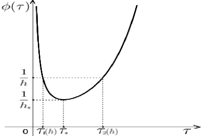
Figure 1: Function $\phi$

$\bullet$   The equation (2.3) is solvable if $h\leqslant h_{*}$ only, where $h_{*}:=\frac{1}{\phi(\tau_{*})}$. For $h<h_{*}$ it has two distinct roots $\tau_{1,2}(h):\,\tau_{1}(h)<\tau_{2}(h)$; for $h=h_{*}$ the roots coincide. For $h\to 0$ one has $\tau_{1}(h)\to 0$ and $\tau_{2}(h)\to\infty$, the relations

$$\lim\limits_{h\to 0}\frac{\tau_{1}(h)}{h}\,=\,1\,,\qquad\lim\limits_{h\to 0}h\,\frac{e^{\tau_{2}(h)}}{\tau_{2}(h)}\,=\,2$$ (2.5)

being valid.

$\bullet$    The function $\tau_{1}(h)$ defined for $0\leqslant h\leqslant h_{*}$ is invertible; the inverse function is

$$h\,=\,h(\tau_{1})\,\overset{(\ref{transcend eq})}{=}\,\frac{\tau_{1}}{{\rm ch}\tau_{1}}\,,\qquad 0\leqslant\tau_{1}\leqslant\tau_{*}\,.$$

For the latter, we have

$$\frac{dh}{d\tau_{1}}\,=\,\frac{1-\tau_{1}{\rm th}\tau_{1}}{{\rm ch}\tau_{1}}$$

that leads to

$$\frac{d\tau_{1}}{dh}\,=\,\frac{{\rm ch}\tau_{1}}{1-\tau_{1}{\rm th}\tau_{1}}\,,\qquad\lim\limits_{h\to h_{*}}\frac{d\tau_{1}}{dh}\,\overset{(\ref{eq for tau*})}{=}\,\infty\,.$$ (2.6)

In particular, the aforesaid shows that for $h\leqslant h_{*}$ the functional $S_{h}[y]$ possesses two extremals

$$y_{1,2}(x)\,\overset{(\ref{extr general})}{=}\,\frac{h}{\tau_{1,2}(h)}\,{\rm ch}\left[\frac{\tau_{1,2}(h)}{h}\,x\right]\,,\qquad-h\leqslant x\leqslant h\,,$$ (2.7)

which are distinct if $h<h_{*}$ and coincide if $h=h_{*}$. For $h>h_{*}$, the functional $S_{h}[y]$ does not possess extremals. On fig 2, the graphs of extremals are shown for a small, intermediate, and critical values of the distance $h$.

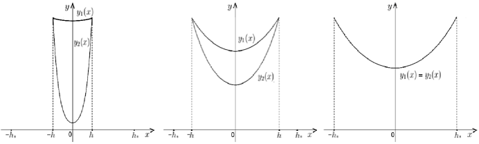
Figure 2: The extremals

Substituting (2.7) to (2.1), one gets the equalities

$$S_{h}\left[y_{1,2}\right]\,=\,2\pi\frac{h^{2}}{\tau_{1,2}(h)}+\pi\,\frac{h^{2}}{\tau_{1,2}^{2}(h)}\,{\rm sh}\,2\tau_{1,2}(h)\,,\qquad 0<h\leqslant h_{*}\,.$$ (2.8)

By them, with regard to (2.5), one easily derives the relations

$$\lim\limits_{h\to 0}S_{h}[y_{1}]\,=\,0\,,\qquad\lim\limits_{h\to 0}S_{h}[y_{2}]\,=\,2\pi\,.$$

Some additional analysis implies

$$S_{h}[y_{1}]\,<\,S_{h}[y_{2}]\,,\qquad 0<h<h_{*},$$ (2.9)

wheraes $S_{h_{*}}[y_{1}]=S_{h_{*}}[y_{2}]$ holds by coincidence of the extremals for $h=h_{*}$ (see fig 3).

Second variation

Testing the extremals on the presence of extremum, we use the Taylor representation

$$S_{h}[y+t\eta]\,\underset{t\,\sim\,0}{=}\,S_{h}[y]+t\delta S_{h}[y;h]+t^{2}\delta^{2}S_{h}[y;h]+t^{3}\delta^{3}S_{h}[y;h]+o(t^{3})$$ (2.10)

and, in particular, the second variation. Its general form at the extremals (2.1) is derived by the straightforward differentiation:

$$\delta^{2}S_{h}[y;\eta]:=\frac{1}{2!}\,\left[\frac{d^{2}}{dt^{2}}\,S_{h}[y+t\eta]\right]\bigg{|}_{t=0}\overset{(\ref{basic functional}),(\ref{extr general})}{=}\frac{1}{2C}\int_{-h}^{h}\frac{C^{2}{\eta^{\prime}}^{2}(x)-\eta^{2}(x)}{{\rm ch}^{2}\frac{x}{C}}\,dx\,,$$

where $\eta\in C^{1}[-h,h]$ is a test function, $\eta(-h)=\eta(h)=0$. Introducing a new variable $s=\frac{x}{C}$ and test function

$$\psi(s):=\frac{\eta(Cs)}{{\rm ch}s}\qquad(\,\text{so\, that}\,\,\,\,\eta(x)=\psi\left(\frac{x}{C}\right){\rm ch}\frac{x}{C}\,)\,,$$ (2.11)

and integrating by parts with regard to $\psi(-\tau)=\psi(\tau)=0$, after some simple calculation we get

$$\delta^{2}S_{h}[y;\eta]=\alpha\int_{-\tau}^{\tau}\left[{\psi^{\prime}}^{2}(s)-\frac{2}{{\rm ch}^{2}s}\,\psi^{2}(s)\right]\,ds\,,$$ (2.12)

where $\alpha={\rm const}>0$.

Let us consider the integral in (2.12) as a functional of $\psi$. For it, the corresponding Euler equation takes the form of the Sturm-Liouville equation

$$\psi^{\prime\prime}+\frac{2}{{\rm ch}^{2}s}\psi\,=\,0$$ (2.13)

with the soliton potential $q=\frac{2}{{\rm ch}^{2}s}$. We did not succeed to recognize, whether it appears in the given problem just by occasion, or there is a deeper reason for that.

We study the second variation by the use of the special solution to (2.13) of the form

$$\mu(s)\,:=\,1-s\,{\rm th}s\,.$$ (2.14)

It is distinguished by the conditions $\mu(0)=1$ and $\mu(-s)=\mu(s)$, has the ordinary roots $\tau=\mp\tau_{*}$ (see (2.4)), and is positive in the interval $(-\tau_{*},\tau_{*})$. Recall that, outside its roots, any solution to the equation $u^{\prime\prime}+qu=0$ satisfies the well-known Riccati equation

$$\left[\frac{u^{\prime}}{u}\right]^{\prime}+\left[\frac{u^{\prime}}{u}\right]^{2}=-q\,.$$

Applying this to the solution $\mu$, we have

$$\left[\frac{\mu^{\prime}}{\mu}\right]^{\prime}+\left[\frac{\mu^{\prime}}{\mu}\right]^{2}=-\frac{2}{{\rm ch}^{2}\tau}\,.$$ (2.15)

Therefore, for $|\tau|<\tau_{*}$ (outside the roots of $\mu$) the following transformations of the integral in (2.12) turn out to be quite correct:

$$\int_{-\tau}^{\tau}\left[{\psi^{\prime}}^{2}(s)-\frac{2}{{\rm ch}^{2}s}\,\psi^{2}(s)\right]\,ds\overset{(\ref{Riccati for mu})}{=}\int_{-\tau}^{\tau}\left\{{\psi^{\prime}}^{2}+\left[\left(\frac{\mu^{\prime}}{\mu}\right)^{\prime}+\left(\frac{\mu^{\prime}}{\mu}\right)^{2}\right]\,\psi^{2}\right\}\,ds\overset{(*)}{=}$$

$$=\int_{-\tau}^{\tau}\left[{\psi^{\prime}}^{2}-\frac{\mu^{\prime}}{\mu}\,\left(\psi^{2}\right)^{\prime}+\left(\frac{\mu^{\prime}}{\mu}\right)^{2}\,\psi^{2}\right]\,ds=\int_{-\tau}^{\tau}\left[{\psi^{\prime}}-\frac{\mu^{\prime}}{\mu}\,\psi\right]^{2}ds\,.$$

Integrating by parts in the equality $(*)$, one uses the boundary conditions $\psi(\mp\tau)=0$. The same conditions yield that $\frac{\psi}{\mu}$ is bounded as $|s|\leqslant\tau_{*}$, what enables one to justify the derivation also in the case $\tau=\tau_{*}$.

As a consequence, for the second variation (2.12) on any test function $\eta$, we have:

$$\delta^{2}S_{h}[y;\eta]=\beta\,\int_{-\tau}^{\tau}\left[{\psi^{\prime}}-\frac{\mu^{\prime}}{\mu}\,\psi\right]^{2}ds=\begin{cases}>0&\text{for}\,\,\,\tau<\tau_{*}\\ \geqslant 0&\text{for}\,\,\,\tau=\tau_{*}\end{cases},$$ (2.16)

the equality $\delta^{2}S_{h}[y;\eta]=0$ (for $\tau=\tau_{*}$) being valid only on the function $\eta$, which corresponds (in the meaning of (2.11)) to the function $\psi=c\mu$ with a constant $c\not=0$.

Extremal $y_{1}$

Fix an $h<h_{*}$; for it, the equality $\tau_{1}(h)<\tau_{*}$ holds. By the latter, the representation (2.16) is valid with $\tau<\tau_{*}$ that implies

$$\delta^{2}S_{h}[y_{1};\eta]\,>\,0$$

for any test function $\eta$. Consequently, on the extremal $y_{1}$ the functional $S_{h}[y]$ does attain a minimum. Its minimal value is determined by (2.8). As is seen from (2.9), this minimum is local (is not global).

Extremal $y_{2}$

For $h<h_{*}$, one has $\tau_{2}(h)>\tau_{*}$ and the representation (2.16) becomes invalid. Let us show that the variation $\delta^{2}S_{h}[y_{2};\eta]$ turns out to be sign-indefinite and takes negative values on appropriate $\eta$.

Consider the boundary value spectral problem

$$\psi^{\prime\prime}+\lambda\frac{2}{{\rm ch}^{2}s}\psi\,=\,0\,,\qquad-\tau<s<\tau$$ (2.17)

$$\psi(-\tau)\,=\,\psi(\tau)\,=\,0$$ (2.18)

for an inhomogeneous string with the density $\rho=\frac{2}{{\rm ch}^{2}s}$ and the fixed endpoints. Here $\tau$ is a parameter. Recall the well-known facts (see, e.g., [1]).

$\bullet$   The problem possesses the ordinary discrete spectrum $\{\lambda_{k}(\tau)\}_{k\geqslant 1}$:

$$0<\lambda_{1}(\tau)<\lambda_{2}(\tau)<\dots,\quad\lambda_{k}(\tau)\underset{k\to\infty}{\to}\infty\,,$$

whereas the corresponding eigenfunctions $\{\psi_{k}(\cdot\,;\tau)\}_{k\geqslant 1}$ constitute an orthogonal basis of the space $L_{2,\,\rho}(-\tau,\tau)$.

$\bullet$   The relation $\frac{d\lambda_{k}(\tau)}{d\tau}<0$ holds, so that the eigenvalues are the strictly monotonic decreasing functions of $\tau$.

$\bullet$   The first (minimal) eigenvalue is

$$\lambda_{1}(\tau)\,=\,\min\limits_{0\not=\psi\in H^{1}_{0}[-\tau,\tau]}\frac{\int_{-\tau}^{\tau}{\psi^{\prime}}^{2}(s)\,ds}{\int_{-\tau}^{\tau}\frac{2}{{\rm ch}^{2}s}\,\psi^{2}(s)\,ds}\,,$$ (2.19)

where $H^{1}_{0}[-\tau,\tau]:=\{y\,|\,\,y,y^{\prime}\in L_{2}(-\tau,\tau),\,y(\mp\tau)=0\}$ is the Sobolev space. For $\tau\to 0$ one has $\lambda_{1}(\tau)\to\infty$.

$\bullet$   The eigenfunction $\psi_{1}$ has no roots in $-\tau<s<\tau$. The functions $\psi_{k}$ of the numbers $k\geqslant 2$ do have the roots into this interval.

By the above mentioned facts, the behavior of the low bound of the string spectrun is the following. For $\tau\sim 0$, we have $\lambda_{1}(\tau)\gg 1$. As $\tau$ grows, the value of $\lambda_{1}(\tau)$ is decreasing, whereas for $\tau=\tau_{*}$ one has $\lambda_{1}(\tau_{*})=1$ and $\psi_{1}=c\mu$. Indeed, for $\tau=\tau_{*}$ the equation (2.13) possesses the solution $\psi=\mu$, which satisfies the conditions (2.18), i.e., is an eigenfunction of the string corresponding to $\lambda=1$. It is namely the first eigenfunction since $\mu$ has no roots into $(-\tau_{*},\tau_{*})$.

Further, for $\tau>\tau_{*}$, by monotonicity of the eigenvalues, we have $\lambda_{1}(\tau)<1$. Therefore, by (2.19), there is a function $\psi_{0}\in H^{1}_{0}[-\tau,\tau]$ satisfying

$$\frac{\int_{-\tau}^{\tau}{{\psi_{0}}^{\prime}}^{2}(s)\,ds}{\int_{-\tau}^{\tau}\frac{2}{{\rm ch}^{2}s}\,\psi_{0}^{2}(s)\,ds}\,<\,1$$

that is equivalent to

$$\int_{-\tau}^{\tau}\left[{{\psi_{0}}^{\prime}}^{2}(s)-\frac{2}{{\rm ch}^{2}s}\,{\psi_{0}}^{2}(s)\right]\,ds\,<\,0\,.$$

Therefore, for the function $\eta_{0}$ related with $\psi_{0}$ via the relation (2.11), by virtue of (2.12) one has:

$$\delta^{2}S_{h}[y_{2};\eta_{0}]\,<\,0\,.$$

Hence, the extremal $y_{2}$ provides no extremum to the functional $S_{h}[y]$.

Critical case

The previous considerations deal with the case $h<h_{*}$. Now, let $h=h_{*}$, so that the extremals do coincide:

$$y_{1}(x)=y_{2}(x)\overset{(\ref{extremals y 1,2})}{=}\frac{h_{*}}{\tau_{*}}\,{\rm ch}\left[\frac{\tau_{*}}{h_{*}}\,x\right]\,=:\,y_{*}(x)\,,\qquad-h_{*}\leqslant x\leqslant h_{*}\,.$$

Let us show that there is no extremum at $y_{*}$. Recall that the function $\mu$ is defined in (2.14).

Find the variations of the functional $S_{h_{*}}[y]$, choosing

$$\eta_{*}(x)\overset{(\ref{test function})}{=}\,\mu\left(\frac{\tau_{*}}{h_{*}}\,x\right){\rm ch}\left[\frac{\tau_{*}}{h_{*}}\,x\right]$$

as a test function. By the choice, we have $\delta S_{h_{*}}[y_{*};\eta_{*}]=0$ $\delta^{2}S_{h_{*}}[y_{*};\eta_{*}]\overset{(\ref{Repres delta^2 S})}{=}0$. Let us find the third variation. As one can easily verify, on the arbitrary element and test function it is of the form

$$\delta^{3}S_{h}[y;\eta]:=\frac{1}{3!}\,\left[\frac{d^{3}}{dt^{3}}\,S_{h}[y+t\eta]\right]\bigg{|}_{t=0}=$$

$$=\pi\int_{-h}^{h}\frac{{\eta^{\prime}}^{2}(x)}{\left(1+{y^{\prime}}^{2}(x)\right)^{\frac{3}{2}}}\left[\eta(x)-\frac{y(x)y^{\prime}(x)\eta^{\prime}(x)}{1+{y^{\prime}}^{2}(x)}\right]dx\,.$$

Taking $h=h_{*},\,y=y_{*}$ $\eta=\eta_{*}$, the simple calculation provides:

$$\delta^{3}S_{h_{*}}[y_{*};\eta_{*}]=\frac{2\pi\tau_{*}^{4}}{3h_{*}}\,\not=\,0\,.$$

By (2.10), we have $S_{h_{*}}[y_{*}+th_{*}]\,\underset{t\,\sim\,0}{=}\,\gamma\,t^{3}+o(t^{3})$ $\gamma\not=0$ that certifies the absence of extremum.

3 Comments

On the Goldschmidt condition

For $h>h_{*}$, the functional (1.1) with the conditions (1.2) does not have extremals at all. In [2] (chapter 17, section 2), this fact is accomplished with the following qualitative explanation.

As $h$ grows, the area o the film is growing. For sufficiently big $h$, by energy reasons, it turns out to be more profitable for the film to fill the both of the rings separately and, so, take the total area $\pi 1^{2}+\pi 1^{2}=2\pi$. By this, the film breaks, whereas the critical area value turns out to be $2\pi$, which is declared as the Goldschmidt break condition.

The given explanation is incorrect . Defining the ‘Goldschmidt constant’ $h_{G}$ as the solution of the equation $S_{h}[y_{1}]=2\pi$ (with respect to $h$), it is easy to recognize that it is solvable and

$$0.5277...=h_{G}<h_{*}=0.6627...\,,$$

so that the corresponding extremal $y_{1}$ does exist and describes a stable pre-critical shape of the film: see fig 3.

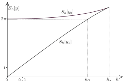
Figure 3:

Probably, the incorrect explanation is just a result of confusion. In the first exercise at the end of the section (page 689), the reader is proposed ‘to find such a value of $h$ that the rotation surface area is equal to the total area of the end rings’.

Physical considerations

Is the value $h=h_{*}$ distinguished from a physical viewpoint? Bellow we propose a variant of the answer on this question.

Let $h<h_{*}$ and the film be of the shape described by the extremal $y_{1}$. Contacting with the rings, the film influences on them by the surface stretch forces, the rings being attracted with each other. As the distance between them grows, the system accumulates a potential energy. In the framework of the model under consideration, one can assume the potential energy of the stretch forces to be proportional to the film area $S_{h}[y_{1}]$. The derivative

$$-\,\frac{dS_{h}[y_{1}]}{dh}=:F(h)$$

may be naturally interpreted as a force of the rings attraction. Let us find its value.

Denoting $R(\tau):=\frac{2}{\tau}+\frac{{\rm sh}2\tau}{\tau^{2}}\,,$ we have $S_{h}[y_{1}]\,\overset{(\ref{S[y 1,2]})}{=}\,\pi h^{2}R(\tau_{1}(h))$ that follows to

$$F(h)=-\,2\pi hR(\tau_{1}(h))-\pi h^{2}R^{\prime}(\tau_{1}(h))\tau_{1}^{\prime}(h)\,.$$

Implementing the differentiation in the right hand side, after the simple transformations with regard to the first of the equalities (2.6), we get

$$F(h)\,=\,-\,4\pi\,\frac{h}{\tau_{1}(h)}\,.$$

Differentiating one more time, we arrive at the relations

$$F^{\prime}(h)\,=\,-\,4\pi\,\frac{\tau_{1}(h)-h\tau_{1}^{\prime}(h)}{\tau_{1}^{2}(h)}\,\overset{(\ref{dtau/dh=infty})}{\quad\,\,\underset{h\to h_{*}}{\to}\infty}\,.$$

Such a behavior motivates to regard the value $h=h_{*}$ as critical: one may assume that it is the infinite velocity of the force growing, which leads to the break of the film, and forbids its existence for $h>h_{*}$.

References

- [1] F.V.Atkinson. Discrete and continuous boundary problems. Academic Press, New-York and London, 1964.
- [2] G.Arfken. Mathematical Methods for Physicists. Academic Press, New-York and London, 1966.
-
[3]
V.S.Buslaev.
Calculus of Variations.
Leningrad State University,
Leningrad, 1980. (in Russian)
Translated by M.I.Belishev