Global flow of the Higgs potential in a Yukawa model
Abstract
We study the renormalization flow of the Higgs potential as a function of both field amplitude and energy scale. This overcomes limitations of conventional techniques that rely, e.g., on an identification of field amplitude and RG scale, or on local field expansions. Using a Higgs-Yukawa model with discrete chiral symmetry as an example, our global flows in field space clarify the origin of possible meta-stabilities, the fate of the pseudo-stable phase, and provide new information about the renormalization of the tunnel barrier. Our results confirm the relaxation of the lower bound for the Higgs mass in the presence of more general microscopic interactions (higher-dimensional operators) to a high quantitative accuracy.
I Introduction
The discovery of a Higgs boson at the LHC Aad et al. (2012); Chatrchyan et al. (2012) completed the search for the building blocks of the standard model of particle physics. While the mass of the Higgs boson is in principle a free parameter of the standard model, it has long been known that it is not necessarily an arbitrary parameter. For instance, assuming that the description of fundamental physics in terms of standard-model degrees of freedom is valid at a high energy scale and that the theory is sufficiently weakly coupled, the range of possible Higgs boson masses is restricted by a finite range, the so-called infrared (IR) window Maiani et al. (1978); Krasnikov (1978); Lindner (1986); Wetterich (1987); Altarelli and Isidori (1994); Schrempp and Wimmer (1996); Hambye and Riesselmann (1997). The fact that this IR window shrinks for increasing can be traced back to the fixed-point structure of the RG flow Wetterich (1987, 1981) which connects the mass of the Higgs boson to that of the heaviest quark.111This implies that the results of the present paper could equally well be rephrased in terms of bounds on the top mass. This might even be the more relevant viewpoint Bezrukov and Shaposhnikov (2015), as the top mass is presently known less precisely. However, we stick to the “Higgs boson mass” perspective in order to conform with a larger part of the literature.
The edges of the IR window Krive and Linde (1976); Hung (1979); Linde (1980); Cabibbo et al. (1979); Politzer and Wolfram (1979); Kuti et al. (1988); Sher (1989); Hasenfratz et al. (1987); Luscher and Weisz (1989); Lindner et al. (1989); Ford et al. (1993); Heller et al. (1993); Arnold (1989); Sher (1993); Altarelli and Isidori (1994); Casas et al. (1995); Espinosa and Quiros (1995); Bergerhoff et al. (1999); Isidori et al. (2001); Ellis et al. (2009); Holthausen et al. (2012); Elias-Miro et al. (2012); Degrassi et al. (2012); Alekhin et al. (2012); Masina (2013); Buttazzo et al. (2013); Gabrielli et al. (2014); Bednyakov et al. (2015), i.e., the upper and lower admissible values, for the Higgs mass are actually not sharply defined, but depend on a number of additional assumptions. This is most obvious for the upper “triviality bound”, as the Higgs sector becomes strongly coupled at high scales for large values of the Higgs mass. Perturbative estimates of this bound, e.g., depend on an ad hoc choice of coupling value up to which perturbation theory is trusted. Nonperturbative methods have shown that this upper bound relaxes considerably if one allows the system to start microscopically with a strong Higgs self-coupling Gies et al. (2014); Gies and Sondenheimer (2015).
As is less well appreciated, a similar fuzziness also holds for the lower edge of the IR window on which we concentrate in the present work. This indeterminacy arises from the (implicit) assumptions imposed on the precise form of the microscopic theory at the high scale . For instance, by considering only renormalizable operators in conventional perturbative estimates of the lower bound, the couplings of all higher-order operators are implicitly chosen to vanish at the high scale . Strictly speaking, this corresponds to fixing infinitely many further parameters, in addition to the parameters of the standard model.222This statement holds for any finite value of . If the limit could be taken, e.g., at an asymptotically free or asymptotically safe fixed point, all these parameters would be predictions of the theory. Whether the standard model could have this property is not fully understood, hence presumably remains a finite though unknown parameter of the model.
By contrast, if one defines the standard model more agnostically in terms of its symmetries, field content and measured IR parameters, the microscopic interactions quantified by the bare action at the high scale remains largely unspecified. It can contain infinitely many operators and corresponding coupling constants which would be computable if the underlying theory was known. It is reasonable to assume that these couplings if measured in units of the scale are of order . Still, an even more strongly coupled UV regime is not excluded by observation. The fact that the perturbative description of electroweak collider data works so well indicates that colliders so far probe a regime where Nature is close to the Gaußian fixed point of the renormalization group (RG). Here, power-counting arguments hold and higher-dimensional operators are irrelevant, exerting a negligible influence on IR observables. In turn, the IR observables dominantly constrain only the marginal and relevant (renormalizable) operators of the bare action and put hardly any bound on the irrelevant couplings.
In a series of works, it has recently been shown that these unconstrained higher-dimensional operators in fact can relax the lower edge of the IR window, i.e., can lower the lower (stability) bound on the Higgs mass without introducing metastability Gies et al. (2014); Gies and Sondenheimer (2015); Eichhorn et al. (2015). Comparatively simple modifications of the bare action, e.g., in terms of a dimension-six operator at the Planck scale can lower the lower mass bound by GeV, while preserving absolute stability on all scales Eichhorn et al. (2015). The mechanism behind this relaxation of the lower edge has two aspects: first, negative couplings of renormalizable operators which seem to introduce an instability from a perturbative viewpoint can still be associated with a fully stable potential in the presence of the higher-dimensional operators. Second, the higher-dimensional operators take influence on the running of the renormalizable part over a range of scales thus modifying the approach to the perturbative region while leaving the IR region itself intact as addressed by perturbation theory.
These results can already be observed in a simple mean-field study (large- limit) as well as in extended mean-field approximation (1/ corrections), but unfold more comprehensively in a controlled nonperturbative study using the functional RG. They have been confirmed by lattice simulations in the range of scales accessible to current lattice sizes Hegde et al. (2014); Chu et al. (2015, 2014); Akerlund and de Forcrand (2015). Recent functional RG studies also including higher-order fermionic operators have shown the same features Eichhorn and Scherer (2014); Jakovac et al. (2015a, b); for further studies of higher-dimensional operators in this context, see, e.g., Datta et al. (1996); Barbieri and Strumia (1999); Grzadkowski and Wudka (2002); Burgess et al. (2002); Barger et al. (2003); Blum et al. (2015).
While controlled quantitative results have so far been obtained for a small class of operators represented by simple low-order polynomials of the field, a possible metastable regime with competing vacua has not been explored so far.
The present work is devoted to a first step in this direction, namely to study the full functional renormalization of the Higgs effective potential as a function of both field amplitude and RG scale. This is facilitated by the development of pseudo-spectral methods for functional flows Borchardt and Knorr (2015, ). If applied to the fully stable regimes studied before, our results confirm the lowering of the Higgs mass bounds to a high accuracy. In addition, the full potential solver allows to address the fate of the RG flow in potential metastable regimes and the renormalization of the tunnel barrier.
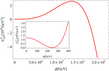
Our present study is performed within a simple Higgs-Yukawa model with a discrete chiral symmetry, which has proved useful for addressing the qualitative properties of the IR window. Our main results are read off from the properties of the Higgs effective potential as a function of field amplitude and RG scale . A first illustration for such a fully stable flow is shown in Fig. 1, where the dimensionless potential is depicted as a function of the dimensionless field amplitude for various values of ranging from the UV towards the IR (blue to black) where a vacuum expectation value has developed.

The paper is organized as follows: in Sect. II, we introduce our toy model and briefly summarize some recent results which are of relevance for our present study. Section III is devoted to an extensive mean-field study, for the first time also including the meta-stable regime. Here, we also clarify the fate of a recently discovered pseudo-stable phase Eichhorn et al. (2015) and discuss the connection with the effective single-scale potential obtained from conventional perturbative constructions. In Sect. IV we investigate the full RG flow of the entire scalar potential by means of the functional RG. We compare the local behavior around the electroweak minimum as well as the global behavior with the results obtained by polynomial expansion of the potential and the mean-field estimates. While we still span the bare potential in terms of a few polynomial operators in this work, the techniques used here will facilitate future studies of general classes of bare actions.
II Higgs-Yukawa model with discrete symmetry
II.1 The model
All mechanisms relevant for the present work can already be studied in a simple Higgs-Yukawa model corresponding to the reduction of the standard model to the top quark with the largest Yukawa coupling, and a real scalar Higgs degree of freedom . The classical euclidean action of this model is given by:
| (1) |
The model features a discrete chiral symmetry, , , mimicking the global part of the electroweak symmetry group, and protecting the fermion against acquiring a mass term. No massless Goldstone bosons appear after spontaneous symmetry breaking as the symmetry is discrete. Hence, the particle spectrum is gapped in the broken phase as in the standard model. This toy model was intensively discussed in the context of stability of the effective potential in the literature, e.g., Holland and Kuti (2004); Holland (2005); Branchina and Faivre (2005); Gies et al. (2014); Krajewski and Lalak (2015).
In order to make semi-quantitative contact with the standard model, we impose Coleman-Weinberg renormalization conditions Coleman and Weinberg (1973) on the effective potential obtained after integrating out all fluctuations down to the IR,
| (2) |
where denotes the (renormalized) field value at the minimum of the potential333For the plots below, the physically irrelevant zero point is chosen such that either or depending on numerical convenience., and all couplings are also considered to be renormalized at a suitable renormalization point , e.g., . In the present work, we choose for the observable parameters: GeV for the top mass, and GeV. The Higgs mass then is treated as a function of the cutoff and a functional of the bare action, .
Despite this apparent physical fixing, the simplified model, of course, deviates quantitatively from the standard model in essential aspects: for instance, whereas the center of the IR window for the Higgs mass is near GeV for a Planck scale cutoff in the standard model Buttazzo et al. (2013), it is near GeV for the present simple model at high energy scales Eichhorn and Scherer (2014) mainly due to the absence of the gauge sectors.
II.2 Perturbative effective single-scale potential
In order to make contact with the conventional perturbative treatment, we briefly sketch the standard line of argument to obtain an estimate of the effective potential. For simplicity, we consider only the one-loop level. Perturbatively, only the renormalizable operators of the bare potential are considered,
| (3) |
featuring the bare mass parameter and bare coupling . The estimate for the effective potential is based on the function for the renormalized running coupling ,
| (4) |
depending as well on the renormalized running Yukawa coupling . For the present line of argument, it suffices to ignore the running of (it will be fully included in our detailed studies later). The discussion can even be simplified further by noting that the -terms in Eq. (4) are small compared to the term for small Higgs masses and large top masses. In this limit which corresponds to ignoring scalar fluctuations, the integration of the function yields
| (5) |
with denoting the renormalization point for .
The conventional perturbative estimate of the effective potential is then inspired by the Coleman-Weinberg form of the effective potential Coleman and Weinberg (1973). One assumes that the effective potential is well approximated by identifying the dependence of the integrated scalar self-coupling on the RG scale with the scalar field itself, . We emphasize, that the identification mixes momentum scale information with the field amplitude. In general, the full effective action in field theory would provide separate information about the two scales which need not be the same. By this identification, we obtain a single-scale potential which in our simple approximation reads
| (6) |
Imposing the renormalization conditions (2) together with the choice , we can write the single-scale potential as
| (7) |
Note also, that the bare potential (3) remains completely unspecified in this derivation. The implicit use of only renormalizable operators together with the limit permitted by perturbative renormalizability seems to suggest that the details of the bare potential are irrelevant.
Clearly, this single-scale potential develops an instability for large Yukawa couplings, i.e., large . For the present choice of parameters, the instability occurs at a scale of GeV in our toy model, see Fig. 2. This instability is related to the running of , which turns negative at sufficiently large , cf. Eq. (5).
In the full standard model, the corresponding instability scale is of order GeV. Though current state-of-the-art calculations Buttazzo et al. (2013); Degrassi et al. (2012); Bednyakov et al. (2015) determine the single-scale potential to NNLO precision, including two-loop threshold corrections, and self-consistent resummations Andreassen et al. (2014, 2015), the present rather cartoon-like presentation in a toy model still captures the essence of the origin of the instability occurring in the perturbative estimate of the single-scale potential.
A qualitative difference arises in the standard model from the electroweak gauge fluctuations, which render the coupling positive again at even higher scales such that the single-scale potential becomes bounded from below and a second minimum arises beyond the Planck scale which turns out to be the global one. Therefore, the absolute instability of the single-scale potential is a particularity of our model. Below, this will actually be useful to make one of our main points more transparent.
III Mean-field effective potential and stability
In the following, we use mean-field methods to study the effective potential. We stick to the same simplifications as before, ignoring bosonic fluctuations and the running of the Yukawa coupling, but keep track of all scales involved, the momentum scale of fluctuations , the field amplitude and the UV cutoff scale . Parts of this discussion follows Gies et al. (2014); Gies and Sondenheimer (2015), where also more technical details can be found. Here, we focus on the new aspects arising for un-/metastable scenarios.
III.1 Mean-field potential
With these prerequisites, the mean-field potential is directly related to the fermion determinant. More precisely, working with an explicit UV cutoff and an IR regulator scale , the mean-field potential reads,
| (8) |
where denotes the spacetime volume, and irrelevant field independent constants are ignored. If we introduced fermion flavors, the mean-field potential would become exact in the limit . The notation indicates that the determinant is regularized and includes momentum modes in the range . The result is regularization dependent. As long as we do not send , this dependence is physical and can be viewed as a model for the details of the embedding into a more fundamental underlying UV complete theory. For a close contact with later sections, we use a piece-wise linear regulator familiar from functional RG studies Litim (2000, 2001); we emphasize that all conclusions remain the same also for a sharp momentum cutoff, propertime or zeta-function regularization, see Gies and Sondenheimer (2015). We obtain,
| (9) |
which makes all scale dependencies explicit. By varying the RG scale , we can observe how the mean-field effective potential as a full function of the field amplitude ,
| (10) |
is built up from fermionic fluctuations renormalizing the bare potential while running from to .
Apart from the induced mass term , the whole interaction part of the determinant (2nd line of Eq. (10)) is positive. The bare mass term can now be fixed by the renormalization condition , fixing the Fermi scale,
| (11) |
Inserting Eq. (11) into Eq. (10) yields a globally stable effective potential for any value of the UV cutoff and any admissible non-negative value of the bare coupling , cf. solid black line in Fig. 3. It is important to stress that a bare potential of quartic type, Eq. (3), with negative would be inconsistent right from the beginning, as the functional integral over the scalar field would be ill-defined.
For completeness of the presentation, we recall that the mass of the scalar particle now becomes a function of the cutoff and , cf. Gies et al. (2014); Gies and Sondenheimer (2015),
| (12) |
This demonstrates that a lower bound for the Higgs mass is obtained by the physical restriction that the bare potential of -type at a given UV cutoff must be bounded from below, i.e., . Thus, the lower bound (lower edge of the IR window) is given by for this class of bare potentials. This way of determining the lower bound has been suggested in Holland and Kuti (2004); Holland (2005), and has been used in full non-perturbative lattice simulations Fodor et al. (2007); Gerhold and Jansen (2007a, b, 2009). Generically, one observes a strong quantitative agreement with mean-field theory for this lower bound. In this fashion, strong constraints on the existence of a heavy fourth generation arise Gerhold et al. (2011); Bulava et al. (2013a, b); Djouadi and Lenz (2012).
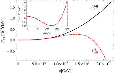
For the purpose of the present work, we reverse the line of argument: for a given Higgs mass of, say GeV, this implies that a maximal scale of UV extension is obtained. Choosing the minimal admissible value a cutoff of GeV is obtained by writing . For larger values of the UV cutoff, no physical (mean-field) RG trajectory can be found that connects an admissible bounded bare potential to an IR Higgs mass of GeV. As long as , the bare potential as well as the effective potential do not exhibit an instability. Figure 3 shows a comparison between the mean-field potential (solid/black line) where the cutoff is kept finite and the single-scale potential (red/dashed line) where the cutoff has implicitly been sent to infinity. The single-scale potential approximation starts to break down for field amplitudes, where , i.e., where terms which are dropped in the implicit limit are actually sizable.
It is, of course, possible to reduce the multi-scale mean-field potential to the single-scale potential. First, we blindly enforce all renormalization conditions. In particular the first condition in Eq. (2) for large cutoffs implies
| (13) |
Inserting Eq. (13) and Eq. (11) into the mean-field effective potential finally leads to a potential with the requested minimum at and Higgs mass of by construction. The cutoff remains still a free parameter. In the naive large cutoff limit, we obtain
For a cutoff larger than the critical value , the potential develops an instability and rapidly approaches the single-scale potential, see Fig. 4. For GeV, the difference between the mean-field effective potential with a finite cutoff and the single-scale potential with implicit limit becomes very small. Taking the naive limit , the single-scale potential (7) is obtained as expected.
We emphasize that the consistency condition that the bare potential should be bounded from below for a well-defined generating functional is no longer fulfilled for all . This can be directly read off from expression (13): has to be chosen negative for , and thus already the bare potential is unstable. At this point, we conclude that the apparent instability of the single-scale potential appears due to an inconsistent UV boundary condition for the theory. As long as the consistency condition is fulfilled, no instability can be found within the class of quartic bare potentials.
III.2 Generalized bare potentials
As already emphasized in Gies et al. (2014); Gies and Sondenheimer (2015); Eichhorn et al. (2015), these observations do not imply that in- or metastabilities are completely excluded. Whether or not an in-/metastability occurs is not a matter of the fermionic fluctuations but has to be seeded by the microscopic underlying theory. A specific example from string phenomenology is given in Hebecker et al. (2013).
From the perspective of the standard model as an effective field theory, the embedding into a UV complete theory is parametrized by the bare action at the cutoff . Of course, the bare action is expected to host all operators compatible with the symmetry with couplings of order in units of the cutoff .
In the following, we consider the simplest extension of the bare potential by including a higher-dimensional operator as an example,
| (14) |
Within the same mean-field approximation as used before, we can straightforwardly compute the mass of the Higgs boson in our model as a function of and the parameters and , cf. Eq. (12),
| (15) |
It is obvious that the previous lower bound of Eq. (12) can be relaxed by a negative value for , while a positive can stabilize the bare potential. For small negative and sufficiently large the effective potential as well as the potential at intermediate scales are globally stable and have a unique minimum. In this regime, it is easily possible to obtain Higgs masses below the perturbative lower bound, i.e., decrease the edge of the IR window.
For even smaller , i.e., larger absolute values of a negative , the effective potential starts to develop a second minimum towards lower RG scales and becomes metastable, while the bare potential is still stable. For even smaller values of , also the bare potential can become metastable.
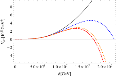
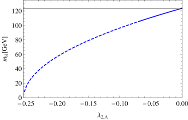
For an illustration, let us assume a fixed cutoff GeV. Within the class of quartic bare potentials (3), the lowest Higgs mass according to Eq. (12) is given by GeV for . Stabilizing the more general class of bare potentials (14) with a fixed value of , we can choose negative values of , yielding also smaller values of the Higgs mass, see Fig. 5. The resulting mean-field potentials are stable with a unique (electroweak) minimum on all scales (blue solid line) until we reach a value for the bare quartic coupling of . For even smaller values of , a second minimum arises in the course of the mean-field flow, while the bare potential still has a unique minimum. This second minimum is a local minimum only for a small range of values, . For , the second minimum becomes the global one (blue dashed line), which renders the electroweak minimum in the effective potential metastable. Within this regime of metastability, the Higgs mass can be made arbitrarily small by a suitable choice of parameters even without any metastability in the bare potential.
It is important to emphasize that the metastability observed here in this model is a consequence of the shape of the bare potential encoded in both renormalizable and non-renormalizable operators. In the present model, this metastability remains invisible in the perturbatively estimated single-scale potential which would predict complete instability. We conclude that metastability properties of the model can only be reliably calculated if the bare potential at a UV scale is known. The single-scale potential is not sufficient as a matter of principle.
In the present model, this conclusion becomes obvious as the single-scale potential does not even exhibit a metastable region. This is different from the standard model, where the single-scale potential itself predicts metastability for light Higgs masses, as the single-scale potential is stabilized by electroweak fluctuations again at high field amplitudes. Still, the same conclusion about the reliability of the metastability estimate of the single-scale potential holds as for the simple model.
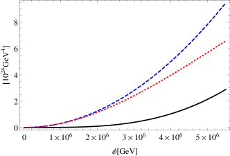
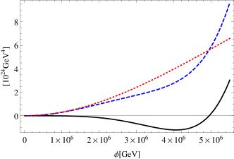
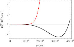
The fact that the metastability in the effective potential is seeded in the bare potential is illustrated in Fig. 6. Here, the effective mean-field potential (black solid line) is shown as the difference between the bare potential (blue dashed line) and the absolute value of the fermion determinant (red dotted line). The left panel depicts the case with stable bare as well as effective potential (initial parameters: GeV, , ). By contrast, the right panel shows the case where a second minimum arises in the effective potential (initial parameters: GeV, , ). One clearly sees how the modified structure of the generalized bare potential with a negative is responsible for the second minimum at large scales besides the electroweak one (the latter at GeV is hardly visible on the scales of the plot). We emphasize again that there is no possibility for the mean-field potential to develop a second minimum for the case of quartic bare potentials because the bare potential always exceeds the fermion determinant.
With the full mean-field potential at hand, we can also clarify the nature of the pseudo-stable phase observed in a polynomial expansion of the effective potential in Eichhorn et al. (2015). In this approximation, RG flows were observed that start at with a globally stable bare potential, then run trough a metastable regime with two minima and finally end up in the IR with one stable minimum at the Fermi scale. In the same spirit, we now expand the mean-field effective average potential (9) around the minimum at the origin and follow its flow in comparison with the flow of the full mean-field effective potential. This is depicted in Fig. 7. Indeed, the potential approximated by a polynomial expansion shows the same pseudo-stable behavior as observed in Eichhorn et al. (2015). A second minimum appears but disappears again after a short RG time. The polynomial expansion thus looks stable again in the IR. This is in contrast to the full mean-field potential where the second minimum survives the RG flow towards the IR. We conclude that the pseudo-stable phase is an artifact of the finite convergence radius of the polynomial expansion. The global effective mean-field potential exhibits a metastability also in this phase.
IV Nonperturbative flow of the scalar potential
IV.1 Functional renormalization group
While the mean-field approximation is highly convenient for first analytically controllable estimates, we have to go beyond for quantitative accuracy. The functional RG is an ideal tool for this task, as it resums large classes of higher-order diagrams, automatically accounts for threshold corrections and provides information about the global RG flow of the effective potential, i.e., all relevant scales can be studied independently. We use the Wetterich equation Wetterich (1993) in order to compute the RG flow of the effective action ,
| (16) |
The solution to this equation interpolates between the bare action and the full effective action that accounts for all quantum fluctuations. The regulator function implements the shell-by-shell integration at the momentum scale . denotes the Hessian of the effective average action with respect to the fields in the theory, . For detailed reviews see, Berges et al. (2002); Pawlowski (2007); Gies (2012); Delamotte (2012); Braun (2012).
We solve the Wetterich equation within a systematic derivative expansion of the action at next-to-leading order,
| (17) |
The Wetterich equation provides flow equations for the potential, the Yukawa coupling, and the wave function renormalizations for the fields and . The latter can be summarized by the anomalous dimensions of the fields,
| (18) |
In Eq. (17), we have introduced the unrenormalized scalar field , which is related to the renormalized field by . At mean-field level, the distinction is irrelevant as . In terms of dimensionless renormalized quantities,
| (19) | |||||
| (20) |
the nonperturbative flow equations in agreement with Gies and Scherer (2010); Gies et al. (2014); Gies and Sondenheimer (2015) read in spacetime dimensions
| (21) | ||||
| (22) | ||||
| (23) | ||||
| (24) |
where primes denotes derivatives with respect to . Here, we extract the flow of the Yukawa coupling and the anomalous dimensions at the (running) minimum of the potential ; see Vacca and Zambelli (2015) for an extended flow in the Yukawa sector. The threshold functions and encode the decoupling of massive modes. Evaluated for a piece-wise linear regulator function Litim (2000, 2001), these are listed, for instance, in Gies et al. (2014). Of course, the perturbative functions can be recovered from these nonperturbative flow equations by neglecting resummation and threshold effects. The flow equation also contains mean-field theory as a simple limit: ignoring the anomalous dimensions as well as the flow of the Yukawa coupling, and dropping the bosonic fluctuations in Eq. (21), the integration of the potential precisely yields the mean-field potential (9). Hence, all known limits are unified in the functional RG framework which we can now use to go beyond the perturbative/mean-field studies.
Previous work on Higgs boson mass bounds has solved the potential flow by means of a polynomial expansion Gies et al. (2014); Gies and Sondenheimer (2015); Jakovac et al. (2015a, b) about the flowing minimum. More concretely,
| (25) |
approximate the potential by a polynomial of degree in the symmetric (SYM) or symmetry-broken (SSB) regime. For the present problem, the quality of this expansion has been confirmed for potentials Gies et al. (2014) with a single minimum at any given scale. As the example of the seeming pseudo-stable phase above has shown, a proper description of metastability doubtlessly requires a PDE solver for the RG flow of the full potential (21) as a function of both and .
Solvers for such types of Yukawa systems have been successfully developed and applied in various functional RG studies from low-energy QCD models Bohr et al. (2001); Herbst et al. (2013), critical phenomena Adams et al. (1995); Hofling et al. (2002); Bonanno and Zappala (2001) to ultracold-gas systems Boettcher et al. (2015). The particular difficulty in the present case arises from the necessity to run the RG over many orders of magnitude in the presence of a relevant operator of canonical dimension 2. This requires substantial precision.
Another challenge is the approach to convexity which is expected to hold for the full effective potential O’Raifeartaigh et al. (1986); Litim et al. (2006), but is spoiled by both the perturbative single-scale potential as well as the mean-field approximation. Whereas the approach to convexity is less interesting for the case of a single minimum, it may become essential for metastable scenarios as the tunneling lifetime depends on the shape of the manifestly non-convex tunnel barrier.
IV.2 Pseudo-spectral flows
In general, the derivative expansion of the functional RG results in a system of coupled partial differential equations (PDEs). In the present case, we have to deal with one such PDE (21) coupled to an ODE (22) and two algebraic equations (23) and (24).
In order to obtain global information with high accuracy, we advocate pseudo-spectral methods Boyd (2000) which span the solutions in terms of global basis functions of high polynomial (or rational) degree. Under mild analyticity assumptions, the convergence to the exact result is exponential Boyd (2000). In particular in comparison with finite difference methods, pseudo-spectral methods are memory minimizing, as a certain accuracy requires only a comparatively small number of grid points.
In the following, we briefly sketch our methods; for more details, see Borchardt and Knorr . It is worth mentioning that pseudo-spectral methods have already successfully been applied to various problems in physics in general Robson and Prytz (1993); for first applications in the context of the functional RG, see Fischer and Gies (2004); Gneiting . The present code development is based on a highly accurate pseudo-spectral solver for computing global fixed-point solutions within the functional RG Borchardt and Knorr (2015).
In principle, pseudo-spectral methods include any kind of basis function system. In the present work, we use Chebyshev polynomials of the first kind. Boundary effects can be controlled since the polynomials are defined on a finite interval. The behavior of higher-order coefficients provides an error estimate of the absolute remainder of the solution. As a main advantage also in practice, function values, derivatives, and integrals of the objective function are easily accessible from the Chebyshev coefficients by means of recursive algorithms yielding a high precision calculation.
We apply pseudo-spectral methods in both the field and the RG time direction. For this, we subdivide the time interval into patches, apply a Newton-Raphson iteration to each patch, and solve for the coefficients. For minimizing the number of coefficients and increasing the resolution in physically interesting regions, we use multiple domains in field direction. All these patches are connected by additionally demanding matching conditions for the objective function and a sufficient number of its derivatives. The Newton-Raphson iteration provides an error estimate for the solution of the equations.
As a result, this method is stable over many orders of magnitude in . This enables us to choose high UV cutoffs. This choice is solely restricted by the number of digits needed for tuning the IR quantities. As the flow of the present problem includes a scalar mass parameter with canonical scaling of dimension 2, we need to tune approximately twice as many digits as the number of orders of magnitude between the UV scale and the Fermi scale. All full potential computations have been done with long double. Thus, we restricted ourselves to a maximal UV cutoff of GeV for the full potential calculation. In principle, higher values for are straightforwardly accessible by using a higher accuracy for the floating-point arithmetics.
IV.3 Higgs mass bounds
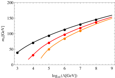
As a first benchmark, we perform a comparison to local polynomial solutions of the flow equation. For this, we compute Higgs masses for different initial values for the flow equations over a large range of cutoff values. In Fig. 8, we depict the resulting IR Higgs mass as a function of the UV cutoff : for the restricted class of bare potentials, the black data shows the resulting lowest possible Higgs mass, i.e., the conventional lower bound for . Examples within the class of generalized bare potentials that lead to a relaxation of the lower bound are shown in red (, ) and orange (, ). The solid lines mark the Higgs masses computed within the polynomial truncation, and filled circles indicate the Higgs masses resulting from the pseudo-spectral full potential computation of this work. The black and red line agree with the results of Gies et al. (2014), and illustrate the relaxation of the conventional lower bound by higher-dimensional operators. The orange data corresponds to a potential that develops a metastability (i.e., seems pseudo-stable in the polynomial expansion). For all cases, the pseudo-spectral data lies perfectly on top of the polynomial results. The full numerical PDE solution thus provides a strong confirmation that the polynomial expansion is suitable for extracting local information such as the Higgs mass ( curvature of the potential at ).
IV.4 Global flows
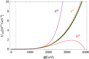
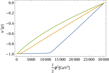
Let us start with a closer look at the global behavior of the flow for the class of the bare potentials. Obviously, the polynomial truncation lacks in describing the asymptotic behavior of the potential which can be seen in Fig. 9. This is not surprising since the flow equations suggest the asymptotic behavior to be that of the UV potential because fluctuations for large field amplitudes are suppressed. By contrast, the asymptotic behavior of the polynomial expansion by construction is fixed to the highest power of the field which is taken into account in the truncation, . These higher order couplings are generated during the RG flow, even if the bare potential is of type. Therefore, considering only terms up to , (accidentally) displays the asymptotic behavior best.
Naively, the polynomial truncation up to sixth order in seems to suggest an instability; however, the inflection point is beyond the radius of convergence of the polynomial expansion around the Fermi scale. This radius of convergence is approximately of the order of the curvature around the electroweak minimum Gies et al. (2014). For large field values the polynomial expansion behaves like an asymptotic series with alternating signs between the coefficients. Incidentally, an alternating series is also obtained from the polynomial expansion of the mean-field effective potential. As long as the class of bare potentials is considered, no hint for an in-/metastability can be found within the radius of convergence of the polynomial expansion. This is confirmed by the fully stable potential obtained from the global pseudo-spectral flow.
We observe that the mean-field potential agrees quite well with the results for the full potential, for small as well as for larger field values, see green dashed curve in Fig. 9. The fluctuations of the bosons appear to play a minor role in this parameter regime near the lower edge of the IR window, where the fermionic contributions dominate. Moreover, neglecting the anomalous dimensions and the flow of the Yukawa-coupling does not have a significant effect. Thus, the simple mean-field effective potential is an effective tool to get first insights into the global behavior of the scalar potential, justifying the seemingly severe approximations of Sect. III.
The qualitative picture remains the same for full flows also in the class of generalized bare potentials. For those cases where no second minimum emerges during the polynomial truncated flow, we observe that also the full flow does not develop an outer minimum for field values larger than the Fermi scale. Our new results hence confirm the existence of a class of stable bare potentials giving rise to Higgs masses below the conventional lower bound as, for instance, depicted by the red curve in Fig. 8 for GeV. Therefore, the mechanism of lowering the lower bound for completely stable potentials remains active beyond the polynomial expansion and the mean-field analysis. Thus higher-order operators can diminish the lower Higgs mass bound of the standard model.
Let us take a closer look at the inner workings of the equations: for large field amplitudes in the asymptotic regime of the potential, all fluctuations are suppressed as the threshold functions approaching zero. In this regime, the flow is dominated by dimensional scaling, i.e., the first two terms in Eq. (21). This holds for the as well as for the generalized class of bare potentials irrespectively of the stability properties.
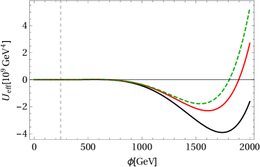
Deviations from the mean-field limit require relevant bosonic fluctuations. In the small coupling (i.e., small Higgs mass) regime, this can indeed occur in the full flow due to threshold effects of the following type: if a second minimum emerges seeded by a suitable bare potential, the curvature near the top of the barrier between the minima is negative, such that the bosonic threshold function is enhanced. This type of bosonic enhancement is only visible in a full potential flow. For a meaningful comparison between mean-field and full flow, we tune the bare potential such that the IR physics including the Higgs mass is kept fixed. For illustrative purposes, we choose a UV cutoff of only TeV, a Higgs mass of 25GeV and . The resulting potentials end up in the metastable regime as depicted in Fig. 10. The mean-field potential (dashed line) differs from the full solutions (solid lines) integrated down to an IR value of GeV. The full solutions correspond to defining the anomalous dimensions at the local Fermi minimum (black) or at the second global minimum (red). These curves differ as fields and couplings are renormalized differently within the two schemes, with the black curve corresponding to a renormalization choice better resolving the Fermi minimum and the red curve better suited for the second minimum. In other words, the axes for the different solid lines have a different meaning due to the different field rescaling during the flow. If the anomalous dimensions were artificially set to zero, mean-field and full potential results would still match rather well.
IV.5 Convexity of the effective potential
By definition of the effective action as a Legendre transform of the Schwinger functional, we expect the full effective action and particularly the effective potential to be convex functions of the field. This convexity property cannot be seen neither in the perturbative construction of the single-scale potential nor in the mean-field approximation. The Wetterich equation does have this convexity property in the limit for the bosonic potential, see e.g. Berges et al. (2002); Litim et al. (2006). However, at finite , the regulator term sources a non-convex contribution which vanishes in the limit .
For potentials with a single minimum, it is known that convexity of the running potential sets in rather late in RG time, i.e., convexity is driven by the very deep IR modes which are often no longer relevant for the IR observables. For instance in the examples above, we have stopped the flow at scales GeV, where the IR Fermi scale observables have already settled to their physical values. Still, for these values of , the approach to convexity has not fully set in yet. Whereas this demonstrates that convexity is not important for the static observables, it is an interesting question as to whether the approach to convexity can be important for estimates of the tunneling rate between two different minima. The relevance of this question becomes obvious from the fact that any tunneling barrier in a convex potential is (naively) exactly zero by construction.
In order to understand the onset of convexity in the present model, let us start with the simpler case with only one minimum at the Fermi scale. Here, convexity only affects the inner region of the potential with . Technically, convexity of the effective potential is generated by singularities in the bosonic propagators entering the threshold functions. In the present case, the bosonic threshold function corresponding to the regularized propagator is proportional to
| (26) |
exhibiting a singularity at , or for small or small . The flow avoids this singularity by renormalizing the negative curvature of the potential in the inner region with . This establishes convexity for .
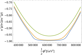
In comparison to purely bosonic models, fermionic fluctuations delay convexity since they enter the flow equation with an opposite sign, cf. the last term in Eq. (21). Thus, bosonic fluctuations have to exceed the fermionic fluctuations first. As convexity also introduces a non-analyticity at , its onset becomes numerically first visible in higher derivatives. Therefore, we consider the first derivative of the potential in the following. The balancing between bosons and fermions also implies that the onset of convexity becomes more pronounced if the boson coupling is enhanced relative to the fermion coupling . In terms of physical parameters, this implies that convexity should become more prominent for larger Higgs-to-top mass ratios. In Fig. 11, we plot for three different ratios . The flow has been stopped at a scale such that the potentials have the same distance from the singularity of the bosonic propagator . The faster approach to convexity then is directly visible in terms of the position of non-analyticity which we observe to move towards larger field amplitudes if increases. By contrast, if is small, the characteristic flat region of is hardly visible at this particular scale and would increase only towards even smaller scales.
It should be emphasized that convexity is a notoriously difficult problem for pseudo-spectral methods, since it introduces a non-analyticity which violates the assumptions on the function space for which exponential convergence can be proved. Hence, the numerics will unavoidably face a singularity problem in the very deep IR. For further adapted methods, see Bonanno and Lacagnina (2004); Peláez and Wschebor (2015).
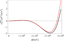
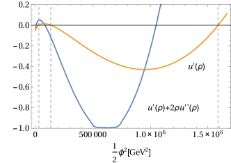
Let us now turn to the more interesting case of two minima which is numerically more challenging since the field-dependent “mass term” becomes negative, , not only for small fields but also for a second region at larger fields. As an illustrative example, we choose a similar flow as above. We plot this mass term in the region of both minima of the tunnel barrier, cf. Fig. 12 (left panel). For comparison we show as well. The dashed vertical lines indicate the position of both minima and the maximum in between. Convexity becomes first visible for larger fields at the minimum of the mass term which tends to after has dropped below the scale of the top quark, cf. Fig. 12 (right panel). For the current example, this minimum of the mass term is located in between the maximum and the outer minimum of the potential, but this relative position may vary depending on the scale and the precise choice of parameters. As the maximum of the potential is situated within the region where for larger fields, the flat region eventually extends beyond the maximum, significantly affecting the tunnel barrier for small scales . For small fields, the fermions still control the flow at GeV. However, for decreasing scale the bosonic fluctuations win out over the fermionic ones and convexity sets in as well, similar to Fig. 11. We emphasize that the approach to convexity appears to set in at different scales for large field amplitudes than for small ones.
In the present example, convexity affects the tunnel barrier at scales which are more than an order of magnitude smaller than the field amplitude of the barrier and the outer minimum. A calculation of the tunnel rate which is dominated by the latter scales hence is expected to be only weakly influenced by the approach to convexity. As a general rule, we conclude that the standard recipes for calculations of the tunnel rate Coleman (1977); Callan and Coleman (1977) remain unaffected as long as the fermion fluctuations dominate the renormalization of the potential. Whether or not this is the case at the relevant scales of interest will in general depend on the details of the scale-dependent potential and thus also on the details of the bare potential. As soon as the boson fluctuations become important, the approach to convexity has also be accounted for in estimates of the tunneling rate.
In the functional RG context, a proposal for this has been worked out for scalar models in Strumia et al. (1999). A formalism that can also systematically deal with further radiative effects in the resulting inhomogeneous instanton background on top of a radiatively generated potential has recently been developed with the help of a self-consistent functional scheme based on the 2PI effective action Garbrecht and Millington (2015a, b).
We would like to emphasize the necessity of a simultaneous consistent treatment of the renormalization flow of the potential together with the fluctuation contributions in a tunnel-rate calculation – even if the bare potential was known exactly. Of course, unknown higher dimensional operators then further add to the indeterminacy of the vacuum decay rate Branchina and Messina (2013); Branchina et al. (2014, 2015); Lalak et al. (2014); Eichhorn et al. (2015). For instance, the influence of gravity-induced higher dimensional operators has been studied in Loebbert and Plefka (2015); Bhattacharjee and Majumdar (2014); Haba et al. (2015); Abe et al. (2016).
IV.6 Quantum phase diagram of the Higgs-Yukawa model
Can the outer global minimum be used to define the electroweak vacuum? If the occurrence of metastability is rather generic in presence of higher-dimensional operators, could it be possible to fix physical parameters with respect to the global minimum as the Fermi scale? In order to address these questions, we now reconsider the model from a more general viewpoint.
So far, we have fixed the model with the help of the renormalization conditions (2) applied to the first or innermost minimum. Instead, let us now start from a fixed UV cutoff with some bare potential bounded from below and read off the IR phases from the effective potential at some IR scale where all modes have decoupled (apart from the approach to convexity). We are most interested in this quantum phase diagram as a function of the (super-)renormalizable operators and , as the electroweak precision data tells us that the standard model is sufficiently close to the Gaußian fixed point, where perturbation theory based on these operators works very well. In other words, higher-dimensional operators do not take a momentarily measurable influence on collider data.
In the language of critical phenomena, the standard model appears to be close to a second-order quantum phase transition that effectively allows to push the UV cutoff to large values (compared to collider scales). The natural candidate in the standard model is the electroweak (quantum) phase transition represented by the order-disorder phase transition of discrete chiral symmetry in our simple model. It is, in fact, straightforward to verify by means of perturbation theory, mean-field theory or the functional RG that this phase transition is of second order for type bare potentials in the stable regime. The “control parameter” for the quantum phase transition is the bare mass term .
In the following, we perform this investigation for the class of generalized bare potentials. For this, we fix as a representative of a higher-dimensional operator that induces absolute stability. We expect the following results to hold also for other polynomial operators that ensure absolute stability for large field amplitudes. For technical simplicity, we keep the Yukawa coupling fixed and also neglect the anomalous dimensions, as both do not induce qualitative differences. Still, we keep the full bosonic fluctuation contribution to the flow of the potential.
Choosing negative but with a small absolute value, the potential will still show only one minimum and the phase transition as a function of still is of second order as for the -class, cf. left-hand side of Fig. 13. Increasing the absolute value of a negative a bit, and starting with a large value of , the sufficiently negative may seed a local higher minimum at large field amplitudes. Nevertheless, the system is in the symmetric phase with the global minimum at (upper left part of Fig. 13). (On the left-hand side of this figure, we do not further distinguish between the existence or non-existence of a further local outer minima; potentials with a local outer minimum shown here only represent possible examples.)
Decreasing , we indeed observe a second-order phase transition to a broken phase driven by fermion fluctuations where the order parameter is switched on continuously, cf. white region in Fig. 13. A local higher minimum at larger field amplitudes may arise by decreasing or persists if it already existed. It is this second-order phase transition which can serve to define a “continuum limit” essentially establishing cutoff independence.
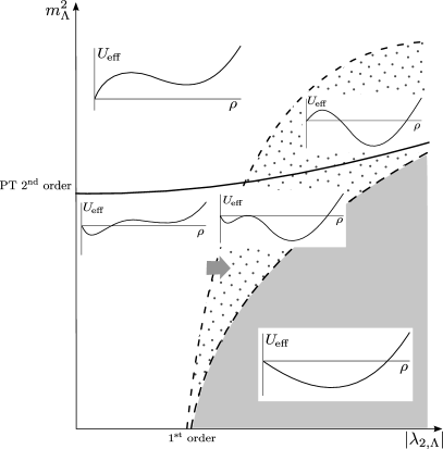
Decreasing further first leads to a lowering of the outer minimum such that the inner minimum becomes metastable (dotted region). The phase transition between the two cases is of first order (dashed lines). For even smaller mass parameters , the inner minimum vanishes discontinuously while the outer remains (gray-shaded region in Fig. 13). We also classify this discontinuous change of the system as a first-order transition, even though it would not correspond to a thermal phase transition: on both sides of the lower dashed line the system is dominated by the global minimum in the thermodynamic limit.
This analysis demonstrates that only the transition between the symmetric and the symmetry-broken phase, which is driven by fermion fluctuations, is of second order. Therefore, only this transition can be used to separate the cutoff scale from the IR physics in this model. This forces us to associate the Fermi scale with the innermost minimum driven by fermion-fluctuations. The outer one seeded by the bare action cannot be used for a definition of the Fermi scale as it is highly unlikely to match with the perturbative description of electroweak precision data. In our flows, this mismatch becomes visible in the practical difficulty to push the cutoff beyond TeV while satisfying all renormalization conditions with corresponding to the outer minimum.
For negative with an even larger absolute value (right-hand side of Fig. 13), the phase portraits are similar in the sense that only the transition driven by the fermionic fluctuations in the inner region of the potential is a second-order transition. The difference is that this transition occurs only after the outer minimum seeded by the bare action has become the global one. As a consequence, both the symmetric phase for larger as well as the fermion driven broken phase (inner minimum) are metastable (dotted region) on both sides of the transition. In this regime of bare potentials, the separation of IR physics from the UV scale hence goes along with a metastability.
We can also compare the phase portraits for fixed and use as control parameter. For instance, the transition marked by the gray thick arrow is a first-order broken-to-broken transition. This is likely to correspond to an equivalent transition first observed in lattice simulations of a similar chiral model Chu et al. (2015).
We emphasize that the phase portraits determined here correspond to quantum phase transitions with control parameters corresponding to parameters of the bare action. This is a priori unrelated to the nature of finite temperature phase transitions in the same model, even though a relation might be established dynamically because of a thermal decoupling of the fermions. For recent lattice studies, see Akerlund and de Forcrand (2015); Akerlund et al. (2015).
V Conclusions
We have investigated the renormalization flow of the effective scalar potential keeping the full dependence on all relevant scales: the field amplitude , an RG scale and the UV cutoff scale . This is necessary to overcome the limitations of conventional approximation schemes, relying on identifications such as , or implicit perturbative limits . The advantage of keeping the full scale dependence becomes obvious for the analysis of metastabilities.
Using a simple Higgs-Top-Yukawa model as an example, our analysis demonstrates that metastabilities are not primarily induced by fermion fluctuations, but have to be seeded by suitable structures in the bare potential. In particular, metastabilities cannot occur if a well-defined bare action is restricted to contain only renormalizable operators. Upon the inclusion of suitable higher-dimensional operators, metastabilities generically occur for small Higgs masses and large cutoffs – at least within the class of simple polynomial bare potentials studied in this work.
Whereas these latter conclusions are in part reminiscent to results obtained within perturbative estimates based on a single-scale effective potential (), it is worthwhile to note some decisive differences: our approach allows for addressing arbitrary bare potentials, defining the model purely in terms of its symmetry, field content and a minimal set of IR parameters. No assumption about the manifest absence of an infinity of irrelevant operators is made. While the occurrence of higher-dimensional operators is conventionally interpreted as particle physics beyond the standard model (e.g., induced by integrating out heavy particle multiplets), our approach allows to also associate such operators to any origin that can be parametrized in terms of any effective action, e.g., a coarse-grained continuum action in a spacetime arising from discrete building blocks.
In this work, we have studied global RG flows of the potential using pseudo-spectral methods. This facilitates to study the full RG evolution of competing minima, to analyze the quantum phase diagram of the model, and to quantify the approach to convexity. The latter is not accessible in perturbation theory or mean-field theory. The global flows also serve to confirm earlier results from local flows evaluated at the running Fermi minimum to a high accuracy, such as, for instance, the relaxation of the perturbative lower bound on the Higgs mass. On the other hand, the global flow also reveals the limitations of the local flow in metastable regimes as competing minima turn out to be beyond the radius of convergence of local flows. Further, the global flows also demonstrate the usefulness of the mean-field approximation in the small-Higgs-mass regime.
Finally, we emphasize that a full determination of consistency bounds for the IR observables of the standard model as a function of the cutoff as the scale of maximum UV extension has not yet been completed. For this, the mapping of a wide range of bare actions to the IR observables would have to be computed with the RG, technically corresponding to an extremization problem in an infinite-dimensional space. The capability of handling global flows and extending the current studies to nonpolynomial interactions will be a necessary prerequisite for this.
Acknowledgments
We thank Björn Garbrecht, Tobias Hellwig, Tina K. Herbst, Benjamin Knorr, Stefan Lippoldt, Peter Millington, Michael M. Scherer, Matthias Warschinke, and Luca Zambelli for valuable discussions. We acknowledge support by the DFG under Grants No. GRK1523/2 and No. Gi328/7-1.
References
- Aad et al. (2012) G. Aad et al. (ATLAS), Phys. Lett. B716, 1 (2012), arXiv:1207.7214 [hep-ex] .
- Chatrchyan et al. (2012) S. Chatrchyan et al. (CMS), Phys. Lett. B716, 30 (2012), arXiv:1207.7235 [hep-ex] .
- Maiani et al. (1978) L. Maiani, G. Parisi, and R. Petronzio, Nucl. Phys. B136, 115 (1978).
- Krasnikov (1978) N. V. Krasnikov, Yad. Fiz. 28, 549 (1978).
- Lindner (1986) M. Lindner, Z. Phys. C31, 295 (1986).
- Wetterich (1987) C. Wetterich, in Search for Scalar Particles: Experimental and Theoretical Aspects Trieste, Italy, July 23-24, 1987 (1987).
- Altarelli and Isidori (1994) G. Altarelli and G. Isidori, Phys. Lett. B337, 141 (1994).
- Schrempp and Wimmer (1996) B. Schrempp and M. Wimmer, Prog. Part. Nucl. Phys. 37, 1 (1996), arXiv:hep-ph/9606386 [hep-ph] .
- Hambye and Riesselmann (1997) T. Hambye and K. Riesselmann, Phys. Rev. D55, 7255 (1997), arXiv:hep-ph/9610272 [hep-ph] .
- Wetterich (1981) C. Wetterich, Phys. Lett. B104, 269 (1981).
- Bezrukov and Shaposhnikov (2015) F. Bezrukov and M. Shaposhnikov, J. Exp. Theor. Phys. 120, 335 (2015), arXiv:1411.1923 [hep-ph] .
- Krive and Linde (1976) I. V. Krive and A. D. Linde, Nucl. Phys. B117, 265 (1976).
- Hung (1979) P. Q. Hung, Phys. Rev. Lett. 42, 873 (1979).
- Linde (1980) A. D. Linde, Phys. Lett. B92, 119 (1980).
- Cabibbo et al. (1979) N. Cabibbo, L. Maiani, G. Parisi, and R. Petronzio, Nucl. Phys. B158, 295 (1979).
- Politzer and Wolfram (1979) H. D. Politzer and S. Wolfram, Phys. Lett. B82, 242 (1979), [Erratum: Phys. Lett.83B,421(1979)].
- Kuti et al. (1988) J. Kuti, L. Lin, and Y. Shen, Phys. Rev. Lett. 61, 678 (1988).
- Sher (1989) M. Sher, Phys. Rept. 179, 273 (1989).
- Hasenfratz et al. (1987) A. Hasenfratz, K. Jansen, C. B. Lang, T. Neuhaus, and H. Yoneyama, Phys. Lett. B199, 531 (1987).
- Luscher and Weisz (1989) M. Luscher and P. Weisz, Nucl. Phys. B318, 705 (1989).
- Lindner et al. (1989) M. Lindner, M. Sher, and H. W. Zaglauer, Phys. Lett. B228, 139 (1989).
- Ford et al. (1993) C. Ford, D. R. T. Jones, P. W. Stephenson, and M. B. Einhorn, Nucl. Phys. B395, 17 (1993), arXiv:hep-lat/9210033 [hep-lat] .
- Heller et al. (1993) U. M. Heller, M. Klomfass, H. Neuberger, and P. M. Vranas, Nucl. Phys. B405, 555 (1993), arXiv:hep-ph/9303215 [hep-ph] .
- Arnold (1989) P. B. Arnold, Phys. Rev. D40, 613 (1989).
- Sher (1993) M. Sher, Phys. Lett. B317, 159 (1993), [Addendum: Phys. Lett.B331,448(1994)], arXiv:hep-ph/9307342 [hep-ph] .
- Casas et al. (1995) J. A. Casas, J. R. Espinosa, and M. Quiros, Phys. Lett. B342, 171 (1995), arXiv:hep-ph/9409458 [hep-ph] .
- Espinosa and Quiros (1995) J. R. Espinosa and M. Quiros, Phys. Lett. B353, 257 (1995), arXiv:hep-ph/9504241 [hep-ph] .
- Bergerhoff et al. (1999) B. Bergerhoff, M. Lindner, and M. Weiser, Phys. Lett. B469, 61 (1999), arXiv:hep-ph/9909261 [hep-ph] .
- Isidori et al. (2001) G. Isidori, G. Ridolfi, and A. Strumia, Nucl. Phys. B609, 387 (2001), arXiv:hep-ph/0104016 [hep-ph] .
- Ellis et al. (2009) J. Ellis, J. R. Espinosa, G. F. Giudice, A. Hoecker, and A. Riotto, Phys. Lett. B679, 369 (2009), arXiv:0906.0954 [hep-ph] .
- Holthausen et al. (2012) M. Holthausen, K. S. Lim, and M. Lindner, JHEP 02, 037 (2012), arXiv:1112.2415 [hep-ph] .
- Elias-Miro et al. (2012) J. Elias-Miro, J. R. Espinosa, G. F. Giudice, G. Isidori, A. Riotto, and A. Strumia, Phys. Lett. B709, 222 (2012), arXiv:1112.3022 [hep-ph] .
- Degrassi et al. (2012) G. Degrassi, S. Di Vita, J. Elias-Miro, J. R. Espinosa, G. F. Giudice, G. Isidori, and A. Strumia, JHEP 08, 098 (2012), arXiv:1205.6497 [hep-ph] .
- Alekhin et al. (2012) S. Alekhin, A. Djouadi, and S. Moch, Phys. Lett. B716, 214 (2012), arXiv:1207.0980 [hep-ph] .
- Masina (2013) I. Masina, Phys. Rev. D87, 053001 (2013), arXiv:1209.0393 [hep-ph] .
- Buttazzo et al. (2013) D. Buttazzo, G. Degrassi, P. P. Giardino, G. F. Giudice, F. Sala, A. Salvio, and A. Strumia, JHEP 12, 089 (2013), arXiv:1307.3536 [hep-ph] .
- Gabrielli et al. (2014) E. Gabrielli, M. Heikinheimo, K. Kannike, A. Racioppi, M. Raidal, and C. Spethmann, Phys. Rev. D89, 015017 (2014), arXiv:1309.6632 [hep-ph] .
- Bednyakov et al. (2015) A. V. Bednyakov, B. A. Kniehl, A. F. Pikelner, and O. L. Veretin, Phys. Rev. Lett. 115, 201802 (2015), arXiv:1507.08833 [hep-ph] .
- Gies et al. (2014) H. Gies, C. Gneiting, and R. Sondenheimer, Phys. Rev. D89, 045012 (2014), arXiv:1308.5075 [hep-ph] .
- Gies and Sondenheimer (2015) H. Gies and R. Sondenheimer, Eur. Phys. J. C75, 68 (2015), arXiv:1407.8124 [hep-ph] .
- Eichhorn et al. (2015) A. Eichhorn, H. Gies, J. Jaeckel, T. Plehn, M. M. Scherer, and R. Sondenheimer, JHEP 04, 022 (2015), arXiv:1501.02812 [hep-ph] .
- Hegde et al. (2014) P. Hegde, K. Jansen, C. J. D. Lin, and A. Nagy, Proceedings, 31st International Symposium on Lattice Field Theory (Lattice 2013), PoS LATTICE2013, 058 (2014), arXiv:1310.6260 [hep-lat] .
- Chu et al. (2015) D. Y. J. Chu, K. Jansen, B. Knippschild, C. J. D. Lin, and A. Nagy, Phys. Lett. B744, 146 (2015), arXiv:1501.05440 [hep-lat] .
- Chu et al. (2014) D. Y. J. Chu, K. Jansen, B. Knippschild, C. J. D. Lin, K.-I. Nagai, and A. Nagy, Proceedings, 32nd International Symposium on Lattice Field Theory (Lattice 2014), PoS LATTICE2014, 278 (2014), arXiv:1501.00306 [hep-lat] .
- Akerlund and de Forcrand (2015) O. Akerlund and P. de Forcrand, (2015), arXiv:1508.07959 [hep-lat] .
- Eichhorn and Scherer (2014) A. Eichhorn and M. M. Scherer, Phys. Rev. D90, 025023 (2014), arXiv:1404.5962 [hep-ph] .
- Jakovac et al. (2015a) A. Jakovac, I. Kaposvari, and A. Patkos, (2015a), arXiv:1508.06774 [hep-th] .
- Jakovac et al. (2015b) A. Jakovac, I. Kaposvari, and A. Patkos, (2015b), arXiv:1510.05782 [hep-th] .
- Datta et al. (1996) A. Datta, B. L. Young, and X. Zhang, Phys. Lett. B385, 225 (1996), arXiv:hep-ph/9604312 [hep-ph] .
- Barbieri and Strumia (1999) R. Barbieri and A. Strumia, Phys. Lett. B462, 144 (1999), arXiv:hep-ph/9905281 [hep-ph] .
- Grzadkowski and Wudka (2002) B. Grzadkowski and J. Wudka, Phys. Rev. Lett. 88, 041802 (2002), arXiv:hep-ph/0106233 [hep-ph] .
- Burgess et al. (2002) C. P. Burgess, V. Di Clemente, and J. R. Espinosa, JHEP 01, 041 (2002), arXiv:hep-ph/0201160 [hep-ph] .
- Barger et al. (2003) V. Barger, T. Han, P. Langacker, B. McElrath, and P. Zerwas, Phys. Rev. D67, 115001 (2003), arXiv:hep-ph/0301097 [hep-ph] .
- Blum et al. (2015) K. Blum, R. T. D’Agnolo, and J. Fan, JHEP 03, 166 (2015), arXiv:1502.01045 [hep-ph] .
- Borchardt and Knorr (2015) J. Borchardt and B. Knorr, Phys. Rev. D91, 105011 (2015), arXiv:1502.07511 [hep-th] .
- (56) J. Borchardt and B. Knorr, “Solving functional flow equations with pseudo-spectral methods ,” In preparation.
- Holland and Kuti (2004) K. Holland and J. Kuti, Lattice hadron physics. Proceedings, 2nd Topical Workshop, LHP 2003, Cairns, Australia, July 22-30, 2003, Nucl. Phys. Proc. Suppl. 129, 765 (2004), [,765(2003)], arXiv:hep-lat/0308020 [hep-lat] .
- Holland (2005) K. Holland, Lattice field theory. Proceedings, 22nd International Symposium, Lattice 2004, Batavia, USA, June 21-26, 2004, Nucl. Phys. Proc. Suppl. 140, 155 (2005), [,155(2004)], arXiv:hep-lat/0409112 [hep-lat] .
- Branchina and Faivre (2005) V. Branchina and H. Faivre, Phys. Rev. D72, 065017 (2005), arXiv:hep-th/0503188 [hep-th] .
- Krajewski and Lalak (2015) T. Krajewski and Z. Lalak, Phys. Rev. D92, 075009 (2015), arXiv:1411.6435 [hep-ph] .
- Coleman and Weinberg (1973) S. R. Coleman and E. J. Weinberg, Phys. Rev. D7, 1888 (1973).
- Andreassen et al. (2014) A. Andreassen, W. Frost, and M. D. Schwartz, Phys. Rev. Lett. 113, 241801 (2014), arXiv:1408.0292 [hep-ph] .
- Andreassen et al. (2015) A. Andreassen, W. Frost, and M. D. Schwartz, Phys. Rev. D91, 016009 (2015), arXiv:1408.0287 [hep-ph] .
- Litim (2000) D. F. Litim, Phys. Lett. B486, 92 (2000), arXiv:hep-th/0005245 [hep-th] .
- Litim (2001) D. F. Litim, Phys. Rev. D64, 105007 (2001), arXiv:hep-th/0103195 [hep-th] .
- Fodor et al. (2007) Z. Fodor, K. Holland, J. Kuti, D. Nogradi, and C. Schroeder, Proceedings, 25th International Symposium on Lattice field theory (Lattice 2007), PoS LAT2007, 056 (2007), arXiv:0710.3151 [hep-lat] .
- Gerhold and Jansen (2007a) P. Gerhold and K. Jansen, JHEP 09, 041 (2007a), arXiv:0705.2539 [hep-lat] .
- Gerhold and Jansen (2007b) P. Gerhold and K. Jansen, JHEP 10, 001 (2007b), arXiv:0707.3849 [hep-lat] .
- Gerhold and Jansen (2009) P. Gerhold and K. Jansen, JHEP 07, 025 (2009), arXiv:0902.4135 [hep-lat] .
- Gerhold et al. (2011) P. Gerhold, K. Jansen, and J. Kallarackal, JHEP 01, 143 (2011), arXiv:1011.1648 [hep-lat] .
- Bulava et al. (2013a) J. Bulava, P. Gerhold, K. Jansen, J. Kallarackal, B. Knippschild, C. J. D. Lin, K.-I. Nagai, A. Nagy, and K. Ogawa, Adv. High Energy Phys. 2013, 875612 (2013a), arXiv:1210.1798 [hep-lat] .
- Bulava et al. (2013b) J. Bulava, K. Jansen, and A. Nagy, Phys. Lett. B723, 95 (2013b), arXiv:1301.3416 [hep-lat] .
- Djouadi and Lenz (2012) A. Djouadi and A. Lenz, Phys. Lett. B715, 310 (2012), arXiv:1204.1252 [hep-ph] .
- Hebecker et al. (2013) A. Hebecker, A. K. Knochel, and T. Weigand, Nucl. Phys. B874, 1 (2013), arXiv:1304.2767 [hep-th] .
- Wetterich (1993) C. Wetterich, Phys. Lett. B301, 90 (1993).
- Berges et al. (2002) J. Berges, N. Tetradis, and C. Wetterich, Phys. Rept. 363, 223 (2002), arXiv:hep-ph/0005122 [hep-ph] .
- Pawlowski (2007) J. M. Pawlowski, Annals Phys. 322, 2831 (2007), arXiv:hep-th/0512261 [hep-th] .
- Gies (2012) H. Gies, ECT* School on Renormalization Group and Effective Field Theory Approaches to Many-Body Systems Trento, Italy, February 27-March 10, 2006, Lect. Notes Phys. 852, 287 (2012), arXiv:hep-ph/0611146 [hep-ph] .
- Delamotte (2012) B. Delamotte, Lect. Notes Phys. 852, 49 (2012), arXiv:cond-mat/0702365 [cond-mat.stat-mech] .
- Braun (2012) J. Braun, J. Phys. G39, 033001 (2012), arXiv:1108.4449 [hep-ph] .
- Gies and Scherer (2010) H. Gies and M. M. Scherer, Eur. Phys. J. C66, 387 (2010), arXiv:0901.2459 [hep-th] .
- Vacca and Zambelli (2015) G. P. Vacca and L. Zambelli, Phys. Rev. D91, 125003 (2015), arXiv:1503.09136 [hep-th] .
- Bohr et al. (2001) O. Bohr, B. J. Schaefer, and J. Wambach, Int. J. Mod. Phys. A16, 3823 (2001), arXiv:hep-ph/0007098 [hep-ph] .
- Herbst et al. (2013) T. K. Herbst, J. M. Pawlowski, and B.-J. Schaefer, Phys. Rev. D88, 014007 (2013), arXiv:1302.1426 [hep-ph] .
- Adams et al. (1995) J. A. Adams, J. Berges, S. Bornholdt, F. Freire, N. Tetradis, and C. Wetterich, Mod. Phys. Lett. A10, 2367 (1995), arXiv:hep-th/9507093 [hep-th] .
- Hofling et al. (2002) F. Hofling, C. Nowak, and C. Wetterich, Phys. Rev. B66, 205111 (2002), arXiv:cond-mat/0203588 [cond-mat] .
- Bonanno and Zappala (2001) A. Bonanno and D. Zappala, Phys. Lett. B504, 181 (2001), arXiv:hep-th/0010095 [hep-th] .
- Boettcher et al. (2015) I. Boettcher, J. Braun, T. K. Herbst, J. M. Pawlowski, D. Roscher, and C. Wetterich, Phys. Rev. A91, 013610 (2015), arXiv:1409.5070 [cond-mat.quant-gas] .
- O’Raifeartaigh et al. (1986) L. O’Raifeartaigh, A. Wipf, and H. Yoneyama, Nucl. Phys. B271, 653 (1986).
- Litim et al. (2006) D. F. Litim, J. M. Pawlowski, and L. Vergara, (2006), arXiv:hep-th/0602140 [hep-th] .
- Boyd (2000) J. P. Boyd, Chebyshev and Fourier Spectral Methods, 2nd ed. (Dover Publications, 2000).
- Robson and Prytz (1993) R. Robson and A. Prytz, Australian Journal of Physics 46 (1993).
- Fischer and Gies (2004) C. S. Fischer and H. Gies, JHEP 10, 048 (2004), arXiv:hep-ph/0408089 [hep-ph] .
- (94) C. Gneiting, “Diploma thesis,” Heidelberg 2005.
- Bonanno and Lacagnina (2004) A. Bonanno and G. Lacagnina, Nucl. Phys. B693, 36 (2004), arXiv:hep-th/0403176 [hep-th] .
- Peláez and Wschebor (2015) M. Peláez and N. Wschebor, (2015), arXiv:1510.05709 [cond-mat.stat-mech] .
- Coleman (1977) S. R. Coleman, Phys. Rev. D15, 2929 (1977), [Erratum: Phys. Rev.D16,1248(1977)].
- Callan and Coleman (1977) C. G. Callan, Jr. and S. R. Coleman, Phys. Rev. D16, 1762 (1977).
- Strumia et al. (1999) A. Strumia, N. Tetradis, and C. Wetterich, Phys. Lett. B467, 279 (1999), arXiv:hep-ph/9808263 [hep-ph] .
- Garbrecht and Millington (2015a) B. Garbrecht and P. Millington, Phys. Rev. D91, 105021 (2015a), arXiv:1501.07466 [hep-th] .
- Garbrecht and Millington (2015b) B. Garbrecht and P. Millington, Phys. Rev. D92, 125022 (2015b), arXiv:1509.08480 [hep-ph] .
- Branchina and Messina (2013) V. Branchina and E. Messina, Phys. Rev. Lett. 111, 241801 (2013), arXiv:1307.5193 [hep-ph] .
- Branchina et al. (2014) V. Branchina, E. Messina, and A. Platania, JHEP 09, 182 (2014), arXiv:1407.4112 [hep-ph] .
- Branchina et al. (2015) V. Branchina, E. Messina, and M. Sher, Phys. Rev. D91, 013003 (2015), arXiv:1408.5302 [hep-ph] .
- Lalak et al. (2014) Z. Lalak, M. Lewicki, and P. Olszewski, JHEP 05, 119 (2014), arXiv:1402.3826 [hep-ph] .
- Loebbert and Plefka (2015) F. Loebbert and J. Plefka, (2015), arXiv:1502.03093 [hep-ph] .
- Bhattacharjee and Majumdar (2014) S. Bhattacharjee and P. Majumdar, Nucl. Phys. B885, 481 (2014), arXiv:1210.0497 [hep-th] .
- Haba et al. (2015) N. Haba, K. Kaneta, R. Takahashi, and Y. Yamaguchi, Phys. Rev. D91, 016004 (2015), arXiv:1408.5548 [hep-ph] .
- Abe et al. (2016) Y. Abe, M. Horikoshi, and T. Inami, (2016), arXiv:1602.03792 [hep-ph] .
- Akerlund et al. (2015) O. Akerlund, P. de Forcrand, and J. Steinbauer, in Proceedings, 33rd International Symposium on Lattice Field Theory (Lattice 2015) (2015) arXiv:1511.03867 [hep-lat] .