Numerical simulations of the jetted tidal disruption event Swift J1644+57

Abstract

In this work we focus on the technical details of the numerical simulations of the non-thermal transient Swift J1644+57, whose emission is probably produced by a two-component jet powered by a tidal disruption event. In this context we provide details of the coupling between the relativistic hydrodynamic simulations and the radiative transfer code. First, we consider the technical demands of one-dimensional simulations of a fast relativistic jet, and show to what extent (for the same physical parameters of the model) do the computed light curves depend on the numerical parameters of the different codes employed. In the second part we explain the difficulties of computing light curves from axisymmetric two dimensonal simulations and discuss a procedure that yields an acceptable tradeoff between the computational cost and the quality of the results.

1 Introduction

Tidal disruption events (TDE) of stars by massive black holes [1, 2, 3] provide one of the ways to detect an inactive massive black hole in the center of a galaxy. Stars whose orbit brings them too close to a black hole can be disrupted and a large fraction of their mass can be accreted. This sudden accretion event is expected to produce a luminous UV and X-ray TDE flare [4, 5]. It has recently been argued that TDEs can also produce jets [6, 7, 8]. These jets are expected to be detectable due to their non-thermal emission, and in radio they are likely to appear as transients that peak on the timescales of about a year [6, 9] after the tidal disruption.

Swift J1644+57 (SwJ1644 in the rest of the article) is a non-thermal transient detected on March 28th. 2011 [10, 11, 12]. It is thought to be prototype of a jetted TDE (jTDE). Its radio emission [13, 14, 15] is long-lived and complex. One of the first attempts to explain the radio emission of Swift J1644+57 using one-dimensional models and relativistic hydrodynamic simulations[16] assumed that the emission is coming from the shocks that form when the jet interacts with the circumnuclear medium (CNM). This model is more analogous to a GRB afterglow than to an AGN. While the model was successful in explaining the first few weeks of SwJ1644 radio emission, it turns out that the long-term emission is not easily accounted for by a radio afterglow from a single ultrarelativistic, narrow jet. The reason for this is that the source rebrightened after $\mathbin{\lower 3.0pt\hbox{$\hbox to0.0pt{\raise 5.0pt\hbox{$\char 62\relax$}\hss}\mathchar 29208\relax$}}150$ days, the time at which the afterglow model predicted a steady decline[14, Figure 1]. The late time rebrightening implies that additional energy is injected in the external shock months after the burst[14]. This may happen if, for instance, the jTDE is accompanied by a powerful mildly relativistic component[18].

In this contribution we focus on the numerical and technical aspects of jTDE modeling. In Section 2 we describe the numerical codes used in the calculations and how they depend on each other. The Section 3 gives an overview of computational requirements and their consequences on the kind of models that we were able to produce. The discussion and summary is given in the Section 4.

2 Numerical codes

SwJ1644 is a distant object (its redsfhit is $z=0.354$ [10]), and is thus too small to be resolved in great detail. Thus, the only direct observations that we have are the total fluxes for different times and frequencies (i.e., multiwavelength light curves). Nevertheless, when simulating this source we need to construct a detailed, resolved model of the SwJ1644 jet, simulate its dynamics, compute its resolved emission, and only in the final stage integrate the resolved emission to compute the total flux to be compared to observations. In order to achieve this we use two numerical codes so that the output of the first code (MRGENESIS) is used as an input to the second one (SPEV). The former simulates the jet dynamics, while the latter computes its emission.

2.1 Relativistic hydrodynamics simulations

MRGENESIS is a code developed to solve the equations of relativistic numerical (magneto) hydrodynamics in the laboratory frame (i.e., a frame at rest with respect to the distant source). The code is massively parallelized using MPI and OpenMP librararies, and uses the parallel HDF5 library for file input and output. We employ a method of lines for our simulations in which the spatial reconstruction is a based on the third order PPM reconstruction routines[22], and the time update is performed by means of a third order TVD Runge-Kutta scheme[23]. Numerical fluxes are evaluated with the Marquina flux formula[24]. We simulate SwJ1644 in two dimensions assuming axisymmetry and discretize the computational domain using spherical coordinates. The black hole is assumed to be located at the origin and the TDE occurs at scales that are much smaller than the ones we consider in our work (we simulate neither the TDE nor the jet launching). We set the beginning of the numerical grid at $\sim 10^{16}$ cm. The jet is injected through the inner boundary in an angular interval $[0,\theta_{j}]$, assuming a constant Lorentz factor $\Gamma_{j}$, and a luminosity whose time dependence is $L_{j}(t)=L_{j,0}\max[1,(t/t_{0})]^{-5/3}$. $t_{0}$ is the time during which the jet luminosity is constant, and the peak lumiosity $L_{j,0}$ is computed from the total jTDE energy $E_{\rm ISO}$ through $L_{j,0}=2E_{\rm ISO}/(5t_{0})$. The jet interacts with a CNM that is assumed to be at rest with a density profile $\rho_{\rm cnm}=n_{18}m_{p}(r/10^{18}{\rm cm})^{-k}$, where $m_{p}$ is the proton mass, $n_{18}$ is the particle number density at $10^{18}$ cm and $k$ is the power-law index of the density profile. We assume that initially both the jet and the external medium are cold. During the simulation we periodically store the snapshots of the computational grid in order to obtain a sufficient coverage of the jet-CNM interaction to be able to compute the resulting emission with sufficient precision (see Section 3).

2.2 Radiative transfer

Once the relativistic hydrodynamics simulation has finished, the snapshots it produced are used by the code SPEV to compute the emission. The spatial distribution of the hydrodynamics variables needs to be stored with sufficient frequency because of the space-time transformations that need to be performed to compute the observable radiation in the (distant) observer frame. SPEV[25] is designed to process an arbitrary number of pre-computed sets of hydrodynamic states of the fluid (i.e., density, pressure, positions, velocities, magnetic field) and to compute the resulting non-thermal emission. The procedure can be summarized as follows:

1. Injection: SPEV uses a set of Lagrangian particles (LPs) as a representation of the emitting volumes. Each LP has a defined position, shape and velocity. Attached to it there is a representation of the non-thermal electron (NTE) energy distribution. In SPEV, new LPs are created each time a snapshot is processed. The position of the shock fronts that form as a consequence of the jet-CNM interaction is detected, and LPs are injected into the shocked fluid immediately behind the front. Since the actual process of particle acceleration occurs on temporal and spatial scales far below the ones we are able to simulate (see e.g., [26] for a recent review), we use a phenomenological model to link the fluid state with NTE distribution. The model we use is a standard one [27]: the energy contained in the NTEs and in the stochastic magnetic field are assumed to be fractions $\epsilon_{e}$ and $\epsilon_{B}$ of the shocked fluid thermal energy. The injection spectrum is assumed to be a power-law in energy $n(\gamma)\propto\gamma^{-p}$, where $p$ is the power-law index and $\gamma$ is the NTE Lorentz factor. We determine the normalization and energy cutoffs of the distribution using a numerical procedure described in detail in Sections 3.2 and 3.3 of [28].

2. Transport, evolution and emission: As it processes the snapshots, SPEV transports the injected LPs, assuming that after they have been injected they move with the fluid. An exception are the newly injected LPs: between the snapshot in which the particle is injected and the subsequent one the two edges parallel to the shock front are assumed to move with different velocities (one with the velocity of the shocked fluid and the other one with the faster velocity of the shock front). This ensures that new LPs correctly represent the increase in the volume due to newly shocked fluid, regardless of the numerical resolution or the frequency with which snapshots are stored. Simultaneously, the NTE energy losses due to synchrotron radiation, as well as the energy gains(losses) due to adiabatic compression(expansion) are taken into account:

   $${\frac{\mathrm{d}\gamma}{\mathrm{d}t}}=\displaystyle{\frac{1}{3}}\displaystyle{\frac{\mathrm{d}\ln\rho}{\mathrm{d}t}}\gamma-\displaystyle{\frac{4}{3}}\displaystyle{\frac{c\sigma_{T}}{m_{e}c^{2}}}\left(u_{B}+u_{\rm rad}\right)\gamma^{2}\,$$ (1)

   where $t$, $\rho$, $u_{B}$ and $u_{\rm rad}$ are the time, fluid density, magnetic field energy density and external radiation field energy density (all measured in the LP frame). Section 3.2 of [25] describes an efficient numerical algorithm for solving Eq. 1 for each NTE distribution in each LP. At the same time that the particles are evolved, their non-thermal emission is computed (see Section 4 of [25] for a description of an efficient numerical algorithm for computing synchrotron emission and absorption coefficients, and Section A.2.1 of the same paper for a description of the way particles in two-dimensional axisymmetric models can be used to represent three-dimensional emitting volumes). The coefficients computed in this step are stored in a global array that is used in the final step.

3. Solving the radiative transfer equation: After all the snapshots have been processed and the emission from all LPs has been computed for all times, the time- and frequency-dependent emission can be computed. We assume that there is a virtual screen (“virtual detector”, VD) located in front of the source, and the goal is to compute the intensity in each of the virtual pixels of the VD. This is done by solving the radiative transfer equation

   $${\frac{\mathrm{d}I_{\nu}}{\mathrm{d}s}}=j_{\nu}-\alpha_{\nu}I_{\nu},,$$ (2)

   where $I_{\nu}$, $j_{\nu}$ and $\alpha_{\nu}$ are the specific intensity, emissivity and absorption coefficient. $s$ is the distance along the line of sight from the jet to a particular pixel and it relates the simulation time $t$ to the time of observation $T$ by $t=T+(D-s)/c$, where $D$ is the distance from the VD to the source. In other words, for a given $T$ and $t$, $s$ is the distance of a LP from which radiation is observed at time $T$ if that LP is emitting at a time $t$. We note that Eq. 2 needs to be solved in such a way that $s$ is monotonously increasing from the jet towards the VD. Therefore, after all the snapshots have been processed, the emission and absorption coefficients need to be sorted according to their $s$ and then Eq. 2 is solved for each pixel.

In practice the positions of LPs in steps (i) and (ii) are stored in a set of (large) intermediate files (“preprocessor” files). A postprocessor executes the radiation part of step (ii) by reading the preprocessor files and storing the coefficients in memory. After all preprocessor files have been postprocessed, the step (iii) is executed. Both preprocessor and postprocessor parts of SPEV are paralellized using OpenMP. The postprocessor, in particular, needs to be run on a machine with enough shared memory because all information produced in step 2 needs to be held in memory for the step 3 to correctly compute the intensities.

3 Simulations of Swift J1644+57 jet

As mentioned in Section 2.1, we model SwJ1644 jet in two-dimensions. However, as will be explained in this Section, the total cost in terms of computing time, disk storage and working memory of each two-dimensional simulation is high. Therefore, we first perform a number of much less costly tests using a one-dimensional approximation to two-dimensional models. The goal of those tests is to determine the values of a number of the parameters of the numerical simulation for which the results are satisfactory. Afterward, the two-dimensional simulations are performed using the values determined in one-dimensional tests.

3.1 One-dimensional tests

Using MRGENESIS we simulate one-dimensional spherically symmetric jets. For the purpose of computing their emission with SPEV we assume that their opening angles are $\theta_{j}$. We fix all the physical parameters of the jet ($E_{\rm ISO}=4\times 10^{54}$ erg, $\Gamma_{j}=10$, $\theta_{j}=0.1$ rad, $t_{0}=5\times 10^{5}$ s) and of the external medium ($n_{18}=60$ cm^-3, $k=1.5$). This corresponds to the inner relativistic component of the two-component jet in [18]. The numerical parameters that will be varied are:

• $\Delta T_{\rm snap}$: time interval between snapshots (MRGENESIS)

• $\Delta r$: radial resolution (MRGENESIS)

• $\Delta\theta$: angular resolution (MRGENESIS)

• $N_{b}$: number of NTE energy distribution bins (SPEV)

• $n_{x}$: resolution of the virtual detector (SPEV)

We choose as a default set of parameters $\Delta T_{\rm snap}=8.3\times 10^{4}$ s, $\Delta r=5\times 10^{13}$ cm, $\Delta\theta=2\times 10^{-3}$ rad, $N_{b}=32$, $n_{x}=1000$. We follow the jet evolution until $\sim 6.7\times 10^{8}$ seconds. During the first $1.3\times 10^{8}$ seconds the snapshots are output every $\Delta T_{\rm snap}$, and afterward the time interval increases by a factor $1.002$ after every snapshot is output.

Fig. 1 shows the light curves for the default model evaluated at 1.4 GHz (red line) and the consequence of variations in the resolution of the hydrodynamic models, i.e., as a result of changing $\Delta r$. As can be seen, relatively small differences of the order of a percent are visible at early times and after the light curve maximum. The top right panel in Fig. 1 shows the result of changing angular resolution. Here the differences are somewhat larger, especially when comparing the lowest and highest resolution ($\sim 4$% at peak). The middle left panel in Fig. 1 shows how the results depend on the number of bins in which NTE energy distribution of each LP is discretized. We see that the convergence is only achieved for $N_{b}\mathbin{\lower 3.0pt\hbox{$\hbox to0.0pt{\raise 5.0pt\hbox{$\char 62\relax$}\hss}\mathchar 29208\relax$}}32$. In the middle right panel we can see that the oscillations at early times are due to poor VD resolution. The angular size of the jet is very small at those times and it is only properly resolved for $n_{x}\sim 10^{4}$ for a linear pixel distribution (covering the interval [$0$, $5\times 10^{18}$ cm]), and $n_{x}\sim 10^{3}$ for a logarithmic one (covering the interval [$10^{12}$ cm, $5\times 10^{18}$ cm]). In the next section we will explain how we solved the problem of noise for 2D simulation light curves, especially the off-axis ones where it is not feasible to distribute the VD pixels logarithmically. Finally, the bottom left panel shows the (weak) dependence on $\Delta T_{\rm snap}$.

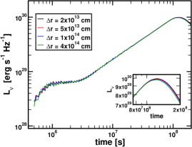
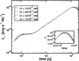
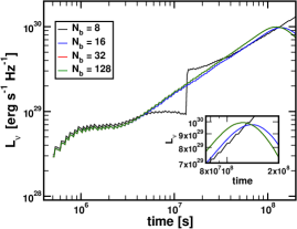
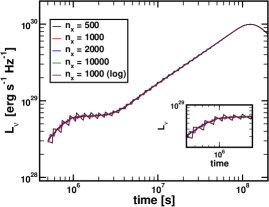
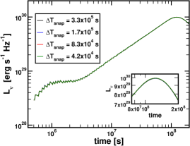
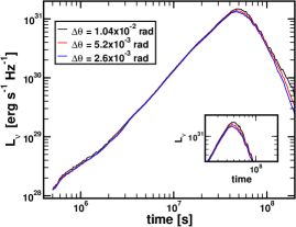
Figure 1: $1.4$ GHz radio light curves of one-dimensional tests (Section 3.1). The default model is shown in red. The insets show the zoom-in around the light curve maximum. Top left panel: Variations in $\Delta r$. Top right panel: Variations in $\Delta\theta$. Middle left panel: Variations in the number of bins $N_{b}$. Note that $N_{b}=32$ and $N_{b}=128$ curves overlap. Middle right panel: Variations in the number of VD pixels. Note that the curves for $n_{x}=10^{4}$ and $n_{x}=10^{3}$ with a logarithmic distribution of pixels overlap. Bottom left panel: Variations in $\Delta T_{\rm snap}$. Bottom right panel: Emission from two dimensional two-component jet for different effective angular resolutions (see Section 3.2).

3.2 Two-dimensional simulations

In the previous section we showed how the light curves change as the five principal numerical parameters are changed. Most importantly for the 2D simulations, with the previous tests we have already obtained a very good proxy for the largest values of $\Delta r$ and $\Delta\theta$ we can use in order to reduce the computational cost without compromising the accuracy of the results. In the final simulations showed in [18] we used $\Delta r=4\times 10^{14}$ cm and $\Delta\theta\simeq 2.6\times 10^{-3}$ rad. In this section we discuss the technical challenges of computing the emission even from these relatively low-resolution hydrodynamic simulations.

The complete two-dimensional evolution is stored in $2412$ snapshots. It was fortunate that HDF5 format permits data compression so that the compressed snapshots occupy $\simeq 460$ Gbytes. Running the preprocessor with the default parameters of Section 3.1 produces $160$ (compressed) intermediate files. Each of the first $159$ files contains the positions, geometry, velocity, magnetic field and the $32$ bins of the NT energy distibution of $2.5\times 10^{6}$ LPs, while the last file only contains $\simeq 1.9\times 10^{6}$ LPs. This means that in total there are $\simeq 4\times 10^{8}$ two-dimensional emitting LPs in step (ii) of the SPEV algorithm (see Section 2.2). Since each of the LPs has to be converted to a three-dimensional emitting volume, it may contribute to multiple VD pixels and also to multiple observing times, we soon realized that the realistic upper limit of $\mathbin{\lower 3.0pt\hbox{$\hbox to0.0pt{\raise 5.0pt\hbox{$\char 60\relax$}\hss}\mathchar 29208\relax$}}1$ TByte of RAM on our shared memory machine would not be enough to compute off-axis images at full resolution. A remedy to this problem was to artificially reduce the angular resolution when preprocessing the hydrodynamic snapshots by a factor of $2$ or $4$ (this would roughly correspond going from the second-best to third- of fourth-best angular resolution in top left panel in Figure 1.). This reduces the number of emitting volumes so that even off-axis radiative transfer calculations could be performed.

3.2.1 On-axis light curves

For the purposes of the numerical tests we computed the on-axis light curves (in complete analogy to the tests presented in Section 3.1). Bottom right panel in Figure 1 shows on-axis light curves using the full angular resolution, as well as the result of degrading it by factors of 2 and 4.

In Figure 2 we show a subset of the data that SPEV stores when postprocessing the intermediate files. In this particular case we show all the contributions to the emission at $T=1.4\times 10^{6}$ seconds and at 15.4 GHz. The data shown originates from LPs emitting at different times from different positions (the lower the value of $y$ the earlier the LP had to emit for it to be observed at $1.4\times 10^{6}$ seconds). In other words, what is shown does not correspond to one particular snapshot of the jet evolution. Nevertheless, we know that the edge of the emitting region corresponds to the position of the bow shock of the jet. We also see in the bottom right panel in Figure 2 that a small region behind the shock is optically thin and most of the contribution to the emission comes from this region and from the surface at which the emission becomes optically thin (the transition between light and dark blue regions). Using this type of analysis it is possible to understand, among other things, why the inverse Compton cooling of the electrons is not very efficient at low frequencies (though it may be important for higher frequency observations of SwJ1644, see [30]): the electrons cool after being accelerated by the shock, but since they are advected behind it, once they enter the opaque region (dark blue), they stop contributing to the observed emission. Therefore the observer does not see a large effect of the inverse Compton cooling [18, Section 4.1.2].

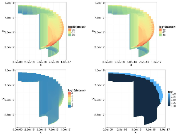
Figure 2: Observer frame simultaneous emission, absorption, intensity and optical depth that contribute to the emission at $T=1.4\times 10^{6}$ seconds at $15.4$ GHz. Top left: synchrotron emissivity in erg s^-1 cm^-3 Hz^-1. Top right: synchrotron self-absorption in cm^-1. Bottom left: specific intensity in erg s^-1 cm^-2 Hz^-1. The intensity is the result of integrating Equation 2 from bottom to top for each vertical line. Bottom right: optical depth measured from the observer (integral of the absorption from top to bottom along vertical lines). The light blue colored region denotes the part of the emitting volume that is transparent, while the emission in the dark blue region is absorbed. As explained in Section 3.2.1, the information displayed here is a subset of the data stored in the global array used by SPEV to compute the intensity in each pixel (see Section 2.2). The luminosity is obtained by integrating the intensity along vertical lines in the top right panel (taking into account that the emission is axially symmetric).

3.2.2 Off-axis light curves

Here we comment on the procedure we use to reduce the numerical noise that shows at early times (Figure 1). As was commented in Section 3.1, the jet is small at early times, so that at a typical resolution of $1000$ points per spatial direction it is very poorly resolved by the VD. Due to memory limitations we were not able to use VD resolution of $10000^{2}$. However, the resolutions of $1000^{2}$ pixels were feasible. Therefore, we adopted the following procedure:

1. Pre-determine the jet viewing angle $\theta_{\rm obs}$ and the times $T_{i}$ ($i=1,\ ..\ n_{t}$) at which it is to be observed.

2. Compute the radio images using $1000\times 1000$ VD for each $T_{i}$ in a single calculation.

3. For each $T_{i}$, determine the rectangle that contains $99.99\%$ of the emission. Then expand the rectangle by a safety margin.

4. For each $T_{i}$, independently re-compute the radio image by limiting the VD to the rectangle computed in the previous step, but using the resolution $1000\times 1000$.

The above procedure enables us to compute the emission from early times without numerical artifacts. The tradeoff is that we need to postprocess the intermediate files multiple times: once in step (ii) and then additional $n_{t}$ times in step (iv). The computing time does not necessarily scale as $n_{t}$ since, for each $T_{i}$, the emission and absorption coefficients are only computed from those emitting volumes that contribute to the emission, while the rest (typically corresponding to most of the volume of the model) are ignored. This is made efficient by indexing the intermediate files. For a given observing angle the calculations at $8$ different observing frequencies last $\simeq 3-5$ days.

4 Summary

In this contribution we have discussed the technical details of the one and two dimensional simulations of the SwJ1644 jet. In Section 2 we explain in detail how the relativistic hydrodynamic simulations are coupled to the radiative transfer code to produce the synthetic observations (light curves) that can be directly compared to the observations. In Section 3.1 we show that many one-dimensional tests can be used to probe the sensitivity of the computed light curves on the resolution of the hydrodynamic simulations, on the frequency of stored snapshots, on the resolution of the discretization in energy space and of the virtual detector. The results obtained helped to determine the resolution of the two dimensional simulation so that its computational cost is acceptable, but also so that the final light curves are as free of numerical artifacts as possible. This procedure has been successful in enabling us to produce a viable two-component jet model of the SwJ1644 jet.

References

- [1] Lacy J H, Townes C H and Hollenbach D J ApJ 262, 120
- [2] Rees M J 1988 Nature 333, 523
- [3] Evans C R and Kochanek C S 1989 ApJ 346, 13
- [4] Strubbe L E and Quataert E 2009 MNRAS 400, 2070
- [5] Lodato G and Rossi E M 2011 MNRAS 410 359
- [6] Giannios D and Metzger B D 2011 MNRAS 416, 20102
- [7] Krolik J H and Piran T 2012 ApJ 749, 92
- [8] Tchekhovskoy A, Metzger B D, Giannios D and Kelley L Z 2014 MNRAS 437, 2744
- [9] Metzger B D, Williams P K G and Berger E 2015 ApJ 806, 224
- [10] Bloom J S et al. 2011 Science 333, 203
- [11] Burrows D N et al. 2011 Nature 476, 421
- [12] Levan A J et al. 2011 Science 333, 109
- [13] Zauderer B A et al. 2011 Nature 476, 425
- [14] Berger E et al. 2012 ApJ 748, 36
- [15] Zauderer B A et al. 2013 ApJ 767, 152
- [16] Metzger B D, Giannios D and Mimica P 2012 MNRAS 420, 3528
- [17] van Velzen S, Körding E and Falcke H 2011 MNRAS 417, L51
- [18] Mimica P, Giannios D, Metzger B D and Aloy M A 2015 MNRAS 450, 2824
- [19] Aloy M A, Ibáñez J M, Martí J M and Müller E 1999 ApJS 122, 151
- [20] Leismann T et al. 2005 A&A 436, 503
- [21] Mimica P, Giannios D and Aloy M A 2009 A&A 494, 879
- [22] Colella P and Woodward P R 1984 JCP 54, 174
- [23] Shu C W and Osher S J 1984 JCP 77, 439
- [24] Donat R, Font J A, Ibáñez J M and Marquina A 1988 JCP 146, 58
- [25] Mimica P et al. 2009 ApJ 696, 1142
- [26] Sironi S, Keshet U and Lemoine M 2015 Space Science Reviews 191, 519
- [27] Sari R, Piran T and Narayan R 1998 ApJ 49, L17
- [28] Mimica P and Aloy M A 2012 MNRAS 421, 2635
- [29] Aloy C., 2013, master’s thesis, Univ. Polit. de Valencia., https://riunet.upv.es/handle/10251/35350
- [30] Kumar P, Barniol Duran R, Bošnjak Ž and Piran T 2013 MNRAS 445, 3919