Thermodynamics of slow solutions to the Gas-Piston equations

Abstract

Despite its historical importance, a perfect gas enclosed by a pistons and in contact with a thermal reservoirs is a system still largely under study. Its thermodynamic properties are not yet well understood when driven under non-equilibrium conditions. In particular, analytic formulas that describe the heat exchanged with the reservoir are rare. In this paper we prove a power series expansions for the heat when both the external force and the reservoir temperature are slowly varying over time but the overall process is not quasi-static. To do so, we use the dynamical equations from [Cerino et al., Phys. Rev. E, 91 032128] and an uncommon application of the regular perturbation technique.

I Introduction

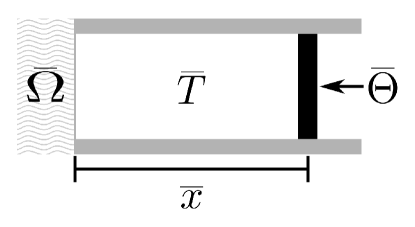
One of the main goals of non-equilibrium thermodynamics is to understand how a thermodynamic system evolves over time degrootmazur ; seifert ; sekimoto . The problem is difficult even in the simplest physical instances. For example, the non-equilibrium behavior of the adiabatic piston gruber is still a live research topic (gislason, ; abreu, ; gruber, , and references therein). Another problem which is conceptually simple, but difficult to treat is the non-equilibrium thermodynamics of a perfect gas enclosed by a cylindrical canister with a movable piston and in contact with a heat reservoir (see Figure 1). For this system there are multiple valid approaches: for example the one particle gas approachLuaGrosberg and its legacyBaule ; Hoppenau ; Gong ; Proesmans , the explicit-friction formulæ approach bizarro1 ; bizarro2 ; bizarro3 , and the gas particles-average approach vulpiani1 ; Cerino2 ; Izumida ; hisao . Among those references vulpiani1 is particularly interesting: there, the authors assumed that (i) the gas is perfect and 1-dimensional; (ii) the piston and each gas particle undergoes elastic collisions, so work is the energy exchanged in this way; (iii) the velocity of a gas particle is randomly changed according to the Maxwell-Boltzmann distribution of the reservoir when reservoir-gas particle collisions occurs tehver and heat is the change in energy of the gas; (iv) the gas distribution is always Maxwellian although gas-reservoir and gas-piston collisions change the temperature of the gas over time. Combined in a laborious averaging process, the authors where able to derive a set of dynamical equations for the time evolution of the gas temperature $\overline{T}$ and piston position $\overline{x}$ according to any externally prescribed change of the external force $\overline{\Theta}$ and reservoir temperature $\overline{\Omega}$. In ChiuchiuGubbiotti01 we showed with the multiple scales method Kuzmak1959 ; KevorkianCole ; Holmes ; BenderOrszag and some technical assumptions, (discussed in Section II) that the equations derived in vulpiani1 allows to find an approximated expression for the heat exchanged with the reservoir in two physically relevant cases: the relaxation to equilibrium and the slow isothermal compression. In the same paper ChiuchiuGubbiotti01 we pointed out the existence of particular solutions, which we called dynamical equilibrium solutions, which describe the asymptotic behavior of the system when externally driven.

Stimulated by our previous understanding, we show in this paper how to iteratively construct the dynamical equilibrium solution at any desired precision order through an uncommon application of the regular perturbation theory KevorkianCole ; Holmes ; BenderOrszag . Our only assumptions will be that both the external force and the reservoir temperature are slow, smooth and non-vanishing. Such solution immediately yields a general formula for the heat exchanged with the reservoir as a formal power series in which all the coefficients are determined. Such kind of results are important due to their rarity in the literature and we believe that the method we used can be safely applied to other relevant problems in non-equilibrium thermodynamics. We suggest that similar power series approaches can play a key role in the characterization of thermal cycles where drivings are slow but not necessarily quasi-static.

This paper is structured as follows: in Section II we introduce the model from vulpiani1 together with the notations and the formalism we will use throughout the paper; in Section III we derived our main results, namely the full recursive relation from which we can derive the coefficients of dynamical equilibrium solution and the exchanged heat; in Section IV we comment the thermodynamical relevance of our result, pointing also out similarities with the virial expansion, and make some conjectures for possible future developments.

Figure 1: A schematic representation of the gas closed by a piston and in contact with a thermal reservoir. The quantities shown in the figure are the piston position $\overline{x}$, the gas temperature $\overline{T}$, the external force $\overline{\Omega}$ and the reservoir temperature $\overline{\Theta}$.

II Background

With the list of assumptions declared in Section I, Cerino et. al. were able to derive a set of equations to describe the dynamics of a gas inside a piston under the action of a variable external force when also the reservoir temperature changes over time. Such equations are

$$\begin{aligned} \ddot{\overline{x}}&+\frac{\overline{\Theta}}{M}-\dfrac{\nu N}{\nu+1}\frac{1}{\overline{x}}\operatorname{erfc}\Big{(}\sqrt{\dfrac{m}{2\overline{T}}}\dot{\overline{x}}\Big{)}(\dot{\overline{x}}^{2}+\dfrac{\overline{T}}{m})+\dfrac{\nu N}{\nu+1}\exp\Big(-\frac{m\dot{\overline{x}}^{2}}{2\overline{T}}\Big{missing})\frac{\dot{\overline{x}}}{\overline{x}}\sqrt{\dfrac{2\overline{T}}{\pi m}}=0,\\ \end{aligned}$$ (1a)

$$\begin{aligned} \dot{\overline{T}}&+\frac{2\dot{\overline{x}}\left[m\dot{\overline{x}}^{2}+\overline{T}(1-2\nu)\right]}{\overline{x}(\nu+1)^{2}}\operatorname{erfc}\Big{(}\sqrt{\dfrac{m}{2\overline{T}}}\dot{\overline{x}}\Big{)}+\sqrt{\dfrac{2\overline{T}}{\pi m}}\frac{\overline{T}-\overline{\Omega}}{\overline{x}}+\frac{2}{\overline{x}(\nu+1)^{2}}\sqrt{\dfrac{2m\overline{T}}{\pi}}\left(\dfrac{2\nu\overline{T}}{m}-\dot{\overline{x}}^{2}\right)\exp\Big(-\frac{m\dot{\overline{x}}^{2}}{2\overline{T}}\Big{missing})=0,\end{aligned}$$ (1b)

where the upper dots denote time derivatives, $M$ is the mass of the piston, $m$ is the mass of a single gas molecule, $N$ is the total number of gas molecules, $\nu=m/M$, $\operatorname{erfc}(\cdot)$ is the complementary error function, $\overline{\Omega}$ is the externally controlled reservoir temperature, $\overline{\Theta}$ is the externally controlled force exerted on the piston, $\overline{x}$ is the piston position and $\overline{T}$ is the gas temperature. Eq.(1) give a fairly good description of both the dynamics and the thermodynamics of the system vulpiani1 , the latter being expressed through

$$\overline{E} =M\frac{\dot{\overline{x}}^{2}}{2}+\overline{\Theta}\ \overline{x}+\frac{N\overline{T}}{2},$$ (2a)

$$\overline{Q}(\overline{t}_{i},\overline{t}_{f}) =-\int_{\overline{t}_{i}}^{\overline{t}_{f}}\bigg{[}\overline{\Theta}\dot{\overline{x}}+M\dot{\overline{x}}\ \ddot{\overline{x}}+\frac{N}{2}\dot{\overline{T}}\bigg{]}\,\mathrm{d}\overline{t}.$$ (2b)

where $\overline{E}$ is the total energy of the system jarzynski2 (composed by the kinetic energy of the piston, by the linear potential energy related to $\overline{\Theta}$ and by the thermal energy of the 1-Dimensional gas respectively), and $\overline{Q}$ is the heat seifert that the system exchanges with the reservoir. In (ChiuchiuGubbiotti01, ) we showed that the thermodynamic limit

$$\frac{m}{M}=\nu\to 0,\quad N\to\infty,\quad\varepsilon=\sqrt{\frac{Nm}{M}}=\mbox{constant}$$ (3)

can be taken in eq.(1) if we first adimension them with the following transformation

$$\overline{x} =x\cdot\frac{\Omega_{r}N}{\Theta_{r}(1+\nu)g(\nu)}$$ (4a)

$$\overline{T} =T\cdot\frac{\Omega_{r}}{g(\nu)}$$ (4b)

$$\overline{\Theta} =\Theta\cdot\Theta_{r}$$ (4c)

$$\overline{\Omega} =\Omega\cdot\Omega_{r}$$ (4d)

$$\overline{t} =\frac{t}{\Theta_{r}}\cdot\sqrt{\frac{mN\Omega_{r}}{\nu(1+\nu)g(\nu)}}$$ (4e)

where

$$g(\nu)=\frac{1+6\nu+\nu^{2}}{(1+\nu)^{2}}$$ (5)

and $\Theta_{r}$ ($\Omega_{r}$) is an arbitrary force (temperature) reference value. Using these substitutions and then taking the thermodynamic limit eq.(3) in eq.(1)-(2), we obtain the following dimensionless dynamical equations

$$\begin{aligned} \ddot{x}&+\Theta-\operatorname{erfc}\Big{(}\frac{\varepsilon\dot{x}}{\sqrt{2T}}\Big{)}\frac{\varepsilon^{2}\dot{x}^{2}+T}{x}+\exp\Big(-\frac{\varepsilon^{2}\dot{x}^{2}}{2T}\Big{missing})\frac{\dot{x}}{x}\sqrt{\dfrac{2T}{\pi}}\varepsilon=0,\end{aligned}$$ (6a)

$$\begin{aligned} \dot{T}&-2\operatorname{erfc}\Big{(}\frac{\varepsilon\dot{x}}{\sqrt{2T}}\Big{)}\frac{\dot{x}}{x}(\varepsilon^{2}\dot{x}^{2}+T)+\sqrt{\dfrac{2T}{\pi}}\frac{T-\Omega}{\varepsilon x}-2\sqrt{\dfrac{2T}{\pi}}\varepsilon\frac{\dot{x}^{2}}{x}\exp\Big(-\frac{\varepsilon^{2}\dot{x}^{2}}{2T}\Big{missing})=0.\end{aligned}$$ (6b)

with the dimensionless $E$, and $Q$ densities:

$$E= \frac{\overline{E}}{N\Omega_{r}}=\Theta x+\frac{\dot{x}^{2}}{2}+\frac{T}{2},$$ (7a)

$$Q(\overline{t}_{i},\overline{t}_{f})= \frac{\overline{Q}}{N\Omega_{r}}=-\int_{t_{i}}^{t_{f}}\bigg{[}\Theta\dot{x}+\dot{x}\ddot{x}+\frac{1}{2}\dot{T}\bigg{]}\,\mathrm{d}t.$$ (7b)

The most important feature of eq.(6) is that they involve only the ratio $\varepsilon$ of the total mass of the gas and the mass of the piston as a physical parameter, a feature that this system shares with the adiabatic piston problem gruber . Moreover, the gas has to be perfect, a condition that will likely end in having $\varepsilon$ small. As a consequence, if a perturbation parameter is required for some approximated approach, $\varepsilon$ is the most natural one to choose gruber . An additional advantage of eq.(6) is that it’s easy to check that their equilibrium condition is

$$x_{\text{eq}}=\frac{\Omega}{\Theta},\quad\dot{x}_{\text{eq}}=0,\quad T_{\text{eq}}=\Omega,$$ (8)

which is exactly what the perfect gas law and standard thermodynamics requires. If one is interested in situations where the system remains in the proximity of the equilibrium condition for $\Theta$ and $\Omega$, even if $\Theta$ and $\Omega$ changes over time, then eq.(6) can be linearized around eq.(8). This process yields the following linear dimensionless equations

$$\begin{aligned} \ddot{x}&+\frac{\Theta^{2}}{\Omega}\bigg{(}x-\frac{\Omega}{\Theta}\bigg{)}+2\sqrt{\dfrac{2}{\pi\Omega}}\varepsilon\Theta\dot{x}-\Theta\frac{T-\Omega}{\Omega}=0,\end{aligned}$$ (9a)

$$\dot{T}+2\Theta\dot{x}+\sqrt{\dfrac{2}{\pi\Omega}}\frac{\Theta}{\varepsilon}(T-\Omega)=0$$ (9b)

In ChiuchiuGubbiotti01 we assumed $\varepsilon$ to be a “small” perturbative parameter, the reservoir temperature to be constant (without loss of generality. $\Omega=1$) and the external forcing $\Theta$ to be slowly varying over time (any function $B$ can be considered “slow” if $B=B(\varepsilon t)$, which we assume from now on). With such assumptions we were able to find with the multiple scales method analytic approximated solutions to (9). In particular we showed that the relevant behavior of the system is described by the following three scales:

$$t_{0}=\frac{1}{\varepsilon}\int_{0}^{t}\Theta\left(\varepsilon\chi\right)\mathrm{d}\chi,\quad t_{1}=\int_{0}^{t}\Theta\left(\varepsilon\chi\right)\mathrm{d}\chi,\quad t_{2}=\varepsilon t,$$ (10)

where an explicit form of $\Theta$ it not required to give them an intuitive meaning. The $t_{0}$-scale is the fastest one and characterizes a transient suppression of the temperature of the gas. From a physical point of view, it describes the indirect coupling of the piston with the reservoir. The $t_{1}$-scale is the one at which transient oscillations of the system are established. This reflects the direct coupling of the gas with the piston position and velocity. In the $t_{2}$-scale the exponential suppression of the transient oscillatory terms appears and is the proper scale of the external forcing too.

The approximated solution derived in ChiuchiuGubbiotti01 falls, as $t\to\infty$, into a peculiar solution:

$$x_{\text{d.eq.}}(t)=\frac{1}{\Theta\left(\varepsilon t\right)}+\varepsilon^{2}\left[\frac{\Theta^{\prime}\left(\varepsilon t\right)}{\Theta^{4}\left(\varepsilon t\right)}-2\frac{(\Theta^{\prime})^{2}\left(\varepsilon t\right)}{\Theta^{5}\left(\varepsilon t\right)}\right.\left.+\left(2\sqrt{\frac{2}{\pi}}+\sqrt{2\pi}\right)\frac{\Theta^{\prime}\left(\varepsilon t\right)}{\Theta^{3}\left(\varepsilon t\right)}\right]+\mathcal{O}\left(\varepsilon^{4}\right)$$ (11)

with prime notation

$$B^{\prime}(s)=\left.\frac{\partial{B}(\mu)}{\partial\mu}\right|_{\mu=s}.$$ (12)

We called this solution a dynamical equilibrium solution as, from a physical point of view, it describes the system when it asymptotically follows the slow external driving. Mathematically this solution arise as the particular solution of the inhomogeneous ordinary differential equations coming from the multiple scales expansion and can be computed in practice by taking all the integration constants in the multiple scale expansion equal to zero. In ChiuchiuGubbiotti01 , we also hinted that the dynamical equilibrium solution (11) could have been obtained with the “slow” regular perturbation

$$x_{\text{d.eq.}}(t)=x_{0}(\varepsilon t)+\varepsilon x_{1}(\varepsilon t)+\varepsilon^{2}x_{2}(\varepsilon t)+\varepsilon^{3}x_{3}(\varepsilon t)+\mathcal{O}\left(\varepsilon^{4}\right).$$ (13)

In the next Section we expand this point to show the generalization of the ansatz eq.(13) allows to iteratively construct the dynamical equilibrium solution at any order when both the external force $\Theta$ and the reservoir temperature $\Omega$ are slow.

III Derivation of the dynamical equilibrium solution and of the heat

Following the same procedure we used in ChiuchiuGubbiotti01 we transform the system (9) into a single third order equation. At difference with ChiuchiuGubbiotti01 , where $\Omega\equiv 1$, we assume that the external force and the reservoir temperatures are slow, i.e. $\Theta=\Theta(\varepsilon t)$, $\Omega=\Omega(\varepsilon t)$. Then we solve (9a) for $T$:

$$T={\frac{\Omega\left(\varepsilon t\right)}{\Theta\left(\varepsilon t\right)}}\ddot{x}+2\sqrt{\frac{2}{\pi}}\sqrt{\Omega(\varepsilon t)}{\varepsilon}\dot{x}+\Theta\left(\varepsilon t\right)x$$ (14)

and substitute in eq. (9b) to obtain:

$$\frac{\Omega\left(\varepsilon t\right)}{\Theta\left(\varepsilon t\right)}\dddot{x} +\left[2{\frac{\sqrt{\Omega\left({\varepsilon}t\right)}\sqrt{2}{\varepsilon}}{\sqrt{\pi}}}-{\frac{\Omega\left({\varepsilon}t\right)\Theta^{\prime}\left({\varepsilon}t\right){\varepsilon}}{\Theta^{2}\left({\varepsilon}t\right)}}+{\frac{\Omega^{\prime}\left({\varepsilon}t\right){\varepsilon}}{\Theta\left({\varepsilon}t\right)}}+{\frac{\sqrt{\Omega\left({\varepsilon}t\right)}\sqrt{2}}{\sqrt{\pi}{\varepsilon}}}\right]\ddot{x}$$ (15)

$$+\left[3\Theta\left({\varepsilon}t\right)+{\frac{\sqrt{2}{{\varepsilon}}^{2}\Omega^{\prime}\left({\varepsilon}t\right)}{\sqrt{\pi}\sqrt{\Omega\left({\varepsilon}t\right)}}}+4{\frac{\Theta\left({\varepsilon}t\right)}{\pi}}\right]\dot{x}+\left[\Theta^{\prime}\left({\varepsilon}t\right){\varepsilon}+{\frac{\sqrt{2}\left(\Theta\left({\varepsilon}t\right)\right)^{2}}{\sqrt{\pi}{\varepsilon}\sqrt{\Omega\left({\varepsilon}t\right)}}}\right]x-{\frac{\sqrt{2}\Theta\left({\varepsilon}t\right)\sqrt{\Omega\left({\varepsilon}t\right)}}{\sqrt{\pi}{\varepsilon}}}=0.$$

Now, instead of looking for a general approximation of $x(t)$ with the multiple scale method, we limit ourselves to the search for dynamical equilibrium solution $x_{\text{d.eq.}}(t)$. To this end we must get rid of transient-like behaviors, i.e. those governed by the $t_{0}$ and $t_{1}$ scales in (10). The observation in ChiuchiuGubbiotti01 that the dynamical equilibrium solution (11) is obtainable from the ansatz (13) suggests us to consider the following expansion:

$$x_{\text{d.eq.}}(t)=\sum_{n=0}^{\infty}x_{n}(\varepsilon t)\varepsilon^{n}.$$ (16)

The series (16) is a regular perturbation expansion with an uncommon feature: its coefficients are functions of the slowest time scale $t_{2}$ in (10). With this choice all transient-like behaviors are automatically ruled out, exactly as desired. We then substitute (16) in eq.(15) and, upon defining

$$s=\varepsilon t,$$ (17)

isolating $\varepsilon$ coefficient, and then equating them to zero we obtain a system of linear algebraic equations for $x_{n}(s)$. Solving it, we find:

$$x_{0}(s) =\frac{\Omega\left(s\right)}{\Theta\left(s\right)},$$ (18a)

$$x_{1}(s) =0,$$ (18b)

$$x_{2}(s) \begin{aligned} &={\sqrt{\frac{2}{\pi}}\left(\pi+2\right)\frac{\Theta^{\prime}\left(s\right)\Omega^{3/2}\left(s\right)}{\Theta^{3}\left(s\right)}}-{\frac{\Omega^{\prime\prime}\left(s\right)\Omega\left(s\right)}{\Theta^{3}\left(s\right)}}\\ &+{\frac{\Omega^{2}\left(s\right)\Theta^{\prime\prime}\left(s\right)}{\Theta^{4}\left(s\right)}}-\frac{1}{2}\sqrt{\frac{2}{\pi}}\left(3\pi+4\right){\frac{\sqrt{\Omega(s)}\Omega^{\prime}\left(s\right)}{\Theta^{2}\left(s\right)}}\\ &+2{\frac{\Omega\left(s\right)\Theta^{\prime}\left(s\right)\Omega^{\prime}\left(s\right)}{\Theta^{4}\left(s\right)}}-2{\frac{\Omega^{2}\left(s\right)\left(\Theta^{\prime}\right)^{2}\left(s\right)}{\Theta^{5}\left(s\right)}},\end{aligned}$$ (18c)

$$x_{3}(s) =0,$$ (18d)

$$x_{n}(s) =L_{2}x_{n-2}+L_{4}x_{n-4},\quad n\geq 4,$$ (18e)

where $L_{2}$ and $L_{4}$ are the linear differential operators:

$$L_{2} =-{\frac{\Omega\left(s\right)\left(s\right)}{\Theta^{2}\left(s\right)}}\derivative[2]{s}-\sqrt{\frac{1}{2\pi}}{\frac{\sqrt{\Omega\left(s\right)}\left(3\pi+4\right)}{\Theta\left(s\right)}}\derivative{s}-\sqrt{\frac{\pi}{2}}{\frac{\Theta^{\prime}\left(s\right)\sqrt{\Omega\left(s\right)}}{\Theta^{2}\left(s\right)}}$$ (19a)

$$L_{4} =-\sqrt{\frac{\pi}{2}}{\frac{\Omega^{3/2}\left(s\right)}{\Theta^{3}\left(s\right)}}\derivative[3]{s}-{\frac{\Omega^{\prime}\left(s\right)}{\Theta^{2}\left(s\right)}}\derivative{s}-\left[\frac{2\Omega\left(s\right)}{\Theta^{2}\left(s\right)}+\sqrt{\frac{\pi}{2}}\frac{\sqrt{\Omega\left(s\right)}}{\Theta^{2}\left(s\right)}\left(\frac{\Omega}{\Theta}\right)^{\prime}\left(s\right)\right].$$ (19b)

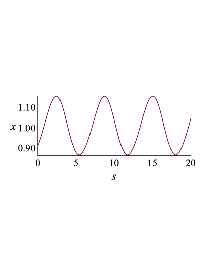
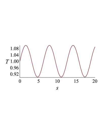
Eq.(18e) defines a recurrence relation where $x_{0}(s)$, $x_{1}(s)$, $x_{2}(s)$ and $x_{3}(s)$ act as initial conditions. We can therefore use eq.(18) and eq.(19) to obtain every term in the series (16) simply by differentiation and multiplication. Furthermore, eq.(18e) is homogeneous and $x_{1}=x_{3}=0$, then $x_{2n+1}=0$ for every $n\in\mathbb{N}$. A sample plot of $x_{\text{d.eq.}}(t)$ and the corresponding $T_{\text{d.eq.}}(t)$ with

$$\Omega(s)=1+\frac{1}{10}\sin(s),\quad\Theta(s)=1+\frac{1}{10}\cos(s)$$ (20)

is shown in Figure(2).

Figure 2: Sample trajectories for $\varepsilon=1/16$ with the first three non-zero terms of $x$ and $T$ expansions for ${\Omega(s)=1+0.1\sin(s)}$ and $\Theta(s)=1+0.1\cos(s)$.

Knowing the terms of the expansion (16), we can find an analogous series expansion for the the heat:

$$Q(0,s)=\sum_{n=0}^{\infty}Q_{2n}(0,s)\varepsilon^{2n}.$$ (21)

Indeed, substituting eq.(17) into (7b) we first find:

$$Q(0,s)= -\int_{0}^{s}\Theta(s)x^{\prime}(\sigma)\mathrm{d}\sigma-\frac{\varepsilon^{2}}{2}\left[x^{\prime}(s)-x^{\prime}(0)\right]$$ (22)

$$-\frac{T(s)-T(0)}{2}$$

which, upon the substitution of (16) and (14), yields the following values for the coefficients in (21):

$$Q_{0}(0,s) =\Theta\left(s\right)\left[x_{0}\left(0\right)-x_{0}\left(s\right)\right]-\int_{0}^{s}\!\Theta\left(\sigma\right)x_{0}^{\prime}\left(\sigma\right)\mathrm{d}\sigma$$ (23a)

$$Q_{2n}(0,s) \begin{aligned} =&-\int_{0}^{s}\Theta\left(\sigma\right)x_{2n}^{\prime}(\sigma)\mathrm{d}\sigma-\frac{1}{2}\sum_{l=0}^{n-1}\left[x^{\prime}_{2l}(s)x^{\prime}_{2n-2l-2}(s)-x^{\prime}_{2l}(0)x^{\prime}_{2n-2l-2}(0)\right]-\left[\Theta(s)x_{2n}(s)-\Theta(0)x_{2n}(0)\right]\\ &-2\sqrt{\frac{2}{\pi}}\left[\sqrt{\Omega(s)}x^{\prime}_{2n-2}(s)-\sqrt{\Omega(0)}x^{\prime}_{2n-2}(0)\right]-\left[\frac{\Omega}{\Theta}(s)x^{\prime\prime}_{2n-2}(s)-\frac{\Omega}{\Theta}(0)x^{\prime\prime}_{2n-2}(0)\right].\end{aligned}$$ (23b)

It is worth to note that all the coefficients (23) can, in principle, be determined from the recurrence relation for $x_{n}$ (18). An integration is involved, which may be non-trivial, but, from a formal point of view, the series is well defined for sufficiently small values of $\varepsilon$.

IV Discussion

In this concluding section, we comment the relevance of eq.(18) and of eq.(23) and point out interesting features. Speaking specifically of the dynamical equilibrium solution, eq.(18) possess remarkable properties. The first one is that,it allows to calculate the dynamical equilibrium solution $x_{\text{d.eq.}}$ and hence $T$ via (14) with an arbitrary precision. Only multiplications and differentiations are required in such formula, thus making the evaluation of $x$ and $T$ a trivial task. For practical purposes, the evaluation of the series (16) must be truncated at some point. Being absent the odd terms, if we stop at the $N$th iteration we will have an error of order $\mathcal{O}\left(\varepsilon^{2N+2}\right)$, which gives us a pretty high precision with few iterations. Obviously this is valid only within the convergence radius; this can be in principle determined from the recurrence relation (18e), but its determination is a complex task far beyond the scope of this paper.

The second remarkable property is that (18e) is valid for general instances of $\Theta$ and $\Omega$ provided, that they (i) depend on time only through $\varepsilon t$, (ii) they are smooth and (iii) never vanish. This last condition must necessary hold for $\Theta$, while it can be slightly relaxed for $\Omega$. A priori the vanishing of both $\Theta$ and $\Omega$ introduces singularities in eq.(15). As eqs.(18,19) show, we can’t get rid of the singularities introduced by $\Theta$. Conversely from the same equations we see that the singularities in $\Omega$ do not explicitly appear in the solution, so they are in a certain sense removable. However the price to pay is that the solution is compelled to live in a compact subset of the real line: if there exists a $s_{0}>0$ such that $\Omega(s_{0})=0$ then our solution is defined only on the subset $0\leq s<s_{0}$ due to the presence of square roots in eqs.(18,19). Physically $\Omega(s_{0})=0$ means that we allow the reservoir temperature to reach the absolute zero in a finite time, which is forbidden by thermodynamics as it means that all the degrees of freedom of the system becomes frozen. As a consequence a vanishing $\Omega(s)$ is mathematically acceptable (even if with some limitations), but clearly not physically.

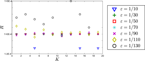
The third interesting feature of eq.(16) is that it extends the results of our previous paper ChiuchiuGubbiotti01 where we were limited to use $\Omega=1$ and opens the possibility to study thermodynamic cycles. In turn, using this regular expansion technique, we lost the characterization of transient phenomena. This is not a major drawback, if for example one is interested in the study of the thermodynamic cycles efficiency, where transient behaviors are neglected. Moreover numerical evidence lead us to conjecture that, for $\varepsilon$ sufficiently small, all solutions of (9) will at some time fall into our dynamical equilibrium solution. One example of such evidence is obtained as follows: using the particular form of $\Theta$ and $\Omega$ given in eq.(20) we simulate eq.(15) with $x(0)=x_{\text{d.eq.}}(0)$ and $x(0)=x_{\text{d.eq.}}(0)+K\varepsilon$, thus obtaining $x^{\text{num}}(t)$ and $x^{\text{num}}_{\text{d.eq.}}(t)$ respectively. We then study

$$R=\frac{\displaystyle\max_{s\in[7\pi,9\pi]}\left|x^{\text{num}}(s)-x_{\text{d.eq.}}(s)\right|}{\displaystyle\max_{s\in[7\pi,9\pi]}\left|x^{\text{num}}_{\text{d.eq.}}(s)-x_{\text{d.eq.}}(s)\right|}$$ (24)

as a function of $K$ and $\varepsilon$, where $x_{\text{d.eq.}}$ is truncated at $n=4$ and $s\in[7\pi,9\pi]$ ensures that we are way ahead of the time evolution of the system. As it emerges by Figure 3, $R\approx 1$ for various value of $N$ and $\varepsilon$, so , we reasonably say that $x^{\text{num}}(s)$ is attracted by eq.(16). This means that the dynamical equilibrium solution has a quite general usefulness.

Figure 3: Plot of $R$ as a function of $K$ for different values of $\varepsilon$.

The last interesting feature of the expansion (16) is that if we limit ourselves to the $0$-th order term, we obtain the law of perfect gasses. Higher orders terms are small corrections arising from the fact that $\Omega$ and $\Theta$ are changed in a finite time. In this sense eq.(16) and eq.(18) can be qualitatively considered as an analogue of the virial expansion for a perfect gas where finite time-effects plays the role of inter-particle interaction contributions. Clearly, this analogy is a formal one: in vulpiani1 the gas is assumed to be perfect and remains perfect during the whole time evolution. However it is not unreasonable to think that the corresponding equation will have as $0$-th order term the usual virial theorem for real gasses if the gas particles are allowed to interact. This suggests the existence of higher order time-dependent virial theorems.

Coming to the relevance of (21) and (23), they allow us to calculate the heat as a formal series in which all the coefficients are well determined through a purely mechanical model vulpiani1 . Eq.(23) is therefore a quite uncommon result in the framework of non-equilibrium thermodynamics, as similar formal results are rare in the literatur. It gives an explicit expression of heat exchanged at any intermediate time that can be evaluated a priori with the sole knowledge of the driving protocol. This opens interesting scenarios to analyze. For example it reduces the evaluation of heat in practice to the problem of finding the terms in (16) and to performing the integration in eq.(23). Another interesting possibility is the formal evaluation of the efficiency of thermodynamic cycles when drivings are slow but not necessarily quasi-static, i.e. to characterize situations where efficiency is expected to be high while the power is close to zero. We point out that in the original model we are not allowed to consider adiabatic transformations. Therefore we are unable to describe Carnot cycles but it is possible to study Ericsson-like cyclesvulpiani1 ; Cerino2 , with the only caveat that $\Omega$ and $\Theta$ must be smooth function. This may seems an internal contradiction as Ericsson cycle is not smooth; however, any periodic functions can be reasonably approximated by a smooth trigonometric polynomialWhittaker . To satisfy the “slow” driving condition such trigonometric polynomial should not contain high order harmonics, but this is usually sufficient to yield a good approximation.