Cooling a Mechanical Resonator to Quantum Regime by heating it

Yue Ma Center for Quantum Information, Institute for Interdisciplinary Information Sciences, Tsinghua University, Beijing 100084, China Department of Physics, Tsinghua University, Beijing 100084, China    Zhang-qi Yin yinzhangqi@mail.tsinghua.edu.cn Center for Quantum Information, Institute for Interdisciplinary Information Sciences, Tsinghua University, Beijing 100084, China    Pu Huang Hefei National Laboratory for Physics Sciences at Microscale and Department of Modern Physics, University of Science and Technology of China, Hefei 230026, China    W. L. Yang State Key Laboratory of Magnetic Resonance and Atomic and Molecular Physics, Wuhan Institute of Physics and Mathematics, Chinese Academy of Sciences, Wuhan 430071, China    Jiangfeng Du djf@ustc.edu.cn Hefei National Laboratory for Physics Sciences at Microscale and Department of Modern Physics, University of Science and Technology of China, Hefei 230026, China
Abstract

We consider a mechanical resonator made of diamond, which contains a nitrogen-vacancy center (NV center) locating at the end of the oscillator. A second order magnetic gradient is applied and inducing coupling between mechanical modes and the NV center. By applying proper external magnetic field, the energy difference between NV center electron spin levels can be tuned to match the energy difference between two mechanical modes a𝑎a and b𝑏b. A laser is used for continuously initializing the NV center electron spin. The mode a𝑎a with lower frequency is driven by a thermal bath. We find that the temperature of the mode b𝑏b is significantly cooled when the heating bath temperature is increased. We discuss the conditions that quantum regime cooling requires, and confirm the results by numerical simulation. Finally we give the intuitive physical explanation on this unusual effect.

Composite Quantum System; Thermal Phonon Bath; NV Center; Mechanical Resonator; Cooling
pacs:
******

I introduction

Cooling and manipulating the motion of mechanical resonator is widely studied now ASP2014 . It has many applications in quantum information science Regal2011 ; Barzanjeh2012 ; Wang2012 ; Tian2012 ; Rips2013 ; Yin2009a ; Yin2015a ; Barzanjeh2015 , testing quantum effects in macroscopic systems PEN1996 ; Connell2010 ; Teufel2011 ; Poot2012 ; Pikovski2012 ; NIM2013 ; Bassi2013 ; Isart2011 ; Yin2013 ; Li2016 ; Barzanjeh2016 , ultra-sensitive sensing Caves1981 ; Geraci2010 ; Yin2011 ; Arvanitaki2013 ; Huang2013 ; Zhao2014 , etc. In order to cool mechanical resonator, we should couple it to other cold systems such as cavity mode (optomechanics) sideband1 ; sideband2 ; Liu2013 , electronic spin (Nitrogen-vacancy centers) RAB2009 ; MacQuarrie2016 ; Li2016b , etc. In optomechanics, laser cooling of mechanical resonators is a typical method. Intuitively, this is not hard to understand. A laser produces coherent light, which is well ordered (cold), and will make the mechanical system couple with a colder cavity bath sideband1 ; sideband2 . However, counter-intuitively, recent research showed that a thermal light, which is very hot , can also cool an opto-mechanical system MAR2012 . In this system, the mechanical resonator to be cooled is coupled with two optical modes Yin2009 . The low frequency mode is in contact with a hot thermal light while the high frequency mode is not, acting as an auxiliary part. After the system reaches the equilibrium state, the thermal phonon number in the mechanical mode will be smaller.

In a hybrid system that contains a NV center and a mechanical resonator, a magnetic gradient is applied to couple the NV center with the resonator. The NV center is continuously initialized by a laser, and could be used for cooling the mechanical resonator to the ground state RAB2009 . In previous literatures, the first order magnetic gradient was used for inducing coupling between the NV center and the mechanical mode RAB2009 ; YIN2015 ; Zhou2010 ; Xu2009 ; Chen2010 ; Arcizet2011 ; Kolkowitz2012 . It is quite naturally to ask whether the higher order magnetic gradient could be useful for coupling the NV center and the mechanical resonator and cooling it.

In this paper, we consider system that contains a mechanical cantilever and a NV center YIN2015 . A second order magnetic gradient is applied to induce the coupling between NV center and the two mechanical modes a𝑎a and b𝑏b. The electron spin transition frequency of the NV center is tuned to match the mechanical modes frequencies difference. The NV center is continuously resetted to the ground state by a laser. In this way, the NV center acts as an effective vacuum bath to cool the mode b𝑏b. An incoherent driving (thermal bath) is applied on the lower frequency mode a𝑎a, and resulting a higher temperature of it. The incoherent driving on mode a𝑎a also increases the effective coupling between mode b𝑏b and the NV center, and cools the mode b𝑏b. We find that the quantum regime cooling is possible under the current experimental conditions.

The paper is orgnized as follows. In section II, we introduce the scheme of the second order magnetic field gradient induced coupling between NV center and mechanical modes. In section III, we derived the analytical solution for the system. In Section IV, the analytical results are verified by numerical simulation. In section V, a discussion and conclusion are given.

II The scheme

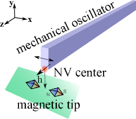
As shown in Fig. 1, we consider a diamond cantilever resonator that contains a NV center at the end of it. Two mechanical modes a𝑎a and b𝑏b are under consideration, with frequencies ωa<ωbsubscript𝜔𝑎subscript𝜔𝑏\omega_{a}<\omega_{b}. Two spin states of the NV center electron are relevant here, |1ket1|-1\rangle and |0ket0|0\rangle. By applying proper magnetic field, the energy split between the two states of the NV center, ωzsubscript𝜔𝑧\omega_{z}, is equal to the energy difference of the two mechanical modes, Δ=ωbωaΔsubscript𝜔𝑏subscript𝜔𝑎\Delta=\omega_{b}-\omega_{a}. Due to the second order magnetic gradient G2=2B/x2subscript𝐺2superscript2𝐵superscript𝑥2G_{2}=\partial^{2}B/\partial x^{2}, the two mechanical modes a𝑎a and b𝑏b both couple with the NV center.

Refer to caption
Figure 1: A nano-diamond is fabricated as a thin cantilever which can oscillate along the x𝑥x axis, while the defect of an NV center is at the end. Two magnetic tips, which point along the x𝑥x axis and generate second order magnetic gradient along the x𝑥x axis, are placed below the cantilever. The distance between the mid point of the connection lines of the tips and the NV center are around 505050 nm. And an external static magnetic field Bextsubscript𝐵𝑒𝑥𝑡B_{ext} is added along the z𝑧z axis to induce Zeeman split in order to drive away the NV center spin |+1ket1|+1\rangle state and keep the |0ket0|0\rangle and |1ket1|-1\rangle state closer.

Initially, both mechanical modes a𝑎a and b𝑏b are in the thermal states with the average thermal phonon number n¯asubscript¯𝑛𝑎\bar{n}_{a} and n¯bsubscript¯𝑛𝑏\bar{n}_{b}. The mode a𝑎a is driving by a thermal bath with average phonon number much higher than its environment. The NV center electron spin is initialized to the |0ket0|0\rangle state at the beginning. The Hamiltonian of the whole system can be expressed as H=H0+H1𝐻subscript𝐻0subscript𝐻1H=H_{0}+H_{1}, where H0subscript𝐻0H_{0} is the non-interaction part and H1subscript𝐻1H_{1} describes the interaction between the mechanical resonator and the NV center electron spin.

H0subscript𝐻0\displaystyle H_{0} =ωz2σz+ωaaa+ωbbbabsentsubscript𝜔𝑧2subscript𝜎𝑧subscript𝜔𝑎superscript𝑎𝑎subscript𝜔𝑏superscript𝑏𝑏\displaystyle=\frac{\omega_{z}}{2}\sigma_{z}+\omega_{a}a^{\dagger}a+\omega_{b}b^{\dagger}b (1)
H1subscript𝐻1\displaystyle H_{1} =(gaaa+gbbb+gab(ab+ab))σxabsentsubscript𝑔𝑎superscript𝑎𝑎subscript𝑔𝑏superscript𝑏𝑏subscript𝑔𝑎𝑏superscript𝑎𝑏𝑎superscript𝑏subscript𝜎𝑥\displaystyle=\left(g_{a}a^{\dagger}a+g_{b}b^{\dagger}b+g_{ab}(a^{\dagger}b+ab^{\dagger})\right)\sigma_{x}

where ga=gsμBG2xa2subscript𝑔𝑎subscript𝑔𝑠subscript𝜇𝐵subscript𝐺2superscriptsubscript𝑥𝑎2g_{a}=g_{s}\mu_{B}G_{2}x_{a}^{2}, gb=gsμBG2xb2subscript𝑔𝑏subscript𝑔𝑠subscript𝜇𝐵subscript𝐺2superscriptsubscript𝑥𝑏2g_{b}=g_{s}\mu_{B}G_{2}x_{b}^{2}, and gab=gsμBG2xaxbsubscript𝑔𝑎𝑏subscript𝑔𝑠subscript𝜇𝐵subscript𝐺2subscript𝑥𝑎subscript𝑥𝑏g_{ab}=g_{s}\mu_{B}G_{2}x_{a}x_{b}, and xa=/2maωasubscript𝑥𝑎Planck-constant-over-2-pi2subscript𝑚𝑎subscript𝜔𝑎x_{a}=\sqrt{\hbar/2m_{a}\omega_{a}} (xb=/2mbωb)subscript𝑥𝑏Planck-constant-over-2-pi2subscript𝑚𝑏subscript𝜔𝑏(x_{b}=\sqrt{\hbar/2m_{b}\omega_{b}}) is the zero field fluctuation for the mechanical mode a𝑎a (b)𝑏(b), masubscript𝑚𝑎m_{a} (mbsubscript𝑚𝑏m_{b}) is the effective mass for mode a𝑎a (b𝑏b). Experimentally, ωz2π×107Hzsimilar-tosubscript𝜔𝑧2𝜋superscript107Hz\omega_{z}\sim 2\pi\times 10^{7}\ \rm{Hz}, ga,gb,gab2π×1Hzsimilar-tosubscript𝑔𝑎subscript𝑔𝑏subscript𝑔𝑎𝑏2𝜋1Hzg_{a},g_{b},g_{ab}\sim 2\pi\times 1\ \rm{Hz} can be realized (see Appendix).

Under the rotating wave approximation which shift the energy zero point by ωa(aa+bb)subscript𝜔𝑎superscript𝑎𝑎superscript𝑏𝑏\omega_{a}(a^{\dagger}a+b^{\dagger}b), we can change H0subscript𝐻0H_{0} into

H0=ωz2σz+Δbbsuperscriptsubscript𝐻0subscript𝜔𝑧2subscript𝜎𝑧Δsuperscript𝑏𝑏H_{0}^{\prime}=\frac{\omega_{z}}{2}\sigma_{z}+\Delta b^{\dagger}b (2)

Unavoidably, the system will go through some intrinsic loss. The mechanical decay γasubscript𝛾𝑎\gamma_{a} and γbsubscript𝛾𝑏\gamma_{b} is in the order of 2π×1Hz2𝜋1Hz2\pi\times 1\ \rm{Hz} (see Appendix). The intrinsic decay rate Γ0subscriptΓ0\Gamma_{0} for NV center is much less than 111 Hz at low temperature. By adding initializing laser, the decay rate ΓΓ\Gamma for the NV center electron spin would be much larger than the decay rates for the mechanical modes γasubscript𝛾𝑎\gamma_{a} and γbsubscript𝛾𝑏\gamma_{b}. The dephasing of NV center is neglected, as it could be eliminated by continuous dynamical decoupling Cai2012 . However, as we will use the same model to describe the decay of the spin and the vibration, here we should make sure that Γ,γa,γbωzmuch-less-thanΓsubscript𝛾𝑎subscript𝛾𝑏subscript𝜔𝑧\Gamma,\gamma_{a},\gamma_{b}\ll\omega_{z}. As the evolution of the system contains decay and damping, it is convenient to describe it with quantum master equation OPS , which can be written out explicitly as

ρ˙˙𝜌\displaystyle\dot{\rho} =i[H,ρ]+(a+b+s)ρabsent𝑖𝐻𝜌subscript𝑎subscript𝑏subscript𝑠𝜌\displaystyle=-i[H,\rho]+(\mathcal{L}_{a}+\mathcal{L}_{b}+\mathcal{L}_{s})\rho (3)
asubscript𝑎\displaystyle\mathcal{L}_{a} =(1+n¯a)γaDa+n¯aγaDaabsent1subscript¯𝑛𝑎subscript𝛾𝑎subscript𝐷𝑎subscript¯𝑛𝑎subscript𝛾𝑎subscript𝐷superscript𝑎\displaystyle=(1+\bar{n}_{a})\gamma_{a}D_{a}+\bar{n}_{a}\gamma_{a}D_{a^{\dagger}}
bsubscript𝑏\displaystyle\mathcal{L}_{b} =(1+n¯b)γbDb+n¯bγbDbabsent1subscript¯𝑛𝑏subscript𝛾𝑏subscript𝐷𝑏subscript¯𝑛𝑏subscript𝛾𝑏subscript𝐷superscript𝑏\displaystyle=(1+\bar{n}_{b})\gamma_{b}D_{b}+\bar{n}_{b}\gamma_{b}D_{b^{\dagger}}
ssubscript𝑠\displaystyle\mathcal{L}_{s} =ΓDσabsentΓsubscript𝐷subscript𝜎\displaystyle=\Gamma D_{\sigma_{-}}

Dxsubscript𝐷𝑥D_{x} refers to the notation in Lindblad form, which is Dx(ρ)=2xρxxxρρxxsubscript𝐷𝑥𝜌2𝑥𝜌superscript𝑥superscript𝑥𝑥𝜌𝜌superscript𝑥𝑥D_{x}(\rho)=2x\rho x^{\dagger}-x^{\dagger}x\rho-\rho x^{\dagger}x. The Eq.(3) will be solved in both analytical and numerical methods. The results of the both methods will be compared and discussed.

III Analytical Solution

As mentioned above, the phonon bath for mode a𝑎a is very large, so the average phonon number of mode a𝑎a is almost always equal to the average phonon number in the bath, that is, aa=n¯adelimited-⟨⟩superscript𝑎𝑎subscript¯𝑛𝑎\langle a^{\dagger}a\rangle=\bar{n}_{a}. Moreover, as the phonon number of mode b𝑏b is much smaller than that of mode a𝑎a, it is safe to drop the term bbsuperscript𝑏𝑏b^{\dagger}b in H1subscript𝐻1H_{1}. If we denote δ=aan¯a𝛿superscript𝑎𝑎subscript¯𝑛𝑎\delta=a^{\dagger}a-\bar{n}_{a} as the phonon occupation number fluctuation of mode a𝑎a, under the rotating wave picture, H1subscript𝐻1H_{1} can be simplified to

H1=gaδ(σ++σ)+gab(abσ++abσ)superscriptsubscript𝐻1subscript𝑔𝑎𝛿subscript𝜎subscript𝜎subscript𝑔𝑎𝑏superscript𝑎𝑏subscript𝜎𝑎superscript𝑏subscript𝜎H_{1}^{\prime}=g_{a}\delta(\sigma_{+}+\sigma_{-})+g_{ab}(a^{\dagger}b\sigma_{+}+ab^{\dagger}\sigma_{-}) (4)

For the convenience of the notation, here we rename H0H0superscriptsubscript𝐻0subscript𝐻0H_{0}^{\prime}\rightarrow H_{0}, H1H1superscriptsubscript𝐻1subscript𝐻1H_{1}^{\prime}\rightarrow H_{1}.

Using standard method of quantum master equation QNO , and after adiabatically eliminating the mode a𝑎a Yin2007 ; Yang2015 , we can get the reduced master equation for mode b𝑏b and the electron spin mode s𝑠s (see Appendix)

ρ˙b,s(t)=subscript˙𝜌𝑏𝑠𝑡absent\displaystyle\dot{\rho}_{b,s}(t)= i[H0,ρb,s(t)]+bρb,s(t)+sρb,s(t)𝑖subscript𝐻0subscript𝜌𝑏𝑠𝑡subscript𝑏subscript𝜌𝑏𝑠𝑡subscript𝑠subscript𝜌𝑏𝑠𝑡\displaystyle-i[H_{0},\rho_{b,s}(t)]+\mathcal{L}_{b}\rho_{b,s}(t)+\mathcal{L}_{s}\rho_{b,s}(t) (5)
+1ρb,s(t)+2ρb,s(t)subscript1subscript𝜌𝑏𝑠𝑡subscript2subscript𝜌𝑏𝑠𝑡\displaystyle+\mathcal{L}_{1}\rho_{b,s}(t)+\mathcal{L}_{2}\rho_{b,s}(t)

where we have introduced two new Liouvillians for convenience

1subscript1\displaystyle\mathcal{L}_{1} =gab2γa+γb+Γ((1+n¯a)Dbσ++n¯aDbσ)absentsuperscriptsubscript𝑔𝑎𝑏2subscript𝛾𝑎subscript𝛾𝑏Γ1subscript¯𝑛𝑎subscript𝐷𝑏subscript𝜎subscript¯𝑛𝑎subscript𝐷superscript𝑏subscript𝜎\displaystyle=\frac{g_{ab}^{2}}{\gamma_{a}+\gamma_{b}+\Gamma}\left((1+\bar{n}_{a})D_{b\sigma_{+}}+\bar{n}_{a}D_{b^{\dagger}\sigma_{-}}\right) (6)
2subscript2\displaystyle\mathcal{L}_{2} =(2γa+Γ)ga2(n¯a2+n¯a)ωz2+(2γa+Γ)2(Dσ++Dσ)absent2subscript𝛾𝑎Γsuperscriptsubscript𝑔𝑎2superscriptsubscript¯𝑛𝑎2subscript¯𝑛𝑎superscriptsubscript𝜔𝑧2superscript2subscript𝛾𝑎Γ2subscript𝐷subscript𝜎subscript𝐷subscript𝜎\displaystyle=\frac{(2\gamma_{a}+\Gamma)g_{a}^{2}(\bar{n}_{a}^{2}+\bar{n}_{a})}{\omega_{z}^{2}+(2\gamma_{a}+\Gamma)^{2}}(D_{\sigma_{+}}+D_{\sigma_{-}})

Eq. (6) can be written in a more compact form if we define the effective average excitation number of the NV center electron spin as

ns=(2γa+Γ)ga2(n¯a2+n¯a)Γ(ωz2+(2γa+Γ)2)superscriptsubscript𝑛𝑠2subscript𝛾𝑎Γsuperscriptsubscript𝑔𝑎2superscriptsubscript¯𝑛𝑎2subscript¯𝑛𝑎Γsuperscriptsubscript𝜔𝑧2superscript2subscript𝛾𝑎Γ2n_{s}^{\prime}=\frac{(2\gamma_{a}+\Gamma)g_{a}^{2}(\bar{n}_{a}^{2}+\bar{n}_{a})}{\Gamma\left(\omega_{z}^{2}+(2\gamma_{a}+\Gamma)^{2}\right)} (7)

In fact, nssuperscriptsubscript𝑛𝑠n_{s}^{\prime} is very close to zero because of the weak coupling requirement (gan¯a,gbn¯b,gabn¯an¯bωz)much-less-thansubscript𝑔𝑎subscript¯𝑛𝑎subscript𝑔𝑏subscript¯𝑛𝑏subscript𝑔𝑎𝑏subscript¯𝑛𝑎subscript¯𝑛𝑏subscript𝜔𝑧(g_{a}\sqrt{\bar{n}_{a}},g_{b}\sqrt{\bar{n}_{b}},g_{ab}\sqrt{\bar{n}_{a}\bar{n}_{b}}\ll\omega_{z}), in other words, due to the large energy split ωzsubscript𝜔𝑧\omega_{z} and the relative large damping rate ΓΓ\Gamma. Then we can define an effective Liouvillian for the spin as well s=s+2=(1+ns)ΓDσ+nsΓDσ+superscriptsubscript𝑠subscript𝑠subscript21superscriptsubscript𝑛𝑠Γsubscript𝐷subscript𝜎superscriptsubscript𝑛𝑠Γsubscript𝐷subscript𝜎\mathcal{L}_{s}^{\prime}=\mathcal{L}_{s}+\mathcal{L}_{2}=(1+n_{s}^{\prime})\Gamma D_{\sigma_{-}}+n_{s}^{\prime}\Gamma D_{\sigma_{+}}.

Now the equation of motion for the reduced density matrix ρb,ssubscript𝜌𝑏𝑠\rho_{b,s} becomes

ρ˙b,s(t)=i[H0,ρb,s(t)]+1ρb,s(t)+bρb,s(t)+sρb,s(t)subscript˙𝜌𝑏𝑠𝑡𝑖subscript𝐻0subscript𝜌𝑏𝑠𝑡subscript1subscript𝜌𝑏𝑠𝑡subscript𝑏subscript𝜌𝑏𝑠𝑡superscriptsubscript𝑠subscript𝜌𝑏𝑠𝑡\dot{\rho}_{b,s}(t)=-i[H_{0},\rho_{b,s}(t)]+\mathcal{L}_{1}\rho_{b,s}(t)+\mathcal{L}_{b}\rho_{b,s}(t)+\mathcal{L}_{s}^{\prime}\rho_{b,s}(t) (8)

The corresponding adjoint equations for the phonon number operator n^b=bbsubscript^𝑛𝑏superscript𝑏𝑏\hat{n}_{b}=b^{\dagger}b and excitation number operator n^s=σ+σsubscript^𝑛𝑠subscript𝜎subscript𝜎\hat{n}_{s}=\sigma_{+}\sigma_{-} can be developed then (see Appendix).

ddtn^s=𝑑𝑑𝑡subscript^𝑛𝑠absent\displaystyle\frac{d}{dt}\hat{n}_{s}= 2gab2γa+γb+Γ[(2n¯a1)n^bn^sn¯an^s\displaystyle\frac{2g_{ab}^{2}}{\gamma_{a}+\gamma_{b}+\Gamma}\Big{[}(-2\bar{n}_{a}-1)\hat{n}_{b}\hat{n}_{s}-\bar{n}_{a}\hat{n}_{s} (9)
+(n¯a+1)n^b]+2Γ[(2ns1)n^s+ns]\displaystyle+(\bar{n}_{a}+1)\hat{n}_{b}\Big{]}+2\Gamma\big{[}(-2n_{s}^{\prime}-1)\hat{n}_{s}+n_{s}^{\prime}\big{]}
ddtn^b=𝑑𝑑𝑡subscript^𝑛𝑏absent\displaystyle\frac{d}{dt}\hat{n}_{b}= 2gab2γa+γb+Γ[(2n¯a+1)n^bn^s+n¯an^s\displaystyle\frac{2g_{ab}^{2}}{\gamma_{a}+\gamma_{b}+\Gamma}\Big{[}(2\bar{n}_{a}+1)\hat{n}_{b}\hat{n}_{s}+\bar{n}_{a}\hat{n}_{s}
(n¯a+1)n^b]+2γb(n¯bn^b)\displaystyle-(\bar{n}_{a}+1)\hat{n}_{b}\Big{]}+2\gamma_{b}(\bar{n}_{b}-\hat{n}_{b})

Taking the average on both sides respect to the quantum state of the system, and under average field approximation which refers to n^bn^s=n^bn^sdelimited-⟨⟩subscript^𝑛𝑏subscript^𝑛𝑠delimited-⟨⟩subscript^𝑛𝑏delimited-⟨⟩subscript^𝑛𝑠\langle\hat{n}_{b}\hat{n}_{s}\rangle=\langle\hat{n}_{b}\rangle\langle\hat{n}_{s}\rangle, the stationary state for the average phonon number of mode b𝑏b can be solved from the quadratic equation below after we drop the nonphysical solution.

An^b2+Bn^b+C=0𝐴superscriptdelimited-⟨⟩subscript^𝑛𝑏2𝐵delimited-⟨⟩subscript^𝑛𝑏𝐶0A\langle\hat{n}_{b}\rangle^{2}+B\langle\hat{n}_{b}\rangle+C=0 (10)

where

A=𝐴absent\displaystyle A= γbgab2(2n¯a+1)γa+γb+Γsubscript𝛾𝑏superscriptsubscript𝑔𝑎𝑏22subscript¯𝑛𝑎1subscript𝛾𝑎subscript𝛾𝑏Γ\displaystyle\frac{-\gamma_{b}g_{ab}^{2}(2\bar{n}_{a}+1)}{\gamma_{a}+\gamma_{b}+\Gamma} (11)
B=𝐵absent\displaystyle B= gab2γa+γb+Γ(2n¯an¯bγb+n¯bγbn¯aγb\displaystyle\frac{g_{ab}^{2}}{\gamma_{a}+\gamma_{b}+\Gamma}(2\bar{n}_{a}\bar{n}_{b}\gamma_{b}+\bar{n}_{b}\gamma_{b}-\bar{n}_{a}\gamma_{b}
Γn¯aΓnsΓ)γbΓ(2ns+1)\displaystyle-\Gamma\bar{n}_{a}-\Gamma n_{s}^{{}^{\prime}}-\Gamma)-\gamma_{b}\Gamma(2n_{s}^{\prime}+1)
C=𝐶absent\displaystyle C= gab2γa+γb+Γn¯a(γbn¯b+Γns)+γbn¯bΓ(2ns+1)superscriptsubscript𝑔𝑎𝑏2subscript𝛾𝑎subscript𝛾𝑏Γsubscript¯𝑛𝑎subscript𝛾𝑏subscript¯𝑛𝑏Γsuperscriptsubscript𝑛𝑠subscript𝛾𝑏subscript¯𝑛𝑏Γ2superscriptsubscript𝑛𝑠1\displaystyle\frac{g_{ab}^{2}}{\gamma_{a}+\gamma_{b}+\Gamma}\bar{n}_{a}(\gamma_{b}\bar{n}_{b}+\Gamma n_{s}^{\prime})+\gamma_{b}\bar{n}_{b}\Gamma(2n_{s}^{\prime}+1)

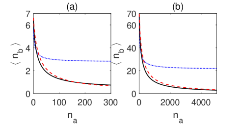
In Fig. 2, the stationary phonon number of mode b𝑏b is plotted as a function of the average phonon number of mode a𝑎a. Unlike the previous Ref. MAR2012 , where there was an optimal heating bath temperature, here increasing heating bath temperature will always cooling the resonator, which is an outstanding property. As environment temperature increase, the quantum regime cooling n^b<1delimited-⟨⟩subscript^𝑛𝑏1\langle\hat{n}_{b}\rangle<1 can be realized by increasing both the mode a𝑎a temperature and NV center decay ΓΓ\Gamma.

Refer to caption
Figure 2: n^bdelimited-⟨⟩subscript^𝑛𝑏\langle\hat{n}_{b}\rangle as a function of n¯asubscript¯𝑛𝑎\bar{n}_{a}. The parameters related to frequency are: ωz/2π=2×107subscript𝜔𝑧2𝜋2superscript107\omega_{z}/2\pi=2\times 10^{7} Hz, ga/2π=3subscript𝑔𝑎2𝜋3g_{a}/2\pi=3 Hz, gb/2π=1subscript𝑔𝑏2𝜋1g_{b}/2\pi=1 Hz, gab/2π=3subscript𝑔𝑎𝑏2𝜋3g_{ab}/2\pi=\sqrt{3} Hz, γa/2π=γb/2π=1subscript𝛾𝑎2𝜋subscript𝛾𝑏2𝜋1\gamma_{a}/2\pi=\gamma_{b}/2\pi=1 Hz. (a) The initial temperature of mode b𝑏b is 10.810.810.8 mK. The average phonon number is approximated by the Bose distribution n¯b=1/(eωbkBT1)=7subscript¯𝑛𝑏1superscript𝑒Planck-constant-over-2-pisubscript𝜔𝑏subscript𝑘𝐵𝑇17\bar{n}_{b}=1/(e^{\frac{\hbar\omega_{b}}{k_{B}T}}-1)=7. Three values of Γ/2π=10,30,50Γ2𝜋103050\Gamma/2\pi=10,30,50 Hz is corresponding to the blue dot line, black solid line and red dash line, respectively. Γ/2π=30Γ2𝜋30\Gamma/2\pi=30 Hz and 505050 Hz can reach ground state cooling (n^b<1delimited-⟨⟩subscript^𝑛𝑏1\langle\hat{n}_{b}\rangle<1) if n¯a>160subscript¯𝑛𝑎160\bar{n}_{a}>160. This corresponds to an effective temperature Ta=77.1mKsubscript𝑇𝑎77.1mKT_{a}=77.1\ \rm{mK}. (b) The initial temperature of mode b𝑏b is T=101.4mK𝑇101.4mKT=101.4\ \rm{mK}. The thermal phonon number is n¯b=70subscript¯𝑛𝑏70\bar{n}_{b}=70. The blue dot, black solid and red dash lines are corresponding to Γ/2π=100,300,500Γ2𝜋100300500\Gamma/2\pi=100,300,500 Hz, respectively. Ground state cooling can reach for Γ/2π=300Γ2𝜋300\Gamma/2\pi=300 Hz and n¯a>22500subscript¯𝑛𝑎22500\bar{n}_{a}>22500 (Ta=10.8Ksubscript𝑇𝑎10.8KT_{a}=10.8\ \rm{K}), or Γ/2π=500Γ2𝜋500\Gamma/2\pi=500 Hz and n¯a>19700subscript¯𝑛𝑎19700\bar{n}_{a}>19700 (Ta=9.5Ksubscript𝑇𝑎9.5KT_{a}=9.5\ \rm{K})

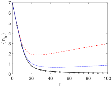
We can further look at how different values of ΓΓ\Gamma can change the effect of cooling. The qualitative trend can be seen clearly from Fig. 3. For a given value of n¯asubscript¯𝑛𝑎\bar{n}_{a}, when ΓΓ\Gamma increases from a small value to a relative large value, there exists a certain ΓΓ\Gamma for which the cooling effect is the largest. Before the optimal cooling point, ΓΓ\Gamma is not large compared with the effective coupling (e.g., gan¯asubscript𝑔𝑎subscript¯𝑛𝑎g_{a}\sqrt{\bar{n}_{a}}), so increase ΓΓ\Gamma will benefit the cooling process. However, after that, larger ΓΓ\Gamma will result in smaller cooling rate. When n¯asubscript¯𝑛𝑎\bar{n}_{a} increases, the optimal ΓΓ\Gamma will increase, too. In the limit of n¯asubscript¯𝑛𝑎\bar{n}_{a}\rightarrow\infty, we can get a simple expression for n^bdelimited-⟨⟩subscript^𝑛𝑏\langle\hat{n}_{b}\rangle under the weak coupling assumption

n^b=12(n¯bγb+Γ2γb+(n¯bγb+Γ2γb)2+2n¯b)delimited-⟨⟩subscript^𝑛𝑏12subscript¯𝑛𝑏subscript𝛾𝑏Γ2subscript𝛾𝑏superscriptsubscript¯𝑛𝑏subscript𝛾𝑏Γ2subscript𝛾𝑏22subscript¯𝑛𝑏\langle\hat{n}_{b}\rangle=\frac{1}{2}\left(\bar{n}_{b}-\frac{\gamma_{b}+\Gamma}{2\gamma_{b}}+\sqrt{(\bar{n}_{b}-\frac{\gamma_{b}+\Gamma}{2\gamma_{b}})^{2}+2\bar{n}_{b}}\right) (12)

As shown in Fig. 3, such an approximation is quite reasonable. In the limit of n¯asubscript¯𝑛𝑎\bar{n}_{a}\rightarrow\infty, the condition for quantum regime cooling (n^b<1delimited-⟨⟩subscript^𝑛𝑏1\langle\hat{n}_{b}\rangle<1) is

Γ>3γb(n¯b1),Γ3subscript𝛾𝑏subscript¯𝑛𝑏1\Gamma>3\gamma_{b}(\bar{n}_{b}-1), (13)

which can be fulfilled by tuning ΓΓ\Gamma with laser. These analytical results are based on rotating wave approximation (RWA). When thermal phonon number n¯aΔ/gabsimilar-tosubscript¯𝑛𝑎Δsubscript𝑔𝑎𝑏\sqrt{\bar{n}_{a}}\sim\Delta/g_{ab}, the RWA is no longer valid. From the parameters used in Fig. 2, RWA requires n¯ab<1012subscript¯𝑛𝑎𝑏superscript1012\bar{n}_{ab}<10^{12}, which is obviously fulfilled in Fig. 2 and the following figures in this paper.
Refer to caption
Figure 3: n^bdelimited-⟨⟩subscript^𝑛𝑏\langle\hat{n}_{b}\rangle as a function of ΓΓ\Gamma. Three values of n¯asubscript¯𝑛𝑎\bar{n}_{a}, 50, 300, 10000, are corresponding to the red dash line, the blue dot line and the black solid line. Black circles display the Eq. (13) in the limit of n¯asubscript¯𝑛𝑎\bar{n}_{a}\rightarrow\infty. The initial temperature of mode b𝑏b is 10.8mK10.8mK10.8\ \rm{mK} so n¯b=7subscript¯𝑛𝑏7\bar{n}_{b}=7. Other parameters are same as Fig. 2.

IV Numerical Simulation

Now we discuss the numerical simulation of the cooling process, and compare the result with the analytical ones above. The idea is simple. We expand the quantum operators and quantum states in the uncoupled representation, that is, the Kronecker tensor product of the occupation number representations for the three modes involved. The matrix forms of Eq. (3) can then be calculated step by step with the classical four-order Runge-Kutta method. The average phonon number for mode b𝑏b is equal to tr(ρNb)tr𝜌subscript𝑁𝑏\mathrm{tr}(\rho N_{b}), where Nbsubscript𝑁𝑏N_{b} is the phonon number operator of mode b𝑏b in the whole Hilbert space for the system, namely, Nb=IsIa(bb)subscript𝑁𝑏tensor-productsubscript𝐼𝑠subscript𝐼𝑎superscript𝑏𝑏N_{b}=I_{s}\otimes I_{a}\otimes(b^{\dagger}b). It should be pointed out, however, as the dimension of a matrix cannot be too large for a numerical simulation, the requirement n¯an¯bmuch-greater-thansubscript¯𝑛𝑎subscript¯𝑛𝑏\bar{n}_{a}\gg\bar{n}_{b} is not able to be satisfied here. As a result, H1subscript𝐻1H_{1} in Eq. (1) should be inserted in the equation of motion Eq. (3) instead of H1superscriptsubscript𝐻1H_{1}^{\prime}.

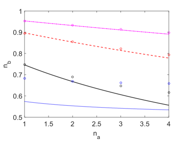
We present several numerical results of the stationary phonon number n^bdelimited-⟨⟩subscript^𝑛𝑏\langle\hat{n}_{b}\rangle with the results we get from Eq. (10), which is plotted in Fig. 4. As can be seen from the figure, when Γγa,γbmuch-greater-thanΓsubscript𝛾𝑎subscript𝛾𝑏\Gamma\gg\gamma_{a},\gamma_{b} is satisfied, the analytical results match the numerical ones perfectly. But when γasubscript𝛾𝑎\gamma_{a} and γbsubscript𝛾𝑏\gamma_{b} is comparable with ΓΓ\Gamma, the two results no longer agree with each other quantitatively. However, it is quite reasonable, because in this case several approximations for the analytical results are not valid any more. When ΓΓ\Gamma is not very large, the term s=ΓDσsubscript𝑠Γsubscript𝐷subscript𝜎\mathcal{L}_{s}=\Gamma D_{\sigma_{-}} does not dominate over H𝐻H in Eq. (3). As n¯asubscript¯𝑛𝑎\bar{n}_{a} is also at the same scale with n¯bsubscript¯𝑛𝑏\bar{n}_{b} in this case, now neglecting the back action on mode a𝑎a is not a good approximation. When mode b𝑏b is being cooled, mode a𝑎a is being heated unavoidably, thus lowering the effect of cooling. The analytical results which neglect the back action thus exaggerate the cooling effect. This trend is shown clearly from the figure. But the analytical conclusions are still valid qualitatively. For instance, if we fix ΓΓ\Gamma, the larger n¯asubscript¯𝑛𝑎\bar{n}_{a} is, the larger the cooling effect will be. And if we fix n¯asubscript¯𝑛𝑎\bar{n}_{a}, there exists a n¯asubscript¯𝑛𝑎\bar{n}_{a}-dependent value of ΓΓ\Gamma where the cooling effect is maximum.

Refer to caption
Figure 4: (color online) Comparison of analytical and numerical results. Lines (circles) represent analytical (numerical) results. We choose four ΓΓ\Gamma: 222 Hz, 151515 Hz, 505050 Hz, 120120120 Hz, corresponding to the blue dot line (blue circles), black solid line (black circles), red dash line (red circles) and pink dash dot line (pink circles). The initial phonon number for mode b𝑏b is taken as n¯b=1subscript¯𝑛𝑏1\bar{n}_{b}=1. Other parameters are same as Fig. 2.

V Discussion and conclusion

From the above derivation and calculation, it is clear the higher frequency mechanical mode will be significantly cooled by heating the lower frequency mechanical mode. In fact, this trend can be seen directly from the Eq. (8), where 1subscript1\mathcal{L}_{1} acts as the cooling term. As the electron spin is much more likely to be in the spin state |0ket0|0\rangle due to the continuous initialization, the effect of σ+subscript𝜎\sigma_{+} should be much larger than that of σsubscript𝜎\sigma_{-}. So Dbσ+subscript𝐷𝑏subscript𝜎D_{b\sigma_{+}} is the dominant operator for evolution, and the mode b𝑏b will be cooled. This can be understood that mode a𝑎a facilitate the energy transfer between mode b𝑏b and the spin. Quantized energy flows from the vibration mode to the NV center. Soon after that the excitation in the NV center electron spin decays into the environment through light. As this process is repeated, the heat of the mechanical mode b𝑏b is gradually removed.

In conclusion, we studied the second order magnetic gradient induced coupling between NV center and the mechanical modes. We proposed to drive one mechanical resonator mode with thermal bath to cool the other mode of the resonator. We solved the motion of the system analytically under the weak coupling assumption. It is found that under rotating wave approximation final thermal phonon number of the resonator approach to a minimum as the thermal bath temperature increases. The quantum regime cooling is feasible under the current experimental conditions. We numerically solved the equations, and found that the results fitted very well with the analytic results. The cooling by heating phenomena does not violate the laws of thermodynamics. This scheme can be understood as a thermal machine or a heat engine Zhang2014 ; Mari2015 ; Mitchison . The mode a𝑎a is an “engine”, and the NV center electron spin takes the role of a “condenser”. This work opens up the possibility that cooling the mechanical mode in solid systems by injecting the thermal phonon, which usually heats the system.

VI Acknowledgements

Z.Q.Y. is supported by National Natural Science Foundation of China Grant 61435007. W.L.Y. is supported by National Natural Science Foundation of China Grant 11574353 and 11274351. P.H and J.D. is supported by 973 Program (Grant No. 2013CB921800), the National Natural Science Foundation of China (Grant No. 11227901), and the CAS (Grant No. XDB01030400).

Appendix A Experimentally realized paramters

In this section we discuss the values of parameters ωzsubscript𝜔𝑧\omega_{z}, ωasubscript𝜔𝑎\omega_{a}, ωbsubscript𝜔𝑏\omega_{b}, gasubscript𝑔𝑎g_{a}, gbsubscript𝑔𝑏g_{b}, gabsubscript𝑔𝑎𝑏g_{ab}, γasubscript𝛾𝑎\gamma_{a}, γbsubscript𝛾𝑏\gamma_{b}, ΓΓ\Gamma that can be realized in experiments.

As in former experiments (e.g. RAB2009 for a Si cantilever), the size of the resonator can be taken as around 3μm×0.05μm×0.05μm3𝜇m0.05𝜇m0.05𝜇m3\rm{\mu m}\times 0.05\rm{\mu m}\times 0.05\rm{\mu m}. Considering that the density of diamond is around 1.5 times the density of silicon Tao2014 , and the fact that the effective mass of a solid and normal shaped oscillator doing simple oscillation is of the same order as its mass, we can estimate that ma=mb=5×10¹⁸subscript𝑚𝑎subscript𝑚𝑏5superscript1018m_{a}=m_{b}=5\times 10^{-18} kg. The fundamental frequency of such a mechanical resonator is around 10 MHz RAB2009 . Although the zero-field splitting of the NV center is around 2.88 GHz Wrachtrup2006 , after an external magnetic field is exerted, the separation between |0ket0|0\rangle and |1ket1|-1\rangle states can be reduced to the order of tens of MHz. As a result, it is possible to fulfill the requirement ωbωa=ωzsubscript𝜔𝑏subscript𝜔𝑎subscript𝜔𝑧\omega_{b}-\omega_{a}=\omega_{z}. Here we choose ωa/2π=10MHzsubscript𝜔𝑎2𝜋10MHz\omega_{a}/2\pi=10\ \rm{MHz}, ωb/2π=30MHzsubscript𝜔𝑏2𝜋30MHz\omega_{b}/2\pi=30\ \rm{MHz} for convenience. The quality factor of the resonator can reach up to Q=107𝑄superscript107Q=10^{7} Tao2014 . Second-order magnetic gradient G2subscript𝐺2G_{2} can realize several times of 1013Tm2superscript1013Tsuperscriptm210^{13}\ \mathrm{T\cdot m^{-2}} in experiment Mamin2007 . By using finite element simulation, we got that the maximum G2subscript𝐺2G_{2} could be around 5×10¹⁴Tm25superscript1014Tsuperscriptm25\times 10^{14}\ \rm{T\cdot m^{-2}}, if the distance between NV center and the magnetic particles is 505050 nm.

If G2subscript𝐺2G_{2} is set to be 5×10¹⁴Tm25superscript1014Tsuperscriptm25\times 10^{14}\ \rm{T\cdot m^{-2}}, we will have ga/2π=3Hzsubscript𝑔𝑎2𝜋3Hzg_{a}/2\pi=3\ \rm{Hz}, gb/2π=1Hzsubscript𝑔𝑏2𝜋1Hzg_{b}/2\pi=1\ \rm{Hz}, gab/2π=1.73Hzsubscript𝑔𝑎𝑏2𝜋1.73Hzg_{ab}/2\pi=1.73\ \rm{Hz}. The decay rates of the mechanical resonator can be estimated by γa=γb=ωa/Q=2π×1Hzsubscript𝛾𝑎subscript𝛾𝑏subscript𝜔𝑎𝑄2𝜋1Hz\gamma_{a}=\gamma_{b}=\omega_{a}/Q=2\pi\times 1\ \rm{Hz}. We need to tune the decay rate of the NV center larger enough than the mechanical decay rate to reach ground state cooling, for instance, ΓΓ\Gamma can equals to 2π×120Hz2𝜋120Hz2\pi\times 120\ \rm{Hz}.

Appendix B Derivation of the Reduced Master Equation

Here we provide a derivation of the reduced master equation Eq. (5) in main text. The reduced density matrix of mode b𝑏b and mode s𝑠s after mode a𝑎a is eliminated is

ρb,s=tra(ρ)subscript𝜌𝑏𝑠subscripttr𝑎𝜌\rho_{b,s}=\mathrm{tr}_{a}(\rho) (14)

We can adiabatically eliminate mode a𝑎a to get the evolution equation for the reduced density matrix QNO

ρ˙b,s(t)=subscript˙𝜌𝑏𝑠𝑡absent\displaystyle\dot{\rho}_{b,s}(t)= i[H0,ρb,s(t)]+bρb,s(t)+sρb,s(t)𝑖subscript𝐻0subscript𝜌𝑏𝑠𝑡subscript𝑏subscript𝜌𝑏𝑠𝑡subscript𝑠subscript𝜌𝑏𝑠𝑡\displaystyle-i[H_{0},\rho_{b,s}(t)]+\mathcal{L}_{b}\rho_{b,s}(t)+\mathcal{L}_{s}\rho_{b,s}(t) (15)
+traint0𝑑tefreetintρb,s(tt)ρasubscripttr𝑎subscript𝑖𝑛𝑡superscriptsubscript0tensor-productdifferential-dsuperscript𝑡superscript𝑒subscript𝑓𝑟𝑒𝑒superscript𝑡subscript𝑖𝑛𝑡subscript𝜌𝑏𝑠𝑡superscript𝑡subscript𝜌𝑎\displaystyle+\mathrm{tr}_{a}\mathcal{L}_{int}\int_{0}^{\infty}dt^{{}^{\prime}}e^{\mathcal{L}_{free}t^{{}^{\prime}}}\mathcal{L}_{int}\rho_{b,s}(t-t^{{}^{\prime}})\otimes\rho_{a}
=\displaystyle= i[H0,ρb,s(t)]+bρb,s(t)+sρb,s(t)𝑖subscript𝐻0subscript𝜌𝑏𝑠𝑡subscript𝑏subscript𝜌𝑏𝑠𝑡subscript𝑠subscript𝜌𝑏𝑠𝑡\displaystyle-i[H_{0},\rho_{b,s}(t)]+\mathcal{L}_{b}\rho_{b,s}(t)+\mathcal{L}_{s}\rho_{b,s}(t)
tra[H1,0𝑑tefreet[H1,ρb,s(tt)ρa]]subscripttr𝑎subscript𝐻1superscriptsubscript0differential-dsuperscript𝑡superscript𝑒subscript𝑓𝑟𝑒𝑒superscript𝑡subscript𝐻1tensor-productsubscript𝜌𝑏𝑠𝑡superscript𝑡subscript𝜌𝑎\displaystyle-\mathrm{tr}_{a}\left[H_{1},\int_{0}^{\infty}dt^{{}^{\prime}}e^{\mathcal{L}_{free}t^{{}^{\prime}}}[H_{1},\rho_{b,s}(t-t^{{}^{\prime}})\otimes\rho_{a}]\right]

where we denote

intsubscript𝑖𝑛𝑡\displaystyle\mathcal{L}_{int} =i[H1,]absent𝑖subscript𝐻1\displaystyle=-i[H_{1},\bullet] (16)
freesubscript𝑓𝑟𝑒𝑒\displaystyle\mathcal{L}_{free} =i[H0,]+a+b+sabsent𝑖subscript𝐻0subscript𝑎subscript𝑏subscript𝑠\displaystyle=-i[H_{0},\bullet]+\mathcal{L}_{a}+\mathcal{L}_{b}+\mathcal{L}_{s}

We expand gasubscript𝑔𝑎g_{a}, gbsubscript𝑔𝑏g_{b} and gabsubscript𝑔𝑎𝑏g_{ab} to the second order and can get

ρ˙b,s(t)=subscript˙𝜌𝑏𝑠𝑡absent\displaystyle\dot{\rho}_{b,s}(t)= i[H0,ρb,s(t)]+bρb,s(t)+sρb,s(t)𝑖subscript𝐻0subscript𝜌𝑏𝑠𝑡subscript𝑏subscript𝜌𝑏𝑠𝑡subscript𝑠subscript𝜌𝑏𝑠𝑡\displaystyle-i[H_{0},\rho_{b,s}(t)]+\mathcal{L}_{b}\rho_{b,s}(t)+\mathcal{L}_{s}\rho_{b,s}(t) (17)
tra[H1,0𝑑t[efreet(H1),ρb,s(t)ρa]]subscripttr𝑎subscript𝐻1superscriptsubscript0differential-dsuperscript𝑡superscript𝑒superscriptsubscript𝑓𝑟𝑒𝑒superscript𝑡subscript𝐻1tensor-productsubscript𝜌𝑏𝑠𝑡subscript𝜌𝑎\displaystyle-\mathrm{tr}_{a}\left[H_{1},\int_{0}^{\infty}dt^{{}^{\prime}}[e^{\mathcal{L}_{free}^{\dagger}t^{{}^{\prime}}}(H_{1}),\rho_{b,s}(t)\otimes\rho_{a}]\right]

Once we expand the commutation relations in Eq. (17), we can directly calculated it term by term.

ρ˙b,s(t)=subscript˙𝜌𝑏𝑠𝑡absent\displaystyle\dot{\rho}_{b,s}(t)= i[H0,ρb,s(t)]+bρb,s(t)+sρb,s(t)𝑖subscript𝐻0subscript𝜌𝑏𝑠𝑡subscript𝑏subscript𝜌𝑏𝑠𝑡subscript𝑠subscript𝜌𝑏𝑠𝑡\displaystyle-i[H_{0},\rho_{b,s}(t)]+\mathcal{L}_{b}\rho_{b,s}(t)+\mathcal{L}_{s}\rho_{b,s}(t) (18)
tra(0dt(H1efreet(H1)ρb,s(t)ρa\displaystyle-\mathrm{tr}_{a}\bigg{(}\int_{0}^{\infty}dt^{{}^{\prime}}\Big{(}H_{1}e^{\mathcal{L}_{free}^{\dagger}t^{{}^{\prime}}}(H_{1})\rho_{b,s}(t)\otimes\rho_{a}
H1ρb,s(t)ρaefreet(H1)tensor-productsubscript𝐻1subscript𝜌𝑏𝑠𝑡subscript𝜌𝑎superscript𝑒superscriptsubscript𝑓𝑟𝑒𝑒superscript𝑡subscript𝐻1\displaystyle-H_{1}\rho_{b,s}(t)\otimes\rho_{a}e^{\mathcal{L}_{free}^{\dagger}t^{{}^{\prime}}}(H_{1})
efreet(H1)ρb,s(t)ρaH1tensor-productsuperscript𝑒superscriptsubscript𝑓𝑟𝑒𝑒superscript𝑡subscript𝐻1subscript𝜌𝑏𝑠𝑡subscript𝜌𝑎subscript𝐻1\displaystyle-e^{\mathcal{L}_{free}^{\dagger}t^{{}^{\prime}}}(H_{1})\rho_{b,s}(t)\otimes\rho_{a}H_{1}
+ρb,s(t)ρaefreet(H1)H1))\displaystyle+\rho_{b,s}(t)\otimes\rho_{a}e^{\mathcal{L}_{free}^{\dagger}t^{{}^{\prime}}}(H_{1})H_{1}\Big{)}\bigg{)}

What we need first is the term efreet(H1)superscript𝑒superscriptsubscript𝑓𝑟𝑒𝑒superscript𝑡subscript𝐻1e^{\mathcal{L}_{free}^{\dagger}t^{{}^{\prime}}}(H_{1}). It is easy to get from direct calculation.

free(a)=superscriptsubscript𝑓𝑟𝑒𝑒𝑎absent\displaystyle\mathcal{L}_{free}^{\dagger}(a)= (1+n¯a)γaDa(a)+n¯aγaDa(a)1subscript¯𝑛𝑎subscript𝛾𝑎superscriptsubscript𝐷𝑎𝑎subscript¯𝑛𝑎subscript𝛾𝑎superscriptsubscript𝐷superscript𝑎𝑎\displaystyle(1+\bar{n}_{a})\gamma_{a}D_{a}^{\dagger}(a)+\bar{n}_{a}\gamma_{a}D_{a^{\dagger}}^{\dagger}(a) (19)
=\displaystyle= (1+n¯a)γa(2aa2aa2aaa)1subscript¯𝑛𝑎subscript𝛾𝑎2superscript𝑎superscript𝑎2superscript𝑎superscript𝑎2𝑎superscript𝑎𝑎\displaystyle(1+\bar{n}_{a})\gamma_{a}(2a^{\dagger}a^{2}-a^{\dagger}a^{2}-aa^{\dagger}a)
+n¯aγa(2a2aaaaa2a)subscript¯𝑛𝑎subscript𝛾𝑎2superscript𝑎2superscript𝑎𝑎superscript𝑎𝑎superscript𝑎2superscript𝑎\displaystyle+\bar{n}_{a}\gamma_{a}(2a^{2}a^{\dagger}-aa^{\dagger}a-a^{2}a^{\dagger})
=\displaystyle= γaasubscript𝛾𝑎𝑎\displaystyle-\gamma_{a}a

Similarly, free(a)=γaasuperscriptsubscript𝑓𝑟𝑒𝑒superscript𝑎subscript𝛾𝑎superscript𝑎\mathcal{L}_{free}^{\dagger}(a^{\dagger})=-\gamma_{a}a^{\dagger}. From these we have efreeta=eγatasuperscript𝑒superscriptsubscript𝑓𝑟𝑒𝑒superscript𝑡𝑎superscript𝑒subscript𝛾𝑎superscript𝑡𝑎e^{\mathcal{L}_{free}^{\dagger}t^{{}^{\prime}}}a=e^{-\gamma_{a}t^{{}^{\prime}}}a, efreeta=eγatasuperscript𝑒superscriptsubscript𝑓𝑟𝑒𝑒superscript𝑡superscript𝑎superscript𝑒subscript𝛾𝑎superscript𝑡superscript𝑎e^{\mathcal{L}_{free}^{\dagger}t^{{}^{\prime}}}a^{\dagger}=e^{-\gamma_{a}t^{{}^{\prime}}}a^{\dagger}.

The following results are got using exactly the same method:

efreetδ=e2γatδ,efreetb=e(γb+iωz)tbformulae-sequencesuperscript𝑒superscriptsubscript𝑓𝑟𝑒𝑒superscript𝑡𝛿superscript𝑒2subscript𝛾𝑎superscript𝑡𝛿superscript𝑒superscriptsubscript𝑓𝑟𝑒𝑒superscript𝑡𝑏superscript𝑒subscript𝛾𝑏𝑖subscript𝜔𝑧superscript𝑡𝑏\displaystyle e^{\mathcal{L}_{free}^{\dagger}t^{{}^{\prime}}}\delta=e^{-2\gamma_{a}t^{{}^{\prime}}}\delta,\ e^{\mathcal{L}_{free}^{\dagger}t^{{}^{\prime}}}b=e^{-(\gamma_{b}+i\omega_{z})t^{{}^{\prime}}}b (20)
efreetb=e(γbiωz)tb,efreetσ+=e(iωzΓ)tσ+formulae-sequencesuperscript𝑒superscriptsubscript𝑓𝑟𝑒𝑒superscript𝑡superscript𝑏superscript𝑒subscript𝛾𝑏𝑖subscript𝜔𝑧superscript𝑡𝑏superscript𝑒superscriptsubscript𝑓𝑟𝑒𝑒superscript𝑡subscript𝜎superscript𝑒𝑖subscript𝜔𝑧Γsuperscript𝑡subscript𝜎\displaystyle e^{\mathcal{L}_{free}^{\dagger}t^{{}^{\prime}}}b^{\dagger}=e^{-(\gamma_{b}-i\omega_{z})t^{{}^{\prime}}}b,\ e^{\mathcal{L}_{free}^{\dagger}t^{{}^{\prime}}}\sigma_{+}=e^{(i\omega_{z}-\Gamma)t^{{}^{\prime}}}\sigma_{+}
efreetσ=e(iωzΓ)tσsuperscript𝑒superscriptsubscript𝑓𝑟𝑒𝑒superscript𝑡subscript𝜎superscript𝑒𝑖subscript𝜔𝑧Γsuperscript𝑡subscript𝜎\displaystyle e^{\mathcal{L}_{free}^{\dagger}t^{{}^{\prime}}}\sigma_{-}=e^{(-i\omega_{z}-\Gamma)t^{{}^{\prime}}}\sigma_{-}

efreet(H1)superscript𝑒superscriptsubscript𝑓𝑟𝑒𝑒superscript𝑡subscript𝐻1e^{\mathcal{L}_{free}^{\dagger}t^{{}^{\prime}}}(H_{1}) will then be calculated with the results above in mind.

efreet(H1)superscript𝑒superscriptsubscript𝑓𝑟𝑒𝑒superscript𝑡subscript𝐻1\displaystyle e^{\mathcal{L}_{free}^{\dagger}t^{{}^{\prime}}}(H_{1}) (21)
=\displaystyle= ga((efreetδ)(efreetσ+)+(efreetδ)(efreetσ))subscript𝑔𝑎superscript𝑒superscriptsubscript𝑓𝑟𝑒𝑒superscript𝑡𝛿superscript𝑒superscriptsubscript𝑓𝑟𝑒𝑒superscript𝑡subscript𝜎superscript𝑒superscriptsubscript𝑓𝑟𝑒𝑒superscript𝑡𝛿superscript𝑒superscriptsubscript𝑓𝑟𝑒𝑒superscript𝑡subscript𝜎\displaystyle g_{a}\Big{(}(e^{\mathcal{L}_{free}^{\dagger}t^{{}^{\prime}}}\delta)(e^{\mathcal{L}_{free}^{\dagger}t^{{}^{\prime}}}\sigma_{+})+(e^{\mathcal{L}_{free}^{\dagger}t^{{}^{\prime}}}\delta)(e^{\mathcal{L}_{free}^{\dagger}t^{{}^{\prime}}}\sigma_{-})\Big{)}
+gab((efreeta)(efreetb)(efreetσ+)\displaystyle+g_{ab}\Big{(}(e^{\mathcal{L}_{free}^{\dagger}t^{{}^{\prime}}}a^{\dagger})(e^{\mathcal{L}_{free}^{\dagger}t^{{}^{\prime}}}b)(e^{\mathcal{L}_{free}^{\dagger}t^{{}^{\prime}}}\sigma_{+})
+(efreeta)(efreetb)(efreetσ))\displaystyle+(e^{\mathcal{L}_{free}^{\dagger}t^{{}^{\prime}}}a)(e^{\mathcal{L}_{free}^{\dagger}t^{{}^{\prime}}}b^{\dagger})(e^{\mathcal{L}_{free}^{\dagger}t^{{}^{\prime}}}\sigma_{-})\Big{)}
=\displaystyle= gaδe(2γa+Γ)t(σ+eiωzt+σeiωzt)subscript𝑔𝑎𝛿superscript𝑒2subscript𝛾𝑎Γsuperscript𝑡subscript𝜎superscript𝑒𝑖subscript𝜔𝑧superscript𝑡subscript𝜎superscript𝑒𝑖subscript𝜔𝑧superscript𝑡\displaystyle g_{a}\delta e^{-(2\gamma_{a}+\Gamma)t^{{}^{\prime}}}(\sigma_{+}e^{i\omega_{z}t^{{}^{\prime}}}+\sigma_{-}e^{-i\omega_{z}t^{{}^{\prime}}})
+gabe(γa+γb+Γ)t(abσ++abσ)subscript𝑔𝑎𝑏superscript𝑒subscript𝛾𝑎subscript𝛾𝑏Γsuperscript𝑡superscript𝑎𝑏subscript𝜎𝑎superscript𝑏subscript𝜎\displaystyle+g_{ab}e^{-(\gamma_{a}+\gamma_{b}+\Gamma)t^{{}^{\prime}}}(a^{\dagger}b\sigma_{+}+ab^{\dagger}\sigma_{-})

It deserves notice that here we only keep the slow-time-varying term, so we neglect a2superscript𝑎absent2a^{\dagger 2} and a2superscript𝑎2a^{2} above. Now we come back to Eq. (18), which can be simplified term by term. As trasubscripttr𝑎\mathrm{tr}_{a} means taking the average on a𝑎a, the trace of odd multiples of a𝑎a and asuperscript𝑎a^{\dagger} equals to zero. Terms containing iωz𝑖subscript𝜔𝑧i\omega_{z} are neglected here because their effect is just changing the energy zero point.

tra(0𝑑tH1efreet(H1)ρb,s(t)ρa)subscripttr𝑎superscriptsubscript0tensor-productdifferential-dsuperscript𝑡subscript𝐻1superscript𝑒superscriptsubscript𝑓𝑟𝑒𝑒superscript𝑡subscript𝐻1subscript𝜌𝑏𝑠𝑡subscript𝜌𝑎\displaystyle\mathrm{tr}_{a}\Big{(}\int_{0}^{\infty}dt^{{}^{\prime}}H_{1}e^{\mathcal{L}_{free}^{\dagger}t^{{}^{\prime}}}(H_{1})\rho_{b,s}(t)\otimes\rho_{a}\Big{)} (22)
=\displaystyle= ga2(n¯a2+n¯a)2γa+Γωz2+(2γa+Γ)2(σ+σ+σσ+)ρb,s(t)superscriptsubscript𝑔𝑎2superscriptsubscript¯𝑛𝑎2subscript¯𝑛𝑎2subscript𝛾𝑎Γsuperscriptsubscript𝜔𝑧2superscript2subscript𝛾𝑎Γ2subscript𝜎subscript𝜎subscript𝜎subscript𝜎subscript𝜌𝑏𝑠𝑡\displaystyle g_{a}^{2}(\bar{n}_{a}^{2}+\bar{n}_{a})\frac{2\gamma_{a}+\Gamma}{\omega_{z}^{2}+(2\gamma_{a}+\Gamma)^{2}}(\sigma_{+}\sigma_{-}+\sigma_{-}\sigma_{+})\rho_{b,s}(t)
+gab2γa+γb+Γ((n¯a+1)bσbσ++n¯abσ+bσ)ρb,s(t)superscriptsubscript𝑔𝑎𝑏2subscript𝛾𝑎subscript𝛾𝑏Γsubscript¯𝑛𝑎1superscript𝑏subscript𝜎𝑏subscript𝜎subscript¯𝑛𝑎𝑏subscript𝜎superscript𝑏subscript𝜎subscript𝜌𝑏𝑠𝑡\displaystyle+\frac{g_{ab}^{2}}{\gamma_{a}+\gamma_{b}+\Gamma}\Big{(}(\bar{n}_{a}+1)b^{\dagger}\sigma_{-}b\sigma_{+}+\bar{n}_{a}b\sigma_{+}b^{\dagger}\sigma_{-}\Big{)}\rho_{b,s}(t)
tra(0𝑑tH1ρb,s(t)ρaefreet(H1))subscripttr𝑎superscriptsubscript0tensor-productdifferential-dsuperscript𝑡subscript𝐻1subscript𝜌𝑏𝑠𝑡subscript𝜌𝑎superscript𝑒superscriptsubscript𝑓𝑟𝑒𝑒superscript𝑡subscript𝐻1\displaystyle\mathrm{tr}_{a}\Big{(}\int_{0}^{\infty}dt^{{}^{\prime}}H_{1}\rho_{b,s}(t)\otimes\rho_{a}e^{\mathcal{L}_{free}^{\dagger}t^{{}^{\prime}}}(H_{1})\Big{)} (23)
=\displaystyle= ga2(n¯a2+n¯a)2γa+Γωz2+(2γa+Γ)2(σ+ρb,s(t)σ+σρb,s(t)σ+)superscriptsubscript𝑔𝑎2superscriptsubscript¯𝑛𝑎2subscript¯𝑛𝑎2subscript𝛾𝑎Γsuperscriptsubscript𝜔𝑧2superscript2subscript𝛾𝑎Γ2subscript𝜎subscript𝜌𝑏𝑠𝑡subscript𝜎subscript𝜎subscript𝜌𝑏𝑠𝑡subscript𝜎\displaystyle g_{a}^{2}(\bar{n}_{a}^{2}+\bar{n}_{a})\frac{2\gamma_{a}+\Gamma}{\omega_{z}^{2}+(2\gamma_{a}+\Gamma)^{2}}(\sigma_{+}\rho_{b,s}(t)\sigma_{-}+\sigma_{-}\rho_{b,s}(t)\sigma_{+})
+gab2γa+γb+Γ((n¯a+1)bσ+ρb,s(t)bσ+n¯abσρb,s(t)bσ+)superscriptsubscript𝑔𝑎𝑏2subscript𝛾𝑎subscript𝛾𝑏Γsubscript¯𝑛𝑎1𝑏subscript𝜎subscript𝜌𝑏𝑠𝑡superscript𝑏subscript𝜎subscript¯𝑛𝑎superscript𝑏subscript𝜎subscript𝜌𝑏𝑠𝑡𝑏subscript𝜎\displaystyle+\frac{g_{ab}^{2}}{\gamma_{a}+\gamma_{b}+\Gamma}\Big{(}(\bar{n}_{a}+1)b\sigma_{+}\rho_{b,s}(t)b^{\dagger}\sigma_{-}+\bar{n}_{a}b^{\dagger}\sigma_{-}\rho_{b,s}(t)b\sigma_{+}\Big{)}
tra(0𝑑tefreet(H1)ρb,s(t)ρaH1)subscripttr𝑎superscriptsubscript0tensor-productdifferential-dsuperscript𝑡superscript𝑒superscriptsubscript𝑓𝑟𝑒𝑒superscript𝑡subscript𝐻1subscript𝜌𝑏𝑠𝑡subscript𝜌𝑎subscript𝐻1\displaystyle\mathrm{tr}_{a}\Big{(}\int_{0}^{\infty}dt^{{}^{\prime}}e^{\mathcal{L}_{free}^{\dagger}t^{{}^{\prime}}}(H_{1})\rho_{b,s}(t)\otimes\rho_{a}H_{1}\Big{)} (24)
=\displaystyle= ga2(n¯a2+n¯a)2γa+Γωz2+(2γa+Γ)2(σ+ρb,s(t)σ+σρb,s(t)σ+)superscriptsubscript𝑔𝑎2superscriptsubscript¯𝑛𝑎2subscript¯𝑛𝑎2subscript𝛾𝑎Γsuperscriptsubscript𝜔𝑧2superscript2subscript𝛾𝑎Γ2subscript𝜎subscript𝜌𝑏𝑠𝑡subscript𝜎subscript𝜎subscript𝜌𝑏𝑠𝑡subscript𝜎\displaystyle g_{a}^{2}(\bar{n}_{a}^{2}+\bar{n}_{a})\frac{2\gamma_{a}+\Gamma}{\omega_{z}^{2}+(2\gamma_{a}+\Gamma)^{2}}(\sigma_{+}\rho_{b,s}(t)\sigma_{-}+\sigma_{-}\rho_{b,s}(t)\sigma_{+})
+gab2γa+γb+Γ((n¯a+1)bσ+ρb,s(t)bσ+n¯abσρb,s(t)bσ+)superscriptsubscript𝑔𝑎𝑏2subscript𝛾𝑎subscript𝛾𝑏Γsubscript¯𝑛𝑎1𝑏subscript𝜎subscript𝜌𝑏𝑠𝑡superscript𝑏subscript𝜎subscript¯𝑛𝑎superscript𝑏subscript𝜎subscript𝜌𝑏𝑠𝑡𝑏subscript𝜎\displaystyle+\frac{g_{ab}^{2}}{\gamma_{a}+\gamma_{b}+\Gamma}\Big{(}(\bar{n}_{a}+1)b\sigma_{+}\rho_{b,s}(t)b^{\dagger}\sigma_{-}+\bar{n}_{a}b^{\dagger}\sigma_{-}\rho_{b,s}(t)b\sigma_{+}\Big{)}
tra(0𝑑tρb,s(t)ρaefreet(H1)H1)subscripttr𝑎superscriptsubscript0tensor-productdifferential-dsuperscript𝑡subscript𝜌𝑏𝑠𝑡subscript𝜌𝑎superscript𝑒superscriptsubscript𝑓𝑟𝑒𝑒superscript𝑡subscript𝐻1subscript𝐻1\displaystyle\mathrm{tr}_{a}\Big{(}\int_{0}^{\infty}dt^{{}^{\prime}}\rho_{b,s}(t)\otimes\rho_{a}e^{\mathcal{L}_{free}^{\dagger}t^{{}^{\prime}}}(H_{1})H_{1}\Big{)} (25)
=\displaystyle= ga2(n¯a2+n¯a)2γa+Γωz2+(2γa+Γ)2ρb,s(t)(σ+σ+σσ+)superscriptsubscript𝑔𝑎2superscriptsubscript¯𝑛𝑎2subscript¯𝑛𝑎2subscript𝛾𝑎Γsuperscriptsubscript𝜔𝑧2superscript2subscript𝛾𝑎Γ2subscript𝜌𝑏𝑠𝑡subscript𝜎subscript𝜎subscript𝜎subscript𝜎\displaystyle g_{a}^{2}(\bar{n}_{a}^{2}+\bar{n}_{a})\frac{2\gamma_{a}+\Gamma}{\omega_{z}^{2}+(2\gamma_{a}+\Gamma)^{2}}\rho_{b,s}(t)(\sigma_{+}\sigma_{-}+\sigma_{-}\sigma_{+})
+gab2γa+γb+Γρb,s(t)((n¯a+1)bσbσ++n¯abσ+bσ)superscriptsubscript𝑔𝑎𝑏2subscript𝛾𝑎subscript𝛾𝑏Γsubscript𝜌𝑏𝑠𝑡subscript¯𝑛𝑎1superscript𝑏subscript𝜎𝑏subscript𝜎subscript¯𝑛𝑎𝑏subscript𝜎superscript𝑏subscript𝜎\displaystyle+\frac{g_{ab}^{2}}{\gamma_{a}+\gamma_{b}+\Gamma}\rho_{b,s}(t)\Big{(}(\bar{n}_{a}+1)b^{\dagger}\sigma_{-}b\sigma_{+}+\bar{n}_{a}b\sigma_{+}b^{\dagger}\sigma_{-}\Big{)}

After we insert Eq. (22), (23), (24), (25) into Eq. (18), we will get Eq. (5) in the main text.

Appendix C Derivation of the Adjoint Equations for the Number Operators

In this part, the equations of motion for the number operators n^bsubscript^𝑛𝑏\hat{n}_{b} and n^ssubscript^𝑛𝑠\hat{n}_{s}, Eq. (9) in main text, is derived.

The adjoint equations for Eq. (9) in main text are

ddtn^s=𝑑𝑑𝑡subscript^𝑛𝑠absent\displaystyle\frac{d}{dt}\hat{n}_{s}= (1+s)n^s\displaystyle(\mathcal{L}_{1}^{\dagger}+\mathcal{L}_{s}^{{}^{\prime}\dagger})\hat{n}_{s} (26)
=\displaystyle= gab2γa+γb+Γ((1+n¯a)Dbσ++n¯aDbσ)n^ssuperscriptsubscript𝑔𝑎𝑏2subscript𝛾𝑎subscript𝛾𝑏Γ1subscript¯𝑛𝑎superscriptsubscript𝐷𝑏subscript𝜎subscript¯𝑛𝑎superscriptsubscript𝐷superscript𝑏subscript𝜎subscript^𝑛𝑠\displaystyle\frac{g_{ab}^{2}}{\gamma_{a}+\gamma_{b}+\Gamma}\left((1+\bar{n}_{a})D_{b\sigma_{+}}^{\dagger}+\bar{n}_{a}D_{b^{\dagger}\sigma_{-}}^{\dagger}\right)\hat{n}_{s}
+((1+ns)ΓDσ+nsΓDσ+)n^s1superscriptsubscript𝑛𝑠Γsuperscriptsubscript𝐷subscript𝜎superscriptsubscript𝑛𝑠Γsuperscriptsubscript𝐷subscript𝜎subscript^𝑛𝑠\displaystyle+\left((1+n_{s}^{{}^{\prime}})\Gamma D_{\sigma_{-}}^{\dagger}+n_{s}^{{}^{\prime}}\Gamma D_{\sigma_{+}}^{\dagger}\right)\hat{n}_{s}
ddtn^b=𝑑𝑑𝑡subscript^𝑛𝑏absent\displaystyle\frac{d}{dt}\hat{n}_{b}= (1+b)n^bsuperscriptsubscript1superscriptsubscript𝑏subscript^𝑛𝑏\displaystyle(\mathcal{L}_{1}^{\dagger}+\mathcal{L}_{b}^{\dagger})\hat{n}_{b}
=\displaystyle= gab2γa+γb+Γ((1+n¯a)Dbσ++n¯aDbσ)n^bsuperscriptsubscript𝑔𝑎𝑏2subscript𝛾𝑎subscript𝛾𝑏Γ1subscript¯𝑛𝑎superscriptsubscript𝐷𝑏subscript𝜎subscript¯𝑛𝑎superscriptsubscript𝐷superscript𝑏subscript𝜎subscript^𝑛𝑏\displaystyle\frac{g_{ab}^{2}}{\gamma_{a}+\gamma_{b}+\Gamma}\left((1+\bar{n}_{a})D_{b\sigma_{+}}^{\dagger}+\bar{n}_{a}D_{b^{\dagger}\sigma_{-}}^{\dagger}\right)\hat{n}_{b}
+((1+n¯b)γbDb+n¯bγbDb)n^b1subscript¯𝑛𝑏subscript𝛾𝑏superscriptsubscript𝐷𝑏subscript¯𝑛𝑏subscript𝛾𝑏superscriptsubscript𝐷superscript𝑏subscript^𝑛𝑏\displaystyle+\left((1+\bar{n}_{b})\gamma_{b}D_{b}^{\dagger}+\bar{n}_{b}\gamma_{b}D_{b^{\dagger}}^{\dagger}\right)\hat{n}_{b}

From simple calculations, we have

Dbσ+(n^s)=2(1n^s)n^b,Dbσ(n^s)=2n^s(1+n^b)formulae-sequencesuperscriptsubscript𝐷𝑏subscript𝜎subscript^𝑛𝑠21subscript^𝑛𝑠subscript^𝑛𝑏superscriptsubscript𝐷superscript𝑏subscript𝜎subscript^𝑛𝑠2subscript^𝑛𝑠1subscript^𝑛𝑏\displaystyle D_{b\sigma_{+}}^{\dagger}(\hat{n}_{s})=2(1-\hat{n}_{s})\hat{n}_{b},\ D_{b^{\dagger}\sigma_{-}}^{\dagger}(\hat{n}_{s})=-2\hat{n}_{s}(1+\hat{n}_{b}) (27)
Dσ+(n^s)=2(1n^s),Dσ(n^s)=2n^sformulae-sequencesuperscriptsubscript𝐷subscript𝜎subscript^𝑛𝑠21subscript^𝑛𝑠superscriptsubscript𝐷subscript𝜎subscript^𝑛𝑠2subscript^𝑛𝑠\displaystyle D_{\sigma_{+}}^{\dagger}(\hat{n}_{s})=2(1-\hat{n}_{s}),\ D_{\sigma_{-}}^{\dagger}(\hat{n}_{s})=-2\hat{n}_{s}
Dbσ+(n^b)=2(1n^s)n^b,Dbσ(n^b)=2n^s(1+n^b)formulae-sequencesuperscriptsubscript𝐷𝑏subscript𝜎subscript^𝑛𝑏21subscript^𝑛𝑠subscript^𝑛𝑏superscriptsubscript𝐷superscript𝑏subscript𝜎subscript^𝑛𝑏2subscript^𝑛𝑠1subscript^𝑛𝑏\displaystyle D_{b\sigma_{+}}^{\dagger}(\hat{n}_{b})=-2(1-\hat{n}_{s})\hat{n}_{b},\ D_{b^{\dagger}\sigma_{-}}^{\dagger}(\hat{n}_{b})=2\hat{n}_{s}(1+\hat{n}_{b})
Db(n^b)=2n^b,Db(n^b)=2(1+n^b)formulae-sequencesuperscriptsubscript𝐷𝑏subscript^𝑛𝑏2subscript^𝑛𝑏superscriptsubscript𝐷superscript𝑏subscript^𝑛𝑏21subscript^𝑛𝑏\displaystyle D_{b}^{\dagger}(\hat{n}_{b})=-2\hat{n}_{b},\ D_{b^{\dagger}}^{\dagger}(\hat{n}_{b})=2(1+\hat{n}_{b})

After Eq. (27) is inserted into Eq. (26), it will be simplified to Eq. (9) in the main text.

Appendix D Detail of the Numerical Simulation

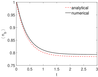
In this section, we discuss in detail the numerical simulation. For Fig. 4 in main text, we control the accuracy so that all numbers are accurate until the order of 0.001. The evolution time is t=3𝑡3t=3, after which the state is at the stationary state up to the accuracy. As discussed in the Appendix before, we can renormalize the frequency parameters as gab=3subscript𝑔𝑎𝑏3g_{ab}=\sqrt{3}, gb=1subscript𝑔𝑏1g_{b}=1, ga=3subscript𝑔𝑎3g_{a}=3, γa=γb=1subscript𝛾𝑎subscript𝛾𝑏1\gamma_{a}=\gamma_{b}=1. As we want to cover a wide range of results, four values renormalized ΓΓ\Gamma are chosen: 2, 15, 50 and 120. Small values for the phonon numbers n¯asubscript¯𝑛𝑎\bar{n}_{a} and n¯bsubscript¯𝑛𝑏\bar{n}_{b} should be chosen due to the calculation cost.
Refer to caption
Figure 5: The time evolution of the phonon number of mode b𝑏b. Here Γ=50Γ50\Gamma=50. Initial phonon numbers are: n¯a=4subscript¯𝑛𝑎4\bar{n}_{a}=4, n¯b=1subscript¯𝑛𝑏1\bar{n}_{b}=1. The matrix dimension of the operators and states for mode a𝑎a is taken to be 60×60606060\times 60, for mode b𝑏b it is 15×15151515\times 15. Other parameters are same as Fig. 2 in main text. For the analytical solution of the differential equation Eq. (9) in main text, standard solver ode45 in Matlab is used.

Here we always choose n¯b=1subscript¯𝑛𝑏1\bar{n}_{b}=1 as the initial condition. As to n¯asubscript¯𝑛𝑎\bar{n}_{a}, we choose n¯a=1,2,3,4subscript¯𝑛𝑎1234\bar{n}_{a}=1,2,3,4. The dimensions of the matrices in the Hilbert space are chosen to balance the accuracy and the cost of calculation resource. For the Hilbert space where the initial phonon number equals to 1, the dimension is chosen as 15×15151515\times 15. For the Hilbert space where the initial phonon number equals to 2, the dimension is chosen as 27×27272727\times 27. For the Hilbert space where the initial phonon number equals to 3, the dimension is chosen as 40×40404040\times 40. For the Hilbert space where the initial phonon number equals to 4, the dimension is chosen as 60×60606060\times 60. Obviously, the dimension of the Hilbert space for mode s𝑠s is always 2×2222\times 2. The step length for the Runge-Kutta method is chosen to be 0.01/500.01500.01/50.

Fig. 4 in the main text shows the results of only the ωz=500subscript𝜔𝑧500\omega_{z}=500 case, even if for the example in the Appendix, ωzsubscript𝜔𝑧\omega_{z} should be renormalized as ωz=2×10⁷subscript𝜔𝑧2superscript107\omega_{z}=2\times 10^{7}. In fact, we have tried that different ωzsubscript𝜔𝑧\omega_{z} will not influence the result of cooling, e.g., ωz=250, 500, 750subscript𝜔𝑧250500750\omega_{z}=250,\ 500,\ 750 all give out same final phonon number for mode b𝑏b. So we are safe to use smaller ωzsubscript𝜔𝑧\omega_{z} here considering the stability of the simulation. This deduction also agrees with the analytical result because Eq. (10) in main text does not contain ωzsubscript𝜔𝑧\omega_{z} as long as ωzsubscript𝜔𝑧\omega_{z} is large enough for ns0superscriptsubscript𝑛𝑠0n_{s}^{{}^{\prime}}\approx 0.

The time evolution of one set of parameters from numerical simulation is shown in Fig. 5. The phonon occupation number n^bdelimited-⟨⟩subscript^𝑛𝑏\langle\hat{n}_{b}\rangle gradually goes down as the system evolves towards the stationary state. The cooling effect indeed happens. Also shown in the figure is the time evolution starting from the analytical result Eq. (9). The two lines are similar with the cooling effect of the analytical one a little bit more obvious, which also supports our findings.

References

  • (1) M. Aspelmeyer, T. J. Kippenberg, and F. Marquardt, Reviews of Modern Physics 86, 1391 (2014).
  • (2) C. Regal and K. Lehnert, in Journal of Physics: Conference Series (IOP Publishing, 2011), p. 012025.
  • (3) S. Barzanjeh, M. Abdi, G. J. Milburn, P. Tombesi, and D. Vitali, Phys. Rev. Lett. 109, 130503 (2012).
  • (4) Y. Wang and A. A. Clerk, Phys. Rev. Lett. 108, 153603 (2012).
  • (5) L. Tian, Phys. Rev. Lett. 108, 153604 (2012).
  • (6) S. Rips and M. J. Hartmann, Phys. Rev. Lett. 110, 120503 (2013).
  • (7) Z. Yin and Y. Han, Physical Review A 79, 024301 (2009).
  • (8) Z. Yin, W. Yang, L. Sun, and L. Duan, Physical Review A 91, 012333 (2015).
  • (9) S. Barzanjeh, S. Guha, C. Weedbrook, D. Vitali, J. H. Shapiro, and S. Pirandola, Phys. Rev. Lett. 114, 080503 (2015).
  • (10) R. Penrose, General relativity and gravitation 28, 581 (1996).
  • (11) A. D. O’Connell, M. Hofheinz, M. Ansmann, R. C. Bialczak, M. Lenander, E. Lucero, M. Neeley, D. Sank, H. Wang, and M. Weides, Nature 464, 697 (2010).
  • (12) J. Teufel, T. Donner, D. Li, J. Harlow, M. Allman, K. Cicak, A. Sirois, J. D. Whittaker, K. Lehnert, and R. W. Simmonds, Nature 475, 359 (2011).
  • (13) M. Poot and van der Zant, Herre SJ, Physics Reports 511, 273 (2012).
  • (14) I. Pikovski, M. R. Vanner, M. Aspelmeyer, M. Kim, and C̆. Brukner, Nature Physics 8, 393 (2012).
  • (15) S. Nimmrichter and K. Hornberger, Phys. Rev. Lett. 110, 160403 (2013).
  • (16) A. Bassi, K. Lochan, S. Satin, T. P. Singh, and H. Ulbricht, Reviews of Modern Physics 85, 471 (2013).
  • (17) O. Romero-Isart, A. C. Pflanzer, F. Blaser, R. Kaltenbaek, N. Kiesel, M. Aspelmeyer, and J. I. Cirac, Phys. Rev. Lett. 107, 020405 (2011).
  • (18) Z. Yin, T. Li, X. Zhang, and L. Duan, Physical Review A 88, 033614 (2013).
  • (19) T. Li and Z. Yin, Science Bulletin 61, 163 (2016).
  • (20) S. Barzanjeh and D. Vitali, Physical Review A 93, 033846 (2016).
  • (21) C. M. Caves, Physical Review D 23, 1693 (1981).
  • (22) A. A. Geraci, S. B. Papp, and J. Kitching, Phys. Rev. Lett. 105, 101101 (2010).
  • (23) Z. Yin, T. Li, and M. Feng, Physical Review A 83, 013816 (2011).
  • (24) A. Arvanitaki and A. A. Geraci, Phys. Rev. Lett. 110, 071105 (2013).
  • (25) P. Huang, P. Wang, J. Zhou, Z. Wang, C. Ju, Z. Wang, Y. Shen, C. Duan, and J. Du, Phys. Rev. Lett. 110, 227202 (2013).
  • (26) N. Zhao and Z. Yin, Physical Review A 90, 042118 (2014).
  • (27) I. Wilson-Rae, N. Nooshi, W. Zwerger, and T. J. Kippenberg, Phys. Rev. Lett. 99, 093901 (2007).
  • (28) F. Marquardt, J. P. Chen, A. Clerk, and S. Girvin, Phys. Rev. Lett. 99, 093902 (2007).
  • (29) Liu Yong-Chun, Hu Yu-Wen, Wong Chee We, and Xiao Yun-Feng, Chinese Physics B 22, 114213 (2013).
  • (30) P. Rabl, P. Cappellaro, M. G. Dutt, L. Jiang, J. Maze, and M. D. Lukin, Physical Review B 79, 041302 (2009).
  • (31) E. MacQuarrie, M. Otten, S. Gray, and G. Fuchs, arXiv preprint arXiv:1605.07131 (2016).
  • (32) P. Li, Z. Xiang, P. Rabl, and F. Nori, Phys. Rev. Lett. 117, 015502 (2016).
  • (33) A. Mari and J. Eisert, Phys. Rev. Lett. 108, 120602 (2012).
  • (34) Z. Yin, Physical Review A 80, 033821 (2009).
  • (35) L. Zhou, L. Wei, M. Gao, and X. Wang, Physical Review A 81, 042323 (2010).
  • (36) Z. Xu, Y. Hu, W. Yang, M. Feng, and J. Du, Physical Review A 80, 022335 (2009).
  • (37) Q. Chen, Z. Xu, and M. Feng, Physical Review A 82, 014302 (2010).
  • (38) O. Arcizet, V. Jacques, A. Siria, P. Poncharal, P. Vincent, and S. Seidelin, Nature Physics 7, 879 (2011).
  • (39) S. Kolkowitz, A. C. Jayich, Q. P. Unterreithmeier, S. D. Bennett, P. Rabl, J. G. Harris, and M. D. Lukin, Science 335, 1603 (2012).
  • (40) Z. Yin, N. Zhao, and T. Li, Science China Physics, Mechanics & Astronomy 58, 1 (2015).
  • (41) J. Cai, B. Naydenov, R. Pfeiffer, L. P. McGuinness, K. D. Jahnke, F. Jelezko, M. B. Plenio, and A. Retzker, New Journal of Physics 14, 113023 (2012).
  • (42) H. Breuer and F. Petruccione, The theory of open quantum systems (Oxford University Press on Demand, 2002).
  • (43) C. Gardiner and P. Zoller, Quantum noise: a handbook of Markovian and non-Markovian quantum stochastic methods with applications to quantum optics (Springer Science & Business Media, 2004), 56.
  • (44) Z. Yin, F. Li, and P. Peng, Physical Review A 76, 062311 (2007).
  • (45) C. Yang, J. An, W. Yang, and Y. Li, Physical Review A 92, 062311 (2015).
  • (46) J. Wrachtrup and F. Jelezko, Journal of Physics: Condensed Matter 18, S807 (2006).
  • (47) Y. Tao, J. Boss, B. Moores, and C. Degen, Nature communications 5 (2014).
  • (48) H. Mamin, M. Poggio, C. Degen, and D. Rugar, Nature nanotechnology 2, 301 (2007).
  • (49) K. Zhang, F. Bariani, and P. Meystre, Phys. Rev. Lett. 112, 150602 (2014).
  • (50) A. Mari, A. Farace, and V. Giovannetti, Journal of Physics B: Atomic, Molecular and Optical Physics 48, 175501 (2015).
  • (51) M. T. Mitchison, M. Huber, J. Prior, M. P. Woods, and M. B. Plenio, arXiv preprint arXiv:1603.02082 (2016).