Modeling, dynamics and optimal control
of Ebola virus spread

Abstract.

We present a mathematical analysis of the early detection of Ebola virus. The propagation of the virus is analysed by using a Susceptible, Infected, Recovered (SIR) model. In order to provide useful predictions about the potential transmission of the virus, we analyse and simulate the SIR model with vital dynamics, by adding demographic effects and an induced death rate. Then, we compute the equilibria of the model. The numerical simulations confirm the theoretical analysis. Our study describes the 2015 detection of Ebola virus in Guinea, the parameters of the model being identified from the World Health Organization data. Finally, we consider an optimal control problem of the propagation of the Ebola virus, minimizing the number of infected individuals while taking into account the cost of vaccination.

1. Introduction

Ebola virus is currently affecting several African countries, mainly Guinea, Sierra Leone, and Liberia. Ebola was first discovered in 1976 in the Democratic Republic of the Congo near the Ebola River, where the disease takes its name [5, 10, 19]. Since then, Ebola outbreaks have appeared sporadically in Africa. The virus, previously known as Ebola haemorrhagic fever, is the deadliest pathogens for humans. The early signs and symptoms of the virus include a sudden onset of fever and intense weakness and headache. Over time, symptoms become increasingly severe and include diarrhoea, raised rash, internal and external bleed in (from nose, mouth, eyes and anus). As the virus spreads through the body, it damages the immune system and organs [18, 26, 29, 32, 34]. Ebola virus is transmitted to an initial human by contact with an infected animal’s body fluid. On the other hand, human-to-human transmission can take place with direct contact (through broken skin or mucous membranes in, for example, the eyes, nose, or mouth) with blood or body fluids of a person who is sick with or has died from Ebola. It is also transmitted indirectly via exposure to objects or environment contaminated with infected secretions [1, 8, 12, 21, 30].

Mathematical models are a powerful tool for investigating human infectious diseases, such as Ebola, contributing to the understanding of the dynamics of the disease, providing useful predictions about the potential transmission of the disease and the effectiveness of possible control measures, which can provide valuable information for public health policy makers [11, 14, 27, 28]. Epidemic models date back to the early twentieth century, to the 1927 work by Kermack and McKendrick, whose model was used for modelling the plague and cholera epidemics. In fact, such epidemic models have provided the foundation for the best vaccination practices for influenza [20] and small pox [17]. Currently, the simplest and most commonly implemented model in epidemiology is the SIR model. The SIR model consists of three compartments: Susceptible individuals $S$, Infectious individuals $I$, and Recovered individuals $R$ [15]. When analysing a new outbreak, the researchers usually start with the SIR model to fit the available outbreak data and obtaining estimates for the parameters of the model [9]. This has been the case for the modelling of the spreading mechanism of the Ebola virus currently affecting several African countries [22, 23, 25]. For more complex mathematical models, with more than three state variables, see [2, 3, 24].

In our previous works [22, 25], we used parameters identified from the recent data of the World Health Organization (WHO) to describe the behaviour of the virus. Here we focus on the mathematical analysis of the early detection of the Ebola virus. In Section 2, we briefly recall the analysis study of the SIR model that we presented in our previous study of the description of the behaviour of Ebola virus [22, 23]. In Section 3, we add to the basic model of Section 2 the demographic effects, in order to provide a description of the virus propagation closer to the reality. This gives answer to an open question posed in Remark 1 of [24] and at the end of [3]. Our aim in studying the model with vital dynamics is to provide useful predictions about the potential transmission of the virus. We also consider an induced death rate for the infected individuals. After numerical simulations, in Section 4 we control the propagation of the virus in order to minimize the number of infected individuals and the cost of vaccination. We end with Section 5 of conclusions.

2. Mathematical formulation for the basic SIR model

In this section, we present and briefly discuss the properties of the system of equations corresponding to the basic SIR (Susceptible–Infectious–Recovery) model, which has recently been used in [22] to describe the early detection of Ebola virus in West Africa. In the formulation of the basic SIR model, we assume that the population size is constant and any person who has completely recovered from the virus acquired permanent immunity. Moreover, we assume that the virus has a negligibly short incubation period, so that an individual who contracts the virus becomes infective immediately afterwards. These assumptions enables us to divide the host population into three categories,

• $S(t)$ for susceptible: denotes individuals who are susceptible to catch the virus, and so might become infectious if exposed;

• $I(t)$ for Infectious: denotes infectious individuals who are able to spread the virus through contact with the susceptible category;

• $R(t)$ for Recovered: denotes individuals who have immunity to the infection, and consequently do not affect the transmission dynamics in any way when in contact with other individuals.

The model is described mathematically by the following system of non-linear differential equations:

(2.1) $$\begin{cases}\dfrac{dS(t)}{dt}=-\beta S(t)I(t),\\[5.69046pt] \dfrac{dI(t)}{dt}=\beta S(t)I(t)-\mu I(t),\\[5.69046pt] \dfrac{dR(t)}{dt}=\mu I(t),\end{cases}$$

where $\beta>0$ is the infection rate and $\mu>0$ is the recovered rate. The initial conditions are given by

(2.2) $$S(0)=S_{0}>0,\quad I(0)=I_{0}>0,\quad R(0)=0.$$

We can see that $\dfrac{d}{dt}\left[S(t)+I(t)+R(t)\right]=0$, that is, the population size $N$ is constant during the period under study:

(2.3) $$S(t)+I(t)+R(t)=N$$

for any $t\geq 0$, which is far from the reality.

3. SIR model with vital dynamics and an induced death rate

In the basic SIR model (2.1), we ignore the demographic effects on the population. In this section, we study a variant of the basic model by considering vital dynamics, that is, by adding the birth and death rates into the model. Moreover, we increase the death rate of the infectious class by considering an induced death rate associated to the infected individuals. Such model is new in the Ebola context [22, 25, 33].

3.1. Model formulation

If we expand the SIR model (2.1) by including the demographic effects, assuming a constant rate of births $\psi$, an equal rate of deaths $\gamma$ per unit of time, and an induced death rate $\gamma_{I}$, then the mathematical model is described by the following system of differential equations:

(3.1) $$\begin{cases}\dfrac{dS(t)}{dt}=\psi N-\beta S(t)I(t)-\gamma S(t),\\[5.69046pt] \dfrac{dI(t)}{dt}=\beta S(t)I(t)-\mu I(t)-\left(\gamma+\gamma_{I}\right)I(t),\\[5.69046pt] \dfrac{dR(t)}{dt}=\mu I(t)-\gamma R(t).\end{cases}$$

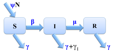
Figure 1 shows the compartment diagram of the SIR model (3.1) with vital dynamics, that is, with demographic (birth and death) effects, and an induced death rate.

Figure 1. Compartment diagram of the SIR model (3.1) with vital dynamics $\psi$ and $\gamma$ and an induced death rate $\gamma_{I}$.

3.2. Analysis of the equilibria

Firstly, we start by analysing the equations (3.1) of the model that serve as the basis for the propagation dynamics of the Ebola virus with death and birth rates. As we shall see (cf. Theorem 3.1), the dynamics are determined by the basic reproduction number

(3.2) $$R_{0}:=\dfrac{\beta N}{\mu+\gamma+\gamma_{I}}.$$

An equilibrium point $E=(S,I,R)\in\mathrm{R}^{3}_{+}$ of (3.1) satisfies, by definition,

(3.3) $$\psi N-\beta SI-\gamma S=0,$$

(3.4) $$\beta SI-\mu I-\left(\gamma+\gamma_{I}\right)I=0,$$

(3.5) $$\mu I-\gamma R=0.$$

There are two biologically meaningful equilibrium points: if $I=0$, then there is no disease for the population, and the equilibrium point is called a disease-free equilibrium; otherwise, if $I>0$, then the equilibrium point is called endemic. By adding equations (3.3) and (3.4), we obtain that

$$\psi N-\gamma S-(\mu+\gamma+\gamma_{I})I=0.$$

Then,

(3.6) $$S=\dfrac{\psi N-(\mu+\gamma+\gamma_{I})I}{\gamma}.$$

From (3.4) and (3.6), we get

$$I\left(\dfrac{\beta\psi N-\gamma\left(\mu+\gamma+\gamma_{I}\right)}{\gamma}-\dfrac{\beta\left(\mu+\gamma+\gamma_{I}\right)}{\gamma}I\right)=0.$$

Therefore, or $I=0$ or

(3.7) $$I=\dfrac{\beta\psi N-\gamma\left(\mu+\gamma+\gamma_{I}\right)}{\beta\left(\mu+\gamma+\gamma_{I}\right)}.$$

If $I=0$, then from (3.6) we obtain that $S=\dfrac{\psi N}{\gamma}$. It follows from (3.5) that $R=0$. We just proved that there is a virus free equilibrium $E_{1}$ given by

(3.8) $$\lim_{t\to\infty}\left(S(t),I(t),R(t)\right)=\left(\dfrac{\psi N}{\gamma},0,0\right)=:E_{1}.$$

If (3.7) holds, then there is another equilibrium with

(3.9) $$I^{*}=\dfrac{\beta\psi N-\gamma\left(\mu+\gamma+\gamma_{I}\right)}{\beta\left(\mu+\gamma+\gamma_{I}\right)}.$$

By substituting (3.9) into (3.6), we obtain that

(3.10) $$S^{*}=\dfrac{\mu+\gamma+\gamma_{I}}{\beta}=\dfrac{N}{R_{0}}$$

and, using (3.5) in (3.6), we get

(3.11) $$R^{*}=\dfrac{\mu}{\gamma}I^{*}=\dfrac{\mu}{\gamma}\left[\dfrac{\beta\psi N-\gamma\left(\mu+\gamma+\gamma_{I}\right)}{\beta\left(\mu+\gamma+\gamma_{I}\right)}\right].$$

We just obtained the endemic equilibrium $E_{2}$ given by

(3.12) $$\lim_{t\to\infty}\left(S(t),I(t),R(t)\right)=\left(S^{*},I^{*},R^{*}\right)=:E_{2},$$

where the expressions of $S^{*}$, $I^{*}$ and $R^{*}$ are given by (3.9)–(3.11). Next result summarizes what we have obtained so far.

Theorem 3.1.

Let $R_{0}$ be the basic reproduction number defined by (3.2). If $R_{0}\leq 1$, then the disease free equilibrium $E_{1}=\left(\dfrac{\psi N}{\gamma},0,0\right)$ of the virus is obtained, which corresponds to the case when the virus dies out (no epidemic). If $R_{0}>1$, then the equilibrium $E_{2}=\left(S^{*},I^{*},R^{*}\right)$ of the virus is obtained, in agreement with expressions (3.9)–(3.11), and the virus is able to invade the population (endemic equilibrium).

3.3. Simulation of the SIR model with demographic effects and an induced death rate

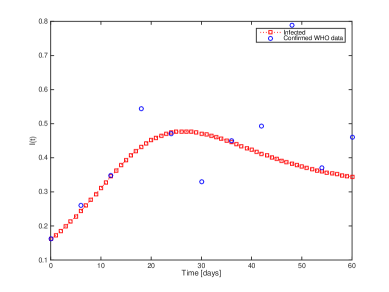
We now present a simulation of the model, taking into account the real outbreak of Ebola virus occurred in Guinea in 2015 and by using the World Health Organization (WHO) data. Precisely, the epidemic data used in our study is borrowed from the WHO web site [35]. The birth rate $\psi=0.03574$ and death rate $\gamma=0.00946$ of the model are obtained from the specific statistical study of the demographic of Guinea in 2015 [31]. The parameters $\beta$, $\mu$, $\gamma$ and $\gamma_{I}$ are obtained by identification by using the real data of WHO. To estimate the parameters of the model, we adapted the initialisation of $I$ with the reported data of WHO by fitting the real data of confirmed cases of infectious in Guinea. The result of fitting is shown in Figure 2. The comparison between the curve of infectious obtained by our simulation and the reported data of confirmed cases by WHO shows that the mathematical model (3.1) fits well the real data by using $\beta=0.19$ as the transmission rate, $\gamma=0.034$ as the infectious rate, $\mu=0.0447$ as the recovered rate, and $\gamma_{I}=0.0353$ as the induced death rate. By comparing the value of $\gamma_{I}$ with the death rate $\gamma$, we remark that $\gamma_{I}=3.735\gamma$. The initial susceptible, infected and recovered populations, are given by

(3.13) $$S(0)=0.8387,\quad I(0)=0.1613,\quad R(0)=0,$$

respectively. The choice of $I(0)$ is in agreement with the data shown in Figure 2 of the WHO data. By using the value of Guinea’s population, which is estimated at $P=11780162$ in $2015$, and the number of confirmed infectious cases (obtained from WHO), the initialization of $I(0)$ corresponds to the number of infected divided by the total number of population. Then, in reality, the initial number of infected, in the period between January 2015 and March 2015, is given by $0.1613\times P=1900000$, that is, the number of confirmed infectious cases represents $16.13\%$ of the total of population. Figure 2 presents the curve of infectious individuals $I(t)$ simulated by using (3.1) and obtained from the WHO real data.

Figure 2. Graph of infected obtained from (3.1)–(3.13) versus the real data of confirmed cases for the 2015 Ebola outbreak occurred in Guinea between January and March 2015.

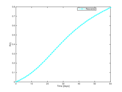
The evolution of susceptible, infected and recovered groups over time, is shown in Figure 3.

(a) $S(t)$ with $S(0)=0.8387$

(b) $I(t)$ with $I(0)=0.1613$

(c) $R(t)$ with $R(0)=0$

Figure 3. Evolution of individuals in compartments $S(t)$, $I(t)$ and $R(t)$ of the SIR model (3.1) with vital dynamics and an induced death rate.

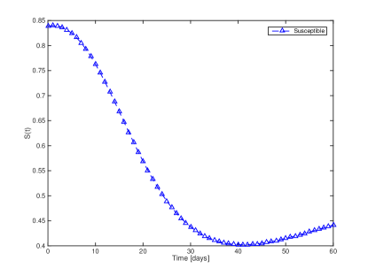
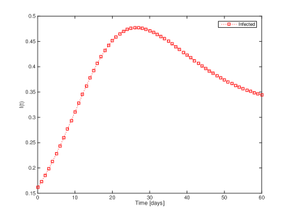
We also studied numerically the equilibria, by solving numerically the SIR model (3.1) with the same parameters and the same initialization. Figure 4a shows the evolution of the susceptible individuals $S(t)$ over time. We see that the oscillations in the numbers of the three compartments damp out over time, eventually reaching an equilibrium. In our mathematical analysis of the model, we found that the equilibrium $S^{*}$ is computed theoretically by (3.10). When we calculate the value of this theoretical result, we find $S^{*}=0.47$, which is equal to the $S^{*}$ computed by the numerical resolution of the model. Figure 4b shows the evolution of the infected individuals $I(t)$ over time. We know that the equilibrium $I^{*}$ is given by (3.9). When we calculate the value of this theoretical result, we find $I^{*}=0.34$, which agrees with the value computed by the numerical resolution of the model. Figure 4c shows the evolution of the recovered individuals $R(t)$ over time. The equilibrium $R^{*}$ is in this case computed theoretically by (3.11), which coincides the value $R^{*}=1.65$ computed numerically.

(a) $S(t)$

(b) $I(t)$

(c) $R(t)$

Figure 4. Evolution of individuals in compartments $S(t)$, $I(t)$ and $R(t)$ of the SIR model (3.1) with vital dynamics and an induced death rate, where the endemic equilibrium is given by $\left(S^{*}(t),I^{*}(t),R^{*}(t)\right)=\left(0.47,0.34,1.65\right)$.

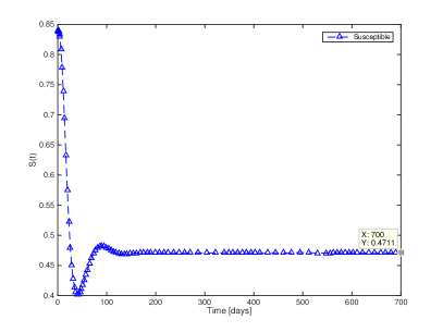
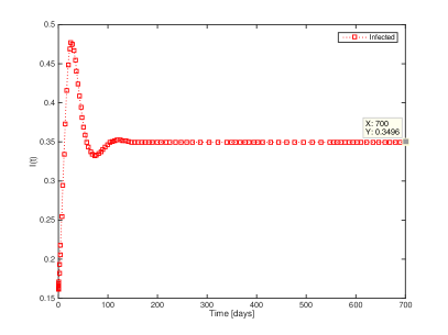
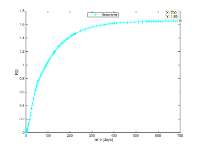
The fact that the reached equilibrium $(S^{*},I^{*},R^{*})$ computed theoretically coincides with the value found by the numerical simulation of the model, is a validation of our study of the SIR model with vital dynamics and induced death rate, which describes well the currently detection of Ebola virus in Guinea.

4. Optimal control of the virus under vital dynamics

Nowadays there are several trial vaccinations against Ebola. One was already applied in Guinea and seems highly effective [36]. In this section, we present a strategy for the control of the virus, by introducing into the model (3.1) a control $u(t)$ representing the vaccination rate at time $t$. The control $u(t)$ is the fraction of susceptible individuals being vaccinated per unit of time, taking values on the interval $[0,0.9]$. Then, the mathematical model with control is given by the following system of non-linear differential equations:

(4.1) $$\begin{cases}\dfrac{dS(t)}{dt}=\psi N-\beta S(t)I(t)-\gamma S(t)-u(t)S(t),\\[5.69046pt] \dfrac{dI(t)}{dt}=\beta S(t)I(t)-\mu I(t)-(\gamma+\gamma_{I})I(t),\\[5.69046pt] \dfrac{dR(t)}{dt}=\mu I(t)-\gamma R(t)+u(t)S(t).\end{cases}$$

The goal of the strategy is to reduce the infected individuals and the cost of vaccination. Precisely, the optimal control problem consists of minimizing the objective functional

(4.2) $$J(u)=\int_{0}^{t_{end}}\left[I(t)+\dfrac{\tau}{2}u^{2}(t)\right]dt,$$

where $u$ is the control variable, $u(t)\in[0,0.9]$, which represents the vaccination rate at time $t$, and the parameters $\tau$ and $t_{end}$ denote, respectively, the weight on cost and the duration of the vaccination program. In the quadratic term of (4.2), $\tau$ is a positive weight parameter associated with the control $u(t)$ and the square of the control variable reflects the severity of the side effects of the vaccination. One has $u\in\mathcal{U}_{ad}$, where

$$\mathcal{U}_{ad}=\left\{u:u\,\text{is measurable},0\leq u(t)\leq u_{max}<\infty,\,t\in[0,t_{end}]\right\}$$

is the admissible control set with $u_{max}=0.9$. The existence of an optimal solution follows from Theorem 2.1 of [16] (see also the study of the spread of influenza A (H1N1) [13] by using the SIR model).

In our study of the control of the virus, we use the parameters defined in Section 3.3. For the numerical simulations of the optimal control problem, we have used the ACADO solver [4], which is based on a multiple shooting method, including automatic differentiation and based ultimately on the semidirect multiple shooting algorithm of Bock and Pitt [6]. The ACADO solver comes as a self-contained public domain software environment, written in C++, for automatic control and dynamic optimization. Because (4.1) is a nonlinear control system, functional (4.2) is quadratic in the control and linear in the phase variable $I$, it is not clear that the numerically found solution through ACADO to our optimal control problem gives the global minimum to the functional (4.2), or only a local one. Indeed, with ACADO the optimal control problem is approximated by a finite dimensional optimization problem, which is then solved by techniques from mathematical programming. This only gives a candidate for local minimizer. Because of this, we have also used a dynamic programming approach and checked our results by solving it with BocopHJB, which is a C/C++ toolbox for optimal control developed since 2014 in the framework of the Inria–Saclay initiative for an open source optimal control toolbox, being supported by the team “Commands” (see http://bocop.org). While ACADO implements a local optimization method, the package BocopHJB implements a global optimization method. Similarly to the dynamic programming approach, the optimal control problem is solved by BocopHJB in two steps: first the Hamilton–Jacobi–Bellman equation satisfied by the value function of the problem is solved; then the optimal trajectory is simulated from any chosen initial condition [7]. The obtained results through BocopHJB are coincident with those obtained through ACADO and, because of that, we claim to have found the global minimum to the problem.

(a) Susceptible $S(t)$

(b) Recovered $R(t)$

(c) Infected $I(t)$

Figure 5. Comparison between the curves of individuals in case of optimal control (4.1)–(4.2) with $\tau=0.02$ versus without control.

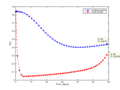
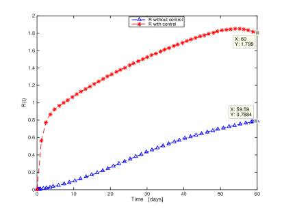
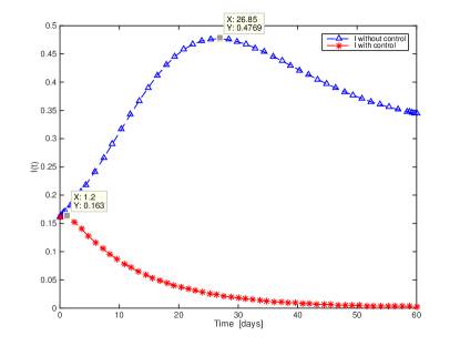
Figure 5 shows the significant difference in the number of susceptible, recovered, and infected individuals with and without control. In Figure 5a, we see that the number of susceptible $S$, in case of optimal control, decreases faster during the vaccination campaign. It reaches 34.78% at the end of the campaign against 44.12% in the absence of optimal control. Figure 5b shows that the number of recovered individuals increases rapidly. The number $R(t_{end})$ increases more rapidly in case of control than without control. In Figure 5c, the time-dependent curve of infected individuals shows that the peak of the curve of infected individuals is less important in case of control. In fact, the maximum value on the infected curve $I$ under optimal control is 16.3%, against 47.69% without any control (see Figure 5c). The other important effect of control, which we can see in the same curve, is the period of infection, which is less important in case of control of the virus. The value of the period of infection is $46$ days in case of optimal control, versus more than $60$ days without vaccination. This shows the efficiency of vaccination in controlling Ebola.

Figure 6. Optimal control function $u(t)$ for problem (4.1)–(4.2) with initial conditions (3.13), $t\in[0,t_{end}]$, $t_{end}=60$ days, and $\tau=0.02$.

Figure 7. Total population $N(t)=S(t)+I(t)+R(t)$, in case of optimal control (4.1)–(4.2) versus without control (3.1).

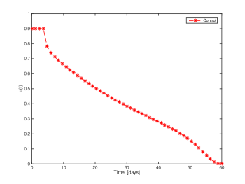
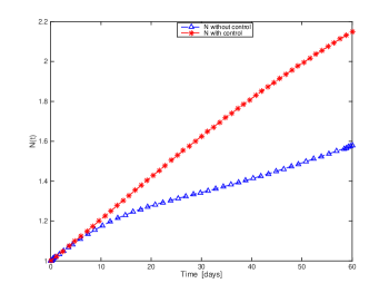
In conclusion, one can say that Figure 5 shows the effectiveness of optimal vaccination in controlling Ebola. Figure 6 gives a representation of the optimal control $u(t)$; while Figure 7 shows the evolution of the number of total population $N(t)=S(t)+I(t)+R(t)$ over time. We see that the total number of population is bigger in case of vaccination (less people dying).

5. Conclusion

Mathematical modelling of the detection of a virulent virus such Ebola is a powerful tool to understand the dynamics of the propagation of the virus in a population. The main aim is to provide useful predictions about the potential transmission of the virus. The important step after modelling is to study the properties of the system of equations that describes the propagation of the virus. In this work, we analysed a SIR model with vital dynamics for the early detection of Ebola virus in West Africa, by adding demographic effects and an induced death rate, in order to discuss when the model makes sense mathematically and to study the information provided by the model. We simulated the model in the case of a basic reproduction number $R_{0}>1$, which describes the current situation of Ebola virus in Guinea. We studied the equilibria. The system of equations of the model was solved numerically and the numerical simulations confirmed the theoretical analysis of the equilibria for the model. Finally, we controlled the propagation of the virus by minimizing the number of infected individuals and the cost of vaccination and showing the importance of optimal control.

References

- [1] J. Alton, The Ebola survival handbook, Skyhorse Publishing, New York, 2014.
- [2] I. Area, H. Batarfi, J. Losada, J. J. Nieto, W. Shammakh and A. Torres, On a fractional order Ebola epidemic model, Adv. Difference Equ. 2015 (2015), no. 278, 12 pp.
- [3] I. Area, J. Losada, F. Ndaïrou, J. J. Nieto and D. D. Tcheutia, Mathematical modeling of 2014 Ebola outbreak, Math. Methods Appl. Sci., in press. DOI: 10.1002/mma.3794.
- [4] D. Ariens, M. Diehl, H. J. Ferreau, B. Houska, F. Logist, R. Quirynen and M. Vukov, ACADO Toolkit User’s Manual, Optimization in Engineering Center (OPTEC) and Department of Electrical Engineering, KU Leuven, 2014.
- [5] M. Barry, F. A. Traoré, F. B. Sako, D. O. Kpamy, E. I. Bah, M. Poncin, S. Keita, M. Cisse and A. Touré, Ebola outbreak in Conakry, Guinea: Epidemiological, clinical, and outcome features, Médecine et Maladies Infectieuses 44 (2014), no. 11–12, 491–494.
- [6] H. G. Bock and K. J. Pitt, A multiple shooting algorithm for direct solution of optimal control problems, Proc. 9th IFAC World Congress, Budapest, Pergamon Press, 1984, 243–247.
- [7] F. Bonnans, D. Giorgi, B. Heymann, P. Martinon and O. Tissot, BocopHJB 1.0.1 – User Guide, Inria Saclay, CMAP Ecole Polytechnique and LPMA, Sorbonne University, Paris, 2015.
- [8] L. Borio et al. [Working Group on Civilian Biodefense; Corporate Author], Hemorrhagic fever viruses as biological weapons: medical and public health management, Journal of the American Medical Association 287 (2002), no. 18, 2391–2405.
- [9] F. Brauer, P. V. Driessche and J. Wu, Mathematical Epidemiology, Lectures Notes in Mathematics 1945, Mathematical Biosciences Subseries, 2008.
- [10] E. Chapnick, Ebola Myths & Facts, John Wiley & Sons, Inc., Hoboken, New Jersey, 2015.
- [11] O. Diekmann, H. Heesterbeek and T. Britton, Mathematical tools for understanding infectious disease dynamics, Princeton Series in theoretical and Computational Biology, 2013.
- [12] S. F. Dowell, R. Mukunu, T. G. Ksiazek, A. S. Khan, P. E. Rollin and C. J. Peters, Transmission of Ebola hemorrhagic fever: a study of risk factors in family members, Kikwit, Democratic Republic of the Congo, 1995. Commission de Lutte contre les Epidémies à Kikwit. J. Infect. Dis. 179 (1999), Suppl. 1, S87–S91.
- [13] M. El hia, O. Balatif, J. Bouyaghroumni, E. Labriji and M. Rachik, Optimal control applied to the spread of influenza A(H1N1), Appl. Math. Sci. (Ruse) 6 (2012), no. 81-84, 4057–4065.
- [14] H. Gaff and E. Schaefer, Optimal control applied to vaccination and treatment strategies for various epidemiological models, Math. Biosci. Eng. 6 (2009), no. 3, 469–492.
- [15] H. W. Hethcote, The mathematics of infectious diseases, SIAM Rev. 42 (2000), no. 4, 599–653.
- [16] H. R. Joshi, S. Lenhart, M. Y. Li and L.Wang, Optimal control methods applied to disease models, in Mathematical studies on human disease dynamics, 187–207, Contemp. Math., 410, Amer. Math. Soc., Providence, RI, 2006.
- [17] M. Kretzschmar, Ring vaccination and smallpox control, Emerging Infectious Diseases 10 (2004), no. 5, 832–841.
- [18] J. Legrand, R. F. Grais, P. Y. Boelle, A. J. Valleron and A. Flahault, Understanding the dynamics of Ebola epidemics, Epidemiol. Infect. 135 (2007), no. 4, 610–621.
- [19] J. A. Lewnard, M. L. Ndeffo Mbah, J. A. Alfaro-Murillo, F. L. Altice, L. Bawo, T. G. Nyenswah and A. P. Galvani, Dynamics and control of Ebola virus transmission in Montserrado, Liberia: A mathematical modelling analysis, The Lancet Infectious Diseases 14 (2014), no. 12, 1189–1195.
- [20] I. M. Longini Jr. and E. Ackerman, An optimization model for influenza A epidemics, Mathematical Biosciences 38 (1978), no. 1-2, 141–157.
- [21] C. J. Peters and J. W. LeDuc, An introduction to Ebola: The virus and the disease, Journal of Infectious Diseases 179 (1999), Suppl. 1, ix–xvi.
- [22] A. Rachah and D. F. M. Torres, Mathematical modelling, simulation and optimal control of the 2014 Ebola outbreak in West Africa, Discrete Dyn. Nat. Soc. 2015 (2015), Art. ID 842792, 9 pp. arXiv:1503.07396
- [23] A. Rachah and D. F. M. Torres, Optimal control strategies for the spread of Ebola in West Africa, J. Math. Anal. 7 (2016), no. 1, 102–114. arXiv:1512.03395
- [24] A. Rachah and D. F. M. Torres, Dynamics and optimal control of Ebola transmission, Math. Comput. Sci., in press. arXiv:1603.03265
- [25] A. Rachah and D. F. M. Torres, Predicting and controlling the Ebola infection, Math. Methods Appl. Sci., in press. DOI:10.1002/mma.3841 arXiv:1511.06323
- [26] Report of an International Commission, Ebola haemorrhagic fever in Zaire, 1976, Bull. World Health Organ. 56 (1978), no. 2, 271–293.
- [27] H. S. Rodrigues, M. T. T. Monteiro and D. F. M. Torres, Dynamics of dengue epidemics when using optimal control, Math. Comput. Modelling 52 (2010), no. 9-10, 1667–1673. arXiv:1006.4392
- [28] H. S. Rodrigues, M. T. T. Monteiro and D. F. M. Torres, Vaccination models and optimal control strategies to dengue, Math. Biosci. 247 (2014), 1–12. arXiv:1310.4387
- [29] T. C. Smith, Ebola. Deadly Diseases and Epidemics, Chelsea House Publisher, 2006.
- [30] T. C. Smith, Ebola and Marburg Virus, Second Edition, Deadly diseases and epidemics, Chelsea House Publisher, 2010.
- [31] Statistiques mondiales, Guinée Conakry, http://www.statistiques-mondiales.com/guinee.htm.
- [32] Uganda Ministry of Health, An outbreak of Ebola in Uganda, Trop. Med. Int. Health. 7 (2002), no. 12, 1068–1075.
- [33] X.-S. Wang and L. Zhong, Ebola outbreak in West Africa: real-time estimation and multiple-wave prediction, Math. Biosci. Eng. 12 (2015), no. 5, 1055–1063.
- [34] WHO, World Health Organization, Report of an International Study Team, Ebola haemorrhagic fever in Sudan 1976, Bull. World Health Organ. 56 (1978), no. 2, 247–270.
- [35] WHO, World Health Organization, Ebola data and statistics, http://apps.who.int/gho/data/node.ebola-sitrep.other-affected.
- [36] WHO, World Health Organization, Guinea: Ebola vaccine trial, http://www.who.int/features/2015/guinea-ebola-vaccine/en