General scan in flavor parameter space in the models with vector quark doublets and an enhancement in BXsγ𝐵subscript𝑋𝑠𝛾B\to X_{s}\gamma process

Wenyu Wang, Zhao-Hua Xiong, Xin-Yan Zhao Institute of Theoretical Physics, Beijing University of Technology, Beijing 100124, China
Abstract

In the models with vector like quark doublets, the mass matrices of up and down type quarks are related. Precise diagonalization for the mass matrices becames an obstacle in the numerical studies. In this work we propose a diagonalization method at first. As its application, in the standard model with one vector like quark doublet we present quark mass spectrum, Feynman rules for the calculation of BXsγ𝐵subscript𝑋𝑠𝛾B\to X_{s}\gamma. We find that i) under the constraints of the CKM matrix measurements, the mass parameters in the bilinear term are constrained to a small value by the small deviation from unitarity; ii) compared with the fourth generation extension of the standard model, there is an enhancement to BXsγ𝐵subscript𝑋𝑠𝛾B\to X_{s}\gamma process in the contribution of vector like quark, resulting a non-decoupling effect in such models.

pacs:
12.15.-g, 12,15.Ff, 13.20.He

I Introduction

Though the standard model (SM) has been verified to be correct times by times, many new physics beyond standard model are proposed to solve both experimental and aesthetical problems, such as neutrino masses, μ𝜇\mu anomalous magnetic movement problem or hierarchy problem, etc. Many new models introduce vector like particles (VLP) VLP-rev whose right handed and left handed components transform in the same way under the weak SU(2)×\timesU(1) gauge group. The extension is acceptable because the anomalies generated by the VLPs cancel automatically, and vector quarks can be heavy naturally. VLPs also arise in some grand unification theories. For example, in order to explain the little hierarchy problem between the traditional GUT scale and string scale, a testable flipped SU(5)×U(1)X𝑆𝑈5𝑈subscript1𝑋SU(5)\times U(1)_{X} model are proposed in Ref. Jiang:2009zza in which the TeV-scale VLPs were introduced Jiang:2006hf . Such kind of models can be constructed from the free fermionic string constructions at the Kac-Moody level one Antoniadis:1988tt ; Lopez:1992kg and from the local F-theory model Beasley:2008dc ; Jiang:2009zza .

However when we do the flavor physics with doublet VLPs in these models Li:2012xz ; Li:2015nya , a problem always appears when we are dealing with the mass spectrum of quarks and leptons. Let us start with the SM in which all fermion masses come from the Yukawa couplings. After the spontaneously gauge symmetry breaking, we can get two separate mass matrices MU,MDsubscript𝑀𝑈subscript𝑀𝐷M_{U},~{}M_{D} for the up and down type fermions. The mass eigen states are obtained after the diagonalization

ZUMUUU=MUD,ZDMDUD=MDD,formulae-sequencesuperscriptsubscript𝑍𝑈subscript𝑀𝑈subscript𝑈𝑈superscriptsubscript𝑀𝑈𝐷superscriptsubscript𝑍𝐷subscript𝑀𝐷subscript𝑈𝐷superscriptsubscript𝑀𝐷𝐷\displaystyle Z_{U}^{\dagger}M_{U}U_{U}=M_{U}^{D},~{}~{}Z_{D}^{\dagger}M_{D}U_{D}=M_{D}^{D}, (1)

where MUD=diag.[mu,mc,mt]formulae-sequencesuperscriptsubscript𝑀𝑈𝐷diagsubscript𝑚𝑢subscript𝑚𝑐subscript𝑚𝑡M_{U}^{D}={\rm diag.}[m_{u},m_{c},m_{t}], MDD=diag.[md,ms,mb]formulae-sequencesuperscriptsubscript𝑀𝐷𝐷diagsubscript𝑚𝑑subscript𝑚𝑠subscript𝑚𝑏M_{D}^{D}={\rm diag.}[m_{d},m_{s},m_{b}]. The physical measurable parameters are misubscript𝑚𝑖m_{i} and the so called CKM matrix

VCKM=UUUD.subscript𝑉CKMsuperscriptsubscript𝑈𝑈subscript𝑈𝐷V_{\rm CKM}=U_{U}^{\dagger}U_{D}. (2)

Since MU,MDsubscript𝑀𝑈subscript𝑀𝐷M_{U},~{}M_{D} come from separate Yukawa couplings, we can always set one of the matrices diagonal, for example MUsubscript𝑀𝑈M_{U}, and use the CKM matrix to get the Yukawa couplings

ZD(md000ms000mb)VCKM=(Y11DvY12DvY13DvY21DvY22DvY23DvY31DvY32DvY33Dv)subscript𝑍𝐷subscript𝑚𝑑000subscript𝑚𝑠000subscript𝑚𝑏superscriptsubscript𝑉CKMsubscriptsuperscript𝑌𝐷11𝑣subscriptsuperscript𝑌𝐷12𝑣subscriptsuperscript𝑌𝐷13𝑣subscriptsuperscript𝑌𝐷21𝑣subscriptsuperscript𝑌𝐷22𝑣subscriptsuperscript𝑌𝐷23𝑣subscriptsuperscript𝑌𝐷31𝑣subscriptsuperscript𝑌𝐷32𝑣subscriptsuperscript𝑌𝐷33𝑣\displaystyle Z_{D}\left(\begin{array}[]{ccc}m_{d}&0&0\\ 0&m_{s}&0\\ 0&0&m_{b}\end{array}\right)V_{\rm CKM}^{\dagger}=\left(\begin{array}[]{ccc}Y^{D}_{11}v&Y^{D}_{12}v&Y^{D}_{13}v\\ Y^{D}_{21}v&Y^{D}_{22}v&Y^{D}_{23}v\\ Y^{D}_{31}v&Y^{D}_{32}v&Y^{D}_{33}v\end{array}\right) (9)

for the calculation in flavor physics. Note that v𝑣v is the vacuum expectation value (VEV) of the Higgs, and ZDsubscript𝑍𝐷Z_{D} is a random unitary matrix.

Such a trick can not be used in case of the participation of a vector doublet, namely Q𝑄Q with gauge charge 𝟑,𝟐,𝟏𝟔3216\bf 3,~{}2,~{}\frac{1}{6} and Q¯¯𝑄\bar{Q} with gauge charge 𝟑¯,𝟐,𝟏𝟔¯3216\bf\bar{3},~{}2,~{}-\frac{1}{6}, resulting bilinear term in the lagrangian

MVQQ¯.superscript𝑀𝑉𝑄¯𝑄M^{V}Q\cdot\bar{Q}.

It is clear that in the model, there are the same input parameters in the matrices MU,MDsubscript𝑀𝑈subscript𝑀𝐷M_{U},~{}M_{D}

MUsubscript𝑀𝑈\displaystyle M_{U} =\displaystyle= (Y11UvY12UvY13UvY21UvY22UvY23UvY31UvY32UvY33UvM41VM42VM43V),MD=(Y11DvY12DvY13DvY21DvY22DvY23DvY31DvY32DvY33DvM41VM42VM43V).subscriptsuperscript𝑌𝑈11𝑣subscriptsuperscript𝑌𝑈12𝑣subscriptsuperscript𝑌𝑈13𝑣subscriptsuperscript𝑌𝑈21𝑣subscriptsuperscript𝑌𝑈22𝑣subscriptsuperscript𝑌𝑈23𝑣subscriptsuperscript𝑌𝑈31𝑣subscriptsuperscript𝑌𝑈32𝑣subscriptsuperscript𝑌𝑈33𝑣subscriptsuperscript𝑀𝑉41subscriptsuperscript𝑀𝑉42subscriptsuperscript𝑀𝑉43subscript𝑀𝐷subscriptsuperscript𝑌𝐷11𝑣subscriptsuperscript𝑌𝐷12𝑣subscriptsuperscript𝑌𝐷13𝑣subscriptsuperscript𝑌𝐷21𝑣subscriptsuperscript𝑌𝐷22𝑣subscriptsuperscript𝑌𝐷23𝑣subscriptsuperscript𝑌𝐷31𝑣subscriptsuperscript𝑌𝐷32𝑣subscriptsuperscript𝑌𝐷33𝑣subscriptsuperscript𝑀𝑉41subscriptsuperscript𝑀𝑉42subscriptsuperscript𝑀𝑉43\displaystyle\left(\begin{array}[]{cccc}Y^{U}_{11}v&Y^{U}_{12}v&Y^{U}_{13}v&\cdots\\ Y^{U}_{21}v&Y^{U}_{22}v&Y^{U}_{23}v&\cdots\\ Y^{U}_{31}v&Y^{U}_{32}v&Y^{U}_{33}v&\cdots\\ M^{V}_{41}&M^{V}_{42}&M^{V}_{43}&\cdots\end{array}\right),~{}M_{D}=\left(\begin{array}[]{cccc}Y^{D}_{11}v&Y^{D}_{12}v&Y^{D}_{13}v&\cdots\\ Y^{D}_{21}v&Y^{D}_{22}v&Y^{D}_{23}v&\cdots\\ Y^{D}_{31}v&Y^{D}_{32}v&Y^{D}_{33}v&\cdots\\ -M^{V}_{41}&-M^{V}_{42}&-M^{V}_{43}&\cdots\end{array}\right). (18)

The mass matrices for up and down type quarks are related to each other. Therefore, we can not set one of the matrices diagonal and the CKM matrix can not be got easily. The shooting method is always used to treat such an obstacle. Random MUsubscript𝑀𝑈M_{U} and MDsubscript𝑀𝐷M_{D} are generated to meet the requirements after diagonlization: the mass of eigen state and the measurements of elements of CKM matrix. However this is too much time consuming, and precise solution for diagonalization is almost unavailable. Although this is just a numerical problem, when one treats the VLP contributions to the flavor physics seriously, diagonalization of quark matrices will be the first and important step.

In this paper, we will first propose a general method to solve the obstacle in models with vector like quark doublets. As its application, we will study rare B decay BXsγ𝐵subscript𝑋𝑠𝛾B\to X_{s}\gamma in the SM with one vector like quark doublet. The paper is organized as follows. We show the detail of the trick in Section 2. The simple application to BXsγ𝐵subscript𝑋𝑠𝛾B\to X_{s}\gamma process, including quark mass spectrum, Feynman rules and the Wilson coefficients, as well as the numerical analysis for calculation of BXsγ𝐵subscript𝑋𝑠𝛾B\to X_{s}\gamma is shown in Section 3. A summary is given in Section 4.

II The Trick of diagonalization of vector quark doublet

Firstly, we address the problem clearly on how to deal with the diagonalization of N×N𝑁𝑁N\times N matrix MUsubscript𝑀𝑈M_{U} and MDsubscript𝑀𝐷M_{D}:

ZUMUUU=MUD,ZDMDUD=MDDformulae-sequencesuperscriptsubscript𝑍𝑈subscript𝑀𝑈subscript𝑈𝑈superscriptsubscript𝑀𝑈𝐷superscriptsubscript𝑍𝐷subscript𝑀𝐷subscript𝑈𝐷superscriptsubscript𝑀𝐷𝐷\displaystyle Z_{U}^{\dagger}M_{U}U_{U}=M_{U}^{D},~{}Z_{D}^{\dagger}M_{D}U_{D}=M_{D}^{D} (19)

in which MUD,MDDsuperscriptsubscript𝑀𝑈𝐷superscriptsubscript𝑀𝐷𝐷M_{U}^{D},M_{D}^{D} are the diagonal mass matrices for up and down type quark, respectively. Note that N𝑁N should be greater than 3 and the first three elements in the matices should be the three generations of quark multiplates in the SM, other elments with N>3𝑁3N>3 are the new multiplates introduced in new physics beyond the SM. Then we have

MU=(Y11UvY12UvY13UvMU1NY21UvY22UvY23UvMU2NY31UvY32UvY33UvMU3NMN1VMN2VMN3VMUNN),MD=(Y11DvY12DvY13DvMD1NY21DvY22DvY23DvMD2NY31DvY32DvY33DvMD3NMN1VMN2VMN3VMDNN).formulae-sequencesubscript𝑀𝑈subscriptsuperscript𝑌𝑈11𝑣subscriptsuperscript𝑌𝑈12𝑣subscriptsuperscript𝑌𝑈13𝑣subscript𝑀𝑈1𝑁subscriptsuperscript𝑌𝑈21𝑣subscriptsuperscript𝑌𝑈22𝑣subscriptsuperscript𝑌𝑈23𝑣subscript𝑀𝑈2𝑁subscriptsuperscript𝑌𝑈31𝑣subscriptsuperscript𝑌𝑈32𝑣subscriptsuperscript𝑌𝑈33𝑣subscript𝑀𝑈3𝑁subscriptsuperscript𝑀𝑉𝑁1subscriptsuperscript𝑀𝑉𝑁2subscriptsuperscript𝑀𝑉𝑁3subscript𝑀𝑈𝑁𝑁subscript𝑀𝐷subscriptsuperscript𝑌𝐷11𝑣subscriptsuperscript𝑌𝐷12𝑣subscriptsuperscript𝑌𝐷13𝑣subscript𝑀𝐷1𝑁subscriptsuperscript𝑌𝐷21𝑣subscriptsuperscript𝑌𝐷22𝑣subscriptsuperscript𝑌𝐷23𝑣subscript𝑀𝐷2𝑁subscriptsuperscript𝑌𝐷31𝑣subscriptsuperscript𝑌𝐷32𝑣subscriptsuperscript𝑌𝐷33𝑣subscript𝑀𝐷3𝑁subscriptsuperscript𝑀𝑉𝑁1subscriptsuperscript𝑀𝑉𝑁2subscriptsuperscript𝑀𝑉𝑁3subscript𝑀𝐷𝑁𝑁\displaystyle M_{U}=\left(\begin{array}[]{ccccc}Y^{U}_{11}v&Y^{U}_{12}v&Y^{U}_{13}v&\cdots&M_{U1N}\\ Y^{U}_{21}v&Y^{U}_{22}v&Y^{U}_{23}v&\cdots&M_{U2N}\\ Y^{U}_{31}v&Y^{U}_{32}v&Y^{U}_{33}v&\cdots&M_{U3N}\\ \cdots&\cdots&\cdots&\cdots&\cdots\\ M^{V}_{N1}&M^{V}_{N2}&M^{V}_{N3}&\cdots&M_{UNN}\end{array}\right),~{}M_{D}=\left(\begin{array}[]{ccccc}Y^{D}_{11}v&Y^{D}_{12}v&Y^{D}_{13}v&\cdots&M_{D1N}\\ Y^{D}_{21}v&Y^{D}_{22}v&Y^{D}_{23}v&\cdots&M_{D2N}\\ Y^{D}_{31}v&Y^{D}_{32}v&Y^{D}_{33}v&\cdots&M_{D3N}\\ \cdots&\cdots&\cdots&\cdots&\cdots\\ -M^{V}_{N1}&-M^{V}_{N2}&-M^{V}_{N3}&\cdots&M_{DNN}\end{array}\right). (30)

The last line of the two matrices has the same parameters except the last elements.

Considering that there are some same parameters in MUsubscript𝑀𝑈M_{U} and MDsubscript𝑀𝐷M_{D}, we find that a very simple way is to add two matrices in Eq. (30)

MU+MD=(ZUMUDUCKMN+ZDMDD)UD.subscript𝑀𝑈subscript𝑀𝐷subscript𝑍𝑈subscriptsuperscript𝑀𝐷𝑈subscript𝑈CKMNsubscript𝑍𝐷subscriptsuperscript𝑀𝐷𝐷subscriptsuperscript𝑈𝐷\displaystyle M_{U}+M_{D}=\left(Z_{U}M^{D}_{U}U_{\rm CKMN}+Z_{D}M^{D}_{D}\right)U^{\dagger}_{D}. (31)

The left side of the equation is

MU+MD=(Y11Uv+Y11DvY12Uv+Y12DvY13Uv+Y13DvMU1N+MD1NY21Uv+Y21DvY22Uv+Y22DvY23Uv+Y23DvMU2N+MD2NY31Uv+Y31DvY32Uv+Y32DvY33Uv+Y33DvMU3N+MD3N000MUNN+MDNN).subscript𝑀𝑈subscript𝑀𝐷subscriptsuperscript𝑌𝑈11𝑣subscriptsuperscript𝑌𝐷11𝑣subscriptsuperscript𝑌𝑈12𝑣subscriptsuperscript𝑌𝐷12𝑣subscriptsuperscript𝑌𝑈13𝑣subscriptsuperscript𝑌𝐷13𝑣subscript𝑀𝑈1𝑁subscript𝑀𝐷1𝑁subscriptsuperscript𝑌𝑈21𝑣subscriptsuperscript𝑌𝐷21𝑣subscriptsuperscript𝑌𝑈22𝑣subscriptsuperscript𝑌𝐷22𝑣subscriptsuperscript𝑌𝑈23𝑣subscriptsuperscript𝑌𝐷23𝑣subscript𝑀𝑈2𝑁subscript𝑀𝐷2𝑁subscriptsuperscript𝑌𝑈31𝑣subscriptsuperscript𝑌𝐷31𝑣subscriptsuperscript𝑌𝑈32𝑣subscriptsuperscript𝑌𝐷32𝑣subscriptsuperscript𝑌𝑈33𝑣subscriptsuperscript𝑌𝐷33𝑣subscript𝑀𝑈3𝑁subscript𝑀𝐷3𝑁000subscript𝑀𝑈𝑁𝑁subscript𝑀𝐷𝑁𝑁\displaystyle M_{U}+M_{D}=\left(\begin{array}[]{ccccc}Y^{U}_{11}v+Y^{D}_{11}v&Y^{U}_{12}v+Y^{D}_{12}v&Y^{U}_{13}v+Y^{D}_{13}v&\cdots&M_{U1N}+M_{D1N}\\ Y^{U}_{21}v+Y^{D}_{21}v&Y^{U}_{22}v+Y^{D}_{22}v&Y^{U}_{23}v+Y^{D}_{23}v&\cdots&M_{U2N}+M_{D2N}\\ Y^{U}_{31}v+Y^{D}_{31}v&Y^{U}_{32}v+Y^{D}_{32}v&Y^{U}_{33}v+Y^{D}_{33}v&\cdots&M_{U3N}+M_{D3N}\\ \cdots&\cdots&\cdots&\cdots&\cdots\\ 0&0&0&\cdots&M_{UNN}+M_{DNN}\end{array}\right). (37)

Obviously, the mass inputs from bilinear terms vanish. We can denote the matrix in the form as

MU+MD=MUD=(𝐌𝐀𝐌𝐁𝐌𝟎MC),subscript𝑀𝑈subscript𝑀𝐷subscript𝑀𝑈𝐷subscript𝐌𝐀subscript𝐌𝐁subscript𝐌0subscript𝑀𝐶\displaystyle M_{U}+M_{D}=M_{UD}=\left(\begin{array}[]{cc}{\bf M_{A}}&{\bf M_{B}}\\ {\bf M_{0}}&M_{C}\end{array}\right), (40)

in which 𝐌𝐀subscript𝐌𝐀{\bf M_{A}}, 𝐌𝐁subscript𝐌𝐁{\bf M_{B}}, 𝐌𝟎subscript𝐌0{\bf M_{0}} are (N1)×(N1)𝑁1𝑁1(N-1)\times(N-1), (N1)×1𝑁11(N-1)\times 1 and 1×(N1)1𝑁11\times(N-1) matrices correspondingly.

To prepare for the diagonalization, we chose the diagonal mass matrix elements of quarks (mu,mc,mt,mX)subscript𝑚𝑢subscript𝑚𝑐subscript𝑚𝑡subscript𝑚𝑋(m_{u},m_{c},m_{t},\cdots m_{X}), (md,ms,mb,,mY)subscript𝑚𝑑subscript𝑚𝑠subscript𝑚𝑏subscript𝑚𝑌(m_{d},m_{s},m_{b},\cdots,m_{Y}) and a matrix UCKMNsubscript𝑈CKMNU_{\rm CKMN}, which are determined partly by experimental measurements as input parameters

UCKMNsubscript𝑈CKMN\displaystyle U_{\rm CKMN} =\displaystyle= UUUD=((UCKM)3×3UNN)=((UudUusUubUcdUcsUcbUtdUtsUtb)UNN).subscriptsuperscript𝑈𝑈subscript𝑈𝐷subscriptsubscript𝑈CKM33subscript𝑈𝑁𝑁subscript𝑈𝑢𝑑subscript𝑈𝑢𝑠subscript𝑈𝑢𝑏subscript𝑈𝑐𝑑subscript𝑈𝑐𝑠subscript𝑈𝑐𝑏subscript𝑈𝑡𝑑subscript𝑈𝑡𝑠subscript𝑈𝑡𝑏subscript𝑈𝑁𝑁\displaystyle U^{\dagger}_{U}U_{D}=\left(\begin{array}[]{cc}\left(U_{\rm CKM}\right)_{3\times 3}&\cdots\\ \cdots&U_{NN}\end{array}\right)=\left(\begin{array}[]{cc}\left(\begin{array}[]{ccc}U_{ud}&U_{us}&U_{ub}\\ U_{cd}&U_{cs}&U_{cb}\\ U_{td}&U_{ts}&U_{tb}\end{array}\right)&\cdots\\ \cdots&U_{NN}\end{array}\right). (48)

Note that above ZU,ZD,UU,UDsubscript𝑍𝑈subscript𝑍𝐷subscript𝑈𝑈subscript𝑈𝐷Z_{U},~{}Z_{D},~{}U_{U},~{}U_{D} are unitary matrices, but (UCKM)3×3subscriptsubscript𝑈CKM33\left(U_{\rm CKM}\right)_{3\times 3} is not an ordinary CKM matrix VCKMsubscript𝑉CKMV_{\rm CKM} which is non-unitary in this case. Detailed dicussion will be shown in the following section.

What we need to do for the next is to generate a unitary matrix UDsubscript𝑈𝐷U_{D}. In the similar way we denote UDsubscript𝑈𝐷U_{D} as

UD=(𝐔𝐃𝐀𝐔𝐃𝐁𝐔𝐃𝟎UDNN).subscript𝑈𝐷subscript𝐔𝐃𝐀subscript𝐔𝐃𝐁subscript𝐔𝐃𝟎subscript𝑈𝐷𝑁𝑁\displaystyle U_{D}=\left(\begin{array}[]{cc}{\bf U_{DA}}&{\bf U_{DB}}\\ {\bf U_{D0}}&U_{DNN}\end{array}\right). (51)

Both sides of Eq. (31) times the matrix UDsubscript𝑈𝐷U_{D}, we can get

MUDUDsubscript𝑀𝑈𝐷subscript𝑈𝐷\displaystyle M_{UD}U_{D} =\displaystyle= (𝐌𝐀𝐔𝐃𝐀+𝐌𝐁𝐔𝐃𝟎𝐌𝐀𝐔𝐃𝐁+𝐌𝐁UDNNMC𝐔𝐃𝟎MCUDNN)subscript𝐌𝐀subscript𝐔𝐃𝐀subscript𝐌𝐁subscript𝐔𝐃𝟎subscript𝐌𝐀subscript𝐔𝐃𝐁subscript𝐌𝐁subscript𝑈𝐷𝑁𝑁subscript𝑀𝐶subscript𝐔𝐃𝟎subscript𝑀𝐶subscript𝑈𝐷𝑁𝑁\displaystyle\left(\begin{array}[]{cc}{\bf M_{A}}{\bf U_{DA}}+{\bf M_{B}}{\bf U_{D0}}&{\bf M_{A}}{\bf U_{DB}}+{\bf M_{B}}U_{DNN}\\ M_{C}{\bf U_{D0}}&M_{C}U_{DNN}\end{array}\right) (54)
=\displaystyle= (ZUMUDUCKMN+ZDMDD).subscript𝑍𝑈subscriptsuperscript𝑀𝐷𝑈subscript𝑈CKMNsubscript𝑍𝐷subscriptsuperscript𝑀𝐷𝐷\displaystyle\left(Z_{U}M^{D}_{U}U_{\rm CKMN}+Z_{D}M^{D}_{D}\right). (55)

From above equation, we can get the last line of UDsubscript𝑈𝐷U_{D} simply by inputting MUD,MDD,UCKMNsubscriptsuperscript𝑀𝐷𝑈subscriptsuperscript𝑀𝐷𝐷subscript𝑈CKMNM^{D}_{U},~{}M^{D}_{D},~{}U_{\rm CKMN} and random ZUsubscript𝑍𝑈Z_{U}, ZDsubscript𝑍𝐷Z_{D}:

(ZUMUDUCKMN+ZDMDD)last linesubscriptsubscript𝑍𝑈subscriptsuperscript𝑀𝐷𝑈subscript𝑈CKMNsubscript𝑍𝐷subscriptsuperscript𝑀𝐷𝐷last line\displaystyle\left(Z_{U}M^{D}_{U}U_{\rm CKMN}+Z_{D}M^{D}_{D}\right)_{\mbox{last line}} =\displaystyle= (MC𝐔𝐃𝟎MCUDNN)subscript𝑀𝐶subscript𝐔𝐃𝟎subscript𝑀𝐶subscript𝑈𝐷𝑁𝑁\displaystyle\left(\begin{array}[]{cc}M_{C}{\bf U_{D0}}&M_{C}U_{DNN}\end{array}\right) (57)
=\displaystyle= MC𝐔𝐃N,subscript𝑀𝐶subscriptsubscript𝐔𝐃𝑁\displaystyle M_{C}{\bf U_{D}}_{N}, (58)

where

𝐔𝐃Nsubscriptsubscript𝐔𝐃𝑁\displaystyle{\bf U_{D}}_{N} =\displaystyle= (UDN1UDN2UDNN)subscript𝑈𝐷𝑁1subscript𝑈𝐷𝑁2subscript𝑈𝐷𝑁𝑁\displaystyle\left(\begin{array}[]{cccc}U_{DN1}&U_{DN2}&\cdots&U_{DNN}\end{array}\right) (60)

is a unit vector in N𝑁N dimension.

Next we use the unit vector to generate total UDsubscript𝑈𝐷U_{D}. Since 𝐌𝐀subscript𝐌𝐀{\bf M_{A}} and 𝐌𝐁subscript𝐌𝐁{\bf M_{B}} are random matrix, UDsubscript𝑈𝐷U_{D} can be random too. The unit vector 𝐔𝐃N1subscriptsubscript𝐔𝐃𝑁1{\bf U_{D}}_{N-1} of UDsubscript𝑈𝐷U_{D} can be determined as

𝐔𝐃N1subscriptsubscript𝐔𝐃𝑁1\displaystyle{\bf U_{D}}_{N-1} =\displaystyle= (UDN2|UDN1|2+|UDN2|2UDN1|UDN1|2+|UDN2|200).superscriptsubscript𝑈𝐷𝑁2superscriptsubscript𝑈𝐷𝑁12superscriptsubscript𝑈𝐷𝑁22superscriptsubscript𝑈𝐷𝑁1superscriptsubscript𝑈𝐷𝑁12superscriptsubscript𝑈𝐷𝑁2200\displaystyle\left(\begin{array}[]{ccccc}-\frac{U_{DN2}^{\ast}}{\sqrt{|U_{DN1}|^{2}+|U_{DN2}|^{2}}}&\frac{U_{DN1}^{\ast}}{\sqrt{|U_{DN1}|^{2}+|U_{DN2}|^{2}}}&0&\cdots&0\end{array}\right). (62)

It is clear that the vector is orthogonal to 𝐔𝐃Nsubscriptsubscript𝐔𝐃𝑁{\bf U_{D}}_{N} and normalized to 1. Then we use the first three elements of 𝐔𝐃Nsubscriptsubscript𝐔𝐃𝑁{\bf U_{D}}_{N} and 𝐔𝐃N1subscriptsubscript𝐔𝐃𝑁1{\bf U_{D}}_{N-1} to generate 𝐔𝐃N2subscriptsubscript𝐔𝐃𝑁2{\bf U_{D}}_{N-2}: Normalize the algebraic complements of first line of the 3×3333\times 3 matrix. Step by step, we can finally get (𝐔𝐃1subscriptsubscript𝐔𝐃1{\bf U_{D}}_{1}, 𝐔𝐃2subscriptsubscript𝐔𝐃2{\bf U_{D}}_{2}, \cdots, 𝐔𝐃N1subscriptsubscript𝐔𝐃𝑁1{\bf U_{D}}_{N-1}) and form a special UDSsuperscriptsubscript𝑈𝐷𝑆U_{D}^{S}

UDSsuperscriptsubscript𝑈𝐷𝑆\displaystyle U_{D}^{S} =\displaystyle= (𝐔𝐃1𝐔𝐃N2𝐔𝐃N1𝐔𝐃N)=(UD11UD12UD13UD1N0UD(N2)1UD(N2)2UD(N2)30UD(N1)1UD(N1)200UDN1UDN2UDN3UDNN).subscriptsubscript𝐔𝐃1subscriptsubscript𝐔𝐃𝑁2subscriptsubscript𝐔𝐃𝑁1subscriptsubscript𝐔𝐃𝑁subscript𝑈𝐷11subscript𝑈𝐷12subscript𝑈𝐷13subscript𝑈𝐷1𝑁0subscript𝑈𝐷𝑁21subscript𝑈𝐷𝑁22subscript𝑈𝐷𝑁230subscript𝑈𝐷𝑁11subscript𝑈𝐷𝑁1200subscript𝑈𝐷𝑁1subscript𝑈𝐷𝑁2subscript𝑈𝐷𝑁3subscript𝑈𝐷𝑁𝑁\displaystyle\left(\begin{array}[]{c}{\bf U_{D}}_{1}\\ \cdots\\ {\bf U_{D}}_{N-2}\\ {\bf U_{D}}_{N-1}\\ {\bf U_{D}}_{N}\end{array}\right)=\left(\begin{array}[]{ccccc}U_{D11}&U_{D12}&U_{D13}&\cdots&U_{D1N}\\ \cdots&\cdots&\cdots&\cdots&0\\ U_{D(N-2)1}&U_{D(N-2)2}&U_{D(N-2)3}&\cdots&0\\ U_{D(N-1)1}&U_{D(N-1)2}&0&\cdots&0\\ U_{DN1}&U_{DN2}&U_{DN3}&\cdots&U_{DNN}\end{array}\right). (73)

From above steps, we can see that (𝐔𝐃1subscriptsubscript𝐔𝐃1{\bf U_{D}}_{1}, 𝐔𝐃2subscriptsubscript𝐔𝐃2{\bf U_{D}}_{2}, \cdots, 𝐔𝐃N1subscriptsubscript𝐔𝐃𝑁1{\bf U_{D}}_{N-1}) can be rotated into any other orthogonal N1𝑁1N-1 vectors to construct random matrix 𝐌𝐀subscript𝐌𝐀{\bf M_{A}} and 𝐌𝐁subscript𝐌𝐁{\bf M_{B}}, only 𝐔𝐃Nsubscriptsubscript𝐔𝐃𝑁{\bf U_{D}}_{N} must be kept unchanged. Therefore, a general unitary matrix can be realized by timesing a unitary N×N𝑁𝑁N\times N matrix URsubscript𝑈𝑅U_{R},

UD=URUDS=(𝐔𝐑N1𝟎𝟎1)UDSsubscript𝑈𝐷subscript𝑈𝑅subscriptsuperscript𝑈𝑆𝐷subscriptsubscript𝐔𝐑𝑁1001subscriptsuperscript𝑈𝑆𝐷\displaystyle U_{D}=U_{R}U^{S}_{D}=\left(\begin{array}[]{cc}{\bf U_{R}}_{N-1}&\bf 0\\ \bf 0&1\end{array}\right)U^{S}_{D} (76)

in which 𝐔𝐑N1subscriptsubscript𝐔𝐑𝑁1{\bf U_{R}}_{N-1} is a (N1)×(N1)𝑁1𝑁1(N-1)\times(N-1) unitary matrix. We finish the work by

UUsubscriptsuperscript𝑈𝑈\displaystyle U^{\dagger}_{U} =\displaystyle= UCKMNUDsubscript𝑈CKMNsubscriptsuperscript𝑈𝐷\displaystyle U_{\rm CKMN}U^{\dagger}_{D} (77)
MUsubscript𝑀𝑈\displaystyle M_{U} =\displaystyle= ZUMUDUUsubscript𝑍𝑈subscriptsuperscript𝑀𝐷𝑈subscriptsuperscript𝑈𝑈\displaystyle Z_{U}M^{D}_{U}U^{\dagger}_{U} (78)
MDsubscript𝑀𝐷\displaystyle M_{D} =\displaystyle= ZDMDDUDsubscript𝑍𝐷subscriptsuperscript𝑀𝐷𝐷subscriptsuperscript𝑈𝐷\displaystyle Z_{D}M^{D}_{D}U^{\dagger}_{D} (79)

At this stage, we would like to summarize our method here

  • Step 1: Chose (mu,mc,mt,,mX,md,ms,mb,,mYsubscript𝑚𝑢subscript𝑚𝑐subscript𝑚𝑡subscript𝑚𝑋subscript𝑚𝑑subscript𝑚𝑠subscript𝑚𝑏subscript𝑚𝑌m_{u},m_{c},m_{t},\cdots,m_{X},m_{d},m_{s},m_{b},\cdots,m_{Y}) and UCKMNsubscript𝑈CKMNU_{\rm CKMN} and generate random unitary matrices ZUsubscript𝑍𝑈Z_{U} and ZDsubscript𝑍𝐷Z_{D} as the inputs for the model;

  • Step 2: Determine the last line of matrix ZUMUDUCKMN+ZDMDDsubscript𝑍𝑈subscriptsuperscript𝑀𝐷𝑈subscript𝑈CKMNsubscript𝑍𝐷subscriptsuperscript𝑀𝐷𝐷Z_{U}M^{D}_{U}U_{\rm CKMN}+Z_{D}M^{D}_{D} as

    MC(UDN1UDN2UDNN)subscript𝑀𝐶subscript𝑈𝐷𝑁1subscript𝑈𝐷𝑁2subscript𝑈𝐷𝑁𝑁\displaystyle M_{C}\left(\begin{array}[]{cccc}U_{DN1}&U_{DN2}&\cdots&U_{DNN}\end{array}\right) (81)

    and normalize it into a unit vector 𝐔𝐃Nsubscriptsubscript𝐔𝐃𝑁{\bf U_{D}}_{N}.

  • Step 3: Use the unit vector 𝐔𝐃Nsubscriptsubscript𝐔𝐃𝑁{\bf U_{D}}_{N} to generate other N1𝑁1N-1 unitary vectors (𝐔𝐃1subscriptsubscript𝐔𝐃1{\bf U_{D}}_{1}, 𝐔𝐃2subscriptsubscript𝐔𝐃2{\bf U_{D}}_{2}, \cdots, 𝐔𝐃N1subscriptsubscript𝐔𝐃𝑁1{\bf U_{D}}_{N-1}), and form a special UDSsubscriptsuperscript𝑈𝑆𝐷U^{S}_{D}

    UDSsuperscriptsubscript𝑈𝐷𝑆\displaystyle U_{D}^{S} =\displaystyle= (𝐔𝐃1𝐔𝐃N2𝐔𝐃N1𝐔𝐃N)T.superscriptsubscriptsubscript𝐔𝐃1subscriptsubscript𝐔𝐃𝑁2subscriptsubscript𝐔𝐃𝑁1subscriptsubscript𝐔𝐃𝑁𝑇\displaystyle\left(\begin{array}[]{ccccc}{\bf U_{D}}_{1}&\cdots&{\bf U_{D}}_{N-2}&{\bf U_{D}}_{N-1}&{\bf U_{D}}_{N}\end{array}\right)^{T}. (83)
  • Step 4: Generate a N1𝑁1N-1 unitary matrix 𝐔𝐑N1subscriptsubscript𝐔𝐑𝑁1{\bf U_{R}}_{N-1} to form a unitary matrix URsubscript𝑈𝑅U_{R} which is

    UR=(𝐔𝐑N1𝟎𝟎1),subscript𝑈𝑅subscriptsubscript𝐔𝐑𝑁1001\displaystyle U_{R}=\left(\begin{array}[]{cc}{\bf U_{R}}_{N-1}&\bf 0\\ \bf 0&1\end{array}\right), (86)

    then, a general UDsubscript𝑈𝐷U_{D} is obtained by

    UD=URUDS.subscript𝑈𝐷subscript𝑈𝑅subscriptsuperscript𝑈𝑆𝐷\displaystyle U_{D}=U_{R}U^{S}_{D}. (87)
  • Step 5: Use these equations

    UUsubscriptsuperscript𝑈𝑈\displaystyle U^{\dagger}_{U} =\displaystyle= UCKMNUD,subscript𝑈CKMNsubscriptsuperscript𝑈𝐷\displaystyle U_{\rm CKMN}U^{\dagger}_{D},
    MUsubscript𝑀𝑈\displaystyle M_{U} =\displaystyle= ZUMUDUU,subscript𝑍𝑈subscriptsuperscript𝑀𝐷𝑈subscriptsuperscript𝑈𝑈\displaystyle Z_{U}M^{D}_{U}U^{\dagger}_{U},
    MDsubscript𝑀𝐷\displaystyle M_{D} =\displaystyle= ZDMDDUD,subscript𝑍𝐷subscriptsuperscript𝑀𝐷𝐷subscriptsuperscript𝑈𝐷\displaystyle Z_{D}M^{D}_{D}U^{\dagger}_{D}, (88)

    to get the inputs for the flavor physics.

We can see that by this trick we can skip the inputs of the bilinear mass terms MNiVsubscriptsuperscript𝑀𝑉𝑁𝑖M^{V}_{Ni}. In physical analysis, the mass of eigen states mX,Ysubscript𝑚𝑋𝑌m_{X,~{}Y} in the VLP models are inputs freely. ZUsubscript𝑍𝑈Z_{U} and ZDsubscript𝑍𝐷Z_{D} can be generated randomly, UUsubscript𝑈𝑈U_{U} and UDsubscript𝑈𝐷U_{D} can also be scanned the most generally if we vary URsubscript𝑈𝑅U_{R} randomly. Thus the method can do the most general scan in the parameter space of mass matrices in the models with VLPs for the numerical studies, which will be shown in the following section.

III BXsγ𝐵subscript𝑋𝑠𝛾B\to X_{s}\gamma process in extension of the SM with one vector like quark doublet

III.1 The standard model with vector like quarks

Table 1: A simple extension of the standard model with one vector like quarks doublet
𝐒𝐔(𝟑),𝐒𝐔(𝟐),𝐔(𝟏)𝐒𝐔3𝐒𝐔2𝐔1\bf SU(3),~{}SU(2),~{}U(1)
Q=(UD)L𝑄subscript𝑈𝐷𝐿Q=\left(\begin{array}[]{c}U\\ D\end{array}\right)_{L} 𝟑,𝟐,𝟏𝟔3216\bf 3,~{}2,~{}\frac{1}{6}
uRsubscript𝑢𝑅u_{R} 𝟑,𝟏,𝟐𝟑3123\bf 3,~{}1,~{}\frac{2}{3}
dRsubscript𝑑𝑅d_{R} 𝟑,𝟏,𝟏𝟑3113\bf 3,~{}1,~{}-\frac{1}{3}
𝐒𝐔(𝟑),𝐒𝐔(𝟐),𝐔(𝟏)𝐒𝐔3𝐒𝐔2𝐔1\bf SU(3),~{}SU(2),~{}U(1)
VQ=(V¯dV¯u)Rsubscript𝑉𝑄subscriptsubscript¯𝑉𝑑subscript¯𝑉𝑢𝑅V_{Q}=\left(\begin{array}[]{c}\bar{V}_{d}\\ \bar{V}_{u}\end{array}\right)_{R} 𝟑¯,𝟐,𝟏𝟔¯3216\bf\bar{3},~{}2,~{}-\frac{1}{6}
V¯uLsubscript¯𝑉𝑢𝐿\bar{V}_{uL} 𝟑¯,𝟏,𝟐𝟑¯3123\bf\bar{3},~{}1,~{}-\frac{2}{3}
V¯dLsubscript¯𝑉𝑑𝐿\bar{V}_{dL} 𝟑¯,𝟏,𝟏𝟑¯3113\bf\bar{3},~{}1,~{}\frac{1}{3}

As an application of the method, in this section we study the VLP contribution to BXsγ𝐵subscript𝑋𝑠𝛾B\to X_{s}\gamma in a very simple VLP extension of SM for the demonstration. In the Tab. 1, we list the gauge symmetry of the matter multiplates in which the first two queues show the quarks in the SM and the last two queues show the VLPs with the anti-gauge symmetry. Note that we ignore partners of the last two queues whose gauge symmetry are exactly the same as the first two queues of the SM. As talked in the introduction, these VLPs can be heavy naturally. Since gauge symmetry of Higgs H=(h+,h0)T𝐻superscriptsuperscriptsuperscript0TH=(h^{+},~{}h^{0})^{\rm T} is (𝟏,𝟐,𝟏/𝟐1212\bf 1,~{}2,~{}1/2), the lagrangian for two quarks of the model is written as:

=absent\displaystyle\mathcal{L}= YdQ¯HdR+YuQ¯H¯uR+YVuVQ¯HV¯uL+YVdVQ¯H¯V¯dLsubscript𝑌𝑑¯𝑄𝐻subscript𝑑𝑅subscript𝑌𝑢¯𝑄¯𝐻subscript𝑢𝑅subscript𝑌𝑉𝑢¯subscript𝑉𝑄𝐻subscript¯𝑉𝑢𝐿subscript𝑌𝑉𝑑¯subscript𝑉𝑄¯𝐻subscript¯𝑉𝑑𝐿\displaystyle Y_{d}\bar{Q}Hd_{R}+Y_{u}\bar{Q}\cdot\bar{H}u_{R}+Y_{Vu}\bar{V_{Q}}H\bar{V}_{uL}+Y_{Vd}\bar{V_{Q}}\cdot\bar{H}\bar{V}_{dL} (89)
+MQVqQ+MuV¯uLuR+MdV¯dLdR+h.c.,formulae-sequencesubscript𝑀𝑄subscript𝑉𝑞𝑄subscript𝑀𝑢subscript¯𝑉𝑢𝐿subscript𝑢𝑅subscript𝑀𝑑subscript¯𝑉𝑑𝐿subscript𝑑𝑅𝑐\displaystyle+M_{Q}V_{q}\cdot Q+M_{u}\bar{V}_{uL}u_{R}+M_{d}\bar{V}_{dL}d_{R}+h.c.,

in which AB=ϵijAiBj𝐴𝐵superscriptitalic-ϵ𝑖𝑗subscript𝐴𝑖subscript𝐵𝑗A\cdot B=\epsilon^{ij}A_{i}B_{j}. The first line of the lagrangian is Yukawa terms, the second line is the bilinear terms. Note that Yusubscript𝑌𝑢Y_{u}, Ydsubscript𝑌𝑑Y_{d} are 3×3333\times 3 matrix, without the bilinear terms, the model will be almost the same as the fourth generation standard model (SM4).

After the electro-weak symmetry breaking, we can get the mass matrices of up and down quarks in the basis of (u,c,t,Vu)𝑢𝑐𝑡subscript𝑉𝑢(u,~{}c,~{}t,~{}V_{u}) and (d,s,b,Vd)𝑑𝑠𝑏subscript𝑉𝑑(d,~{}s,~{}b,~{}V_{d}):

MU=(Yu11vYu12vYu13vMu1Yu21vYu22vYu23vMu2Yu31vYu32vYu33vMu3MQ1MQ2MQ3YVuv),MD=(Yd11vYd12vYd13vMd1Yd21vYd22vYd23vMd2Yd31vYd32vYd33vMd3MQ1MQ2MQ3YVdv),formulae-sequencesubscript𝑀𝑈superscriptsubscript𝑌𝑢11𝑣superscriptsubscript𝑌𝑢12𝑣superscriptsubscript𝑌𝑢13𝑣superscriptsubscript𝑀𝑢1superscriptsubscript𝑌𝑢21𝑣superscriptsubscript𝑌𝑢22𝑣superscriptsubscript𝑌𝑢23𝑣superscriptsubscript𝑀𝑢2superscriptsubscript𝑌𝑢31𝑣superscriptsubscript𝑌𝑢32𝑣superscriptsubscript𝑌𝑢33𝑣superscriptsubscript𝑀𝑢3superscriptsubscript𝑀𝑄1superscriptsubscript𝑀𝑄2superscriptsubscript𝑀𝑄3subscript𝑌subscript𝑉𝑢𝑣subscript𝑀𝐷superscriptsubscript𝑌𝑑11𝑣superscriptsubscript𝑌𝑑12𝑣superscriptsubscript𝑌𝑑13𝑣superscriptsubscript𝑀𝑑1superscriptsubscript𝑌𝑑21𝑣superscriptsubscript𝑌𝑑22𝑣superscriptsubscript𝑌𝑑23𝑣superscriptsubscript𝑀𝑑2superscriptsubscript𝑌𝑑31𝑣superscriptsubscript𝑌𝑑32𝑣superscriptsubscript𝑌𝑑33𝑣superscriptsubscript𝑀𝑑3superscriptsubscript𝑀𝑄1superscriptsubscript𝑀𝑄2superscriptsubscript𝑀𝑄3subscript𝑌subscript𝑉𝑑𝑣\displaystyle M_{U}=\left(\begin{array}[]{cccc}Y_{u}^{11}v&Y_{u}^{12}v&Y_{u}^{13}v&M_{u}^{1}\\ Y_{u}^{21}v&Y_{u}^{22}v&Y_{u}^{23}v&M_{u}^{2}\\ Y_{u}^{31}v&Y_{u}^{32}v&Y_{u}^{33}v&M_{u}^{3}\\ -M_{Q}^{1}&-M_{Q}^{2}&-M_{Q}^{3}&Y_{V_{u}}v\end{array}\right),~{}M_{D}=\left(\begin{array}[]{cccc}Y_{d}^{11}v&Y_{d}^{12}v&Y_{d}^{13}v&M_{d}^{1}\\ Y_{d}^{21}v&Y_{d}^{22}v&Y_{d}^{23}v&M_{d}^{2}\\ Y_{d}^{31}v&Y_{d}^{32}v&Y_{d}^{33}v&M_{d}^{3}\\ M_{Q}^{1}&M_{Q}^{2}&M_{Q}^{3}&Y_{V_{d}}v\end{array}\right), (98)

where v𝑣v is the VEV for H𝐻H. The first three elements of last line of the matrices have the same parameter, making the scan of the parameter space very difficult. These two matrices can be diagonalized by unitary matrices U𝑈U and Z𝑍Z,

ZuMUUu=diag.[mu,mc,mt,mX],formulae-sequencesuperscriptsubscript𝑍𝑢subscript𝑀𝑈subscript𝑈𝑢diagsubscript𝑚𝑢subscript𝑚𝑐subscript𝑚𝑡subscript𝑚𝑋\displaystyle Z_{u}^{\dagger}M_{U}U_{u}={\rm diag.}[m_{u},m_{c},m_{t},m_{X}],
ZdMDUd=diag.[md,ms,mb,mY].formulae-sequencesuperscriptsubscript𝑍𝑑subscript𝑀𝐷subscript𝑈𝑑diagsubscript𝑚𝑑subscript𝑚𝑠subscript𝑚𝑏subscript𝑚𝑌\displaystyle Z_{d}^{\dagger}M_{D}U_{d}={\rm diag.}[m_{d},m_{s},m_{b},m_{Y}]. (99)

Product of the two matrices is denoted as

UCKM4=UuUd,subscript𝑈CKM4superscriptsubscript𝑈𝑢subscript𝑈𝑑U_{\rm CKM4}=U_{u}^{\dagger}U_{d}, (100)

which is unitary 4×4444\times 4 matrix. We stress that the trick we introduced in the above section seems to just give us a numerical tool for quark masses and some quark mixing matrices, but it is important in studying the flavor physics in such models.

For studying VLP contributions to BXsγ𝐵subscript𝑋𝑠𝛾B\to X_{s}\gamma, we now present the Feynman rules for the interaction of u¯ldjχ+,χ=W,Gformulae-sequencesubscript¯𝑢𝑙subscript𝑑𝑗superscript𝜒𝜒𝑊𝐺\bar{u}_{l}d_{j}\chi^{+},~{}\chi=W,~{}G and d¯ldjZsubscript¯𝑑𝑙subscript𝑑𝑗𝑍\bar{d}_{l}d_{j}Z in the Feynman gauge which read:

ig2γμ[gLχ(i,j)PL+gRW(i,j)PR],(χ=W,Z),i𝑔2superscript𝛾𝜇delimited-[]subscriptsuperscript𝑔𝜒𝐿𝑖𝑗subscript𝑃𝐿subscriptsuperscript𝑔𝑊𝑅𝑖𝑗subscript𝑃𝑅𝜒𝑊𝑍\displaystyle{\rm i}\frac{g}{\sqrt{2}}\gamma^{\mu}\left[g^{\chi}_{L}(i,j)P_{L}+g^{W}_{R}(i,j)P_{R}\right],~{}~{}(\chi=W,Z), (101)
ig2mW[gLχ(i,j)PL+gRχ(i,j)PR](χ=G)i𝑔2subscript𝑚𝑊delimited-[]subscriptsuperscript𝑔𝜒𝐿𝑖𝑗subscript𝑃𝐿subscriptsuperscript𝑔𝜒𝑅𝑖𝑗subscript𝑃𝑅𝜒𝐺\displaystyle{\rm i}\frac{g}{\sqrt{2}m_{W}}\left[g^{\chi}_{L}(i,j)P_{L}+g^{\chi}_{R}(i,j)P_{R}\right]~{}(\chi=G) (102)

where

gLW(i,j)subscriptsuperscript𝑔𝑊𝐿𝑖𝑗\displaystyle g^{W}_{L}(i,j) =\displaystyle= m=13UumiUdm,j,gRW(i,j)=Zu4iZd4j,superscriptsubscript𝑚13superscriptsubscript𝑈𝑢absent𝑚𝑖superscriptsubscript𝑈𝑑𝑚𝑗subscriptsuperscript𝑔𝑊𝑅𝑖𝑗superscriptsubscript𝑍𝑢absent4𝑖superscriptsubscript𝑍𝑑4𝑗\displaystyle\sum_{m=1}^{3}U_{u}^{*mi}U_{d}^{m,j},\ \ \ g^{W}_{R}(i,j)=Z_{u}^{*4i}Z_{d}^{4j}, (103)
gLG(i,j)subscriptsuperscript𝑔𝐺𝐿𝑖𝑗\displaystyle g^{G}_{L}(i,j) =\displaystyle= k,m=13YukmvZukiUdmj+YVdvZu4iUd4j,superscriptsubscript𝑘𝑚13superscriptsubscript𝑌𝑢𝑘𝑚𝑣superscriptsubscript𝑍𝑢absent𝑘𝑖superscriptsubscript𝑈𝑑𝑚𝑗subscript𝑌𝑉𝑑𝑣superscriptsubscript𝑍𝑢absent4𝑖superscriptsubscript𝑈𝑑4𝑗\displaystyle\sum_{k,m=1}^{3}Y_{u}^{km}vZ_{u}^{*ki}U_{d}^{mj}+Y_{Vd}vZ_{u}^{*4i}U_{d}^{4j}, (104)
gRG(i,j)subscriptsuperscript𝑔𝐺𝑅𝑖𝑗\displaystyle g^{G}_{R}(i,j) =\displaystyle= k,m=13YdmkvZdkjUumiYVuvZd4jUd4i.superscriptsubscript𝑘𝑚13superscriptsubscript𝑌𝑑absent𝑚𝑘𝑣superscriptsubscript𝑍𝑑absent𝑘𝑗superscriptsubscript𝑈𝑢𝑚𝑖superscriptsubscript𝑌𝑉𝑢𝑣superscriptsubscript𝑍𝑑absent4𝑗superscriptsubscript𝑈𝑑4𝑖\displaystyle-\sum_{k,m=1}^{3}Y_{d}^{\ast mk}vZ_{d}^{*kj}U_{u}^{mi}-Y_{Vu}^{\ast}vZ_{d}^{*4j}U_{d}^{4i}. (105)
gLZ(i,j)subscriptsuperscript𝑔𝑍𝐿𝑖𝑗\displaystyle g^{Z}_{L}(i,j) =\displaystyle= 12cosθW[(123sin2θW)δijUd4iUd4j],12subscript𝜃𝑊delimited-[]123superscript2subscript𝜃𝑊superscript𝛿𝑖𝑗superscriptsubscript𝑈𝑑absent4𝑖superscriptsubscript𝑈𝑑4𝑗\displaystyle-\frac{1}{\sqrt{2}\cos\theta_{W}}\left[\left(1-\frac{2}{3}\sin^{2}\theta_{W}\right)\delta^{ij}-U_{d}^{*4i}U_{d}^{4j}\right], (106)
gRZ(i,j)subscriptsuperscript𝑔𝑍𝑅𝑖𝑗\displaystyle g^{Z}_{R}(i,j) =\displaystyle= 12cosθW[23sin2θWδij+Zd4iZd4j].12subscript𝜃𝑊delimited-[]23superscript2subscript𝜃𝑊superscript𝛿𝑖𝑗superscriptsubscript𝑍𝑑absent4𝑖superscriptsubscript𝑍𝑑4𝑗\displaystyle-\frac{1}{\sqrt{2}\cos\theta_{W}}\left[-\frac{2}{3}\sin^{2}\theta_{W}\delta^{ij}+Z_{d}^{*4i}Z_{d}^{4j}\right]. (107)

Note that U(1)EM𝑈subscript1𝐸𝑀U(1)_{EM} interaction is not changed by the VLPs, thus the vertices of photon and quarks are still the same as those in the SM. From above mass matrices and Feynman rules, we can see that the model has two points to be explored:

  • The CKM matrix is got from the W+u¯idjsuperscript𝑊subscript¯𝑢𝑖subscript𝑑𝑗W^{+}\bar{u}_{i}d_{j} vertex in Eq. (103)

    VCKM4ij=m=13UumiUdmj=UCKM4ijUu4iUd4j.subscriptsuperscript𝑉𝑖𝑗CKM4superscriptsubscript𝑚13superscriptsubscript𝑈𝑢absent𝑚𝑖superscriptsubscript𝑈𝑑𝑚𝑗superscriptsubscript𝑈CKM4𝑖𝑗superscriptsubscript𝑈𝑢absent4𝑖superscriptsubscript𝑈𝑑4𝑗V^{ij}_{\rm CKM4}=\sum_{m=1}^{3}U_{u}^{*mi}U_{d}^{mj}=U_{\rm CKM4}^{ij}-U_{u}^{*4i}U_{d}^{4j}. (108)

    which is non-unitary for that the indexes i,j𝑖𝑗i,j range form 1 to 4, but the summation of index m𝑚m is from 1 to 3. VCKM4ijsubscriptsuperscript𝑉𝑖𝑗CKM4V^{ij}_{\rm CKM4} is also a 4×4444\times 4 matrix of which the upper left elements (i,jνe4𝑖𝑗subscript𝜈𝑒4i,j\nu_{e}4) are physical measurable value of CKM matrix V𝑉V as in the SM. This is the key difference between VLP models and the SM4. Nevertheless, the loop-level flavor change neutral current (FCNC) will be changed by the Yukawa interactions, then the prediction of process BXsγ𝐵subscript𝑋𝑠𝛾B\to X_{s}\gamma may be changed significantly.

  • The last terms in Eqs.(103)-(107), which we call the “tail terms”, violate the gauge universality of fermions and cause tree-level FCNC processes induced by the processes such as bs+𝑏𝑠superscriptsuperscriptb\to s\ell^{+}\ell^{-}, then the constraints on the parameter space need to be explored.

III.2 Enhancement in bs𝑏𝑠b\to s transition

Refer to caption
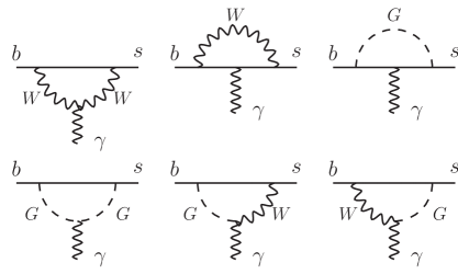
Figure 1: Leading order Feynman diagram of BXsγ𝐵subscript𝑋𝑠𝛾B\to X_{s}\gamma process.

In this subsection we focus attention on VLP contributions to rare B decay BXsγ𝐵subscript𝑋𝑠𝛾B\to X_{s}\gamma. The starting point for rare B decays is the determination of the low-energy effective Hamiltonian obtained by integrating out the heavy degrees of freedom in the theory. For bs𝑏𝑠b\to s transition, this can be written as

eff=GF2VtbVtsi=110[Ci(μ)Oi(μ)+Ci(μ)Oi(μ)],subscripteffsubscript𝐺𝐹2subscript𝑉𝑡𝑏superscriptsubscript𝑉𝑡𝑠superscriptsubscript𝑖110delimited-[]subscript𝐶𝑖𝜇subscript𝑂𝑖𝜇subscriptsuperscript𝐶𝑖𝜇subscriptsuperscript𝑂𝑖𝜇{\cal H}_{\rm eff}=-\frac{G_{F}}{\sqrt{2}}V_{tb}V_{ts}^{\ast}\sum_{i=1}^{10}[C_{i}(\mu)O_{i}(\mu)+C^{{}^{\prime}}_{i}(\mu)O^{{}^{\prime}}_{i}(\mu)]~{},~{}\, (109)

where the effective operators Oisubscript𝑂𝑖O_{i} are same as those in the SM defined in Ref. BLOSM . The chirality-flipped operators Oisubscriptsuperscript𝑂𝑖O^{\prime}_{i} are obtained from Oisubscript𝑂𝑖O_{i} by the replacement γ5γ5subscript𝛾5subscript𝛾5\gamma_{5}\to-\gamma_{5} in quark currentLi:2012xz . We calculate the Wilson coefficient C7subscript𝐶7C_{7} at matching scale mWsubscript𝑚𝑊m_{W}. The leading order Feynman diagrams are shown in FiG. 1 and C7subscript𝐶7C_{7} reads

C7(mW)subscript𝐶7subscript𝑚𝑊\displaystyle C_{7}(m_{W}) =\displaystyle= 1VtbVtsi=14[gLW(i,2)gLW(i,3)A(xi)+gLG(i,2)gLG(i,3)mui2xiB(xi)\displaystyle\frac{1}{V_{tb}V_{ts}^{\ast}}\sum_{i=1}^{4}\biggl{[}g_{L}^{W\ast}(i,2)g_{L}^{W}(i,3)A(x_{i})+\frac{g_{L}^{G\ast}(i,2)g_{L}^{G}(i,3)}{m_{u_{i}}^{2}}x_{i}B(x_{i}) (110)
+gLG(i,2)gRG(i,3)muimbxiC(xi)+gLW(i,2)gRG(i,3)mbD(xi)superscriptsubscript𝑔𝐿𝐺𝑖2superscriptsubscript𝑔𝑅𝐺𝑖3subscript𝑚subscript𝑢𝑖subscript𝑚𝑏subscript𝑥𝑖𝐶subscript𝑥𝑖superscriptsubscript𝑔𝐿𝑊𝑖2superscriptsubscript𝑔𝑅𝐺𝑖3subscript𝑚𝑏𝐷subscript𝑥𝑖\displaystyle+\frac{g_{L}^{G\ast}(i,2)g_{R}^{G}(i,3)}{m_{u_{i}}m_{b}}x_{i}C(x_{i})+\frac{g_{L}^{W\ast}(i,2)g_{R}^{G}(i,3)}{m_{b}}D(x_{i})
+muimbgLW(i,2)gRW(i,3)E(xi)+gLG(i,2)gRW(i,3)mbD(xi)]\displaystyle+\frac{m_{u_{i}}}{m_{b}}g_{L}^{W\ast}(i,2)g_{R}^{W}(i,3)E(x_{i})+\frac{g_{L}^{G\ast}(i,2)g_{R}^{W}(i,3)}{m_{b}}D(x_{i})\biggl{]}

where xi=mui2/mW2subscript𝑥𝑖superscriptsubscript𝑚subscript𝑢𝑖2superscriptsubscript𝑚𝑊2x_{i}=m_{u_{i}}^{2}/m_{W}^{2} and the loop function A(x),B(x),C(x),D(x),E(x)𝐴𝑥𝐵𝑥𝐶𝑥𝐷𝑥𝐸𝑥A(x),~{}B(x),~{}C(x),~{}D(x),~{}E(x) are listed in the appendix. The first two lines are the similar contribution as in the SM, while the last lines are the terms come form the tail terms. Note that the contribution of right diagram in the second line of FIG. 1 is zero in the SM. The terms with 1/mb1subscript𝑚𝑏1/m_{b} in above equation is extracted to compose the operator 𝒪7subscript𝒪7{\cal O}_{7}. There are two differences in the calculation of BXsγ𝐵subscript𝑋𝑠𝛾B\to X_{s}\gamma processes compared with the SM. One is the tail terms of gauge or Yukawa interactions, another one is the new type of Yukawa interactions listed in Eqs. (104, 105) which can not be written into the simple form in the SM such as

gLG,SM(i,2)=muiVis,gRG,SM(i,3)=mbVib.formulae-sequencesuperscriptsubscript𝑔𝐿𝐺SM𝑖2subscript𝑚subscript𝑢𝑖subscript𝑉𝑖𝑠superscriptsubscript𝑔𝑅𝐺SM𝑖3subscript𝑚𝑏subscript𝑉𝑖𝑏g_{L}^{G,\rm SM}(i,2)=m_{u_{i}}V_{is},~{}g_{R}^{G,\rm SM}(i,3)=-m_{b}V_{ib}. (111)
Table 2: The CKM matrix elements constrained by the tree-level B decays.
absolute value direct measurement from
Vudsubscript𝑉𝑢𝑑V_{ud} 0.97425±0.00022plus-or-minus0.974250.000220.97425\pm 0.00022 nuclear beta decay
Vussubscript𝑉𝑢𝑠V_{us} 0.2252±0.0009plus-or-minus0.22520.00090.2252\pm 0.0009 semi-leptonic K-decay
Vubsubscript𝑉𝑢𝑏V_{ub} 0.00415±0.00049plus-or-minus0.004150.000490.00415\pm 0.00049 semi-leptonic B-decay
Vcdsubscript𝑉𝑐𝑑V_{cd} 0.230±0.011plus-or-minus0.2300.0110.230\pm 0.011 semi-leptonic D-decay
Vcssubscript𝑉𝑐𝑠V_{cs} 1.006±0.023plus-or-minus1.0060.0231.006\pm 0.023 (semi-)leptonic D-decay
Vcbsubscript𝑉𝑐𝑏V_{cb} 0.0409±0.0011plus-or-minus0.04090.00110.0409\pm 0.0011 semi-leptonic B-decay
Vtbsubscript𝑉𝑡𝑏V_{tb} 0.89±0.07plus-or-minus0.890.070.89\pm 0.07 (single) top-production

In the model with three generation quarks, the CKM matrix unitarity is already used in the calculations of the loop-level FCNC induced rare B decays. For consistency, in numerical analysis the constraints on CKM matrix element are not from processes occurred at loop level, such as rare B decays, but from tree-level processes shown in Table 2 Beringer:1900zz ; Eberhardt:2010bm . Since there are no tree-level measurements of Vtdsubscript𝑉𝑡𝑑V_{td}, Vtssubscript𝑉𝑡𝑠V_{ts} now, we use above inputs and the unitarity to get 3×3333\times 3 unitary matrix at first. The method is that we scan (Vud,Vus,Vub)subscript𝑉𝑢𝑑subscript𝑉𝑢𝑠subscript𝑉𝑢𝑏(V_{ud},V_{us},V_{ub}) randomly (keeping |Vud|2+|Vus|2+|Vub|2=1superscriptsubscript𝑉𝑢𝑑2superscriptsubscript𝑉𝑢𝑠2superscriptsubscript𝑉𝑢𝑏21|V_{ud}|^{2}+|V_{us}|^{2}+|V_{ub}|^{2}=1 ) in range listed in Table 2, then we define two parameters α,β𝛼𝛽\alpha,~{}\beta and solve them by the equations

Vud(Vcd+α)+Vus(Vcs+β)+VubVcb=0,superscriptsubscript𝑉𝑢𝑑subscript𝑉𝑐𝑑𝛼superscriptsubscript𝑉𝑢𝑠subscript𝑉𝑐𝑠𝛽superscriptsubscript𝑉𝑢𝑏subscript𝑉𝑐𝑏0\displaystyle V_{ud}^{\ast}(V_{cd}+\alpha)+V_{us}^{\ast}(V_{cs}+\beta)+V_{ub}^{\ast}V_{cb}=0,
|Vcd+α|2+|Vcs+β|2+|Vcb|2=1.superscriptsubscript𝑉𝑐𝑑𝛼2superscriptsubscript𝑉𝑐𝑠𝛽2superscriptsubscript𝑉𝑐𝑏21\displaystyle\left|V_{cd}+\alpha\right|^{2}+\left|V_{cs}+\beta\right|^{2}+\left|V_{cb}\right|^{2}=1. (112)

(Vtd,Vts,Vtb)subscript𝑉𝑡𝑑subscript𝑉𝑡𝑠subscript𝑉𝑡𝑏(V_{td},V_{ts},V_{tb}) are got by the unitarity relation with (Vud,Vus,Vub)subscript𝑉𝑢𝑑subscript𝑉𝑢𝑠subscript𝑉𝑢𝑏(V_{ud},V_{us},V_{ub}) and (Vcd,Vcs,Vcb)subscript𝑉𝑐𝑑subscript𝑉𝑐𝑠subscript𝑉𝑐𝑏(V_{cd},V_{cs},V_{cb}). After that we times the 3×3333\times 3 unitary matrix with three matrices

(𝟏cosθ4isinθ4i𝟏sinθ4icosθ4i)1subscript𝜃4𝑖subscript𝜃4𝑖1subscript𝜃4𝑖subscript𝜃4𝑖\displaystyle\left(\begin{array}[]{cccc}{\bf 1}&\cdots&\cdots&\cdots\\ \cdots&\cos\theta_{4i}&\cdots&\sin\theta_{4i}\\ \cdots&\cdots&{\bf 1}&\cdots\\ \cdots&-\sin\theta_{4i}&\cdots&\cos\theta_{4i}\end{array}\right) (117)

in which i=1,2,3𝑖123i=1,~{}2,~{}3 and max(|θ41|,|θ42|,|θ43|)<0.01πsubscript𝜃41subscript𝜃42subscript𝜃430.01𝜋\max(|\theta_{41}|,~{}|\theta_{42}|,~{}|\theta_{43}|)<0.01\pi, to generate a 4×4444\times 4 unitary matrix UCKM4subscript𝑈CKM4U_{\rm CKM4}. VCKM4subscript𝑉CKM4V_{\rm CKM4} are got by the Eq. (108). All the corresponding elements should satisfy the experiment bound list in Table 2 and Vtdsubscript𝑉𝑡𝑑V_{td}, Vtssubscript𝑉𝑡𝑠V_{ts} (|Vts|0.04similar-to-or-equalssubscript𝑉𝑡𝑠0.04|V_{ts}|\simeq 0.04 which is consistent with the fitting results in Ref. Beringer:1900zz ) can be got too. With this inputs in hand, the first task is to check the scale of the mass parameter of model, such as MQsubscript𝑀𝑄M_{Q}, mX,mYsubscript𝑚𝑋subscript𝑚𝑌m_{X},m_{Y}. From the Zb¯b𝑍¯𝑏𝑏Z\bar{b}b vertexes in Eq. (106) and Eq. (107), we can see that in order to keep gauge universality of quarks, the tail terms in the Feynman rules must be much smaller than the SM like terms, namely |Zu,d4i|i=1,2,32,|Uu,d4i|i=1,2,32sin2θWmuch-less-thansubscriptsuperscriptsubscriptsuperscript𝑍4𝑖𝑢𝑑2𝑖123subscriptsuperscriptsubscriptsuperscript𝑈4𝑖𝑢𝑑2𝑖123superscript2subscript𝜃𝑊|Z^{4i}_{u,d}|^{2}_{i=1,2,3},~{}|U^{4i}_{u,d}|^{2}_{i=1,2,3}\ll\sin^{2}\theta_{W}. Thus in the numerical studies we require
Refer to caption
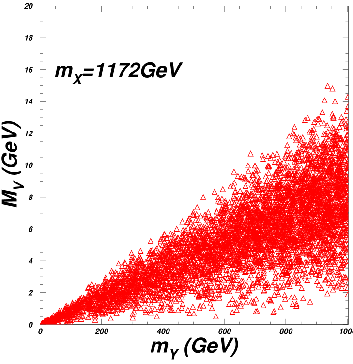
Figure 2: MVsubscript𝑀𝑉M_{V} versus MYsubscript𝑀𝑌M_{Y} under constraints |Zu,d4i|i=1,2,32,|Uu,d4i|i=1,2,32<104.subscriptsuperscriptsubscriptsuperscript𝑍4𝑖𝑢𝑑2𝑖123subscriptsuperscriptsubscriptsuperscript𝑈4𝑖𝑢𝑑2𝑖123superscript104|Z^{4i}_{u,d}|^{2}_{i=1,2,3},~{}|U^{4i}_{u,d}|^{2}_{i=1,2,3}<10^{-4}.
|Zu,d4i|i=1,2,32,|Uu,d4i|i=1,2,32<104.subscriptsuperscriptsubscriptsuperscript𝑍4𝑖𝑢𝑑2𝑖123subscriptsuperscriptsubscriptsuperscript𝑈4𝑖𝑢𝑑2𝑖123superscript104|Z^{4i}_{u,d}|^{2}_{i=1,2,3},~{}|U^{4i}_{u,d}|^{2}_{i=1,2,3}<10^{-4}. (118)

Note that though these elements are greater than λ3superscript𝜆3\lambda^{3} (parameter in the Wolfenstein parameterization Wolfenstein:1983yz ), they are much smaller than the product of VCKM3VCKM3superscriptsubscript𝑉CKM3subscript𝑉CKM3V_{\rm CKM3}^{\dagger}V_{\rm CKM3} (almost equals 𝟏1\bf 1), thus the requirements are suitable for indicating the contraints from the deviation from unitarity.

Since the scanning in the parameter space is freely, we set mX=1172GeVsubscript𝑚𝑋1172GeVm_{X}=1172{\rm GeV} (mass of top quark plus 1000 GeV) and scan mYsubscript𝑚𝑌m_{Y} in the range of (4.2,1004)GeV4.21004GeV(4.2,1004)\rm GeV (mass of bottom quark plus 1000 GeV), and Zu,d,Uu,dsubscript𝑍𝑢𝑑subscript𝑈𝑢𝑑Z_{u,d},~{}U_{u,d} randomly (ignoring the CP phases). MVsubscript𝑀𝑉M_{V} is defined by

MV=max(|MQ1|,|MQ2|,|MQ3|).subscript𝑀𝑉superscriptsubscript𝑀𝑄1superscriptsubscript𝑀𝑄2superscriptsubscript𝑀𝑄3M_{V}=\max(|M_{Q}^{1}|,~{}|M_{Q}^{2}|,~{}|M_{Q}^{3}|). (119)

The result for MVsubscript𝑀𝑉M_{V} versus MYsubscript𝑀𝑌M_{Y} is shown in the FIG. 2 which checks the mass input of vector doublet. We can see that MVsubscript𝑀𝑉M_{V} increases as mYsubscript𝑚𝑌m_{Y} growing up. However MVsubscript𝑀𝑉M_{V} is much smaller than mXsubscript𝑚𝑋m_{X} and mYsubscript𝑚𝑌m_{Y}. Small mixings lead to parameter MQsubscript𝑀𝑄M_{Q} which determine the mixing between SM quarks and vector like quarks are also suppressed. This is in agreement with that the deviation from unitarity is suppressed by the ratio m/mX,Y𝑚subscript𝑚𝑋𝑌m/m_{X,Y} where m𝑚m denotes generically the standard quark masses, which is a typical result of VLP models. Langacker:1988ur ; delAguila:1982fs ; delAguila:1987nn ; Cheng:1991rr ; Botella:2012ju
Refer to caption
Refer to caption
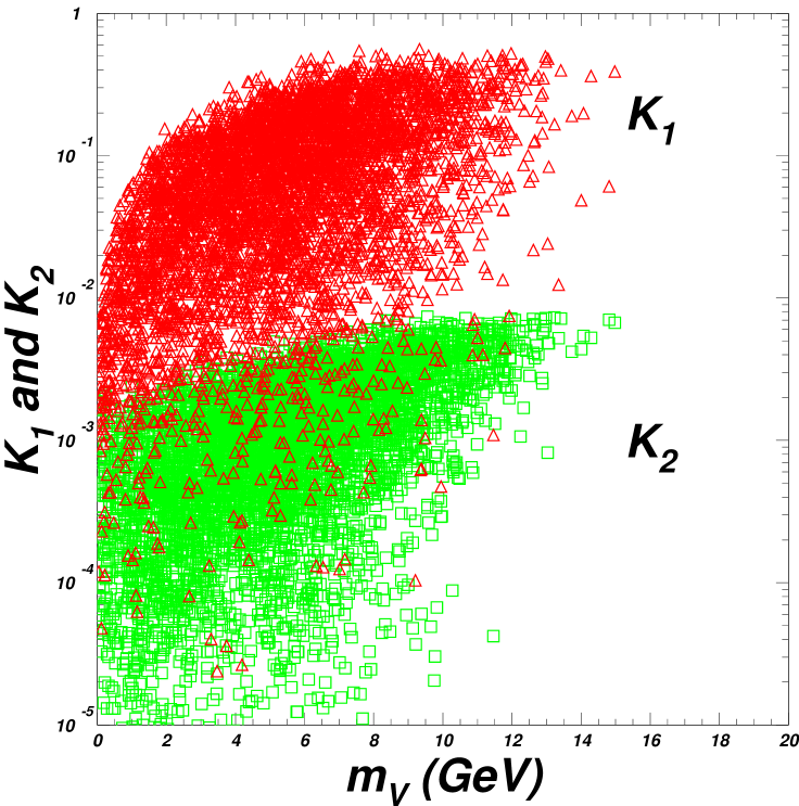
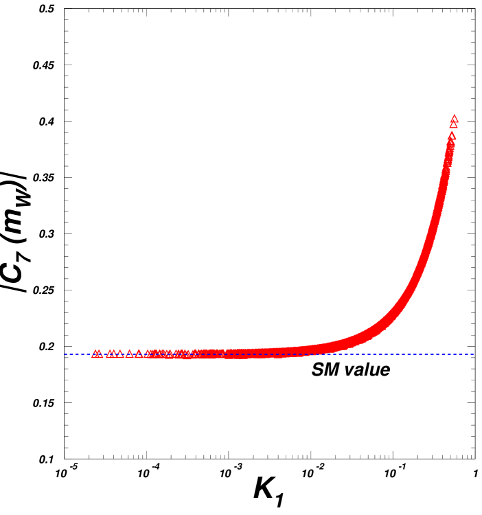
Figure 3: K1subscript𝐾1K_{1}, (red \triangle) K2subscript𝐾2K_{2} (green \Box) versus MVsubscript𝑀𝑉M_{V} and enhancement of |C7(mW)|subscript𝐶7subscript𝑚𝑊|C_{7}(m_{W})| case of |Zu,d4i|i=1,2,32,|Uu,d4i|i=1,2,32<104subscriptsuperscriptsubscriptsuperscript𝑍4𝑖𝑢𝑑2𝑖123subscriptsuperscriptsubscriptsuperscript𝑈4𝑖𝑢𝑑2𝑖123superscript104|Z^{4i}_{u,d}|^{2}_{i=1,2,3},~{}|U^{4i}_{u,d}|^{2}_{i=1,2,3}<10^{-4} (color online).

The second task is to check the VLP contribution to BXsγ𝐵subscript𝑋𝑠𝛾B\to X_{s}\gamma. We find the Wilson coefficient of FCNC operator O7subscript𝑂7O_{7} is not so suppressed as the mixing. The new contributions, from the terms of the last line in Eq.(110) are suppressed by the mixing, whereas the terms of first line are almost the same as the SM. The enhancement comes mainly from the gRG(4,3)/mbsuperscriptsubscript𝑔𝑅𝐺43subscript𝑚𝑏g_{R}^{G}(4,3)/m_{b} terms which are got from the Goldstone loop in bs𝑏𝑠b\to s transition. (The right diagram in the first line and diagrams in the second line of the Fig. 1) In order to show the enhancement clearly, we define two factors

K1subscript𝐾1\displaystyle K_{1} =\displaystyle= gRG(4,3)gLG(4,2)mXmbVtbVts=gRGVbgLGVsmXmbVtbVts,superscriptsubscript𝑔𝑅𝐺43superscriptsubscript𝑔𝐿𝐺superscript42subscript𝑚𝑋subscript𝑚𝑏subscript𝑉𝑡𝑏superscriptsubscript𝑉𝑡𝑠superscriptsubscript𝑔𝑅𝐺𝑉𝑏superscriptsubscript𝑔𝐿𝐺𝑉𝑠subscript𝑚𝑋subscript𝑚𝑏subscript𝑉𝑡𝑏superscriptsubscript𝑉𝑡𝑠\displaystyle\frac{g_{R}^{G}(4,3)g_{L}^{G}(4,2)^{\ast}}{m_{X}m_{b}V_{tb}V_{ts}^{\ast}}=\frac{g_{R}^{GVb}g_{L}^{GVs\ast}}{m_{X}m_{b}V_{tb}V_{ts}^{\ast}}\,, (120)
K2subscript𝐾2\displaystyle K_{2} =\displaystyle= U43U42VtbVts=UVbUVsVtbVts,superscript𝑈43superscript𝑈42subscript𝑉𝑡𝑏superscriptsubscript𝑉𝑡𝑠superscript𝑈𝑉𝑏superscript𝑈𝑉𝑠subscript𝑉𝑡𝑏superscriptsubscript𝑉𝑡𝑠\displaystyle\frac{U^{43}U^{42\ast}}{V_{tb}V_{ts}^{\ast}}=\frac{U^{Vb}U^{Vs\ast}}{V_{tb}V_{ts}^{\ast}}\,, (121)

in which K2subscript𝐾2K_{2} denotes the deviation from the unitarity of 3×3333\times 3 CKM matrix, while K1subscript𝐾1K_{1} shows the enhancement of the contribution from vector like particles. K1subscript𝐾1K_{1} is in fact got from the coefficient of first term in the second line of analytical expression of C7(mW)subscript𝐶7subscript𝑚𝑊C_{7}(m_{W}) in Eq. (110) when i=4𝑖4i=4. It will be changed into exactly K2subscript𝐾2K_{2} in case of the SM4. Note that other terms with gRG(4,3)/mbsuperscriptsubscript𝑔𝑅𝐺43subscript𝑚𝑏g_{R}^{G}(4,3)/m_{b} can give enhancement too, we chose factor K1subscript𝐾1K_{1} for a typical demonstration since it seems that it will be suppressed by mXsubscript𝑚𝑋m_{X}. Results are shown in the FIG 3 in which the left panel shows K1subscript𝐾1K_{1} and K2subscript𝐾2K_{2} versus MVsubscript𝑀𝑉M_{V} while the right panel shows |C7(mW)|subscript𝐶7subscript𝑚𝑊|C_{7}(m_{W})| versus K1subscript𝐾1K_{1}. From the left panel, we can see that though K2subscript𝐾2K_{2} increase as MVsubscript𝑀𝑉M_{V} increases, it is still much smaller than VtbVtssubscript𝑉𝑡𝑏superscriptsubscript𝑉𝑡𝑠V_{tb}V_{ts}^{\ast}, implying that deviation of unitarity are negligible. However the factor K1subscript𝐾1K_{1} can be enhanced up to order 𝒪(1)𝒪1{\cal O}(1) by the increase of MVsubscript𝑀𝑉M_{V}. From the right panel, we can see that K1subscript𝐾1K_{1} enhances C7subscript𝐶7C_{7} up to a value much larger that the result of the SM. The reason for the enhancement mainly comes from the new type of Yukawa couplings. Combining of Eqs. (99104105), one can get similar form compared with the SM4

gLG(4,2)mXsubscriptsuperscript𝑔𝐺𝐿42subscript𝑚𝑋\displaystyle\frac{g^{G}_{L}(4,2)}{m_{X}} =\displaystyle= UCKM442+1mX[m=13(MQmUdm2Zu44MumUd42Zum4)+(YVdYVu)Ud42Zu44v],superscriptsubscript𝑈𝐶𝐾𝑀4421subscript𝑚𝑋delimited-[]superscriptsubscript𝑚13superscriptsubscript𝑀𝑄𝑚superscriptsubscript𝑈𝑑𝑚2superscriptsubscript𝑍𝑢absent44superscriptsubscript𝑀𝑢𝑚superscriptsubscript𝑈𝑑42superscriptsubscript𝑍𝑢absent𝑚4subscript𝑌𝑉𝑑subscript𝑌𝑉𝑢superscriptsubscript𝑈𝑑42superscriptsubscript𝑍𝑢absent44𝑣\displaystyle U_{CKM4}^{42}+\frac{1}{m_{X}}\left[\sum_{m=1}^{3}\left(M_{Q}^{m}U_{d}^{m2}Z_{u}^{\ast 44}-M_{u}^{m}U_{d}^{42}Z_{u}^{\ast m4}\right)+(Y_{Vd}-Y_{Vu})U_{d}^{42}Z_{u}^{\ast 44}v\right], (122)
gRG(4,3)mbsubscriptsuperscript𝑔𝐺𝑅43subscript𝑚𝑏\displaystyle\frac{g^{G}_{R}(4,3)}{m_{b}} =\displaystyle= UCKM4431mb[m=13(MQmUum4Zd43+MdmUu44Zdm3)+(YVdYVu)Uu44Zd43v].superscriptsubscript𝑈𝐶𝐾𝑀4absent431subscript𝑚𝑏delimited-[]superscriptsubscript𝑚13superscriptsubscript𝑀𝑄absent𝑚superscriptsubscript𝑈𝑢absent𝑚4superscriptsubscript𝑍𝑑43superscriptsubscript𝑀𝑑absent𝑚superscriptsubscript𝑈𝑢absent44superscriptsubscript𝑍𝑑𝑚3subscriptsuperscript𝑌𝑉𝑑superscriptsubscript𝑌𝑉𝑢superscriptsubscript𝑈𝑢absent44superscriptsubscript𝑍𝑑43𝑣\displaystyle-U_{CKM4}^{\ast 43}-\frac{1}{m_{b}}\left[\sum_{m=1}^{3}\left(M_{Q}^{\ast m}U_{u}^{\ast m4}Z_{d}^{43}+M_{d}^{\ast m}U_{u}^{\ast 44}Z_{d}^{m3}\right)+(Y^{*}_{Vd}-Y_{Vu}^{\ast})U_{u}^{\ast 44}Z_{d}^{43}v\right]. (123)

Since mXYVuvsimilar-to-or-equalssubscript𝑚𝑋subscript𝑌𝑉𝑢𝑣m_{X}\simeq Y_{Vu}v, Zu44,Uu441similar-to-or-equalssuperscriptsubscript𝑍𝑢44superscriptsubscript𝑈𝑢441Z_{u}^{44},~{}U_{u}^{44}\simeq 1, one can easily obtain that

gLG(4,2)mXVCKM442,similar-tosubscriptsuperscript𝑔𝐺𝐿42subscript𝑚𝑋superscriptsubscript𝑉CKM442\frac{g^{G}_{L}(4,2)}{m_{X}}\sim V_{\rm CKM4}^{42}, (124)

the suppression of Zd43superscriptsubscript𝑍𝑑43Z_{d}^{43} (order of m/mX,Y𝑚subscript𝑚𝑋𝑌m/m_{X,Y}) in Eq. (123) are enhanced by terms with factor such as YVuvmbsubscript𝑌𝑉𝑢𝑣subscript𝑚𝑏\frac{Y_{Vu}v}{m_{b}}, etc., resulting

gRG(4,3)mbVCKM443.much-greater-thansubscriptsuperscript𝑔𝐺𝑅43subscript𝑚𝑏superscriptsubscript𝑉CKM443\frac{g^{G}_{R}(4,3)}{m_{b}}\gg V_{\rm CKM4}^{43}. (125)

Thus the term V4bV4ssubscript𝑉4𝑏superscriptsubscript𝑉4𝑠V_{4b}V_{4s}^{\ast} satisfying the unitary constraint

VubVus+VcbVcs+VtbVts+V4bV4s=0subscript𝑉𝑢𝑏superscriptsubscript𝑉𝑢𝑠subscript𝑉𝑐𝑏superscriptsubscript𝑉𝑐𝑠subscript𝑉𝑡𝑏superscriptsubscript𝑉𝑡𝑠subscript𝑉4𝑏superscriptsubscript𝑉4𝑠0V_{ub}V_{us}^{\ast}+V_{cb}V_{cs}^{\ast}+V_{tb}V_{ts}^{\ast}+V_{4b}V_{4s}^{\ast}=0 (126)

is enhanced greatly by heavy VLPs, then the factor leads the enhancement to C7subscript𝐶7C_{7}. This is different from those in the SM4 in which the contribution from the fourth generation can be neglected.
Refer to caption
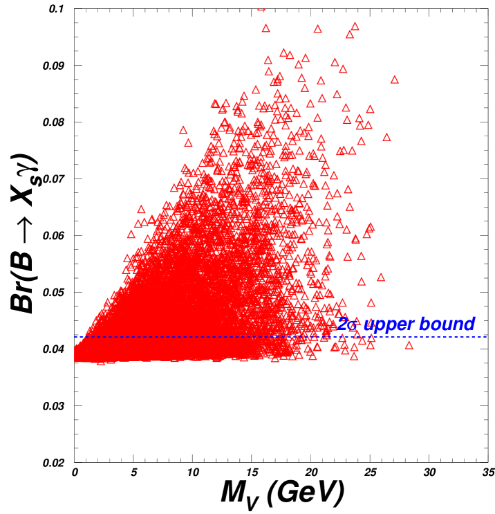
Figure 4: BXsγ𝐵subscript𝑋𝑠𝛾B\to X_{s}\gamma prediction in random scan.

In the numerical scan, we vary Zu,dsubscript𝑍𝑢𝑑Z_{u,d} and Uu,dsubscript𝑈𝑢𝑑U_{u,d} randomly, keeping the constraints of |Vu,d4i|i=1,2,32,|Uu,d4i|i=1,2,32subscriptsuperscriptsubscriptsuperscript𝑉4𝑖𝑢𝑑2𝑖123subscriptsuperscriptsubscriptsuperscript𝑈4𝑖𝑢𝑑2𝑖123|V^{4i}_{u,d}|^{2}_{i=1,2,3},~{}|U^{4i}_{u,d}|^{2}_{i=1,2,3}, scan mXsubscript𝑚𝑋m_{X} and mYsubscript𝑚𝑌m_{Y} in the range of (1,2000)GeV12000GeV(1,2000)\rm GeV. Apart from the CKM limits, we use the BXsγ𝐵subscript𝑋𝑠𝛾B\to X_{s}\gamma process to constrain parameter space. The branching ratio of BXsγ𝐵subscript𝑋𝑠𝛾B\to X_{s}\gamma is normalized by the process BXceνe¯𝐵subscript𝑋𝑐𝑒¯subscript𝜈𝑒B\rightarrow X_{c}e\bar{\nu_{e}}:

Br(BXsγ)=Brex(BXceνe¯)|VtsVtb|2|Vcb|26απf(z)[|C7eff(μb)|2+|C7,eff(μb)|2].Br𝐵subscript𝑋𝑠𝛾superscriptBrex𝐵subscript𝑋𝑐𝑒¯subscript𝜈𝑒superscriptsuperscriptsubscript𝑉𝑡𝑠subscript𝑉𝑡𝑏2superscriptsubscript𝑉𝑐𝑏26𝛼𝜋𝑓𝑧delimited-[]superscriptsubscriptsuperscript𝐶eff7subscript𝜇𝑏2superscriptsubscriptsuperscript𝐶eff7subscript𝜇𝑏2{\rm Br}(B\rightarrow X_{s}\gamma)={\rm Br}^{\rm ex}(B\rightarrow X_{c}e\bar{\nu_{e}})\frac{|V_{ts}^{\ast}V_{tb}|^{2}}{|V_{cb}|^{2}}\frac{6\alpha}{\pi f(z)}[|C^{\rm eff}_{7}(\mu_{b})|^{2}+|C^{\prime,\rm eff}_{7}(\mu_{b})|^{2}]. (127)

Here z=mcmb𝑧subscript𝑚𝑐subscript𝑚𝑏z=\frac{m_{c}}{m_{b}}, and f(z)=18z2+8z6z824z4lnz𝑓𝑧18superscript𝑧28superscript𝑧6superscript𝑧824superscript𝑧4𝑧f(z)=1-8z^{2}+8z^{6}-z^{8}-24z^{4}\ln z is the phase-space factor in the semi-leptonic B decay. The method of running of the operators from mWsubscript𝑚𝑊m_{W} scale to μbsubscript𝜇𝑏\mu_{b} scale can be found in Ref. Li:2012xz . We use the following bounds on the calculation Beringer:1900zz

Brex(bceν¯e)=(10.72±0.13)×102,superscriptBrex𝑏𝑐𝑒subscript¯𝜈𝑒plus-or-minus10.720.13superscript102\displaystyle{\rm Br}^{\rm ex}(b\to ce\overline{\nu}_{e})=(10.72\pm 0.13)\times 10^{-2}, (128)
Brex(BXsγ)=(3.55±0.24±0.09)×104.superscriptBrex𝐵subscript𝑋𝑠𝛾plus-or-minus3.550.240.09superscript104\displaystyle{\rm Br}^{\rm ex}(B\to X_{s}\gamma)=(3.55\pm 0.24\pm 0.09)\times 10^{-4}. (129)

The numerical results show that the C7,eff(μb)subscriptsuperscript𝐶eff7subscript𝜇𝑏C^{\prime,\rm eff}_{7}(\mu_{b}) is much smaller than C7eff(μb)subscriptsuperscript𝐶eff7subscript𝜇𝑏C^{\rm eff}_{7}(\mu_{b}), therefore we do not present the formula of C7,eff(mW)subscriptsuperscript𝐶eff7subscript𝑚𝑊C^{\prime,\rm eff}_{7}(m_{W}) here.

The branching ratio as a function of mVsubscript𝑚𝑉m_{V} is shown in FIG. 4, from which we can see that Br(BXsγ)Br𝐵subscript𝑋𝑠𝛾{\rm Br}({B}\to X_{s}\gamma) can be enhanced much greater than the experiment bound. Then the measurements of FCNC process can give a stringent constraint on the vector like quark model, especially when the masses of vector quark are much greater than the electro-weak scale. A few remarks should be addressed:

  • There is one point of view on the unitarity of the CKM matrix which is that the 3×3333\times 3 ordinary quark mixing matrix is regarded as nearly unitary, deviation from unitarity is suppressed by heavy particle in the new physics beyond the SM. In other word, one admits that the extended CKM matrix elements exist, they approach to zero while mass scale of the new physics approaches to infinity. All the new physical effects should decouple from the flavor sector and what should be checked is that if 3×3333\times 3 unitariry is consistent in all kinds of flavor processes.

  • Another point of view is that, as in the SM case, the 3×3333\times 3 ordinary quark mixing matrix elements are only extracted by experiments in the measurements of tree and loop level precesses. The unitarity should be checked, experiment measurements on the elements of matrix can be used as the constraints to the new physics beyond the SM. In the numerical analysis, the elements of CKM matrix are regarded as inputs. Thus what should be done is to scan the parameter space generally under these constraints, no prejudice should be imposed. Then the enhancement effect in BXsγ𝐵subscript𝑋𝑠𝛾B\to X_{s}\gamma will be more clear.

Refer to caption
Refer to caption
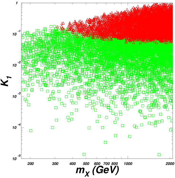
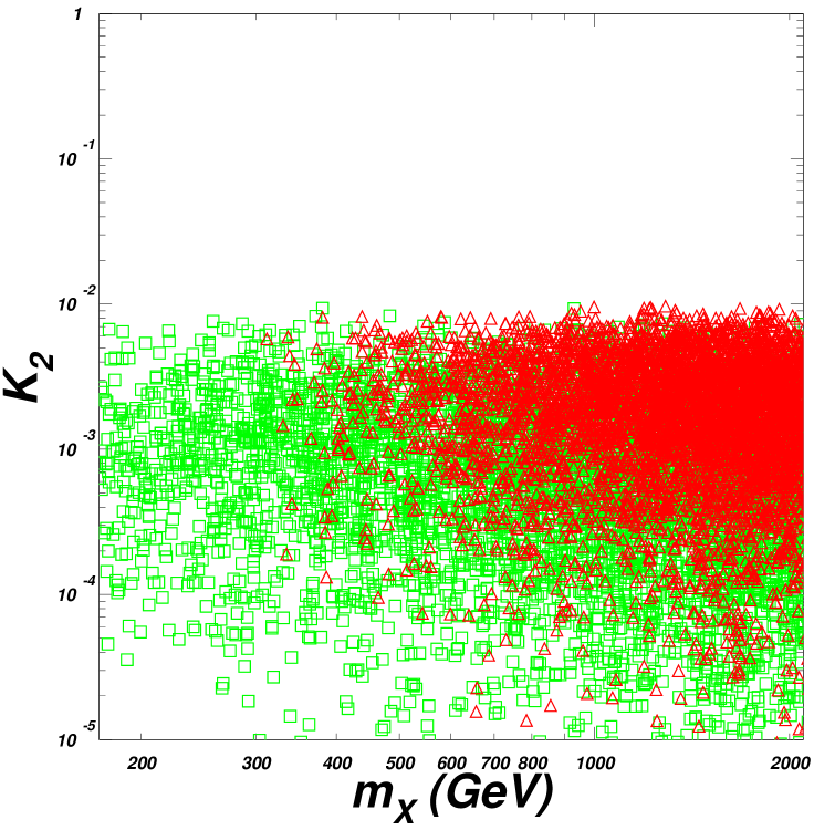
Figure 5: Enhancement factor and deviation from unitarity versus mXsubscript𝑚𝑋m_{X}, red \triangle are excluded by the bound of BXsγ𝐵subscript𝑋𝑠𝛾B\to X_{s}\gamma measurement which the green \Box are the survived points (color online).

Large parameter space is excluded by the measured branching fraction of BXsγ𝐵subscript𝑋𝑠𝛾B\to X_{s}\gamma as shown in FIG. 4. The enhancement effect of the VLPs can be seen in FIG. 5 in which the left panel shows the enhancement factor K1subscript𝐾1K_{1} versus mXsubscript𝑚𝑋m_{X} while the right panel shows K2subscript𝐾2K_{2} versus mXsubscript𝑚𝑋m_{X}. From the right panel we can see that deviation from unitarity are very small and almost irrelevant with mXsubscript𝑚𝑋m_{X} since we are doing a general scan of Zu,dsubscript𝑍𝑢𝑑Z_{u,d} and Uu,dsubscript𝑈𝑢𝑑U_{u,d}. However as we see from the left panel, as mXsubscript𝑚𝑋m_{X} increases up, Br(BXsγ)Br𝐵subscript𝑋𝑠𝛾{\rm Br}({B}\to X_{s}\gamma) measurement will constrain the enhancement factor and then constrain the input parameter of mXsubscript𝑚𝑋m_{X}. In all, the enhancement can be summarized as that when mass of vector like particle increases up, it will increase the mass parameter mVsubscript𝑚𝑉m_{V} thus give an enhancement factor under very small deviation from unitarity. This should be a special point when we do the study on the vector like quark models.

IV Summary

In the model with vector doublets, there exist bilinear terms in the lagrangian, making the general scan of the Yukawa coupling very difficult. In this paper, we show a trick to deal with the scan. Our scan method are exactly and the more efficient. We use the trick to study a very simple extension of the SM with vector like quarks. We studied one of the most important rare B decay BXsγ𝐵subscript𝑋𝑠𝛾B\to X_{s}\gamma process in which we found that even the deviations from the unitarity of quark mixing matrix are small, the enhancement to rare B decay from VLPs are still significant. The enhanced effect is an important feature in the vector like particle model. In this work we just show the scan method, the key point of the enhancement and how stringent constraints on the parameter space from BXsγ𝐵subscript𝑋𝑠𝛾B\to X_{s}\gamma measurements. What should be done includes models like extension of the SM with VLPs, two higgs doublets models Grinstein:1990tj or supersymmetry models Altmannshofer:2009ne . Such effect should be checked in all kinds of rare decays such as inclusive process bs+𝑏𝑠superscriptsuperscriptb\to s\ell^{+}\ell^{-} and exclusive processes Bsμ+μsubscript𝐵𝑠superscript𝜇superscript𝜇B_{s}\to\mu^{+}\mu^{-}, Bs+γsubscript𝐵𝑠superscriptsuperscript𝛾B_{s}\to\ell^{+}\ell^{-}\gamma and BB¯𝐵¯𝐵B\bar{B} mixing et. al. The detailed studies on the parameter space including other rare B decays and new models will appear in our future work.

Acknowledgements.
This work was supported by the Natural Science Foundation of China under grant numbers 11375001 and by talents foundation of education department of Beijing.

Appendix

  • The loop functions for calculating the Wilson coefficients at the matching scale are the following

A(x)𝐴𝑥\displaystyle A(x) =\displaystyle= 55170x+127x236(1x)3+4x17x2+15x36(1x)4lnx,55170𝑥127superscript𝑥236superscript1𝑥34𝑥17superscript𝑥215superscript𝑥36superscript1𝑥4𝑥\displaystyle\frac{55-170x+127x^{2}}{36(1-x)^{3}}+\frac{4x-17x^{2}+15x^{3}}{6(1-x)^{4}}\ln x,
B(x)𝐵𝑥\displaystyle B(x) =\displaystyle= 7+5x+8x236(1x)3+2x+3x26(1x)4lnx,75𝑥8superscript𝑥236superscript1𝑥32𝑥3superscript𝑥26superscript1𝑥4𝑥\displaystyle\frac{-7+5x+8x^{2}}{36(1-x)^{3}}+\frac{-2x+3x^{2}}{6(1-x)^{4}}\ln x,
C(x)𝐶𝑥\displaystyle C(x) =\displaystyle= 35x6(1x)2+23x3(1x)3lnx,35𝑥6superscript1𝑥223𝑥3superscript1𝑥3𝑥\displaystyle\frac{3-5x}{6(1-x)^{2}}+\frac{2-3x}{3(1-x)^{3}}\ln x,
D(x)𝐷𝑥\displaystyle D(x) =\displaystyle= 3x14(1x)2+x22(1x)3lnx,3𝑥14superscript1𝑥2superscript𝑥22superscript1𝑥3𝑥\displaystyle\frac{3x-1}{4(1-x)^{2}}+\frac{x^{2}}{2(1-x)^{3}}\ln x,
E(x)𝐸𝑥\displaystyle E(x) =\displaystyle= 17+19x6(1x)2+8x+9x23(1x)3lnx.1719𝑥6superscript1𝑥28𝑥9superscript𝑥23superscript1𝑥3𝑥\displaystyle\frac{-17+19x}{6(1-x)^{2}}+\frac{-8x+9x^{2}}{3(1-x)^{3}}\ln x.

References

  • (1) G. Cvetic, Rev. Mod. Phys.  71, 513 (1999) [hep-ph/9702381]; H. J. He, T. M. P. Tait and C. P. Yuan, Phys. Rev. D 62, 011702 (2000) [hep-ph/9911266]; H. J. He, C. T. Hill and T. M. P. Tait, Phys. Rev. D 65, 055006 (2002) [hep-ph/0108041]. J. Cao, L. Shang, W. Su, F. Wang and Y. Zhang, arXiv:1512.08392 [hep-ph]. F. Wang, W. Wang, L. Wu, J. M. Yang and M. Zhang, arXiv:1512.08434 [hep-ph].
  • (2) J. Jiang, T. Li, D. V. Nanopoulos and D. Xie, Phys. Lett.  B 677, 322 (2009); Nucl. Phys.  B 830, 195 (2010).
  • (3) J. Jiang, T. Li and D. V. Nanopoulos, Nucl. Phys.  B 772, 49 (2007).
  • (4) I. Antoniadis, J. R. Ellis, J. S. Hagelin and D. V. Nanopoulos, Phys. Lett.  B 208, 209 (1988) [Addendum-ibid.  B 213, 562 (1988)]; Phys. Lett.  B 231, 65 (1989).
  • (5) J. L. Lopez, D. V. Nanopoulos and K. J. Yuan, Nucl. Phys.  B 399, 654 (1993).
  • (6) C. Beasley, J. J. Heckman and C. Vafa, JHEP 0901, 058 (2009); JHEP 0901, 059 (2009); R. Donagi and M. Wijnholt, Adv. Theor. Math. Phys.  15, no. 5, 1237 (2011) [arXiv:0802.2969 [hep-th]]; Adv. Theor. Math. Phys.  15, no. 6, 1523 (2011) [arXiv:0808.2223 [hep-th]].
  • (7) T. Li, D. V. Nanopoulos, W. Y. Wang, X. C. Wang and Z. H. Xiong, JHEP 1207, 190 (2012) [arXiv:1204.5326 [hep-ph]].
  • (8) T. Li, W. Wang, X. C. Wang and Z. H. Xiong, arXiv:1506.04987 [hep-ph].
  • (9) A. J. Buras, M. Misiak, M. Münz and S. Pokorski, Nucl. Phys. B 424, 374 (1994).
  • (10) J. Beringer et al. [Particle Data Group Collaboration], Phys. Rev. D 86, 010001 (2012).
  • (11) O. Eberhardt, A. Lenz and J. Rohrwild, Phys. Rev. D 82, 095006 (2010) [arXiv:1005.3505 [hep-ph]].
  • (12) L. Wolfenstein, Phys. Rev. Lett.  51, 1945 (1983). A. J. Buras, M. E. Lautenbacher and G. Ostermaier, Phys. Rev. D 50, 3433 (1994) [hep-ph/9403384]. J. Charles et al. [CKMfitter Group Collaboration], Eur. Phys. J. C 41, 1 (2005) [hep-ph/0406184].
  • (13) P. Langacker and D. London, Phys. Rev. D38 (1988) 886.
  • (14) F. del Aguila and M. Bowick, Nucl. Phys. B224 (1983) 107.
  • (15) F. del Aguila, E. Laermann, and P. Zerwas, Nucl. Phys. B297 (1988) 1.
  • (16) T. Cheng and L.-F. Li, Phys. Rev. D45 (1992) 1708–1710.
  • (17) F. J. Botella, G. C. Branco and M. Nebot, JHEP 1212, 040 (2012) [arXiv:1207.4440 [hep-ph]]; A. K. Alok, S. Banerjee, D. Kumar, S. U. Sankar and D. London, Phys. Rev. D 92, no. 1, 013002 (2015) [arXiv:1504.00517 [hep-ph]]; A. K. Alok, S. Banerjee, D. Kumar and S. Uma Sankar, Nucl. Phys. B 906, 321 (2016) [arXiv:1402.1023 [hep-ph]].
  • (18) B. Grinstein, R. P. Springer and M. B. Wise, Nucl. Phys. B 339, 269 (1990).
  • (19) W. Altmannshofer, A. J. Buras, S. Gori, P. Paradisi and D. M. Straub, Nucl. Phys. B 830, 17 (2010) [arXiv:0909.1333 [hep-ph]].