Atomic orientation by a broadly frequency-modulated radiation: theory and experiment.

Abstract

We investigate magnetic resonances driven in thermal vapour of alkali atoms by laser radiation broadly modulated at a frequency resonant with the Zeeman splitting. A model accounting for both hyperfine and Zeeman pumping is developed and its results are compared with experimental measurements performed at relatively weak pump irradiance. The interplay between the two pumping processes generates intriguing interaction conditions, often overlooked by simplified models.

I Introduction

Optical pumping processes in atomic samples William Happer et al. (2010) have been subject of intensive theoretical and experimental studies since the 60s Happer (1972), and have been used in several applications including, laser cooling Metcalf and van der Straten (1999), molecular spectroscopy abd Ruvin Ferber (2005) and atomic magnetometry. Atomic magnetometers are nowadays available as commercial devices, but further research is presently carried out to optimize the performance, as well as to better understand phenomena and mechanisms which subtly act in this kind of apparatuses.

The interest in precise and sensitive magnetic field measurements led to a revival of the research in magnetometry, and particularly in the optical-atomic sensors. Optical magnetometers were recently subject to impressive advances in terms of sensitivity. The possibility of absolute field measurements, the low operation costs and power consumption, the robustness, and the potential for miniaturization, let these devices compete with superconducting quantum interference devices, traditionally regarded as state-of-the-art magnetometric sensors.

The typical working principle of an atomic optical magnetometer Aleksandrov and Vershovskii (2009) is based on the preparation of an atomic state using optical pumping and on the detection of its time-evolution driven by the magnetic field under measurement. Some recent works on atomic magnetometry have addressed time-domain operation techniques, where the atomic state is first prepared and then is followed in its free evolution within the decay time Lenci et al. (2014). In contrast, most of the approaches reported in the literature are based on a frequency-domain detection Budker and Romalis (2007). In this case, a steady-state condition is reached, by means of a periodic regeneration of the atomic state to be analyzed. This regeneration is obtained by applying an appropriate optical radiation having some parameter periodically modulated in resonance (or near-resonance) with the evolution of the atomic state. Experiments have been reported where the modulated parameter of the pump radiation is its amplitude Suter and Mlynek (1991); Schultze et al. (2012); Rosatzin et al. (1990), its polarization Klepel and Suter (1992); Breschi et al. (2013, 2014); Bevilacqua and Breschi (2014), or its optical frequency Belfi et al. (2007); Acosta et al. (2006). Different macroscopic quantities have been chosen to be measured as well, such as the absorption Breschi et al. (2013), the polarization rotation Zigdon et al. (2010); Bevilacqua et al. (2012); Sheng et al. (2013), or (in similar experiments based on solid-state samples) the fluorescence Wolf et al. (2015), all opening an indirect way to follow the vapour magnetization.

Optical pumping is often applied in regime of strong intensity where power broadening and non linear dependence on the laser intensity occur. Studies in low intensity regime are also reported Sydoryk et al. (2008).

Our study concerns a setup developed for precise atomic magnetometry, which here is operated in a condition of weak excitation intensity. The atomic sample is illuminated by two collinear laser beams. One of them (modulated beam, MB in the following) is frequency modulated and circularly polarized, and the second one (detection beam, DB) is linearly polarized with polarization plane rotated by the time dependent circular birefringence of the sample. In other terms, the MB induces a magnetic dipole that precesses at the Larmor frequency and the dipole component parallel to the beams is monitored.

The MB is broadly modulated in frequency, thus both the ground hyperfine states of the atomic vapour are excited with non-vanishing rates. Such broad modulation gives rise to an important interplay between hyperfine and Zeeman pumping that takes advantages in optical magnetometry Bevilacqua et al. (2016a). The proposed excitation scheme not only simplifies the setup (pump-repump scheme is often applied as an alternative), but has the potential of significantly increasing the signal without increasing the magnetic resonances width, particularly at higher intensities, with obvious practical implications.

In this work we address mainly the aspects related to the wide MB frequency modulation, restricting the investigation to a regime of relatively weak intensity, deferring the analysis of the intense pumping to another study. We develop a model considering the MB interaction with the whole level structure of the $D_{1}$ Cs transitions: a point which is often overlooked in the literature. We obtain a modified version of the Larmor equation for the magnetization created in a given ground state Zeeman multiplet. An analytical expression for the magnetization amplitude, pointing out the dependence on the MB modulation parameters, is found and it matches very well with the experiment.

The paper is organized as follows: in Section II we briefly describe the experimental apparatus; in Section III the theoretical model is reported; finally in Section IV we discuss and compare the theoretical and the experimental results.

II Experimental setup

A detailed description of the experimental set-up is given in Refs.Bevilacqua et al. (2012); Bevilacqua et al. (2016a). Briefly, Cs vapour is contained in a sealed cell, where buffer gas is added to counteract time-of-flight line broadening of the magnetic resonances and to increase the optical pumping effect. The Cs Atoms are optically pumped by a circularly polarized, near resonant laser (MB) light at 894 nm ($D_{1}$ Cs line). The cell is at room temperature and in a highly homogeneous magnetic field. A balanced polarimeter enables the detection of the atomic precession, which causes the polarization rotation of a linearly polarized beam (DB), near resonant with the $F_{g}$ = 4 to $F_{e}$ = 3, 4, 5 group of transitions belonging to the Cs $D_{2}$ line. The set-up contains two channels (see Fig. 1), which in magnetometric applications Bevilacqua et al. (2009, 2013); Bevilacqua et al. (2016b) are used to reject common-mode magnetic noise and to measure local magnetic variations by means of a differential method. In the present work one of the channels keeps being used to detect the atomic spins precession, while the other one (monitor, MNT) is used for precise determination of the DB and MB intensities and absolute frequencies. The DB radiation is attenuated down to 10 nano-Watt and kept at a constant frequency, blue detuned by about 2 GHz with respect to the D₂ transition set starting from $F_{g}=4$. The MB radiation, which in magnetometric applications was in the milli-Watt range, here is attenuated down to 100 nano-Watt and its optical frequency is made time-dependent through a junction current modulation at a frequency matching (or ranging around) the Larmor frequency. Both the MB and DB have a circular beam spot about $1\leavevmode\nobreak\ \mathrm{cm}^{2}$ in size.

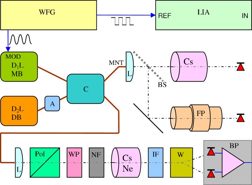
Figure 1: Schematics of the setup. WFG - waveform generator; D₁L - pumping laser (MB) at $894$ nm; D₂L (DB) detection laser at $852$ nm; A - attenuator; C - single mode, polarization maintaining $2\times 2$ fiber coupler; L - lens, BS - beamsplitter, Pol - polarizer; WP - multiorder waveplate acting as quarter-$\lambda$ plate for $894$ nm and as full-$\lambda$ for $852$ nm; NF - neutral filter; Cs-Ne - Cesium cell with buffer gas; IF - interference filter stopping $894$ nm; W - Wollaston analizer; BP- balanced polarimeter for polarization rotation detection, which includes photo diodes and differential transimpedance amplifier; LIA - lockin amplifier. In the monitor (MNT) channel, Cs - Cesium vacuum cell and FP - Fabry-Perot interferometer are used to monitor the radiations’ parameters.

The optical frequency of the MB is monitored by the MNT channel, where the light is sent to a fixed length Fabry-Perot interferometer and to a secondary Cs cell without buffer gas. Both the absorption and the interferometric signals are detected by photo-detection stages with a bandpass largely exceeding the MB modulation frequency. The two diagnostics provide both a relative and an absolute measure of the instantaneous detuning of the MB frequency. The (fixed) DB optical frequency is monitored as well, and it is passively stabilized within 100 MHz.

A sinusoidal signal modulates the optical frequency of the MB at the Larmor frequency, and references a lock-in amplifier detecting the polarization rotation of the DB. The Cs cell is placed in a bias magnetic field of about $600$ nT resulting from the partial compensation of the environmental field. Such bias field results in a Cs magnetic resonance centered at about 2 kHz. The amplitude of the magnetic resonance is registered for various amplitudes of the modulation signal and as a function of the mean MB optical frequency. To this aim the MB optical frequency is slowly scanned by adding a ramp to its modulation signal.

III Model

To develop a theoretical model that describes the time evolution of the monitored magnetization, we consider the whole level structure of the ¹³³Cs $D_{1}$ line. With reference to Fig. 2, the free Hamiltonian in the rotating wave approximation frame reads as

$$H_{0}=\Delta_{g}\,\Pi_{g4}+\delta\,\Pi_{e4}+(\delta-\Delta_{e})\,\Pi_{e3},$$ (1)

where the projector $\Pi_{g4}$ is defined as $\sum_{M}|F_{g}=4,M\rangle\langle F_{g}=4,M|$. Similar expressions hold for the other projectors.

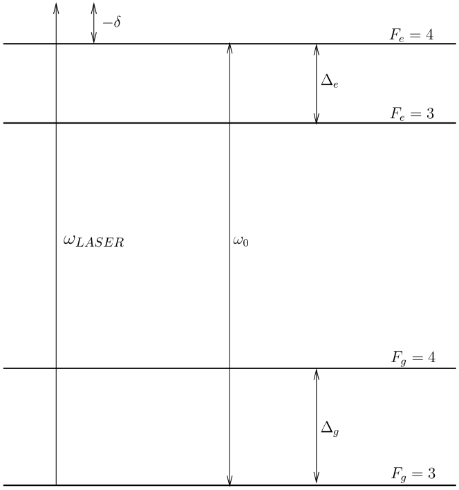
Figure 2: Level scheme of Cs $D_{1}$ line.

To express the interaction with the laser field it is better to adopt a block-matrix notation

$$H_{int}=\begin{pmatrix}0&0&W^{{\dagger}}_{e4,g4}&W^{{\dagger}}_{e4,g3}\\ 0&0&W^{{\dagger}}_{e3,g4}&W^{{\dagger}}_{e3,g3}\\ W_{g4,e4}&W_{g4,e3}&0&0\\ W_{g3,e4}&W_{g3,e3}&0&0\end{pmatrix},$$ (2)

where each matrix element is a sub-matrix defined using the projectors. For instance $W^{{\dagger}}_{e4,g4}=-\Pi_{e4}\,\mathbf{d}\cdot\boldsymbol{\epsilon}\,\Pi_{g4}\;E_{0}$, $W_{g4,e4}=-\Pi_{g4}\,\mathbf{d}\cdot\boldsymbol{\epsilon}^{*}\,\Pi_{e4}\;E_{0}$, etc. Here $\boldsymbol{\epsilon}$ is the laser polarization versor, $E_{0}$ is the amplitude of the laser electric field and $\mathbf{d}$ is the atomic dipole moment.

We need all these blocks in our model, because the laser modulation can be very broad and during the periodic frequency sweep both the ground states may be resonantly excited.

The density operator has a similar block-matrix form

$$\boldsymbol{\rho}=\begin{pmatrix}\rho_{e4}&\rho_{e4,e3}&\rho_{e4,g4}&\rho_{e4,g3}\\ \rho_{e3,e4}&\rho_{e3}&\rho_{e3,g4}&\rho_{e3,g3}\\ \rho_{g4,e4}&\rho_{g4,e3}&\rho_{g4}&\rho_{g4,g3}\\ \rho_{g3,e4}&\rho_{g3,e3}&\rho_{g3,g4}&\rho_{g3}\end{pmatrix}.$$ (3)

The blocks are defined in the manner described above. The diagonal blocks $\rho_{e4},\rho_{e3},\rho_{g4}$, and $\rho_{g3}$ contain both the level populations and the Zeeman coherences. The blocks $\rho_{e4,e3}=\rho_{e3,e4}^{{\dagger}}$ and $\rho_{g4,g3}=\rho_{g3,g4}^{{\dagger}}$ represent the hyperfine coherences, while the remaining blocks represent the optical coherences.

We assume that the hyperfine coherences can be neglected (secular approximation) and with standard methods we write the Bloch equation:

$$\boldsymbol{\dot{\rho}}=-i[H_{0}+H_{int},\boldsymbol{\rho}]+\mathcal{L}_{D}\,\boldsymbol{\rho},$$ (4)

where the Liouvillian $\mathcal{L}_{D}$ takes into account the effects of relaxation processes like spontaneous emission and/or collisions.

As the magnetization is monitored by the DB tuned in the vicinity of the $F_{g}=4\rightarrow J_{e}=3/2$ transition, the signal is substantially given by the $|F_{g}=4\rangle$ state. We assume that the effect of the DB is very weak and its contribution to the Hamiltonian can be neglected. Hence the Bloch equation (4) contains only the MB interaction. To some extent, this approximation is relaxed in the following (see Appendix A).

After some algebra and introducing the irreducible components Omont (1977); Happer (1972)

$$\rho_{g4} =\sum_{k=0}^{2\,F_{g4}}\,\sum_{q=-k}^{k}\;m_{k,q}\;T_{k,q}(g4)$$ (5)

in the hypothesis of weak laser power regime, we find the final equation for the ground state $F_{g}=4$ orientation:

$$\begin{split}\dot{\mathbf{x}}=&i\frac{\omega_{L}}{\sqrt{2}}\begin{pmatrix}-\sqrt{2}(\cos\theta+\gamma)&\sin\theta\operatorname{{\displaystyle e}}^{i\phi}&0\\ \sin\theta\operatorname{{\displaystyle e}}^{-i\phi}&-\sqrt{2}\gamma&\sin\theta\operatorname{{\displaystyle e}}^{i\phi}\\ 0&\sin\theta\operatorname{{\displaystyle e}}^{-i\phi}&\sqrt{2}(\cos\theta-\gamma)\end{pmatrix}\;\mathbf{x}\\ &+P(t)\begin{pmatrix}0\\ 1\\ 0\end{pmatrix}\\ =&A\,\mathbf{x}+P(t)\mathbf{w},\end{split}$$ (6)

where the vector $\mathbf{x}$ is defined as $\mathbf{x}=(m_{1,-1},m_{1,0},m_{1,1})$.

The model produces equations for both the magnetization (orientation) and the alignment, however in this work we discuss only the dynamics of the orientation.

The pumping rate $P(t)$ is reported in the Appendix with full derivation details. Notice that Eq. (6) is essentially equivalent to the Larmor equation with an additional forcing term, being $M_{x}\propto(m_{1,1}-m_{1,-1})$, $M_{y}\propto i(m_{1,1}+m_{1,-1})$ and $M_{z}\propto m_{1,0}$.

The Larmor frequency is $\omega_{L}=g_{Fg}\mu_{B}B$. In our experiment $\omega_{L}$ is in the kHz range, while the relaxation rates (longitudinal and transverse) are in Hz range, so in Eq. (6) we used a single rate $\gamma$. The geometry considered in the model is sketched Fig. 3.

Figure 3: Schematic of the geometry used in the model.

The matrix of coefficients in Eq. (6) can be diagonalized by a Wigner rotation Sakurai and Napolitano (2010) matrix $U$ so that

$$U^{{\dagger}}\,A\,U=A_{D}=\begin{pmatrix}-i\omega_{L}-\gamma&0&0\\ 0&-\gamma&0\\ 0&0&i\omega_{L}-\gamma\end{pmatrix}$$ (7)

and the full solution is

$$\mathbf{x}(t)=U\operatorname{{\displaystyle e}}^{A_{D}\,t}U^{{\dagger}}\,\mathbf{x}(0)+U\int_{0}^{t}\operatorname{{\displaystyle e}}^{A_{D}(t-t^{\prime})}P(t^{\prime})\operatorname{{\displaystyle d}}t^{\prime}\;U^{{\dagger}}\mathbf{w}.$$ (8)

After a time interval much longer than $1/\gamma$, the free solution fades away and the last term sets as the steady-state orientation $\mathbf{x}_{SS}$. Introducing the Fourier components of the pumping term

$$P(t)=\sum_{n=-\infty}^{+\infty}P_{n}\operatorname{{\displaystyle e}}^{i\,n\,\Omega\,t},$$ (9)

where $\Omega\approx\omega_{L}$ is the modulation frequency, one has

$$\mathbf{x}_{SS}=\sum_{n=-\infty}^{+\infty}P_{n}\,\left(U\;\frac{1}{i\,n\,\Omega-A_{D}}\;U^{{\dagger}}\right)\;\mathbf{w}\;\operatorname{{\displaystyle e}}^{i\,n\,\Omega t}.$$ (10)

We are interested in the $z$ component of the magnetization, so that after some straightforward algebra we find

$$\begin{split}M_{z}^{SS}(t)\propto&\;\;\Re(P_{0}C_{0})\\ &+\sum_{n=1}^{+\infty}\bigg{[}\Re(P_{n}C_{n}+P_{-n}C_{-n})\,\cos n\Omega t\\ &\phantom{++\sum_{n=1}^{+\infty}}-\Im(P_{n}C_{n}-P_{-n}C_{-n})\,\sin n\Omega t\bigg{]}\\ \equiv&\;\;a_{0}+\sum_{n}\big{[}a_{n}\cos n\Omega t+b_{n}\sin n\Omega t\big{]},\end{split}$$ (11)

where

$$\begin{split}C_{n}=&\frac{\sin^{2}\theta}{2}\left(\frac{1}{i\,n\,\Omega+\gamma+i\omega_{L}}+\frac{1}{i\,n\,\Omega+\gamma-i\omega_{L}}\right)\\ &+\frac{\cos^{2}\theta}{i\,n\,\Omega+\gamma}.\end{split}$$ (12)

In the experiment, the lock-in amplifier detects the amplitude of the first harmonic $(n=1)$ so we have to evaluate the term $\sqrt{a_{1}^{2}+b_{1}^{2}}$. The coefficients $P_{n}$ satisfy $P_{-n}=P_{n}^{*}$ for each $n$. Additionally, for odd values of $n$ we have $P_{-n}=P_{n}^{*}=-P_{n}$ meaning that for $n=1$ we can assume $P_{1}=iR_{1}$ and $P_{-1}=-iR_{1}$ ($R_{1}$ is a real quantity reported in Appendix A).

Using the condition $\Omega\approx\omega_{L}$ and $\theta=\pi/2,\,\phi=0$ (given by the experimental conditions), after some algebra one finds

$$\mathcal{A}_{1}\equiv\sqrt{a_{1}^{2}+b_{1}^{2}}=\frac{1}{\gamma^{2}+(\Omega-\omega_{L})^{2}}\;|R_{1}|.$$ (13)

Eq. (13) has a clear physical meaning: at low laser power the response of the system is factored out. The first factor gives the usual resonant behaviour when the modulation frequency $\Omega$ is swept over the magnetic resonance line. The second term $R_{1}$ contains the details of the laser frequency modulation and level structure of the $D_{1}$ lines.

The optical frequency of the MB is sinusoidally modulated at the magnetic resonance frequency, so that $\Omega\simeq\omega_{L}$ and the laser detuning $\delta$ from the $D_{1}$ $F_{g}=3\longrightarrow F_{e}=4$ transition (see also Fig. 2) is

$$\delta(t)=\delta_{0}+\Delta\sin\omega_{L}t.$$ (14)

It follows that $R_{1}$ is a function of both $\delta_{0}$ and $\Delta$. Moreover it depends also on the width of the $D_{1}$ one-photon transition $G=\Gamma/2+\Gamma_{c}+\Gamma_{D}$, where $1/\Gamma$ is the radiative lifetime of the excited $D_{1}$ multiplet, $\Gamma_{c}$ represents the broadening due to collisions and $\Gamma_{D}$ is the Doppler broadening. Due to the presence of buffer gas, the excited $D_{1}$ states get depolarized with an additional rate $\Gamma_{c}^{\prime}$, which we added as a phenomenological dependence in $R_{1}$ in a normalized form $r=\Gamma_{c}^{\prime}/\Gamma$. Finally, to model the influence of the DB, a parameter $\alpha$, describing a global population imbalance of the two ground hyperfine states is also introduced.

Appendix A contains a full derivation and discussion about the explicit form of $R_{1}$, as well as a detailed definition of the parameter $\alpha$.

IV Results

In this section we report experimental measurements obtained in different regimes, and compare them with the theoretical profiles.

Beside atomic constants, the model contains several parameters ($\delta_{0}$, $\Delta$, $r$, and $G$) fixed by the experimental conditions, and only one quantity, $\alpha$, which is a free parameter. In our conditions $\Gamma\approx 5$ MHz, and the broadening due to collisions is dominant, as $\Gamma_{c}\approx 500$ MHz at 90 Torr of He, and $\Gamma_{D}\approx 200$MHz, thus we use $G=0.5$ GHz in almost all the simulations.

Concerning $r$, it is known since the Sixties Franz and Franz (1966); Baylis (1979) that the collisions with the buffer gas atoms are effective in depolarizing the $D_{2}$ excited states, while perturb weakly the $D_{1}$ ${}^{2}P_{1/2}$ states. Moreover our theoretical results do not depend strongly on the value of $r$, and we have assumed $r=0.5$ in all the the simulations.

The only free parameter – $\alpha$ – is chosen to obtain the best correspondence between the measured and the simulated signals. As shown below, a value of $\alpha\approx 0.25$ leads to a good comparison, a clear indication that, in spite of its very low power, DB has a not negligible influence.

As for the modulation amplitude $\Delta$, it has to be compared to $\Delta_{g}$, and three regimes can be identified: small, i.e. $2\Delta\ll\Delta_{g}$, intermediate ($2\Delta\approx\Delta_{g}$) and large ($2\Delta\gg\Delta_{g}$) modulation amplitude respectively. In the following we discuss these three regimes.

Figure 4 shows the signal obtained for $\Delta=0.5$ GHz. As predicted by Eq.(29), the four $D_{1}$ transitions give eight peaks in $R_{1}$, separated in two groups around the positions of the two hyperfine ground-states, corresponding to $\delta_{0}/\Delta_{g}\approx 0$ and $\delta_{0}/\Delta_{g}\approx 1$. These peaks are well resolved in conditions of small collisional broadening as can be noticed in Fig. 4 (a). Here the experimental signal is recorded with a lower buffer gas pressure giving a nominal $\Gamma_{c}\approx 18$ MHz, so to compare we used the value $G=200$ MHz. Increasing the collisional broadening up to 0.5 GHz, some peaks overlap as can be seen in the Fig. 4 (b).

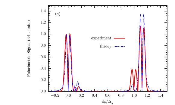
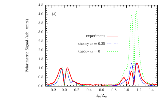
Figure 4: (Color online) Comparison of theoretical and experimental signals as a function of $\delta_{0}/\Delta_{g}$ in a regime of small modulation. For both plots the following values have been used in the model: $2\Delta=0.5$ GHz, $r=0.5$, $\alpha=0.25$, $\Delta_{e}=1.1$ GHz and $\Delta_{g}=9.2$ GHz. The plots show magnetic resonances amplitudes as obtained with (a) low buffer gas pressure (2 Torr Ar) and (b) high buffer gas pressure (90 Torr Ne). Correspondingly $G=200$ MHz and $G=500$ MHz are used in the simulations. In the plot (b) we report for comparison also the model output obtained with $\alpha=0$.

In all the plots, we normalize to 1 the height of the leftmost peaks, both measured and simulated. The value of $\alpha$ is chosen in such a way to reproduce rightmost peaks height matching the experimental observation. With $\alpha=0$ the right peak results four times higher than the first one (see the green-dashed line in Fig. 4 (b)). A good accordance between the measured and simulated resonance amplitudes is found for $\alpha\approx 0.25$.

It is remarkable that when the MB is mainly resonant with the $F_{g}=3$ transitions (e.g. $\delta_{0}\approx-\Delta$) the recorded signal has peak value comparable with the one obtained with ($\delta_{0}\approx\Delta_{g}$), in spite of the fact that the measured quantity is the magnetization in the $F_{g}=4$ ground state. At $\delta_{0}\approx-\Delta$, the MB causes a strong hyperfine pumping towards the $F_{g}=4$ state. Thus, despite the fact that the laser is not in resonance with the $F_{g}=4$ sublevels, a high degree of Zeeman pumping is observed. Thus the leftmost peak appearing in the plot corresponds to an interaction condition where the MB produces a high amplitude magnetic resonance, while weakly perturbing the hyperfine ground state where the magnetization is induced. This interaction regime has been successfully used (in a regime of stronger MB intensity) for high sensitivity magnetometry Bevilacqua et al. (2016a).

As shown in Fig.5, the model reproduces with good accurateness the signal behavior also in the intermediate regime where $2\Delta\approx\Delta_{g}$. In this case, the MB may resonantly excite either one or both the ground states simultaneously, which happens for $\delta_{0}/\Delta_{g}\approx 1/2$. A good agreement between the theoretical and experimental results is obtained keeping the same values of the parameters. In this case the eight components merge into four peaks of comparable height and nearly symmetric shape.

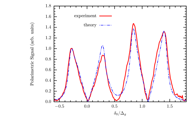
Figure 5: (Color online) Comparison of theoretical and experimental signals as a function of $\delta_{0}$ in the intermediate regime. The following values have been used: $G=0.5$ GHz, $2\Delta=5.6$ GHz, $\Gamma_{c}^{\prime}/\Gamma=0.5$, $\alpha=0.25$, $\Delta_{e}=1.1$ GHz and $\Delta_{g}=9.2$ GHz.

The results corresponding to the third regime, where $2\Delta$ exceeds $\Delta_{g}$, are shown in Fig. 6. Here, some technical limitations prevent the possibility to extend the scan at higher values of $\delta_{0}$, so that a rightmost peak corresponding to $L_{eg}$ (see Eq. (17d)) is not recorded. The leftmost peak has a maximum at $\delta_{0}\approx-\Delta$, according to what is expected from Eq.(17). The peaks observed experimentally have an asymmetric shape more evident at large values of $\Delta$, this feature is well reproduced by the model. On the other hand, similarly to what appears in Fig. 4 some discrepancies emerges more visibly at $\delta_{0}\approx\Delta_{g}$. There is experimental evidence that the DB, in spite of its very weak intensity, is responsible for these minor deviations: those discrepancies actually change with the intensity and the detuning of DB.

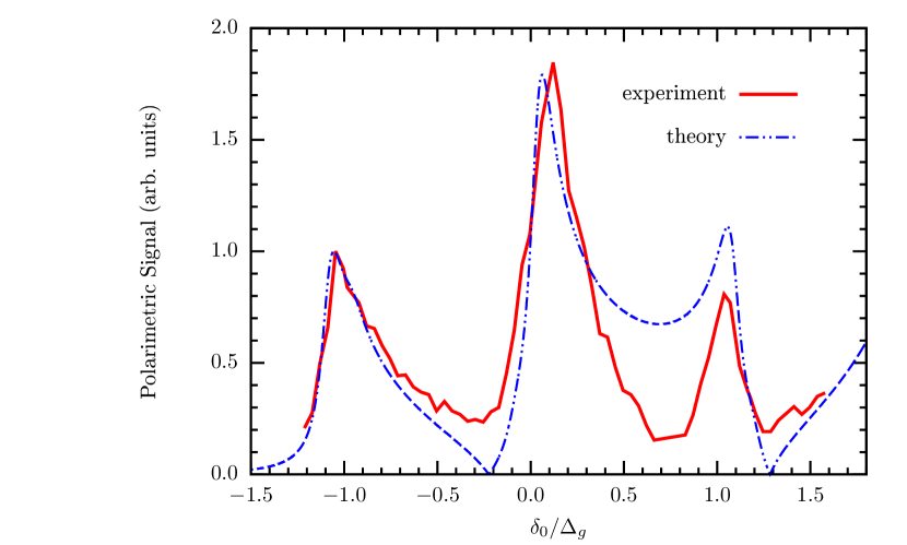
Figure 6: (Color online) Comparison between theoretical and experimental signals as a function of $\delta_{0}$ in the regime with $2\Delta\gg\Delta_{g}$. The following values have been used: $G=0.5$ GHz, $2\Delta=20.0$ GHz, $\Gamma_{c}^{\prime}/\Gamma=0.5$, $\alpha=0.20$, $\Delta_{e}=1.1$ GHz and $\Delta_{g}=9.2$ GHz.

V Conclusion

A model is developed to describe the behavior of magnetic resonances measured in Cesium vapour in an experiment where a weak intensity laser radiation tuned to the D₁ transitions is broadly frequency modulated. Such modulation makes the laser-atom interaction occur in a condition where both the hyperfine ground levels are excited. In the approximation of weak intensity, a multipole expansion analysis enables an accurate evaluation of the measured quantity that is the time dependent magnetization of atoms in the $F_{g}=4$ state. A comparison with the experiment is made in three regimes, where the modulation depth is smaller, comparable or larger than the ground state hyperfine splitting, respectively. A good correspondence is found, and the model reproduces satisfactorily the recorded features with the requirement of tuning only one free parameter ($\alpha$). This parameter is phenomenologically introduced to account for an imbalance in the populations of the $F_{g}=3$ and $F_{g}=4$ states that is induced by the detection radiation.

Appendix A Derivation of the pumping term

Rewriting the Eq. (4) for each block of $\boldsymbol{\rho}$ and assuming the adiabatic approximation Stenholm (2005) for the optical coherences, for instance we find

$$\rho_{e_{4},g_{4}}=\frac{i}{G+i(\delta-\Delta_{g})}\;\big{[}\rho_{e4,e4}\;W^{{\dagger}}_{e4,g4}-W^{{\dagger}}_{e4,g4}\;\rho_{g4,g4}\big{]}$$ (15)

and similar expressions for the other optical coherences which we do not report explicitly. In (15) $G$ is the width of the $D_{1}$ one-photon transition determined as $G=\Gamma/2+\Gamma_{c}$ ($1/\Gamma$ is the lifetime of the excited $D_{1}$ multiplet and $\Gamma_{c}$ represents additional broadening due to collisions). Finally $\delta$ is the laser detuning from the $F_{g}=3\rightarrow F_{e}=4$ transition (see also Fig. 2).

Substituting the expressions like (15) in the equations for the diagonal blocks of $\boldsymbol{\rho}$ we find

$$\begin{split}\dot{\rho}_{e4}=&-\Gamma\rho_{e4}+{\cal L}_{coll}(\rho_{e4})\\ &-i[D_{0}W^{{\dagger}}_{e4,g3}W_{g3,e4}+D_{g}W^{{\dagger}}_{e4,g4}W_{g4,e4},\rho_{e4}]\\ &-\{L_{0}W^{{\dagger}}_{e4,g3}W_{g3,e4}+L_{g}W^{{\dagger}}_{e4,g4}W_{g4,e4},\rho_{e4}\}\\ &+2L_{0}W^{{\dagger}}_{e4,g3}\;\rho_{g3}\;W_{g3,e4}\\ &+2L_{g}W^{{\dagger}}_{e4,g4}\;\rho_{g4}\;W_{g4,e4},\end{split}$$ (16a)

where $${\cal L}_{coll} {\cal L}_{coll} k\geq 1$$ takes into account the collision effects in the excited state. We assume that is diagonal and quenches the multipoles with (see below).

Similarly one obtains

$$\begin{split}\dot{\rho}_{g4}=&-\gamma\rho_{g4}-i[-\boldsymbol{\mu}\cdot\mathbf{B},\rho_{g4}]\\ &-i[D_{g}W_{g4,e4}W^{{\dagger}}_{e4,g4}+D_{eg}W_{g4,e3}W^{{\dagger}}_{e3,g4},\rho_{g4}]\\ &-\{L_{g}W_{g4,e4}W^{{\dagger}}_{e4,g4}+L_{eg}W_{g4,e3}W^{{\dagger}}_{e3,g4},\rho_{g4}\}\\ &+2L_{g}W_{g4,e4}\;\rho_{e4}\;W^{{\dagger}}_{e4,g4}\\ &+2L_{eg}W_{g4,e3}\;\rho_{e3}\;W^{{\dagger}}_{e3,g4}\\ &+\mathcal{R}_{s.e}.\end{split}$$ (16b)

Analogous expressions are obtained for the other diagonal blocks of $\boldsymbol{\rho}$. From Eq. (16) we can infer that the laser gives a Hamiltonian contribution (term with the commutator) as well as a relaxation (term with the anti-commutator) to the dynamics of the excited and ground states multiplets. In (16) we have introduced the abbreviations

$$\frac{1}{G+i\delta} =L_{0}-iD_{0},$$ (17a)

$$\frac{1}{G+i(\delta-\Delta_{e})} =L_{e}-iD_{e},$$ (17b)

$$\frac{1}{G+i(\delta-\Delta_{g})} =L_{g}-iD_{g},$$ (17c)

$$\frac{1}{G+i(\delta-\Delta_{g}-\Delta_{e})} =L_{eg}-iD_{eg},$$ (17d)

and $\mathcal{R}_{s.e.}$ represents the spontaneous emission contributions, whose explicit expressions in term of irreducible components (see below) are reported by Dumont Dumont and Decomps (1968). In addition, we neglect the excited state dynamics due to the magnetic field and added a phenomenological relaxation constant $\gamma$ in the ground state.

To proceed further we assume the low laser power limit and completely un-polarized ground states

$$W\rightarrow \;\eta W$$ (18a)

$$W^{{\dagger}}\rightarrow \;\eta W^{{\dagger}}$$ (18b)

$$\rho_{e4}= \;\eta^{2}\rho_{e4}^{(2)}+O(\eta^{4})$$ (18c)

$$\rho_{e3}= \;\eta^{2}\rho_{e3}^{(2)}+O(\eta^{4})$$ (18d)

$$\rho_{g4}= \;\left(\frac{1}{2}-\alpha\right)\frac{\Pi_{g4}}{2F_{g4}+1}+\eta^{2}\rho_{g4}^{(2)}+O(\eta^{4})$$ (18e)

$$\rho_{g3}= \;\left(\frac{1}{2}+\alpha\right)\frac{\Pi_{g3}}{2F_{g3}+1}+\eta^{2}\rho_{g3}^{(2)}+O(\eta^{4}),$$ (18f)

where $\eta$ is a very small parameter quantifying the approximation. Here the factors $1/2\pm\alpha$ ($-1/2\leq\alpha\leq 1/2$) account, in a phenomenological way, for the pumping effects of the DB. When $\alpha=0$ the DB is an ideal probe laser not disturbing the ground state dynamics. A positive value of $\alpha$ denotes an increase of the $F_{g}=3$ global population and a decrease of the $F_{g}=4$ one. A negative value of $\alpha$ would describe the other way around. Introducing the populations imbalance in such simplified way corresponds to neglect the Zeeman sublevels structure of the ground states and the details of their interaction with the DB: in other word $\alpha\neq 0$ reproduces only a global population imbalance between the two hyperfine ground states, while excluding any polarization effect.

To proceed it is better to introduce the irreducible components Omont (1977); Happer (1972) of each density matrix block

$$\rho_{g4}^{(2)}=\sum_{k=0}^{2F_{g4}}\sum_{q=-k}^{k}(\rho_{g4}^{(2)})_{k,q}\;T_{k,q}(g4),$$ (19)

where the irreducible tensor operators

$$\begin{split}T_{k,q}(g4)=&\sqrt{2k+1}\sum_{M}(-1)^{F_{g4}-M}\begin{pmatrix}F_{g4}&F_{g4}&k\\ M&q-M&-q\end{pmatrix}\\ &\times|F_{g4}M\rangle\langle F_{g4}M-q|\end{split}$$ (20)

are expressed using the Wigner 3j coefficients. Similar expressions can be written for the remaining blocks.

The effect of collisional damping in the excited state is modeled as

$$({\cal L}_{coll}(\rho_{e4}^{(2)}))_{k,q}=-\Gamma_{c}^{\prime}\;(\rho_{e4}^{(2)})_{k,q}\qquad k\geq 1.$$ (21)

The ground state feeding by spontaneous emission described by $\mathcal{R}_{s.e.}$ in Eq. (16b) assumes a simple form for the irreducible components Dumont and Decomps (1968)

$$\big{[}\mathcal{R}_{s.e.}(e\rightarrow g)\big{]}_{k,q}=\xi_{k}(J_{e},Fe,J_{g},Fg)\;(\rho_{e})_{k,q},$$ (22)

where

$$\begin{split}\xi_{k}(J_{e},F_{e},J_{g},F_{g})=&(2J_{e}+1)(2F_{g}+1)(2F_{e}+1)\\ &(-1)^{F_{e}+F_{g}+k+1}\Gamma\\ &\left\{\begin{matrix}F_{e}&F_{g}&1\\ J_{g}&J_{e}&I\end{matrix}\right\}^{2}\left\{\begin{matrix}F_{g}&F_{g}&k\\ F_{e}&F_{e}&1\end{matrix}\right\}.\end{split}$$ (23)

After some algebra Eq. (16b) becomes

$$\begin{split}\frac{\operatorname{{\displaystyle d}}}{\operatorname{{\displaystyle d}}t}(\rho_{g4}^{(2)})_{k,q}\bigg{|}_{LASER}=&\;\left(\frac{1}{2}-\alpha\right)\frac{L_{g}}{9}\bigg{[}-(W_{g4,e4}W_{e4,g4}^{{\dagger}})_{k,q}+\frac{\xi_{k}(e4\rightarrow g4)}{\Gamma_{c}^{\prime}}(W_{e4,g4}^{{\dagger}}W_{g4,e4})_{k,q}\bigg{]}+\\ &\;\left(\frac{1}{2}-\alpha\right)\frac{L_{eg}}{9}\bigg{[}-(W_{g4,e3}W_{e3,g4}^{{\dagger}})_{k,q}+\frac{\xi_{k}(e3\rightarrow g4)}{\Gamma_{c}^{\prime}}(W_{e3,g4}^{{\dagger}}W_{g4,e3})_{k,q}\bigg{]}+\\ &\;\left(\frac{1}{2}+\alpha\right)\frac{1}{7}\bigg{[}L_{0}\frac{\xi_{k}(e4\rightarrow g4)}{\Gamma_{c}^{\prime}}(W_{e4,g3}^{{\dagger}}W_{g3,e4})_{k,q}+L_{e}\frac{\xi_{k}(e3\rightarrow g4)}{\Gamma_{c}^{\prime}}(W_{e3,g3}^{{\dagger}}W_{g3,e3})_{k,q}\bigg{]}.\end{split}$$ (24)

Using standard methods (see Omont (1977)) the irreducible components of $W\,W^{{\dagger}}$ and $W^{{\dagger}}W$ can be worked out

$$(W_{g_{i},e_{j}}W_{e_{j},g_{i}}^{{\dagger}})_{k,q} =E_{0}^{2}\langle F_{e_{j}}||\mathbf{d}||F_{g_{i}}\rangle^{2}(-1)^{F_{e_{j}}-F_{g_{i}}}\left\{\begin{matrix}1&1&k\\ F_{g_{i}}&F_{g_{i}}&F_{e_{j}}\end{matrix}\right\}\,(-1)^{q}\mathbb{E}_{k,-q}$$ (25a)

$$(W_{e_{j},g_{i}}^{{\dagger}}W_{g_{i},e_{j}})_{k,q} =E_{0}^{2}\langle F_{e_{j}}||\mathbf{d}||F_{g_{i}}\rangle^{2}(-1)^{F_{g_{i}}-F_{e_{j}}}\left\{\begin{matrix}1&1&k\\ F_{e_{j}}&F_{e_{j}}&F_{g_{i}}\end{matrix}\right\}\,(-1)^{q}\mathbb{E}_{k,-q}.$$ (25b)

The reduced matrix element of the dipole can be rewritten as Judd (2014)

$$\begin{split}\langle F_{e_{j}}||\mathbf{d}||F_{g_{i}}\rangle&\equiv\langle(J_{e}I)F_{e_{j}}||\mathbf{d}||(J_{g}I)F_{g_{i}}\rangle\\ &=(-1)^{J_{e}+I+F_{g_{i}}+1}\sqrt{(2F_{e_{j}}+1)(2F_{g_{i}}+1)}\left\{\begin{matrix}F_{e_{j}}&1&F_{g_{i}}\\ J_{g}&I&J_{e}\end{matrix}\right\}\langle J_{e}||\mathbf{d}||J_{g}\rangle,\end{split}$$ (26)

while the polarization tensor $\mathbb{E}_{k,q}$ is constructed from the laser polarization vector as

$$\mathbb{E}_{K,Q}=(-1)^{K+Q}\sqrt{2K+1}\sum_{q,q^{\prime}=-1}^{1}\begin{pmatrix}1&1&K\\ q&q^{\prime}&Q\end{pmatrix}\;(\epsilon^{*})_{-q}\,\epsilon_{-q^{\prime}},$$ (27)

which for circular $\sigma^{+}$ polarization becomes

$$\mathbb{E}_{k,q}=-\delta_{q,0}\left(\frac{1}{\sqrt{3}}\delta_{k,0}+\frac{1}{\sqrt{2}}\delta_{k,1}+\frac{1}{\sqrt{6}}\delta_{k,2}\right).$$ (28)

Putting all together Eq. (24) becomes

$$\begin{split}\frac{\operatorname{{\displaystyle d}}}{\operatorname{{\displaystyle d}}t}(\rho_{g4}^{(2)})_{1,q}\bigg{|}_{LASER}=&-\frac{\sqrt{15}}{20736}E_{0}^{2}\langle J_{e}||\mathbf{d}||J_{g}\rangle^{2}\frac{1}{1+r}\times\\ &\bigg{[}(1-2\alpha)(29+48r)\,L_{g}\\ &\phantom{+}+21(1-2\alpha)(25+16r)L_{eg}\\ &\phantom{+}-171(1+2\alpha)L_{0}-27(1+2\alpha)L_{e}\bigg{]}\delta_{q,0},\end{split}$$ (29)

where $r=\Gamma_{c}^{\prime}/\Gamma$. Dropping the constant (irrelevant at this order of approximation) in front of the expression, this is exactly the $P(t)$ function used in Eq. (9). The time-dependence arises from the laser modulation, i.e., in Eq. (17) the substitution $\delta\rightarrow\delta_{0}+\Delta\sin\Omega t$.

The Fourier coefficients $P_{n}$ of Eq. (9) have an analytical form. In fact re-doing the steps of Arndt (1965) one finds ($n\geq 0$)

$$\begin{split}P_{n}^{(0)}\equiv&\frac{\Omega}{2\pi}\int_{0}^{2\pi/\Omega}\operatorname{{\displaystyle e}}^{-i\,n\,\Omega\,t}\,L_{0}(t)\operatorname{{\displaystyle d}}t\\ =&\frac{1}{2\pi}\int_{0}^{2\pi}\operatorname{{\displaystyle e}}^{-i\,n\,\theta}\,\frac{G}{G^{2}+(\delta_{0}+\Delta\sin\theta)^{2}}\operatorname{{\displaystyle d}}\theta\\ =&\frac{1}{2}\int_{-\infty}^{+\infty}J_{n}(z\Delta)\operatorname{{\displaystyle e}}^{i\,z\,\delta_{0}}\operatorname{{\displaystyle e}}^{-G\,|z|}\operatorname{{\displaystyle d}}z\\ =&\begin{cases}\Re(I_{n})&n\;\mathrm{even}\\ i\Im(I_{n})&n\;\mathrm{odd},\end{cases}\end{split}$$ (30)

where

$$\begin{split}I_{n}\equiv&\int_{0}^{+\infty}J_{n}(z\Delta)\operatorname{{\displaystyle e}}^{i\,z\,\delta_{0}}\operatorname{{\displaystyle e}}^{-G\,z}\operatorname{{\displaystyle d}}z\\ =&\frac{1}{\Delta^{n}}\frac{\bigg{[}\sqrt{(G-i\delta_{0})^{2}+\Delta^{2}}-(G-i\delta_{0})\bigg{]}^{n}}{\sqrt{(G-i\delta_{0})^{2}+\Delta^{2}}}\end{split}$$ (31)

and the last step follows from formula (6.611) of Gradshteyn and Ryzhik (2007). So the first harmonic coefficient reads as (see also Eq. (13))

$$R_{1}^{(0)}=-\frac{1}{\Delta}\Im\left(\frac{G-i\delta_{0}}{\Delta}\,\frac{1}{\sqrt{1+\left(\frac{G-i\delta_{0}}{\Delta}\right)^{2}}}\right),$$ (32)

which can be rewritten using the dispersive and absorptive profiles

$$\mathcal{D}(\delta_{0}) =\frac{\delta_{0}-\Delta}{(\delta_{0}-\Delta)^{2}+G^{2}}-\frac{\delta_{0}+\Delta}{(\delta_{0}+\Delta)^{2}+G^{2}}$$ (33a)

$$\mathcal{L}(\delta_{0}) =\frac{1}{(\delta_{0}-\Delta)^{2}+G^{2}}+\frac{1}{(\delta_{0}+\Delta)^{2}+G^{2}}$$ (33b)

as

$$R_{1}^{(0)}=-\frac{1}{\sqrt{2}\Delta}\,\mathrm{sign}(-\delta_{0})\left[\sqrt{1+\Delta\frac{G^{2}+3\Delta^{2}/4}{G^{2}+\Delta^{2}}\left(\mathcal{D}(\delta_{0})+\frac{\Delta^{2}}{4G^{2}+3\Delta^{2}}\mathcal{L}(\delta_{0})\right)}-1-(\Delta/2)\mathcal{D}(\delta_{0})\right]^{1/2}.$$ (34)

This is the contribution of $L_{0}(t)$ that is the $F_{g}=3\rightarrow F_{e}=4$ line and it is shown in Fig. 7.

Similar expressions hold for the other transitions and adding all together with the coefficients of Eq. (29) we obtain the whole $R_{1}$ which contains the dependence from the laser modulation parameters.

Figure 7: (Color online) Typical profile obtained from the excitation of a single transition. The peaks are located in correspondence of $\delta_{0}\approx\pm\Delta$ for $G/\Delta\lesssim 1$. At larger values of $G$ the peaks broaden and start shifting in opposite directions.

References

- William Happer et al. (2010) William Happer, Yuan-Yu Jau, and Thad Walker, Optically pumped atoms (Wiley-VCH verlag GmbH KGaA Leipzig, 2010), ISBN 978-3-527-62951-0.
- Happer (1972) W. Happer, Rev. Mod. Phys. 44, 169 (1972), URL http://link.aps.org/doi/10.1103/RevModPhys.44.169.
- Metcalf and van der Straten (1999) H. J. Metcalf and P. van der Straten, Laser Cooling and Trapping (Springer Verlag, New York, 1999), ISBN 978-0-387-98728-6.
- abd Ruvin Ferber (2005) M. A. abd Ruvin Ferber, Optical Polarization of Molecules (Cambridge University Press, Cambridge UK, 2005), ISBN 978-0-521-67344-0.
- Aleksandrov and Vershovskii (2009) E. B. Aleksandrov and A. K. Vershovskii, Physics-Uspekhi 52, 573 (2009), URL http://stacks.iop.org/1063-7869/52/i=6/a=R06.
- Lenci et al. (2014) L. Lenci, A. Auyuanet, S. Barreiro, P. Valente, A. Lezama, and H. Failache, Phys. Rev. A 89, 043836 (2014), URL http://link.aps.org/doi/10.1103/PhysRevA.89.043836.
- Budker and Romalis (2007) D. Budker and M. Romalis, Nature Physics 3, 227 (2007), eprint physics/0611246.
- Suter and Mlynek (1991) D. Suter and J. Mlynek, Phys. Rev. A 43, 6124 (1991), URL http://link.aps.org/doi/10.1103/PhysRevA.43.6124.
- Schultze et al. (2012) V. Schultze, R. Ijsselsteijn, T. Scholtes, S. Woetzel, and H.-G. Meyer, Opt. Express 20, 14201 (2012), URL http://www.opticsexpress.org/abstract.cfm?URI=oe-20-13-14201.
- Rosatzin et al. (1990) M. Rosatzin, D. Suter, W. Lange, and J. Mlynek, J. Opt. Soc. Am. B 7, 1231 (1990), URL http://josab.osa.org/abstract.cfm?URI=josab-7-7-1231.
- Klepel and Suter (1992) H. Klepel and D. Suter, Optics Communications 90, 46 (1992), ISSN 0030-4018, URL http://www.sciencedirect.com/science/article/pii/003040189290%325L.
- Breschi et al. (2013) E. Breschi, Z. D. Gruijc, P. Knowles, and A. Weis, Phys. Rev. A 88, 022506 (2013), URL http://link.aps.org/doi/10.1103/PhysRevA.88.022506.
- Breschi et al. (2014) E. Breschi, Z. D. Grujic, P. Knowles, and A. Weis, Applied Physics Letters 104, 023501 (2014), URL http://scitation.aip.org/content/aip/journal/apl/104/2/10.106%3/1.4861458.
- Bevilacqua and Breschi (2014) G. Bevilacqua and E. Breschi, Phys. Rev. A 89, 062507 (2014), URL http://link.aps.org/doi/10.1103/PhysRevA.89.062507.
- Belfi et al. (2007) J. Belfi, G. Bevilacqua, V. Biancalana, Y. Dancheva, and L. Moi, Journal of the Optical Society of America B Optical Physics 24, 1482 (2007), eprint 0705.1671.
- Acosta et al. (2006) V. Acosta, M. P. Ledbetter, S. M. Rochester, D. Budker, D. F. Jackson Kimball, D. C. Hovde, W. Gawlik, S. Pustelny, J. Zachorowski, and V. V. Yashchuk, Phys. Rev. A 73, 053404 (2006), URL http://link.aps.org/doi/10.1103/PhysRevA.73.053404.
- Zigdon et al. (2010) T. Zigdon, A. D. Wilson-Gordon, S. Guttikonda, E. J. Bahr, O. Neitzke, S. M. Rochester, and D. Budker, Opt. Express 18, 25494 (2010), URL http://www.opticsexpress.org/abstract.cfm?URI=oe-18-25-25494.
- Bevilacqua et al. (2012) G. Bevilacqua, V. Biancalana, Y. Dancheva, and L. Moi, Phys. Rev. A 85, 042510 (2012), eprint 1112.1309.
- Sheng et al. (2013) D. Sheng, S. Li, N. Dural, and M. Romalis, Phys. Rev. Lett. 110, 160802 (2013), URL http://link.aps.org/doi/10.1103/PhysRevLett.110.160802.
- Wolf et al. (2015) T. Wolf, P. Neumann, K. Nakamura, H. Sumiya, T. Ohshima, J. Isoya, and J. Wrachtrup, Phys. Rev. X 5, 041001 (2015), URL http://link.aps.org/doi/10.1103/PhysRevX.5.041001.
- Sydoryk et al. (2008) I. Sydoryk, N. N. Bezuglov, I. I. Beterov, K. Miculis, E. Saks, A. Janovs, P. Spels, and A. Ekers, Phys. Rev. A 77, 042511 (2008), URL http://link.aps.org/doi/10.1103/PhysRevA.77.042511.
- Bevilacqua et al. (2016a) G. Bevilacqua, V. Biancalana, P. Chessa, and Y. Dancheva, appearing in Applied Physics B (2016a), URL http://arxiv.org/pdf/1601.06938.pdf.
- Bevilacqua et al. (2013) G. Bevilacqua, V. Biancalana, Y. Dancheva, and L. Moi, in Annual Reports on NMR Spectroscopy, edited by G. A. Webb (Academic Press, 2013), vol. 78, pp. 103 – 148, URL http://www.sciencedirect.com/science/article/pii/B97801240471%67000031.
- Bevilacqua et al. (2009) G. Bevilacqua, V. Biancalana, Y. Dancheva, and L. Moi, Journal of Magnetic Resonance 201, 222 (2009), eprint 0906.1089.
- Bevilacqua et al. (2016b) G. Bevilacqua, V. Biancalana, A. B.-A. Baranga, Y. Dancheva, and C. Rossi, Journal of Magnetic Resonance 263, 65 (2016b), ISSN 1090-7807, URL http://www.sciencedirect.com/science/article/pii/S10907807150%03195.
- Omont (1977) A. Omont, Irreducible Components of the Density Matrix: Application to Optical Pumping, Progress in quantum electronics (Pergamon Press, 1977), ISBN 9780080216478, URL http://books.google.it/books?id=R28EywAACAAJ.
- Sakurai and Napolitano (2010) J. J. Sakurai and J. J. Napolitano, Modern Quantum Mechanics (Addison Wesley, 2010), 2nd ed.
- Franz and Franz (1966) F. A. Franz and J. R. Franz, Phys. Rev. 148, 82 (1966), URL http://link.aps.org/doi/10.1103/PhysRev.148.82.
- Baylis (1979) W. E. Baylis, Progress in Atomic Spectroscopy: Part B (Springer US, Boston, MA, 1979), chap. Collisional Depolarization in the Excited State, pp. 1227–1297, ISBN 978-1-4613-3935-9, URL http://dx.doi.org/10.1007/978-1-4613-3935-9_13.
- Stenholm (2005) S. Stenholm, Foundations of laser spectroscopy, Dover Books on Physics (Dover Publications, 2005), ISBN 0486444988.
- Dumont and Decomps (1968) M. Dumont and B. Decomps, J. Phys. France 29, 181 (1968).
- Judd (2014) B. R. Judd, Operator Techniques in Atomic Spectroscopy (Princeton University Press, 2014), ISBN 9780691604275.
- Arndt (1965) R. Arndt, Journal of Applied Physics 36, 2522 (1965), URL http://scitation.aip.org/content/aip/journal/jap/36/8/10.1063%/1.1714523.
- Gradshteyn and Ryzhik (2007) I. S. Gradshteyn and I. M. Ryzhik, Table of integrals, series, and products (Elsevier/Academic Press, Amsterdam, 2007), seventh ed., ISBN 978-0-12-373637-6, translated from the Russian, Translation edited and with a preface by Alan Jeffrey and Daniel Zwillinger, With one CD-ROM (Windows, Macintosh and UNIX).