Optimal Energy-Efficient Downlink Transmission Scheduling for Real-Time Wireless Networks

Abstract

It has been shown that using appropriate channel coding schemes in wireless environments, transmission energy can be significantly reduced by controlling the packet transmission rate. This paper seeks optimal solutions for downlink transmission control problems, motivated by this observation and by the need to minimize energy consumption in real-time wireless networks. Our problem formulation deals with a more general setting than the paper authored by Gamal et. al., in which the MoveRight algorithm is proposed. The MoveRight algorithm is an iterative algorithm that converges to the optimal solution. We show that even under the more general setting, the optimal solution can be efficiently obtained through an approach decomposing the optimal sample path through certain “critical tasks” which in turn can be efficiently identified. We include simulation results showing that our algorithm is significantly faster than the MoveRight algorithm. We also discuss how to utilize our results and receding horizon control to perform on-line transmission scheduling where future task information is unknown.

I Introduction

Because wireless nodes are normally powered by batteries and are expected to remain in operation for extended periods of time, how to conserve energy in order to extend node lifetime and network lifetime is a major research issue in most wireless networks. One way of saving energy is to operate these nodes at low power as long as possible. However, this will also significantly downgrade their functionality. Therefore, there is a trade-off between energy and the “quality” delivered by wireless nodes. When “quality” is measured in terms of latency, the trade-off is between energy and time. Examples arise in real-time computing, where a processor trades off processing rate for energy [1]; and in wireless transmission, where a transmitter trades off transmission speed for energy [2].

When the energy of a wireless node is consumed mostly by communication tasks, scheduling a RF transmission efficiently becomes extremely important in conserving the energy of the node. It is well known that there exists an explicit relationship between transmission power and channel capacity [3]; transmission power can be adjusted by changing the transmission rate, provided that appropriate coding schemes are used. This provides an option to conserve the transmission energy of a wireless node by slowing down the transmission rate. Increased latency is a direct side effect caused by the low transmission rate and it can affect other Quality-of-Service (QoS) metrics as well. For example, excessive delay may cause buffer overflow, which increases the packet dropping rate. The existence of this trade-off between energy and latency motivates Dynamic Transmission Control techniques for designing energy-efficient wireless systems.

To the best of our knowledge, the earliest work that captures the trade-off between energy and latency in transmission scheduling is [4], in which Collins and Cruz formulated a Markov decision problem for minimizing transmission cost subject to some power constraints. By assuming a linear dependency between transmission cost and time, their model did not consider the potential of more energy saving by varying the transmission rate. Berry [5] considered a Markov decision process in the context of wireless fading channels to minimize the weighted sum of average transmission power and a buffer cost, which corresponds to either average delay or probability of buffer overflow. Using dynamic programming and assuming the transmission cost to be a convex function of time, Berry discovered some structural properties of the optimal adaptive control policy, which relies on information on the arrival state, the queue state, and the channel state. In [6] and [7], Ata developed optimal dynamic power control policies subject to a QoS constraint for Markovian queues in wireless static channels and fading channels respectively. In his work, the optimization problem was formulated to minimize the long-term average transmission power, given a constraint of buffer overflow probability in equilibrium; dynamic programming and Lagrangian relaxation approaches were used in deriving the optimal policies, which can be expressed as functions of the packet queue length and the channel state. Neely utilized a Lyapunov drift technique in [8] to develop a dynamic power allocation and routing algorithm that minimizes the average power of a cell-partitioned wireless network. It was shown that the on-line algorithm operates without knowledge of traffic rates or channel statistics, and yields average power that is arbitrarily close to the off-line optimal solution. A related problem of maximizing throughput subject to peak and average power constraints was also discussed in [8].

Today’s real-time data communications require Quality-of-Service (QoS) guarantee for each individual packet. Another line of research aims at minimizing the transmission energy over a single wireless link while providing QoS guarantee. In particular, it is assumed that each packet is associated with an arrival time (generally random), a number of bits, a hard deadline that must be met, and an energy function. This line of work was initially studied in [9] with follow-up work in [2] where a ”homogeneous” case is considered assuming all packets have the same deadline and number of bits. By identifying some properties of this convex optimization problem, Gamal et al. proposed the ”MoveRight” algorithm in [2] to solve it iteratively. However, the rate of convergence of the MoveRight algorithm is only obtainable for a special case of the problem when all packets have identical energy functions; in general the MoveRight algorithm may converge slowly. Zafer et al. [10] studied an optimal rate control problem over a time-varying wireless channel, in which the channel state was considered to be a Markov process. In particular, they considered the scenario that $B$ units of data must be transmitted by a common deadline $T,$ and they obtained an optimal rate-control policy that minimizes the total energy expenditure subject to short-term average power constraints. In [11] and [12], the case of identical arrival time and individual deadline is studied by Zafer et. al. In [13], the case of identical packet size and identical delay constraint is studied by Neely et. al. They extended the result for the case of individual packet size and identical delay constraint in [14]. In [15], Zafer et. al. used a graphical approach to analyze the case that each packet has its own arrival time and deadline. However, there were certain restrictions in their setting, for example, the packet that arrives later must have later deadlines. Wang and Li [16] analyzed scheduling problems for bursty packets with strict deadlines over a single time-varying wireless channel. Assuming slotted transmission and changeable packet transmission order, they are able to exploit structural properties of the problem to come up with an algorithm that solves the off-line problem. In [17], Poulakis et. al. also studied energy efficient scheduling problems for a single time-varying wireless channel. They considered a finite-horizon problem where each packet must be transmitted before $D_{\max}.$ Optimal stopping theory was used to find the optimal start transmission time between $[0,$ $D_{\max}]$ so as to minimize the expected energy consumption and the average energy consumption per unit of time. In [18], an energy-efficient and deadline-constrained problem was formulated in lossy networks to maximize the probability that a packet is delivered within the deadline minus a transmission energy cost. Dynamic programming based solutions were developed under a finite-state Markov channel model. Shan et. al. [19] studied discrete rate scheduling problems for packets with individual deadlines in energy harvesting systems. Under the assumption that later packet arrivals have later deadlines, they established connections between continuous rate and discrete rate algorithms. A truncation algorithm was also developed to handle the case that harvested energy is insufficient to guarantee all packets’ deadlines are met. Tomasi et. al. [20] developed transmission strategies to deliver a prescribed number of packets by a common deadline $T$ while minimizing transmission attempts. Modeling the time-varying correlated wireless channel as a Markov chain, they used dynamic programming and a heuristic strategy to address three systems, in which the receiver provides the channel state information to the transmitter differently. Zhong and Xu [21] formulated optimization problems that minimize the energy consumption of a set of tasks with task-dependent energy functions and packet lengths. In their problem formulation, the energy functions include both transmission energy and circuit power consumption. To obtain the optimal solution for the off-line case with backlogged tasks only, they developed an iterative algorithm RADB whose complexity is $O(n^{2})$ ($n$ is the number of tasks). The authors show via simulation that the RADB algorithm achieves good performance when used in on-line scheduling. In [22], Vaze derived the competitive ratios of on-line transmission scheduling algorithms for single-source and two-source Gaussian channels in energy harvesting systems. In Vaze’s problem formulation, the goal is to minimize the transmission time of fixed $B$ bits using harvested energy, which arrive in chunks randomly.

In the above papers, the closest ones to this paper are [2], [14], and [15]. In this paper, we consider the transmission control problem in the scenario that each task has arbitrary arrival time, deadline, and number of bits. Therefore, the problem we study in this paper is more generic and challenging.

Our model also allows each packet to have its own energy function. This makes our results especially applicable to Download Transmission Scheduling (DTS) scenarios, where a transmitter transmits to multiple receivers over slow-fading channels. Our contributions are the following: by analyzing the structure of the optimal sample path, we solve the DTS problem efficiently using a two-fold decomposition approach. First, we establish that the problem can be reduced to a set of subproblems over segments of the optimal sample path defined by “critical tasks”. Secondly, we establish that solving each subproblem boils down to solving nonlinear algebraic equations for the corresponding segments. Based on the above decomposition approach, an efficient algorithm that solves the DTS problem is proposed and compared to the MoveRight algorithm. Simulation results show that our algorithm is typically an order of magnitude faster than the MoveRight algorithm.

The main results of the paper were previously published in [23]. In this journal version, we have improved most proofs and moved them to an appendix in order to enhance the continuity of the analysis in the paper. We have added summaries and explanations between the technical results to enhance its readability.

We have added Section III.C, in which the maximum power constraints are added and discussed.

In addition, we have added Section IV. In this section, we discuss how to use our algorithm and Receding Horizon Control to perform on-line transmission scheduling where the task information is unknown. New simulation results are also provided in this section.

The structure of the paper is the following: in Section II, we formulate our DTS problem and discuss some related work; the main results of DTS are presented in Section III, where an efficient algorithm is proposed and shown to be optimal; in Section IV, we discuss how our main results can be used to perform on-line transmission control; finally, we conclude in Section V.

II The Downlink Transmission Scheduling Problem and Related Work

We assume the channel between the transmitter and the receiver is an Additive White Gaussian Noise (AWGN) channel and the interference to the receiver is negligible. The received signal at time $t$ can be written as:

$$Y(t)=\sqrt{g(t)}X(t)+n(t),$$ (1)

where $g(t)$ is the channel gain, $X(t)$ is the transmitted signal, and $n(t)$ is additive white Gaussian noise [24]. Note that in this section we consider the case when the transmitter is in isolation from other transmitters so that the interference is negligible. Due to channel fading, $g(t)$ is time-varying in general. We will consider $g(t)$ to be time-invariant during the transmission of a single packet. Although in practice the channel state may change during the transmission of a packet, our results are still helpful, since, it is valid to estimate unknown future channel state to be static for each packet in an on-line setting. Note that our results can be possibly extended to fast fading channels as well.

The DTS problem arises when a wireless node has a set of N packets that need to be sent to different neighboring nodes. The goal is to minimize the total transmission energy consumption while guaranteeing hard deadline satisfaction for each individual packet. Since each packet can be considered as a communication task, we the terms “task” and “packet” interchangeably in what follows. We model the transmitter as a single-server queueing system operating on a nonpreemptive and First-Come-First-Ferved (FCFS) basis, whose dynamics are given by the well-known max-plus equation

$$x_{i}=\max(x_{i-1},a_{i})+s_{i}$$ (2)

where $a_{i}$ is the arrival time of task $i=1,2,\ldots,$ $x_{i}$ is the time when task $i$ completes service, and $s_{i}$ is its (generally random) service time.

Note that although preemption is often easy and straightforward in computing systems, it is very costly and also technically hard in wireless transmissions. Therefore, we assume a nonpreemptive model in this paper. Transmission rate control typically occurs in the physical layer, and changing packet order may cause problems in the upper layers of the network stack. Thus, we use a simple FCFS model to avoid packet out-of-sequence problems. It is also worth noting that even if the packet order is changeable, determining the optimal packet order is a separate problem. Once the order of transmission is decided by a specific scheduling policy, our work can be used to minimize the energy expenditure for that specific order.

The service time $s_{i}$ is controlled by the transmission rate, which is determined by transmission power and coding scheme. However, it turns out that it is more convenient to use the reciprocal of the transmission rate as our control variable in the DTS problem. Thus, we define $\tau$ to be the transmission time per bit and $\omega_{i}(\tau)$ to be the energy cost per bit for task $i$. Clearly, $\omega_{i}(\tau)$ is a function of $\tau$. Since the channel gain $g(t)$ in (1) is constant, $\omega_{i}(\tau)$ is kept fixed during the transmission of task $i$.

We formulate the off-line DTS problem as follows:

P1: $$\underset{\tau_{1},\ldots,\tau_{N}}{\min}\sum_{i=1}^{N}v_{i}\omega_{i}(\tau_{i})$$

where $d_{i}$ and $v_{i}$ are the deadline and the number of bits of task $i$ respectively.

In realistic scenarios, the maximum transmission power of a wireless system puts a constraint on each $\tau_{i},$ i.e., $\tau_{i}\geq\tau_{i\_\min},$ where $\tau_{i\_\min}$ is the minimum amount of time used for transmitting one bit in task $i$. For ease of analysis, we omitted this constraint in P1. However, it is important to note that special handling is needed in real-world systems for the case that the optimal solution $\tau_{i}^{\ast}$ is below the minimum value $\tau_{i\_\min}$. For example, the system may simply choose to drop the packet or transmit the packet using control $\tau_{i\_\min}.$ We will discuss the problem that includes this constraint in Section III.C and Section IV.

Note that in the off-line setting, we consider $a_{i},$ $d_{i}$ and $v_{i}$ are known. The downlink scheduling problem formulated in [2] is a special case of P1 above: in [2] each task has the same deadline and number of bits, i.e., $d_{i}=T,v_{i}=v,$ for all $i$. Note that transmission rate constraints are omitted in P1 and we assume the transmission rate can vary continuously. In practical systems, the control can always be rounded to the nearest achievable value [25].

Problem P1 above is similar to the general class of problems studied in [26] and [27] without the constraints $x_{i}\leq d_{i}$, where a decomposition algorithm termed the Forward Algorithm (FA) was derived. As shown in [26] and [27], instead of solving this complex nonlinear optimization problem, we can decompose the optimal sample path into a number of busy periods. A busy period (BP) is a contiguous set of tasks $\{k,...,n\}$ such that the following three conditions are satisfied: $x_{k-1}<a_{k}$, $x_{n}<a_{n+1}$, and $x_{i}\geq a_{i+1}$, for every $i=k,\ldots,n-1$. Notice that P1 above exploits static control ($\tau_{i}$ kept fixed during the service time of task $i$). This is straightforward in wireless transmission control since the transmission rate of a single packet/task is often fixed. In addition, it has been shown in [28] that when the energy functions $\omega_{i}(\tau),$ $i=1,\ldots N,$ are strictly convex and monotonically decreasing in $\tau,$ there is no benefit in applying dynamic control ($\tau_{i}$ varies over time during the service time of task $i$). It has also been shown in [29] that when the energy functions are identical in P1, its solution is obtained by an efficient algorithm (Critical Task Decomposition Algorithm) that decomposes the optimal sample path even further and does not require solving any convex optimization problem at all. In this paper, we will consider the much harder case that the energy functions are task-dependent. When the energy functions are homogeneous, it is shown in [29] that the exact form of the energy function does not matter in finding the optimal solutions. The main challenge of having heterogeneous energy functions is that these energy functions will be used to identify the optimal solutions, and this adds an extra layer of complexity. We shall still use the decomposition idea in [29], and we will use $\{\tau_{i}^{\ast}\}$ and $\{x_{i}^{\ast}\}$, $i=1,\ldots,N$, to denote the optimal solution of P1 and the corresponding task departure times respectively.

Typically, $\omega_{i}(\tau)$ is determined by factors including the channel gain $g(t)$, transmission distance, signal to noise ratio, and so on. Therefore, when a wireless node transmits to different neighbors at different time, different $\omega_{i}(\tau)$ are involved. We begin with an assumption that will be made throughout our analysis.

Assumption 1

In AWGN channels, $\omega_{i}(\tau)$ is nonnegative, strictly convex, monotonically decreasing, differentiable, and $\lim_{\tau\rightarrow 0}\dot{\omega}_{i}(\tau)=$ $-\infty$ .

Assumption 1 is justified in [2] and channel coding schemes supporting this assumption can be found in [9]. Note that the result obtained in [28] can be readily applied here: the unique optimal control to P1 is static. This means that we do not need to vary the transmission rate of task $i$ during its transmission time.

III Main Results of DTS

III-A Optimal Sample Path Decomposition

The following two lemmas help us to decompose the optimal sample path of P1. Their proofs are very similar to the proofs for Lemmas 1 in [29], and only monotonicity of $\omega_{i}(\tau)$ is required. We omit the proofs here.

Lemma III.1

If $d_{i}<a_{i+1},$ then $x_{i}^{\ast}=d_{i}.$

Lemma III.2

If $d_{i}\geq a_{i+1},$ then $a_{i+1}\leq x_{i}^{\ast}.$

Recalling the definition of a BP, Lemmas III.1, III.2 show that the BP optimal structure can be explicitly determined by the deadline-arrival relationship, i.e., a sequence of contiguous packets $\{k,\ldots,n\}$ is a BP if and only if the following is satisfied: $d_{k-1}<a_{k},$ $d_{n}<a_{n+1},$ $d_{i}\geq a_{i+1},$ for all $i\in\{k,\ldots,n-1\}.$ After identifying each BP on the optimal sample path, problem P1 is reduced to solving a separate problem over each BP. We formulate the following optimization problem for BP $\{k,\ldots,n\}.$

$$Q(k,n):$$

Although $Q(k,n)$ is easier than P1 (since it does not contain max-plus equations, which are nondifferentiable), it is still a hard convex optimization problem. Naturally, we would like to solve $Q(k,n)$ efficiently. As we will show, this is indeed possible by further decomposing a BP $\{k,\ldots,n\}$ through special tasks called “critical tasks”, which are defined as follows:

Definition 1

Suppose both task $i$ and $i+1$ are within a BP $\{k,\ldots,n\}$ on the optimal sample path of P1. If $\dot{\omega}_{i}(\tau_{i}^{\ast})\neq\dot{\omega}_{i+1}(\tau_{i+1}^{\ast}),$ task $i$ is critical. If $\dot{\omega}_{i}(\tau_{i}^{\ast})>\dot{\omega}_{i+1}(\tau_{i+1}^{\ast}),$ then task $i$ is left-critical. If $\dot{\omega}_{i}(\tau_{i}^{\ast})<\dot{\omega}_{i+1}(\tau_{i+1}^{\ast}),$ then task $i$ is right-critical.

These critical tasks are special because the derivatives of the energy function change after these tasks are transmitted on the optimal sample path. Therefore, identifying critical tasks is crucial in solving $Q(k,n).$ In fact, Gamal et al. [2] observed the existence of left-critical tasks. However, they did not make use of them in characterizing the optimal sample path. In order to accomplish this, we need to study the relationship between critical tasks and the structure of the optimal sample path. An auxiliary lemma will be introduced first.

Lemma III.3

If $v_{1}\tau_{1}+v_{2}\tau_{2}=v_{1}\tau_{1}^{{}^{\prime}}+v_{2}\tau_{2}^{{}^{\prime}},$ $\tau_{1}^{{}^{\prime}}<\tau_{1},\tau_{2}^{{}^{\prime}}>\tau_{2},$ and $\dot{\omega}_{1}(\tau_{1}^{{}^{\prime}})>\dot{\omega}_{2}(\tau_{2}^{{}^{\prime}}),$ then, $v_{1}\omega_{1}(\tau_{1})+v_{2}\omega_{2}(\tau_{2})>v_{1}\omega_{1}(\tau_{1}^{{}^{\prime}})+v_{2}\omega_{2}(\tau_{2}^{{}^{\prime}}).$

Lemma III.3 implies that under Assumption 1 (especially, the convexity assumption), it takes the least amount of energy to transmit two tasks in a given amount of time when the derivatives of the two energy functions have the least amount of difference. As we will see later, this auxiliary lemma will be used to establish other important results. Next, we will discuss what exactly makes the critical tasks (defined in Definition 1) special.

Lemma III.4

Suppose both task $i$ and $i+1$ are within a BP $\{k,\ldots,n\}$ on the optimal sample path of P1. (i) If task $i$ is left-critical, then $x_{i}^{\ast}=a_{i+1}.$ (ii) If task $i$ is right-critical, then $x_{i}^{\ast}=d_{i}.$

This result shows that if a task is left-critical or right-critical on the optimal sample path, its optimal departure time is given by the next arrival time or its deadline respectively. The lemma implies that when $a_{i+1}<x_{i}^{\ast}<d_{i},$ task $i$ is neither left-critical nor right-critical. In our next step, we will study the commonality among a block of consecutive non-critical tasks, which are in the middle of two adjacent critical tasks. By hoping so, we will have a better understanding of the structure of the optimal sample path, using which we will develop an efficient algorithm to solve $Q(k,n).$

Remark III.1

For any two neighboring tasks $i$ and $i+1$ in a BP $\{k,\ldots,$ $n\}$ on the optimal sample path of P1, if task $i$ is not a critical task, then $\dot{\omega}_{i}(\tau_{i}^{\ast})=\dot{\omega}_{i+1}(\tau_{i+1}^{\ast}).$

This remark is the direct result of Definition 1. Using this remark and Lemma III.4,  we can obtain the structure of BP $\{k,\ldots,n\}$ on the optimal sample path of P1 as follows: $\{k,\ldots,n\}$ is characterized by a sequence of tasks $S=\{c_{0},\ldots,c_{m+1}\},$ in which $c_{0}=k$, $\{c_{1},\ldots,c_{m}\}$ contains all critical tasks in $\{k,\ldots,n\}$ (the optimal departure times of these critical tasks are given by Lemma III.4), and task $c_{m+1}=n$. Moreover, let $c_{i}$, $c_{i+1}$ be adjacent tasks in $S$. Then, the segment of tasks

$$\left\{\begin{tabular}[]{ll}$\{c_{i},\ldots,c_{i+1}\},$&if $i=0$\\ $\{c_{i}+1,\ldots,c_{i+1}\},$&if $0<i\leq m$\end{tabular}\ \right.$$ (3)

is operated at some $\tau$ such that the derivatives of their energy functions are all the same. To have a better understanding of this optimal structure, see Fig. 1. In this example, task $2$ is left-critical and task $4$ is right-critical. Their optimal departure times are $a_{3}$ and $d_{4}$ respectively.  In the set $S=\{1,2,4,...\}$, tasks $\{1,2\}$ and $\{3,4\}$ are examples of the segments defined above. Invoking Remark III.1, $\tau_{1}^{\ast},\ldots,\tau_{4}^{\ast}$ are characterized by $\dot{\omega}_{1}(\tau_{1}^{\ast})=\dot{\omega}_{2}(\tau_{2}^{\ast}),$ $\dot{\omega}_{3}(\tau_{3}^{\ast})=\dot{\omega}_{4}(\tau_{4}^{\ast})$ and $\dot{\omega}_{2}(\tau_{2}^{\ast})>\dot{\omega}_{3}(\tau_{3}^{\ast}),$ $\dot{\omega}_{4}(\tau_{4}^{\ast})<\dot{\omega}_{5}(\tau_{5}^{\ast}).$

Figure 1: Illustration of the optimal structure of BP {k,…,n}.

In order to obtain our main result of this section and the explicit algorithm that solves $Q(k,n),$ we define next a system of nonlinear algebraic equations as follows with $i<j,$ $0\leq t_{1}\leq t_{2},$ and unknown variables $\tau_{i},\ldots,\tau_{j}:$

$$NE(i,j;t_{1},t_{2}):$$

Its solution minimizes the total energy of transmitting tasks $\{i,\ldots,$ $j\}$ that do not contain critical tasks within time interval $t_{2}-t_{1}$. Note that when $i=j$, the above nonlinear algebraic equations reduce to a single linear equation $\tau_{i}v_{i}=t_{2}-t_{1}.$

In Fig. 1, we illustrated the structure of a BP on the optimal sample path of P1. In fact, given all critical tasks in the BP, the optimal solution can be obtained by solving a set of $NE$ systems, one for each segment defined in (3). For example, in Fig. 1, the optimal controls of tasks $\{1,2\}$ and $\{3,4\}$ can be obtained by solving $NE(1,2;a_{1},a_{3})$ and $NE(3,4;a_{3},d_{4})$ respectively.

At this point, we have established that solving problem $Q(k,n)$ boils down to identifying critical tasks on its optimal sample path. This relies on some additional properties of the optimal sample path. To obtain them, we need to first study the properties of $NE(i,j;t_{1},t_{2}).$

We denote the solution to $NE(i,j;t_{1},t_{2})$ by $\tau_{i}(t_{1},t_{2}),\ldots,\tau_{j}(t_{1},t_{2})$. We define the common derivative in $NE(i,j;t_{1},t_{2})$:

$$\sigma_{i,j}(t_{1},t_{2})=\dot{\omega}_{m}(\tau_{m}(t_{1},t_{2})),\text{ for any }m\text{, }i\leq m\leq j.$$

and note that $\sigma_{i,j}(t_{1},t_{2})$ is the derivative of the energy function of any task in $\{i,\ldots,j\}$. When $t_{1}=t_{2},$ we set $\sigma_{i,j}(t_{1},t_{2})$ to $-\infty$. Later, when invoking the definition of critical tasks, we will use $\sigma_{i,j}(t_{1},t_{2})$ instead of the derivative of the energy function of a single task.

Now, we are ready to introduce the properties of $NE(i,j;t_{1},t_{2})$ in the next lemma.

Lemma III.5

When $t_{1}<t_{2},$ $NE(i,j;t_{1},t_{2})$ has the following properties:

(i) It has a unique solution.

(ii) The common derivative $\sigma_{i,j}(t_{1},t_{2})$ is a monotonically increasing function of $\Delta=t_{2}-t_{1},$ $i.e.,$

$$\sigma_{i,j}(t_{1},t_{2})<\sigma_{i,j}(t_{3},t_{4}),\text{ if }t_{4}-t_{3}>t_{2}-t_{1}.$$

(iii) For any $p$, $i\leq p<j,$ define the partial sum $S_{ip}\equiv\sum_{m=i}^{p}\tau_{m}(t_{1},$ $t_{2})v_{m}.$ Then,

$$\sigma_{i,p}(t_{1},t_{1}+S_{ip})=\sigma_{p+1,j}(t_{1}+S_{ip},t_{2})=\sigma_{i,j}(t_{1},t_{2})$$

(iv) For any $p$, $i\leq p<j,$ $t_{1}<t_{3}<t_{2},$ let $c_{1}=\sigma_{i,p}(t_{1},t_{3}),$ $c_{2}=\sigma_{p+1,j}(t_{3},t_{2}),$ $c_{3}=\sigma_{i,j}(t_{1},t_{2}).$ If $c_{q}\neq c_{r}$ $\forall q,r\in\{1,2,3\},q\neq r,$ then $\min(c_{1},c_{2})<c_{3}<\max(c_{1},c_{2}).$

III-B Left and Right-critical Task Identification

Based on the above results, we have characterized the special structure of the optimal sample path of P1. To summarize, Lemmas III.1 and III.2 show that the BP structure of the optimal sample path can be explicitly determined by the deadline-arrival relationship. This transforms P1 into a set of simpler convex optimization problems with linear constraints. Although the problem becomes easier to solve, it is still computationally hard for wireless devices without powerful processors and sufficient energy. Note that in the homogeneous case, when all tasks have the same arrival time and deadline, they should be transmitted with the same derivatives of their cost functions. In this case, the optimal solution can be obtained by solving the nonlinear system $NE(i,j;t_{1},t_{2}).$ With the presence of inhomogeneous real-time constraints, we showed in Lemma III.4 and Remark III.1 that a set of “critical tasks” play a key role to determine the optimal sample path, i.e., the derivatives of the cost functions only change at these critical tasks. Once they are determined, the original problem $Q(k,n)$ boils down to set of nonlinear algebraic equations.

Having obtained the properties of $NE(i,j;t_{1},t_{2}),$ we will next develop an efficient algorithm to identify critical tasks. Without loss of generality, we only prove the correctness of identifying the first critical task. Other critical tasks can be identified iteratively. In addition, our proof will focus on right-critical tasks only, and we omit the proof for left-critical tasks, which is very similar.

We will first give some definitions. For tasks $(p,i)$ within a BP $\{k,\ldots,n\}$, i.e., $k\leq p<i\leq n,$ define:

$$T_{1}(k,p)=\left\{\begin{array}[]{c}a_{k},\text{ }p=k\text{ }\\ x_{p-1}^{\ast},\text{ }p>k\end{array}\right.$$

$$T_{2}(n,i)=\left\{\begin{array}[]{c}a_{i+1},\text{ }i<n\\ d_{n},\text{ }i=n\end{array}\right.$$

Recalling the definition of a BP, $T_{1}(k,p)$ is defined as the optimal starting transmission time for task $p$, which is within a BP starting with task $k$. Recalling Lemmas III.1 and III.2, $T_{2}(n,i)$ is defined as the earliest possible transmission ending time for task $i$, which is within a BP ending with task $n$. Note that in order to guarantee the real-time constraints, task $i$ must be done by its deadline $d_{i}.$ We will use $T_{1}(k,p),$ $T_{2}(n,i)$, and $d_{i}$ later to identify critical tasks.

We further define:

$$R_{i}=\underset{s\in\{p,\ldots,i-1\}}{\arg\max}\{\begin{array}[]{c}\sigma_{p,s}(T_{1}(k,p),d_{s})\\ \leq\sigma_{p,j}(T_{1}(k,p),d_{j}),\end{array}$$ (6)

$$\text{for }i\text{, }p<i\leq n,\text{ and all }j\in\{p,\ldots,i-1\}\}$$

$$L_{i}=\underset{s\in\{p,\ldots,i-1\}}{\arg\max}\{\begin{array}[]{c}\text{ }\sigma_{p,s}(T_{1}(k,p),T_{2}(n,s))\\ \geq\sigma_{p,j}(T_{1}(k,p),T_{2}(n,j)),\end{array}$$ (9)

$$\text{for }i\text{, }p<i\leq n,\text{and all }j\in\{p,\ldots,i-1\}\}$$

Note that $R_{i}$ and $L_{i}$ are the tasks with the largest index in $\{p,\ldots,i-1\}$ that satisfies the inequalities in (6) and (9) respectively. It is clear that $p\leq R_{i}<i,$ $p\leq L_{i}<i.$

A special case of (6) and (9) arises when $p$ is the first task of a BP $\{k,\ldots,n\}$, i.e., $p=k.$ Then, according to the definitions above, we obtain the following inequalities, which will be used in our later results:

$$\sigma_{k,R_{i}}(a_{k},d_{R_{i}})\leq\sigma_{k,m}(a_{k},d_{m}),$$ (10)

$$\text{for }i\text{, }k<i\leq n,\text{ and all }m\in\{k,\ldots,i-1\}$$

$$\sigma_{k,L_{i}}(a_{k},T_{2}(n,L_{i}))\geq\sigma_{k,m}(a_{k},T_{2}(n,m)),$$ (11)

$$\text{for }i\text{, }k<i\leq n,\text{and all }m\in\{k,\ldots,i-1\}.$$

After introducing the above definitions and notations, we are now ready to introduce three important lemmas, which will be used to prove our main theorem.

Lemma III.6

Let tasks $\{k,\ldots,n\}$ form a BP on the optimal sample path of P1 and task $r>k$ be the first right-critical task in $\{k,\ldots,n\}$. If $\sigma_{k,r}(a_{k},d_{r})\geq\sigma_{k,L_{r}}(a_{k},a_{L_{r}+1}),$ then there is no left-critical task in $\{k,\ldots,r-1\}.$

Lemma III.7

Let tasks $\{k,\ldots,n\}$ form a BP on the optimal sample path of P1. Consider task $R_{i},$ for $i$, $k<i\leq n.$ If $\sigma_{k,j}(a_{k},d_{j})\geq\sigma_{k,L_{j}}(a_{k},a_{L_{j}+1})$ and $\sigma_{k,j}(a_{k},a_{j+1})\leq\sigma_{k,R_{j}}(a_{k},d_{R_{j}}),$ for all $j$, $k<j<i$, then there is no right-critical task before task $R_{i}.$

Lemma III.8

Let tasks $\{k,\ldots,n\}$ form a BP on the optimal sample path of P1. If $\sigma_{k,i}(a_{k},a_{i+1})>\sigma_{k,R_{i}}(a_{k},d_{R_{i}}),$ $\sigma_{k,j}(a_{k},d_{j})\geq\sigma_{k,L_{j}}(a_{k},$ $a_{L_{j}+1})$ and $\sigma_{k,j}(a_{k},a_{j+1})\leq\sigma_{k,R_{j}}(a_{k},d_{R_{j}}),$ for $i$, $k<i\leq n$, and for all $j$, $k<j<i$, then $R_{i}$ is right-critical.

Before we introduce the main theorem, we would like to first summarize the above three lemmas.

Lemma III.6 provides the conditions under which there are no left-critical tasks before the first right-critical task $r$ in a BP.

Lemma III.7 provides the conditions under which there are no right-critical tasks before a given task $R_{i}$ in a BP.

Lemma III.8 provides the conditions under which task $R_{i}$ in a BP is right-critical.

With the help of the above auxiliary results, we are able to establish the following theorem, which can identify the first critical task in a BP on the optimal sample path of P1:

Theorem III.1

Let tasks $\{k,\ldots,n\}$ form a BP on the optimal sample path of P1.

(i) If

$$\sigma_{k,j}(a_{k},d_{j})\geq\sigma_{k,L_{j}}(a_{k},a_{L_{j}+1}),$$ (12)

$$\sigma_{k,j}(a_{k},a_{j+1})\leq\sigma_{k,R_{j}}(a_{k},d_{R_{j}}),\text{ and }$$ (13)

$$\sigma_{k,i}(a_{k},a_{i+1})>\sigma_{k,R_{i}}(a_{k},d_{R_{i}}),$$ (14)

for $i,$ $k<i\leq n$, and all $j$, $k<j<i$, then $R_{i}$ is the first critical task in $\{k,\ldots,n\}$, and it is right-critical.

(ii) If

$$\sigma_{k,j}(a_{k},d_{j})\geq\sigma_{k,L_{j}}(a_{k},a_{L_{j}+1}),$$

$$\sigma_{k,j}(a_{k},a_{j+1})\leq\sigma_{k,R_{j}}(a_{k},d_{R_{j}}),\text{ and}$$

$$\sigma_{k,i}(a_{k},d_{i})<\sigma_{k,L_{i}}(a_{k},a_{L_{i}+1}),$$

for $i$, $k<i\leq n$, and all $j$, $k<j<i$, then $L_{i}$ is the first critical task in $\{k,\ldots,n\}$, and it is left-critical.

Let us look at the first part of Theorem III.1 again. The first right-critical task of a BP on the optimal sample path of P1 can be correctly identified if we can find $i$ and $R_{i}$ which satisfy (12)-(14). In essence, (12) guarantees that there is no left-critical task before $R_{i}$, (13) guarantees that there is no right-critical task before $R_{i},$ and (14) guarantees that $R_{i}$ is a right-critical task. A similar argument applies to the second part of the theorem. Therefore, the conditions in Theorem III.1 are not only sufficient but also necessary for identifying the first critical task.

After obtaining the first critical task, either left-critical or right-critical, the rest of the BP, can be considered as a new BP. Invoking Lemma III.4, the new BP starts at either the first critical task’s deadline (if it is right-critical) or the arrival time of the next task after the first critical task (if it is left-critical). Applying Theorem III.1 on the next BP, we are able to identify its first critical task, which is the second critical task of the original BP. Iteratively applying Theorem III.1 helps us find all critical tasks on the original optimal sample path. This leads directly to an efficient algorithm which can identify all critical tasks in BP $\{k,\ldots,n\}$ on the optimal sample path of P1. Meanwhile, as we have illustrated in Fig. 1, after identifying all critical tasks in BP $\{k,\ldots,n\}$ on the optimal sample path of P1, we can find all segments in $\{k,\ldots,n\}$ with the same energy function derivatives. Solving a $NE$ problem for each segment and combining the solutions gives us the optimal solution to $Q(k,n)$.

The Generalized Critical Task Decomposition Algorithm (GCTDA) which identifies critical tasks and solves $Q(k,n)$ is as follows:

step 1 $p=k;$

step 2 $i=p+1$, Solve $NE(p,p;T_{1}(k,p),T_{2}(n,p))$

and $NE(p,p;T_{1}(k,p),d_{p});$

Identify the first critical task in $(p,n)$

while $(i\leq n)$

$\ \{$Solve $NE(p,i;T_{1}(k,p),T_{2}(n,i))$

and $NE(p,i;T_{1}(k,p),d_{i});$

Compute $R_{i};$

if $(\sigma_{p,i}(T_{1}(k,p),T_{2}(n,i))>\sigma_{p,R_{i}}(T_{1}(k,p),d_{R_{i}})$

{$R_{i}$ is the first right-critical task in $(p,n)$;

$\ \ \ \ \tau_{j}^{\ast}=\tau_{j}(T_{1}(k,p),d_{R_{i}}),$ $j=p,\ldots,R_{i};$

$\ \ \ \ x_{R_{i}^{\ast}}=d_{R_{i}};$

$\ \ \ \ a_{j}=d_{R_{i}},$ for all $j$, s.t., $j>R_{i},a_{j}<d_{R_{i}};$

$\ \ \ \ p=R_{i}+1;$ go to step 2;}

Compute $L_{i};$

if $(\sigma_{p,i}(T_{1}(k,p),d_{i})<\sigma_{p,L_{i}}(T_{1}(k,p),a_{L_{i}+1})$

{$L_{i}$ is the first left-critical task in $(p,n)$;

$\ \ \ \ \tau_{{}_{j}}^{\ast}=\tau_{j}(T_{1}(k,p),a_{L_{i}+1}),$ $j=p,\ldots,L_{i};$

$\ \ \ \ x_{L_{i}}^{\ast}=a_{L_{i}+1};$

$\ \ \ \ p=L_{i}+1;$ go to step 2;}

$\ \ i=i+1;$

}

$\ \ \tau_{j}^{\ast}=\tau_{j}(T_{1}(k,p),d_{n}),$ $j=p,\ldots,n;$

END

Note that GCTDA finds the critical tasks in a BP on the optimal sample path of P1 iteratively. The optimal departure times of these critical tasks can be easily obtained using the results in Lemma III.4. Finally, the optimal solution to the off-line problem: $\tau_{j}^{\ast},$ $j=1,\ldots N,$ is also calculated in GCTDA.

Regarding the complexity of our algorithm, the most time consuming part is solving $NE(i,j;t_{1},t_{2})$. In the worst case, the optimal sample path is a single BP containing $N-1$ critical tasks and the GCTDA algorithm may need to solve $NE(i,j;t_{1},t_{2})$ $2N_{r}\$times to identify each critical task, where $N_{r}$ is the number of tasks remaining. Therefore, the worst case complexity of the GCTDA algorithm is $O(N^{2})$.

III-C Maximum Power Constraint

In P1, we omitted the constraint: $\tau_{i}\geq\tau_{i\_\min},$ which is essentially the maximum transmission rate or transmission power constraint for task $i$. This constraint is very important in real-world scenarios because a transmitter simply cannot transmit above the maximum transmission rate/power. We now formulate P2:

P2: $$\underset{\tau_{1}^{\prime},\ldots,\tau_{N}^{\prime}}{\min}\sum_{i=1}^{N}v_{i}\omega_{i}(\tau_{i}^{\prime})$$

Notice that the only difference between P1 and P2 is the constraint on the control. We use $\tau_{i}^{\prime\ast}$ and $x_{i}^{\prime\ast}$ to denote the optimal control and optimal departure time of task $i$ in P2, respectively.
It is easy to show that Lemmas III.1 and III.2 also apply to P2. Similar to how we handled P1, we only need to consider a single BP $\{k,\ldots,n\}$ in the optimal sample path of P2. We formulate the following problem for BP $\{k,\ldots,n\}$:

$$Q^{\prime}(k,n):$$

In order to establish the connection between Problems P1 and P2, we now introduce the following assumption, which will be used to derive the results in this subsection. Justifications for this assumption in transmission scheduling are provided in the appendix.

Assumption 2

a) If $\tau_{i\_\min}<\tau_{j\_\min},$ then $\dot{\omega}_{i}(\tau_{i\_\min})<\dot{\omega}_{j}(\tau_{j\_\min})$ and $\dot{\omega}_{i}(\tau)>\dot{\omega}_{j}(\tau);$ b) If $\tau_{i\_\min}\geq\tau_{j\_\min},$ then $\dot{\omega}_{i}(\tau_{i\_\min})\geq\dot{\omega}_{j}(\tau_{j\_\min})$ and $\dot{\omega}_{i}(\tau)\leq\dot{\omega}_{j}(\tau).$

Let

$$\tau_{\min}=\underset{i=k,\ldots,n}{\inf}\tau_{i\_\min}.$$

Under Assumption 2, we introduce the following auxiliary lemma:

Lemma III.9

If $\exists\tau_{i}^{\ast}<\tau_{\min}$, then $Q^{\prime}(k,n)$ is infeasible.

Lemma III.9 establishes certain connections between the power unconstrained problem $Q(k,n)$ and the power constrained problem $Q^{\prime}(k,n)$. When the problem is homogeneous, i.e., the cost functions are identical among the tasks, we can easily derive that if $Q^{\prime}(k,n)$ is feasible, then the optimal solution to $Q(k,n)$ must also yield the maximum power constraint. In the inhomogeneous case, however, it is possible that $Q(k,n)$ may return an optimal solution above the maximum power constraint while $Q^{\prime}(k,n)$ is indeed feasible. When this occurs, the optimal solution to $Q^{\prime}(k,n)$ would be close to $\tau_{i\_\min},$ and the controller could simply apply $\tau_{i\_\min}$ as the control since there is not much benefit to do optimization in this case.

III-D Off-line Performance Comparisons

Next, we will test the off-line performance of the GCTDA algorithm. In this case, all task information including arrival times, deadlines, and number of bits is known. For comparison purposes, we obtain numerical results for the following algorithms:

GCTDA: Off-line algorithm knowing all task information exactly and having full computational capability to solve $NE(i,j;t_{1},t_{2})$.

GCTDA_TL: Off-line algorithm knowing all exact task information and using pre-established tables to find an approximate solution to the nonlinear algebraic system $NE(i,j;t_{1},t_{2}).$ The purpose of this algorithm is to reduce the computational overhead associated with solving $NE(i,j;t_{1},t_{2}),$ at the cost of more energy consumption. Specifically, we pre-calculate the derivatives of 1000 $\tau$ values for each energy function $\omega_{i}(\tau)$ and save these data into tables. Using these tables and binary search, we find approximate solutions to $NE(i,j;t_{1},t_{2})$ in GCTDA.

MoveRight: The algorithm proposed in [2]. It is an iterative algorithm that converges to the optimal solution. We choose it for performance comparison purposes because to the best of our knowledge, it is the only other algorithm available for solving problems with task-dependent cost functions.

In each experiment, in order to make the comparison fair, we use the same setting (i.e., same arrival times, deadlines, task sizes, and energy functions) for each algorithm. Note that what the “best” function solves in the MoveRight algorithm is actually a nonlinear system $NE(i,i+1;t_{1},t_{2})$. All experiments are done using a $1.8$GHz Athlon XP processor.

The setting of the first experiment in Table I is as follows: $500$ tasks of Poisson arrivals with mean inter-arrival time $5$s, each task has its own deadlines (uniformly distributed between $[a_{i}+5,a_{i}+20]$ for task $i$), task sizes are different, and the energy functions are the same. The GCTDA algorithm outperforms the MoveRight algorithm in terms of CPU time by two orders of magnitude. Because the optimal sample path is likely to contain multiple BPs and the energy functions are identical, GCTDA is very fast. We terminated the MoveRight algorithm after $10000$ passes. It can be seen that the MoveRight algorithm did not converge at this point yet (the cost is still higher than the optimal cost returned by GCTDA.) Another observation is that the solution of GCTDA_TL is a good approximation to the one of GCTDA. This makes GCTDA_TL a good candidate for on-line control. However, it can be seen that GCTDA_TL takes longer than GCTDA when the energy functions are identical. The reason is that in this case, the nonlinear system $NE(i,j;t_{1},t_{2})$ becomes a linear system, which can be easily solved. So there is no benefit in using the table lookup approximation approach. However, when the energy functions are different, as we will see later, the approximation method does help.

	CPU time (sec)	Cost
GCTDA	$0.031$	$3.41919$
GCTDA_TL	$1.579$	$3.56494$
MoveRight	$54.704$	$3.43264$

TABLE I: Different task deadlines and identical energy functions

	CPU time (sec)	Cost
GCTDA	$12.516$	$8.87826$
GCTDA_TL	$2.469$	$8.98774$
MoveRight	$200.703$	$9.08324$

TABLE II: Different deadlines and different energy functions

	CPU time (sec)	Cost
GCTDA	$0.593$	$0.0687325$
GCTDA_TL	$98.469$	$0.0688239$
MoveRight	$61.969$	$0.0837155$

TABLE III: Identical deadlines and identical energy functions

	CPU time (sec)	Cost
GCTDA	$48$	$0.1997$
GCTDA_TL	$11.594$	$0.200008$
MoveRight	$434.687$	$0.72739$

TABLE IV: Identical deadlines and different energy functions

In the next experiment for $500$ tasks in Table II, we keep the same setting as above, except that we make the energy functions different for each task. We terminate the MoveRight algorithm after $100$ passes. It can be seen that in this experiment, GCTDA_TL takes much less CPU time than GCTDA. Both of them are much faster (by an order of magnitude) and MoveRight has not yet converged.

In Table III, we make all $500$ tasks have the same deadline and the same energy function. In this case, the optimal sample path contains a single BP. We terminate the MoveRight algorithm after $10000$ passes. It can be seen that at the time of termination, it was still far from converging to the optimal solution. Again, the CPU time of GCTDA_TL is higher than GCTDA, since the energy functions are identical.

In Table IV, the setting is the same as above, except that we now consider $100$ tasks with different energy functions. We terminate the MoveRight algorithm after $1000$ passes.

IV On-line Controller Design

We proved that our off-line algorithm GCTDA can return each critical task on the optimal sample path correctly. Therefore, using it, we can get the off-line optimal solution. We are also interested in designing good on-line controllers, in which case there are two difficulties: 1) lack of future task information; 2) high computational complexity in solving the nonlinear equations.

To overcome the first difficulty, we design a Receding Horizon (RH) controller assuming that at each decision point, the controller always has some task information within a given RH window, and nothing beyond this window. The size of the RH window $H$ can be measured either by time units or the number of tasks. In this paper, we use the latter to measure the RH window $H$. This RH window, together with the task information within it, is often referred to as the planning horizon. In contrast to the planning horizon, the RH controller will apply controls over an action horizon, which contains a subset of tasks over the planning horizon. Such controllers have been proposed and analyzed in [30] and [31] for the homogeneous case that the cost functions are identical. In this paper, we consider the RH control for the inhomogeneous case that the cost functions are task-dependent.

As we will see later, the off-line results we obtained in previous sections provide insight to RH on-line controller design and performance evaluation. We now introduce some notations similar to the ones in [31]. Let $\tilde{x}_{t}$ be the departure time of task $t$ on the RH state trajectory, which is also a decision point when the RH controller is invoked with lookahead window $H$. Let $\tilde{\tau}_{t}$ be the control associated with task $t$ as determined by the RH controller. When task $t+1$ starts a new BP (i.e., $a_{t+1}>\tilde{x}_{t}$), then the RH controller does not need to act until $a_{t+1}$ rather than $\tilde{x}_{t}$; for notational simplicity, we will still use $\tilde{x}_{t}$ to represent the decision point for task $t+1$ (i.e., the time when the control $\tilde{\tau}_{t+1}$ is determined). Let $h$ denote the last task included in the window that starts at the current decision point $\tilde{x}_{t}$, i.e.,

$$h=\arg\max{}_{r\geq t}\{a_{r}:a_{r}\leq\tilde{x}_{t}+H\}.$$

Note that although the value of $h$ depends on $t,$ for notational simplicity, we will omit this dependence and only write $h_{t}$ when it is necessary to indicate dependence on $t$. When the RH controller is invoked at $\tilde{x}_{t}$, it is called upon to determine $\tilde{\tau}_{i}$, the control associated with task $i$ for all $i=t+1,\ldots,h$, and let $\tilde{x}_{i}$ denote the corresponding departure time of task $i$ which is given by $\tilde{x}_{i}=\max(\tilde{x}_{i-1},a_{i})+\tilde{\tau}_{i}v_{i}$. The values of $\tilde{x}_{i}$ and $\tilde{\tau}_{i}$ are initially undefined, and are updated at each decision point $\tilde{x}_{t}$ for all $i=t+1,\ldots,h$. Control is applied to task $t+1$ only. That control and the corresponding departure time are the ones showing in the final RH sample path. In other words, for any given task $i$, $\tilde{x}_{i}$ and $\tilde{\tau}_{i}$ may vary over different planning horizons, since optimization is performed based on different available information. It is only when task $i$ is the next one at some decision point that its control and departure time become final.

Given these definitions, we are now ready to discuss the worst case estimation process to be used. If $h=N$, then the optimization process is finalized, so we will only consider the more interesting case when $h<N$. Then, our worst case estimation pertains to the characteristics of task $h+1$, the first one beyond the current planning horizon determined by $h$, i.e., its arrival time, deadline, and number of bits which are unknown. We define task arrival times and task deadlines for $i=t+1,\ldots,h+1$ as follows:

$$\tilde{a}_{i} = \left\{\begin{array}[]{cl}a_{i},&\text{if }t+1\leq i\leq h\\ \tilde{x}_{t}+H,&\text{if }i=h+1\end{array}\right.\text{ }$$ (17)

$$\tilde{d}_{i} = \left\{\begin{array}[]{cl}d_{i},&\text{if }t+1\leq i\leq h\\ \tilde{a}_{h+1}+\tau_{i\_\min}v_{h+1},&\text{if }i=h+1\end{array}\right.$$ (20)

In (17), the arrival times of tasks $i=t+1,\ldots,h$ are known and we introduce a “worst case” estimate for the first unknown task beyond $\tilde{x}_{t}+H$, i.e., we set it to be the earliest it could possibly occur. In (20), the deadlines of tasks $i=t+1,\ldots,h$ are known and we introduce a “worst case” estimate for the first unknown task’s deadline to be the tightest possible, since $\tau_{i\_\min}$ is the minimum feasible time per bit. Note that $v_{h+1}$ is in fact unknown at time $\tilde{x}_{t}$, but we will see that this does not affect our optimization process as the value of $\tilde{d}_{h+1}$ is not actually required for analysis purposes. We point it out that we do not have to worry about estimates for the unknown tasks beyond $h+1$ (this is because of the FCFS nature of our system).

Therefore, the optimization problem the RH controller faces at time $\tilde{x}_{t}$ is over tasks $t+1,\ldots,h$ with the added constraint that they must all be completed by time $\tilde{a}_{h+1}=\tilde{x}_{t}+H$. This is equivalent to redefining $\tilde{d}_{i}$ as

$$\tilde{d}_{i}=\left\{\begin{array}[]{cl}d_{i},&\text{if }t+1\leq i\leq h\\ \min(d_{h},\tilde{a}_{h+1}),&\text{if }i=h\end{array}\right.$$ (21)

Our on-line RH control problem at decision point $\tilde{x}_{t}$ will be denoted by $\tilde{Q}(t+1,h)$ and is formulated as follows:

$$\tilde{Q}(t+1,h):$$

                s.t.

known

where $\tilde{d}_{i}$ is defined in (21). We also formulate the on-line RH control problem with the maximum power constraint:

$$\tilde{Q}^{\prime}(t+1,h):$$

                s.t.

known.

Similar to the RH problem in [31], $\tilde{Q}(t+1,h)$ may not be feasible even if the off-line problem is feasible. This is due to the worst-case estimation. One way of relaxing the worst-case estimation is to use $\hat{h}$ (defined below), instead of $h$ in $\tilde{Q}$ above. Let

$$\hat{x}_{j} = \max(\hat{x}_{j-1},a_{j})+\tau_{j\_\min}v_{j},\ \$$

$$\ \hat{x}_{t} = \tilde{x}_{t},\text{ }j=t+1,\ldots,h$$

$$S = \{j:t+1\leq j<h,\text{ }$$

$$\hat{x}_{i} \leq \min(d_{i},a_{j+1})\text{ for all }i,\text{ }t+1\leq i\leq j\}$$

$$\hat{h} = \left\{\begin{array}[]{cc}\sup\text{ }S,&\text{if }S\neq\varnothing,\\ \infty,&\text{otherwise}\end{array}\right.$$

We then define $\hat{d}_{i}:$

$$\hat{d}_{j}=\left\{\begin{array}[]{cc}d_{j},&j=t+1,\ldots,\hat{h}-1,\\ \min(d_{j},\tilde{a}_{j+1}),&j=\hat{h}.\end{array}\right.,$$ (23)

and formulate problem $\hat{Q}(t+1,\hat{h}):$

$$\hat{Q}(t+1,\hat{h}):$$

                s.t.

known

The RH control algorithm at each decision point $\tilde{x}_{t}$ is shown in Table V. Note that $\tilde{Q}(t+1,h)$ and $\hat{Q}(t+1,\hat{h})$ essentially are smaller scale off-line optimization problems. This implies that at each on-line decision point, we shall use an off-line control algorithm, i.e., GCTDA or GCTDA_TL, to solve $\tilde{Q}(t+1,h)$ and $\hat{Q}(t+1,\hat{h})$.

In the next result, we discuss the feasibility of the proposed on-line RH control mechanism.

Theorem IV.1

If the off-line problem P2 is feasible, then the RH control in Table V is also feasible.

Theorem IV.1 reveals that the RH control in Table V guarantees feasibility when the off-line problem P2 is feasible. Next, we will analyze the performance of the proposed RH controller using simulation. To overcome the high computational complexity, we use the GCTDA_TL algorithm, rather than GCTDA algorithm for on-line RH control. As we have mentioned previously, the GCTDA_TL algorithm uses some piecewise constant functions to approximate the derivatives of the energy functions at different $\tau$. Optimization can be approximated by searching efficiently in a pre-established table containing these functions.

Step 1:	Solve $\tilde{Q}(t+1,h)$ and get $\widetilde{\tau}_{i}^{\ast},\tilde{x}_{i}^{\ast},$
	$i=t+1,\ldots,h$
	If $\widetilde{\tau}_{i}^{\ast}\geq\tau_{i\_\min}$ for all $i$,
	apply $\widetilde{\tau}_{t+1}^{\ast}$ to task $t+1$ and go to END.
Step 2:	If $\hat{h}$ exists, solve $\hat{Q}(t+1,\hat{h})$ and get $\widetilde{\tau}_{i}^{\ast},\tilde{x}_{i}^{\ast},$
	$i=t+1,\ldots,\hat{h}.$
	If $\widetilde{\tau}_{i}^{\ast}\geq\tau_{i\_\min}$ for all $i$,
	apply $\widetilde{\tau}_{t+1}^{\ast}$ to task $t+1$ and go to END.
Step 3:	Apply $\tau_{t+1\_\min}$ to task $t+1$
END

Table V: RH Control

In our simulation, all tasks have $512$ bytes and a fixed deadline, i.e., $d_{i}=a_{i}+d.$ The value of $d$ is set to $10s.$ In each figure below, we run the experiment 1000 times, and 500 tasks are executed in each run. The simulation is performed on a PC with a third generation Intel Core i5-3570K Ivy Bridge 3.4GHz Quad-Core Desktop Processor. To quantify the deviation of the RH cost from the optimal off-line cost, we define the cost difference as: (RH cost - optimal off-line cost) / optimal off-line cost. The figures below plot the average cost difference, worst-case cost difference, best-case cost difference, and average calculation time versus the RH window size $H$ in seconds.

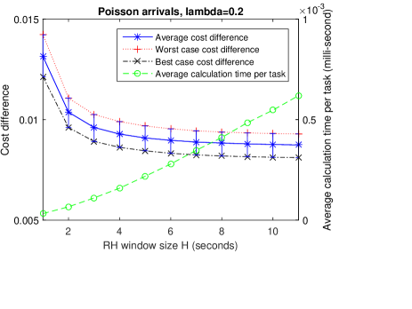
Figure 2: Simulation Results of Poisson Arrivals

.

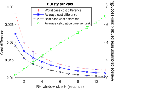
Figure 3: Simulation Results of Bursty Arrivals

In Fig. 2, we consider Poisson arrivals with $\lambda=0.2$. With RH window size $H$ varying from $1s$ to $11s$, the cost differences are well below $2\%$. When $H$ becomes larger, the cost differences are reduced; the calculation time per task increases since at each decision point, the optimization problem involves more tasks.

In the next experiment shown in Fig. 3, we consider bursty arrivals with the burst interval uniformly distributed over $[8,12]s$, the number of tasks in each burst chosen from $\{10,\ldots,20\}$ with equal probability, and the task intervals within the same burst uniformly distributed within $[0,1]$. Although the cost differences are just slightly higher than those in the Poisson case, the average calculation time per task is now much larger. This is because in the bursty arrival case, a large number of backlogged tasks are involved at each decision point.

Our simulation results show that the proposed RH control mechanism can not only guarantee feasibility when the off-line problem is feasible, but also achieve near optimal solutions.

V Conclusions

In this paper, we first study the Downlink Transmission Scheduling (DTS) problem. A simpler version of this problem has been studied in [2] and [9], where the MoveRight algorithm is proposed. The MoveRight algorithm is an iterative algorithm, and its rate of convergence is obtainable only when the cost function is not task-dependent. Compared with the work in [9] and [2], we deal with a much harder problem: i) our cost function is task-dependent and ii) each task has its own arrival time and deadline. This is essentially a hard convex optimization problem with nondifferentiable constraints. By analyzing the special structure of the optimal sample path, an efficient algorithm, known as the Generalized Critical Task Decomposition Algorithm (GCTDA), is proposed to solve the problem. Simulation results show that our algorithm is more appropriate for real-time applications than the MoveRight algorithm. Finally, we show that our results can be used in on-line control to achieve near optimal solutions for Poisson and bursty arrivals.

APPENDIX

Proof of Lemma III.3: Since $\omega_{i}(\tau)$ is strictly convex and differentiable,

$$v_{1}\omega_{1}(\tau_{1})-v_{1}\omega_{1}(\tau_{1}^{{}^{\prime}})>v_{1}(\tau_{1}-\tau_{1}^{{}^{\prime}})\dot{\omega}_{1}(\tau_{1}^{{}^{\prime}})$$ (24)

$$v_{2}\omega_{2}(\tau_{2})-v_{2}\omega_{2}(\tau_{2}^{{}^{\prime}})>v_{2}(\tau_{2}-\tau_{2}^{{}^{\prime}})\dot{\omega}_{2}(\tau_{2}^{{}^{\prime}})$$ (25)

Because $v_{1}\tau_{1}+v_{2}\tau_{2}=v_{1}\tau_{1}^{{}^{\prime}}+v_{2}\tau_{2}^{{}^{\prime}},$

$$v_{1}(\tau_{1}-\tau_{1}^{{}^{\prime}})=-v_{2}(\tau_{2}-\tau_{2}^{{}^{\prime}})=C>0$$ (26)

Summing (24) and (25) above, and using (26), we get:

$$v_{1}\omega_{1}(\tau_{1})+v_{2}\omega_{2}(\tau_{2})-v_{1}\omega_{1}(\tau_{1}^{{}^{\prime}})-v_{2}\omega_{2}(\tau_{2}^{{}^{\prime}})>$$

$$C(\dot{\omega}_{1}(\tau_{1}^{{}^{\prime}})-\dot{\omega}_{2}(\tau_{2}^{{}^{\prime}}))$$

Since $C>0$, and by assumption, $\dot{\omega}_{1}(\tau_{1}^{{}^{\prime}})-\dot{\omega}_{2}(\tau_{2}^{{}^{\prime}})>0,$

$$v_{1}\omega_{1}(\tau_{1})+v_{2}\omega_{2}(\tau_{2})>v_{1}\omega_{1}(\tau_{1}^{{}^{\prime}})+v_{2}\omega_{2}(\tau_{2}^{{}^{\prime}}).\text{ }{\small\blacksquare}$$

Proof of Lemma III.4: We only prove part (i). Part (ii) can be proved similarly. Let $\tau_{k}^{{}^{\ast}},\ldots,\tau_{n}^{\ast}$ be the optimal solution. By the definition of a left-critical task, we have $\dot{\omega}_{i}(\tau_{i}^{\ast})>\dot{\omega}_{i+1}(\tau_{i+1}^{\ast}).$ Because tasks $i$ and $i+1$ are within a single BP, $x_{i}^{\ast}\geq a_{i+1}.$ Suppose $x_{i}^{\ast}>a_{i+1}.$ Consider a feasible solution $\tau_{k}^{{}^{\prime}},\ldots,\tau_{n}^{{}^{\prime}},$ $s.t.,$

$$\tau_{j}^{{}^{\prime}} =\tau_{j}^{{}^{\ast}},\text{ }j\neq i,\text{ }j\neq i+1,$$

$$\tau_{i}^{{}^{\prime}} <\tau_{i}^{\ast},\text{ }\tau_{i+1}^{{}^{\prime}}>\tau_{i+1}^{\ast},\text{ }\dot{\omega}_{i}(\tau_{i}^{{}^{\prime}})>\dot{\omega}_{i+1}(\tau_{i+1}^{{}^{\prime}})$$

Note that such a feasible solution always exists as long as $\tau_{i}^{{}^{\prime}}$ and $\tau_{i+1}^{{}^{\prime}}$ are arbitrarily close to $\tau_{i}^{\ast}$ and $\tau_{i+1}^{\ast}$ respectively. From Lemma III.3, we get:

$$v_{i}\omega_{i}(\tau_{i}^{\ast})+v_{i+1}\omega_{i+1}(\tau_{i+1}^{\ast})>v_{i}\omega_{i}(\tau_{i}^{{}^{\prime}})+v_{i+1}\omega_{i}(\tau_{i+1}^{{}^{\prime}}).$$

Since $\tau_{j}^{{}^{\prime}}=\tau_{j}^{{}^{\ast}},$ $j\neq i,$ $j\neq i+1,$ using the above inequality, we get:

$$\sum_{i=k}^{n}v_{i}\omega_{i}(\tau_{i}^{\ast})>\sum_{i=k}^{n}v_{i}\omega_{i}(\tau_{i}^{{}^{\prime}}),$$

which contradicts the assumption that $\tau_{k}^{{}^{\ast}},\ldots,\tau_{n}^{\ast}$ is the optimal solution. Therefore, $x_{i}^{\ast}=a_{i+1}.$ ${\small\blacksquare}$

Proof of Lemma III.5: (i) Since $\omega_{m}(\tau)$ is strictly convex, continuous and differentiable, $\dot{\omega}_{m}(\tau)$ is also continuous. $NE(i,j;t_{1},t_{2})$ has a feasible solution, because $\dot{\omega}_{m}(\tau)$ is continuous and monotonically increasing, and $\tau$ can take any value in $(0,\infty).$ Now, suppose there are two different solutions to $NE(i,j;t_{1},t_{2}):\tau_{i}(t_{1},t_{2}),\ldots,\tau_{j}(t_{1},t_{2})$ and $\tau_{i}^{{}^{\prime}}(t_{1},t_{2}),\ldots,\tau_{j}^{{}^{\prime}}(t_{1},t_{2}).$ Then, the common derivatives of these two solutions are different. Without loss of generality, we assume $\sigma_{i,j}(t_{1},t_{2})>\sigma_{i,j}^{{}^{\prime}}(t_{1},t_{2}),$ which means $\dot{\omega}_{m}(\tau_{m}(t_{1},t_{2}))>\dot{\omega}_{m}(\tau_{m}^{{}^{\prime}}(t_{1},t_{2})),$ for any $m$, $i\leq m\leq j.$ By the convexity of $\omega_{m}(\tau)$, we obtain $\tau_{m}(t_{1},t_{2})>\tau_{m}^{{}^{\prime}}(t_{1},t_{2}),$ for any $m$, $i\leq m\leq j,$ and

$$\sum_{m=i}^{j}\tau_{m}(t_{1},t_{2})v_{m} =t_{2}-t_{1}>$$

$$\sum_{m=i}^{j}\tau_{m}^{{}^{\prime}}(t_{1},t_{2})v_{m} =t_{2}-t_{1},$$

which is a contradiction. Therefore, $NE(i,j;t_{1},t_{2})$ has a unique solution.

(ii) Let $\sigma_{i,j}(t_{1},t_{2})$, $\sigma_{i,j}(t_{3},t_{4})$ be the common derivative of $NE(i,j;$ $t_{1},t_{2})$ and $NE(i,j;t_{3},t_{4})$ respectively, $0<\Delta=t_{2}-t_{1}<\Delta^{{}^{\prime}}=t_{4}-t_{3}.$ Let $\tau_{i}(t_{1},t_{2}),\ldots,\tau_{j}(t_{1},t_{2})$, $\tau_{i}(t_{3},t_{4}),\ldots,\tau_{j}(t_{3},t_{4})$ be the solution to $NE(i,j;t_{1},t_{2})$ and $NE(i,j;t_{3},t_{4})$ respectively. We need to show $\sigma_{i,j}(t_{1},t_{2})<$ $\sigma_{i,j}(t_{3},t_{4}).$ Suppose $\sigma_{i,j}(t_{1},t_{2})\geq\sigma_{i,j}(t_{3},t_{4}).$ Then, by definition, we get $\dot{\omega}_{m}(\tau_{m}(t_{1},t_{2}))\geq\dot{\omega}_{m}(\tau_{m}(t_{3},t_{4})),$ for any $m$, $i\leq m\leq j.$ By the convexity of $\omega_{m}(\tau)$, $\tau_{m}(t_{1},t_{2})\geq\tau_{m}(t_{3},t_{4}),$ $i\leq m\leq j.$ Therefore,

$$\sum_{m=i}^{j}\tau_{m}(t_{1},t_{2})v_{m} =t_{2}-t_{1}=\Delta\geq$$

$$\sum_{m=i}^{j}\tau_{m}(t_{3},t_{4})v_{m} =t_{4}-t_{3}=\Delta^{{}^{\prime}}$$

which contradicts our assumption that $\Delta<\Delta^{{}^{\prime}}.$ Therefore, the common derivative of $NE(i,j;t_{1},t_{2})$ is a monotonically increasing function of $\Delta=t_{2}-t_{1}.$

(iii) It can be easily checked that $\tau_{i}(t_{1},t_{2}),\ldots,$ $\tau_{p}(t_{1},t_{2})$ and $\tau_{p+1}(t_{1},$ $t_{2}),\ldots,\tau_{j}(t_{1},$ $t_{2})$ are the unique solutions to $NE(i,p;t_{1},t_{1}+S_{ip})$ and $NE(p+1,j;t_{1}+S_{ip},t_{2})$ respectively. Therefore, by the definition of $NE(i,j;t_{1},t_{2})$ and $\sigma_{i,j}(t_{1},t_{2}),$ we have $\sigma_{i,p}(t_{1},t_{1}+S_{ip})=\sigma_{i,j}(t_{1},t_{2})$ and $\sigma_{p+1,j}(t_{1}+S_{ip},t_{2})=\sigma_{i,j}(t_{1},t_{2})$, which implies $\sigma_{i,p}(t_{1},t_{1}+S_{ip})=\sigma_{p+1,j}(t_{1}+S_{ip},t_{2})=\sigma_{i,j}(t_{1},t_{2}).$

(iv) Let $S_{ip}$ be the same as in (iii). By assumption, $c_{q}\neq c_{r}$ $\forall q,r\in\{1,2,3\},q\neq r.$ This implies that $t_{3}\neq S_{ip},$ otherwise $c_{q}=c_{r}.$ From the monotonicity of $\sigma_{i,j}(t_{1},t_{2})$ shown in part (ii), we get $\min(c_{1},c_{2})<c_{3}<\max(c_{1},c_{2}).$ ${\small\blacksquare}$

Proof of Lemma III.6: Invoking Lemma III.4, we get $x_{r}^{\ast}=d_{r}.$ Suppose there are left-critical tasks in $\{k,\ldots,r-1\}$ and the closest left-critical task to $r$ is task $l$, $k\leq l<r.$ Invoking Lemma III.4, $x_{l}^{\ast}=a_{l+1}.$ By assumption,

$$\sigma_{k,L_{r}}(a_{k},a_{L_{r}+1})\leq\sigma_{k,r}(a_{k},d_{r}).$$ (27)

Because $l<r,$ from (11),

$$\sigma_{k,l}(a_{k},a_{l+1})\leq\sigma_{k,L_{r}}(a_{k},a_{L_{r}+1}).$$ (28)

From (27) and (28), the following must be true:

$$\sigma_{k,l}(a_{k},a_{l+1})\leq\sigma_{k,r}(a_{k},d_{r})$$ (29)

When the equality holds in (29), from (iii) of Lemma III.5, we get

$$\sigma_{l+1,r}(a_{l+1},d_{r})=\sigma_{k,l}(a_{k},a_{l+1}).$$ (30)

When the inequality holds in (29), from (iv) of Lemma III.5, we obtain

$$\sigma_{l+1,r}(a_{l+1},d_{r})>\sigma_{k,r}(a_{k},d_{r}).$$

From (29) and the above inequality, we get

$$\sigma_{l+1,r}(a_{l+1},d_{r})>\sigma_{k,l}(a_{k},a_{l+1}).$$ (31)

Combining (30) and (31), we get

$$\sigma_{l+1,r}(a_{l+1},d_{r})\geq\sigma_{k,l}(a_{k},a_{l+1})$$ (32)

Since there is no right-critical or left-critical task in $\{l+1,\ldots,r-1\}$, invoking Lemma III.1, we get

$$\dot{\omega}_{s}(\tau_{s}^{\ast}) =\dot{\omega}_{s+1}(\tau_{s+1}^{\ast})=\sigma_{l+1,r}(a_{l+1},d_{r}),\text{ }$$

$$\forall s \in\{l+1,\ldots,r-1\}.$$

From the definition of left-critical tasks, we get

$$\dot{\omega}_{l}(\tau_{l}^{\ast})>\dot{\omega}_{l+1}(\tau_{l+1}^{\ast})=\sigma_{l+1,r}(a_{l+1},d_{r}).$$ (33)

We consider two cases:

Case 1: $k=l$. Then, $\sigma_{k,l}(a_{k},a_{l+1})=\dot{\omega}_{l}(\tau_{l}^{\ast}).$ Inequalities (32) and (33) contradict each other.

Case 2: $k<l$. We will use a contradiction argument to show that there must exist a right-critical task $m$, $k\leq m<l$, i.e.,

$$\dot{\omega}_{m}(\tau_{m}^{\ast})<\dot{\omega}_{m+1}(\tau_{m+1}^{\ast}).$$

Suppose such a task $m$ does not exist. i.e.,

$$\dot{\omega}_{m}(\tau_{m}^{\ast})\geq\dot{\omega}_{m+1}(\tau_{m+1}^{\ast}),\text{ }k\leq m<l.$$ (34)

Let

$$y_{m}=\left\{\begin{array}[]{ll}a_{k},&m=k-1\\ x_{m}^{\ast}&m=k,\ldots,l.\end{array}\right.$$

Inequality (34) is equivalent to the following:

$$\sigma_{m,m}(y_{m-1},y_{m}) \geq\sigma_{m+1,m+1}(y_{m},y_{m+1}),\text{ }$$ (35)

$$\text{for }m =k,\ldots,l-1.$$

We will use a recursive proof next:

Step 1: Letting $m=k$ in (35), we have

$$\sigma_{k,k}(y_{k-1},y_{k})\geq\sigma_{k+1,k+1}(y_{k},y_{k+1}).$$ (36)

When the equality holds in (36), invoking part (iii) of Lemma III.5, we get

$$\sigma_{k,k+1}(y_{k-1},y_{k+1})=\sigma_{k+1,k+1}(y_{k},y_{k+1}).$$ (37)

When the inequality holds in (36), invoking part (iv) of Lemma III.5, we get

$$\sigma_{k,k+1}(y_{k-1},y_{k+1})>\sigma_{k+1,k+1}(y_{k},y_{k+1}).$$ (38)

Combining (37) and (38) above, we have

$$\sigma_{k,k+1}(y_{k-1},y_{k+1})\geq\sigma_{k+1,k+1}(y_{k},y_{k+1}).$$ (39)

Step 2: Letting $m=k+1$ in (35), we have

$$\sigma_{k+1,k+1}(y_{k},y_{k+1})\geq\sigma_{k+2,k+2}(y_{k+1},y_{k+2}).$$

Combining (39) and the above inequality, we obtain

$$\sigma_{k,k+1}(y_{k-1},y_{k+1})\geq\sigma_{k+2,k+2}(y_{k+1},y_{k+2}).$$

Similarly to the derivation of (37), (38), and (39), we can get

$$\sigma_{k,k+2}(y_{k-1},y_{k+2})\geq\sigma_{k+2,k+2}(y_{k+1},y_{k+2}).$$

Repeating the process up to step $l-k,$ we obtain

$$\sigma_{k,l}(y_{k-1},y_{l})\geq\sigma_{l,l}(y_{l-1},y_{l}).$$

Since task $l$ is left-critical, from the definition of $y_{m}$ and Lemma III.4, $y_{l}=x_{l}^{\ast}=a_{l+1},$ and the above inequality is equivalent to

$$\sigma_{k,l}(a_{k},a_{l+1})\geq\dot{\omega}_{l}(\tau_{l}^{\ast}).$$ (40)

From (40) and (33), we get

$$\sigma_{k,l}(a_{k},a_{l+1})>\sigma_{l+1,r}(a_{l+1},d_{r}).$$

Invoking (iv) of Lemma III.5, we obtain

$$\sigma_{k,l}(a_{k},a_{l+1})>\sigma_{k,r}(a_{k},d_{r})$$

which contradicts (29). Therefore, there must exist a task $m$, $k\leq m<l$, s.t.,

$$\dot{\omega}_{m}(\tau_{m}^{\ast})<\dot{\omega}_{m+1}(\tau_{m+1}^{\ast})$$

By Definition 1, task $m$ is a right-critical task, which contradicts our assumption that task $r$ is the first right-critical task in $\{k,\ldots,n\}.$ Therefore, there is no left-critical task before task $r.$ ${\small\blacksquare}$

Proof of Lemma III.7: We use a contradiction argument to prove the lemma. Suppose there are right-critical tasks before task $R_{i}$ and the one with smallest index is task $r$, $k\leq r<R_{i}.$ By assumption, $\sigma_{k,j}(a_{k},d_{j})\geq\sigma_{k,L_{j}}(a_{k},a_{L_{j}+1}),$ for all $j$, $k<j<i.$ When $r>k$, letting $j=r$, we have $\sigma_{k,r}(a_{k},d_{r})\geq\sigma_{k,L_{r}}(a_{k},a_{L_{r}+1}).$ Then we can invoke Lemma III.6 to establish that there is no left-critical task in $\{k,\ldots,r-1\}$. Since there is also no right-critical task in $\{k,\ldots,r-1\},$ from Lemma III.1,

$$\dot{\omega}_{s}(\tau_{s}^{\ast})=\sigma_{k,r}(a_{k},d_{r}),\text{ }\forall s\in\{k,\ldots,r\}.$$ (41)

Since $k\leq r<R_{i},$ from (10), we have

$$\sigma_{k,R_{i}}(a_{k},d_{R_{i}})\leq\sigma_{k,r}(a_{k},d_{r}).$$ (42)

Then, from (ii) of Lemma III.5,

$$\sigma_{k,R_{i}}(a_{k},x_{R_{i}}^{\ast})\leq\sigma_{k,R_{i}}(a_{k},d_{R_{i}}).$$ (43)

Combining (42) and (43), we get

$$\sigma_{k,R_{i}}(a_{k},x_{R_{i}}^{\ast})\leq\sigma_{k,r}(a_{k},d_{r}).$$ (44)

Since $r$ is right-critical, from (41) and Definition 1,

$$\sigma_{k,r}(a_{k},d_{r})=\dot{\omega}_{r}(\tau_{r}^{\ast})<\dot{\omega}_{r+1}(\tau_{r+1}^{\ast}).$$ (45)

From (44) and (45), there must exist at least one left-critical task in $\{r+1,\ldots,R_{i}-1\};$ otherwise, from the definition of a left-critical task in Definition 1 and a simple contradiction argument, we have $\dot{\omega}_{s}(\tau_{s}^{\ast})\leq\dot{\omega}_{s+1}(\tau_{s+1}^{\ast}),\forall s\in\{r+1,\ldots,R_{i}-1\}.$ Using this result, (45) and a similar method as in obtaining (40), we can get $\sigma_{k,r}(a_{k},d_{r})<\sigma_{k,R_{i}}(a_{k},x_{R_{i}}^{\ast}),$ which contradicts (44).

Let the left-critical task with smallest index be $l.$ From Lemma III.4, $x_{l}^{\ast}=a_{l+1}.$ Similar to obtaining $\sigma_{k,r}(a_{k},d_{r})<\sigma_{k,R_{i}}(a_{k},x_{R_{i}}^{\ast})$ above, we can get

$$\sigma_{k,r}(a_{k},d_{r})<\sigma_{k,l}(a_{k},x_{l}^{\ast})=\sigma_{k,l}(a_{k},a_{l+1}).$$ (46)

By assumption, $\sigma_{k,j}(a_{k},a_{j+1})\leq\sigma_{k,R_{j}}(a_{k},d_{R_{j}}),$ and setting $j=l$, we get

$$\sigma_{k,l}(a_{k},a_{l+1})\leq\sigma_{k,R_{l}}(a_{k},d_{R_{l}}).$$

Since, from (10), we have $\sigma_{k,R_{l}}(a_{k},d_{R_{l}})\leq\sigma_{k,r}(a_{k},d_{r}),$ combining this and the above inequality, we obtain

$$\sigma_{k,l}(a_{k},a_{l+1})\leq\sigma_{k,r}(a_{k},d_{r})$$

which contradicts (46) and completes the proof. ${\small\blacksquare}$

Proof of Lemma III.8: Suppose task $R_{i}$ is not right-critical. By assumption,

$$\sigma_{k,R_{i}}(a_{k},d_{R_{i}})<\sigma_{k,i}(a_{k},a_{i+1}),$$

Because $x_{R_{i}}^{\ast}\leq d_{R_{i}},$ from (ii) of Lemma III.5,

$$\sigma_{k,R_{i}}(a_{k},x_{R_{i}}^{\ast})\leq\sigma_{k,R_{i}}(a_{k},d_{R_{i}}).$$ (47)

From the two inequalities above, we obtain:

$$\sigma_{k,R_{i}}(a_{k},x_{R_{i}}^{\ast})<\sigma_{k,i}(a_{k},a_{i+1}).$$ (48)

Invoking Lemma III.7, there is no right-critical task before task $R_{i}.$ Next, we use a contradiction argument to show that there must exist at least one right-critical task in $\{R_{i},\ldots,i-1\}$. Suppose there is no right-critical task in $\{R_{i},\ldots,i-1\}$. Because there is no right-critical task in $\{k,\ldots,i-1\}$, by Definition 1, we have

$$\dot{\omega}_{m}(\tau_{m}^{\ast})\geq\dot{\omega}_{m+1}(\tau_{m+1}^{\ast}),\text{ }m=k,\ldots,i-1.$$

Let

$$y_{m}=\left\{\begin{array}[]{ll}a_{k},&m=k-1\\ x_{m}^{\ast},&m=k,\ldots,i-1\\ a_{i+1},&m=i\end{array}\right.$$

The above inequality can be rewritten as

$$\sigma_{m,m}(y_{m-1},y_{m})\geq\sigma_{m+1,m+1}(y_{m},y_{m+1}),$$

$$\text{ }m=k,\ldots,i-1.$$

Similar to the way of obtaining (40) in proving Lemma III.6, we obtain

$$\sigma_{k,R_{i}}(a_{k},x_{R_{i}}^{\ast})\geq\sigma_{k,i}(a_{k},a_{i+1}),$$

which contradicts (48).

We showed there must exist at least one right-critical task in $\{R_{i},\ldots,i-1\}.$ From the initial contradiction assumption, $R_{i}$ is not right-critical. When $i=R_{i}+1,$ the contradiction proof is completed. Next, we consider the case when $i>R_{i}+1.$

Let $r$ be the closest right-critical task to $R_{i}$ in $\{R_{i},\ldots,i-1\}$. Since there is no right-critical task in $\{k,\ldots,r-1\},$ by Definition 1,

$$\dot{\omega}_{m}(\tau_{m}^{\ast})\geq\dot{\omega}_{m+1}(\tau_{m+1}^{\ast}),\text{ }m=k,\ldots,r-1.$$

Let

$$y_{m}=\left\{\begin{array}[]{ll}a_{k},&m=k-1\\ x_{m}^{\ast},&m=k,\ldots,r\end{array}\right.$$

The above inequality can be rewritten as

$$\sigma_{m,m}(y_{m-1},y_{m})\geq\sigma_{m+1,m+1}(y_{m},y_{m+1}),$$

$$\text{ }m=k,\ldots,r-1.$$

Similar to the way of obtaining (40) in proving Lemma III.6, we obtain

$$\sigma_{k,R_{i}}(a_{k},x_{R_{i}}^{\ast})\geq\sigma_{k,r}(a_{k},x_{r}^{\ast})=\sigma_{k,r}(a_{k},d_{r}).$$

From the above inequality and (47), we obtain

$$\sigma_{k,r}(a_{k},d_{r})\leq\sigma_{k,R_{i}}(a_{k},d_{R_{i}})$$

which contradicts the definition of $R_{i}$ in (6), since $R_{i}<r<i.$ Therefore, task $R_{i}$ must be right-critical. ${\small\blacksquare}$

Proof of Theorem III.1: We only prove part (i). Part (ii) can be proven similarly. The proof contains several steps: 1) using (12), Lemma III.6, and setting $j=R_{i},$ we conclude that there is no left-critical task before $R_{i};$ 2) using (12), (13), and Lemma III.7, we establish that there is no right-critical task before $R_{i};$ 3) using (12), (13), (14), and Lemma III.8, it follows that $R_{i}$ is a right-critical task; and finally 4) combining the results established in the previous steps 1)-3), we can obtain that $R_{i}$ is the first critical task in $\{k,\ldots,n\}$, and it is right-critical. ${\small\blacksquare}$

Justifications for Assumption 2: We only justify Part a). Part b) can be justified similarly. Using Shannon’s theorem, $\tau_{i}$ can be represented by the following equation:

$$\tau_{i}=\frac{1}{B\log_{2}(1+\frac{s_{i}P}{N_{0}})}$$

where $B$ is the bandwidth of the channel, $s_{i}$ is the task-dependent channel gain, $P$ is the transmission power, and $N_{0}$ is the power of the noise. Since $\frac{s_{i}P}{N_{0}}\gg 1$ in typical scenarios, we can omit the $1$ above and represent $P$ in terms of $\tau_{i}:$

$$P(\tau_{i})=\frac{N_{0}(2^{\frac{1}{B\tau_{i}}})}{s_{i}}$$ (49)

We assume that the maximum transmission power of each task is constant $P_{\max}$, and it determines $\tau_{i\_\min}$:

$$P_{\max}=\frac{N_{0}(2^{\frac{1}{B\tau_{i\_\min}}})}{s_{i}}$$ (50)

Because

$$\omega_{i}(\tau_{i})=P(\tau_{i})\tau_{i},$$

we use (49) and (50) to get

$$\dot{\omega}_{i}(\tau_{i})=P(\tau_{i})(1-\frac{1}{B\tau_{i}})=\frac{N_{0}(2^{\frac{1}{B\tau_{i}}})}{s_{i}}(1-\frac{1}{B\tau_{i}})$$ (51)

$$\dot{\omega}_{i}(\tau_{i})|_{\tau_{i}=\tau_{i\_\min}}=P_{\max}(1-\frac{1}{B\tau_{i\_\min}})$$ (52)

Using (52) and $\tau_{i\_\min}<\tau_{j\_\min},$ we have

$$\dot{\omega}_{i}(\tau_{i\_\min})<\dot{\omega}_{j}(\tau_{j\_\min}).$$

Using (50) and $\tau_{i\_\min}<\tau_{j\_\min}$, we get

$$s_{i}>s_{j},$$

i.e., the channel gain of task $i$ is greater than that of task $j$. Using (51), we get

$$\dot{\omega}_{i}(\tau)>\dot{\omega}_{j}(\tau).\text{ \ }{\small\blacksquare}$$

Proof of Lemma III.9: Let us assume that there exists tasks $\{p,\ldots,q\}$ $(k<p\leq q<n)$ in a BP $\{k,\ldots,n\}$ of the optimal sample path of $Q(k,n)$ such that

$$\tau_{p-1}^{\ast} \geq \tau_{p-1\_\min},\text{ }\tau_{q+1}^{\ast}\geq\tau_{q+1\_\min},\text{ }$$ (53)

$$\tau_{i}^{\ast} < \tau_{\min},\text{ }i=p,\ldots,q$$

From Assumption 1,

$$\dot{\omega}_{p-1}(\tau_{p-1}^{\ast}) \geq \dot{\omega}_{p-1}(\tau_{p-1\_\min}),\text{ }$$ (54)

$$\dot{\omega}_{q+1}(\tau_{q+1}^{\ast}) \geq \dot{\omega}_{q+1}(\tau_{q+1\_\min})$$

Let

$$z=\underset{i=k,\ldots,n}{\arg\min}\text{ }\tau_{i\_\min}.$$

Because $\tau_{i\_\min}\geq\tau_{z\_\min},$ we invoke Assumption 2 and get

$$\dot{\omega}_{i}(\tau_{\min})\leq\dot{\omega}_{z}(\tau_{\min}),\text{ }i=p,\ldots,q$$ (55)

From Assumption 1 and (53), we have

$$\dot{\omega}_{i}(\tau_{i}^{\ast})<\dot{\omega}_{i}(\tau_{\min}),\text{ }i=p,\ldots,q$$ (56)

Combine (55) and (56) above, we have

$$\dot{\omega}_{i}(\tau_{i}^{\ast})<\dot{\omega}_{z}(\tau_{\min}),\text{ }i=p,\ldots,q$$ (57)

Because $\tau_{p-1\_\min}\geq\tau_{\min}$, we invoke Assumption 2 and get

$$\dot{\omega}_{p-1}(\tau_{p-1\_\min})\geq\dot{\omega}_{z}(\tau_{\min})$$ (58)

Similarly, we use $\tau_{q+1\_\min}\geq\tau_{\min}$ and Assumption 2 to get

$$\dot{\omega}_{q+1}(\tau_{q+1\_\min})\geq\dot{\omega}_{z}(\tau_{\min})$$ (59)

Combining (54), (58), and (59), we have

$$\dot{\omega}_{p-1}(\tau_{p-1}^{\ast})\geq\dot{\omega}_{z}(\tau_{\min})\text{ and }\dot{\omega}_{q+1}(\tau_{q+1}^{\ast})\geq\dot{\omega}_{z}(\tau_{\min}).$$ (60)

Then, we combine (57) and (60) to get

$$\dot{\omega}_{p-1}(\tau_{p-1}^{\ast}) > \dot{\omega}_{i}(\tau_{i}^{\ast})\text{ and }\dot{\omega}_{i}(\tau_{i}^{\ast})<\dot{\omega}_{q+1}(\tau_{q+1}^{\ast}),\text{ }$$

$$i = p,\ldots,q.$$

From the inequalities above, we have

$$\dot{\omega}_{p-1}(\tau_{p-1}^{\ast})>\dot{\omega}_{p}(\tau_{p}^{\ast})\text{ and }\dot{\omega}_{q}(\tau_{q}^{\ast})<\dot{\omega}_{q+1}(\tau_{q+1}^{\ast}).$$

Invoking Lemma III.4, we have

$$x_{p-1}^{\ast}=a_{p}\text{ and }x_{q}^{\ast}=d_{q}.$$ (61)

Because $x_{q}^{\ast}=x_{p-1}^{\ast}+\sum_{i=p}^{q}v_{i}\tau_{i}^{\ast},$ we use (53) and (61) to get:

$$x_{q}^{\ast}-x_{p-1}^{\ast} = d_{q}-a_{p}=\sum_{i=p}^{q}v_{i}\tau_{i}^{\ast}$$

$$< \sum_{i=p}^{q}v_{i}\tau_{\min}\leq\sum_{i=p}^{q}v_{i}\tau_{i\_\min}$$

For any feasible solution of $Q^{\prime}(k,n),$ we must have

$$\sum_{i=p}^{q}v_{i}\tau_{i}^{\prime}\leq d_{q}-a_{p}\leq\sum_{i=p}^{q}v_{i}\tau_{i\_\min},$$

which implies that there exists at least one $\tau_{i}^{\prime},i=p,\ldots,q$, such that $\tau_{i}^{\prime}<\tau_{i\_\min}.$ This completes the proof that $Q^{\prime}(k,n)$ is infeasible. ${\small\blacksquare}$

Proof of Theorem IV.1: Because P2 is feasible, we have

$$x_{i}^{{}^{\prime}\ast}\leq d_{i}.$$

To prove the theorem, we only need to show that $\tilde{x}_{i}\leq x_{i}^{{}^{\prime}\ast}$ for $i=1,\ldots,N.$ We use induction to prove it.

1) When $t=0$, we are at the first decision point $\tilde{x}_{0}=a_{1}.$ We have two cases:

Case 1.1: We apply $\tau_{1\_\min}$ to task 1. It is obvious that $\tilde{x}_{1}\leq x_{i}^{{}^{\prime}\ast}.$

Case 1.2: We apply control $\widetilde{\tau}_{1}^{\ast}$ obtained in either Step 1 or Step 2 of Table V to task 1. Without loss of generality, let us assume that $\widetilde{\tau}_{1}^{\ast}$ is obtained from Step 1 of Table V. In this case, $\widetilde{\tau}_{i}^{\ast},i=1,\ldots,h,$ are the solution to $\tilde{Q}(1,h)$ and $\widetilde{\tau}_{i}^{\ast}\geq\tau_{i\_\min}$ for all $i$. Therefore, $\widetilde{\tau}_{i}^{\ast}$ is also the solution to problem $\tilde{Q}^{\prime}(1,h).$ We have two subcases:

Case 1.2.1: When the planning horizon contains the end of a busy period on the optimal sample path, it is trivial that $\widetilde{\tau}_{1}^{\ast}=\tau_{1}^{{}^{\prime}\ast}.$ Therefore, $\tilde{x}_{1}=x_{1}^{\prime\ast}\leq d_{1}.$

Case 1.2.2: We now consider the more interesting case that $d_{i}\geq\widetilde{a}_{i+1},i=1,\ldots,h.$ To compare the RH problem and the off-line problem, we now add subscripts to indicate the starting and ending times of each problem. In particular, we use $\tilde{Q}_{a_{1},a_{1}+H}^{\prime}(1,h)$ to show that the starting transmission time of $\tilde{Q}^{\prime}(1,h)$ is $a_{1}$ and the ending transmission time is $a_{1}+H.$ Similarly, we use $Q_{a_{1},x_{h}^{\prime\ast}}^{\prime}(1,h)$ to show that the starting transmission time of $Q^{\prime}(1,h)$ is $a_{1}$ and the ending transmission time is $x_{h}^{{}^{\prime}\ast}.$ Because $a_{h+1}>a_{1}+H$ and $d_{h}\geq a_{1}+H,$ we must have $x_{h}^{{}^{\prime}\ast}\geq a_{1}+H.$ Looking at $\tilde{Q}_{a_{1},a_{1}+H}^{\prime}(1,h)$ and $Q_{a_{1},x_{h}^{\prime\ast}}^{\prime}(1,h),$ they are exactly the same, except that the ending transmission time of $Q_{a_{1},x_{h}^{\prime\ast}}^{\prime}(1,h)$ is potentially at a later time. Therefore, the optimal departure time of any task in $Q_{a_{1},x_{h}^{\prime\ast}}^{\prime}(1,h)$ must not be earlier than that in $\tilde{Q}_{a_{1},a_{1}+H}^{\prime}(1,h),$ which means $\tilde{x}_{1}\leq x_{1}^{\prime\ast}.$

2) Suppose that the RH controller is at decision point $\tilde{x}_{t}$, and $\tilde{x}_{t}\leq x_{t}^{\prime\ast}.$ We also have two cases:

Case 2.1: We apply $\tau_{t+1\min}$ to task $t+1$. It is obvious that $\tilde{x}_{t+1}\leq x_{t+1}^{\prime\ast}.$

Case 2.2: We apply control $\widetilde{\tau}_{t+1}^{\ast}$ obtained in either Step 1 or Step 2 of Table V to task 1. Without loss of generality, let us assume that $\widetilde{\tau}_{t+1}^{\ast}$ is obtained from Step 1 of Table V. In this case, $\widetilde{\tau}_{i}^{\ast},i=t+1,\ldots,h,$ are the solution to $\tilde{Q}(t+1,h)$ and $\widetilde{\tau}_{i}^{\ast}\geq\tau_{i\_\min}$ for all $i$. Therefore, $\widetilde{\tau}_{i}^{\ast}$ is also the solution to problem $\tilde{Q}^{\prime}(t+1,h).$ We consider two subcases:

Case 2.2.1: When the planning horizon contains the end of a busy period on the optimal sample path, i.e., there exists task $j\epsilon\{t+1,\ldots,h\}$ s.t. $d_{j}<\widetilde{a}_{j+1},$ we focus on tasks $\{t+1,\ldots,j\}.$ In this case, the controls of these tasks on the RH sample path are the solutions to problem $\tilde{Q}_{\tilde{x}_{t},d_{j}}^{\prime}(t+1,j)$, and the control of these tasks on the optimal sample path of P2 are the solutions to problem $Q_{x_{t}^{\prime\ast},d_{j}}^{\prime}(t+1,j).$ Looking at $\tilde{Q}_{\tilde{x}_{t},d_{j}}^{\prime}(t+1,j)$ and $Q_{x_{t}^{\prime\ast},d_{j}}^{\prime}(t+1,j)$, they are identical, except that the starting transmission time of $\tilde{Q}_{\tilde{x}_{t},d_{j}}^{\prime}(t+1,j)$ is potentially earlier than that of $Q_{x_{t}^{\prime\ast},d_{j}}^{\prime}(t+1,j).$ Therefore, the optimal departure time of any task in $\tilde{Q}_{\tilde{x}_{t},d_{j}}^{\prime}(t+1,j)$ must be no later than that in $Q_{x_{t}^{\prime\ast},d_{j}}^{\prime}(t+1,j),$ which means $\tilde{x}_{t+1}\leq x_{t+1}^{\prime\ast}.$

Case 2.2.2: $d_{i}\geq\widetilde{a}_{i+1},i=t+1,\ldots,h.$ In this case, the controls of tasks $\{t+1,\ldots,h\}$ on the RH sample path are the solutions to problem $\tilde{Q}_{\tilde{x}_{t},\tilde{x}_{t}+H}^{\prime}(t+1,h)$, and the control of these tasks on the optimal sample path of P2 are the solutions to problem $Q_{x_{t}^{\prime\ast},x_{h}^{\prime\ast}}^{\prime}(t+1,h).$ Because $a_{h+1}>\tilde{x}_{t}+H$ and $d_{h}\geq\tilde{x}_{t}+H,$ we must have $x_{h}^{{}^{\prime}\ast}\geq\tilde{x}_{t}+H.$ Looking at $\tilde{Q}_{\tilde{x}_{t},\tilde{x}_{t}+H}^{\prime}(t+1,h)$ and $Q_{x_{t}^{\prime\ast},x_{h}^{\prime\ast}}^{\prime}(t+1,h),$ they are exactly the same, except that both the starting and ending transmission times of $\tilde{Q}_{\tilde{x}_{t},\tilde{x}_{t}+H}^{\prime}(t+1,h)$ are potentially sooner than those of $Q_{x_{t}^{\prime\ast},x_{h}^{\prime\ast}}^{\prime}(t+1,h)$. Therefore, the optimal departure time of any task in $\tilde{Q}_{\tilde{x}_{t},\tilde{x}_{t}+H}^{\prime}(t+1,h)$ must be no later than that in $Q_{x_{t}^{\prime\ast},x_{h}^{\prime\ast}}^{\prime}(t+1,h),$ which means $\tilde{x}_{t+1}\leq x_{t+1}^{\prime\ast}.$ ${\small\blacksquare}$

References

- [1] T. D. Burd, T. A. Pering, A. J. Stratakos, and R. W. Brodersen, “A dynamic voltage scaled microprocessor system,” IEEE Journal of Solid-state Circuits, vol. 35, pp. 1571–1580, Nov. 2000.
- [2] A. E. Gamal, C. Nair, B. Prabhakar, E. Uysal-Biyikoglu, and S. Zahedi, “Energy-efficient scheduling of packet transmissions over wireless networks,” in Proceedings of IEEE INFOCOM, vol. 3, 23-27, New York City, USA, 2002, pp. 1773–1782.
- [3] C. E. Shannon and W. Weaver, The Mathematical Theory of Communication. Urbana, Illinois: University of Illinois Press, 1949.
- [4] B. E. Collins and R. L. Cruz, “Transmission policies for time varying channels with average delay constraints,” in Proceedings of Allerton Conference on Communications, Control, and Computing, Monticello, IL, 1999.
- [5] R. Berry, “Power and delay trade-offs in fading channels,” Ph.D. Dissertation, Massachusetts Institute of Technology, Cambridge, MA, 2000.
- [6] B. Ata, “Dynamic power control in a wireless static channel subject to a quality of service constraint,” Operations Research, vol. 53, 2005.
- [7] ——, “Dynamic power control in a wireless fading channel subject to a quality of service constraint,” submitted for publication.
- [8] M. Neely, “Energy optimal control for time varying wireless networks,” IEEE Trans. on Information Theory, vol. 52, pp. 2915 – 2934, 2006.
- [9] E. Uysal-Biyikoglu, B. Prabhakar, and A. E. Gamal, “Energy-efficient packet transmission over a wireless link,” IEEE/ACM Transactions on Networking, vol. 10, pp. 487–499, Aug. 2002.
- [10] M. Zafer and E. Modiano, “Minimum energy transmission over a wireless channel with deadline and power constraints,” IEEE Trans. on Automatic Control, vol. 54, pp. 2841 – 2852, 2009.
- [11] ——, “Delay-constrained energy efficient data transmission over a wireless fading channel,” in IEEE Information Theory and Applications Workshop, San Diego, CA, USA, Jan-Feb 2007.
- [12] ——, “Optimal rate control for delay-constrained data transmission over a wireless channel,” IEEE Trans. on Information Theory, vol. 54, pp. 4020 – 4039, 2008.
- [13] W. Chen, M. Neely, and U. Mitra, “Energy efficient scheduling with individual packet delay constraints: offline and online results,” in IEEE Infocom, Anchorage, Alaska, USA, May 2007.
- [14] W. Chen, U. Mitra, and M. Neely, “Energy-efficient scheduling with individual packet delay constraints over a fading channel,” ACM Wireless Networks, vol. 15, pp. 601–618, 2009.
- [15] M. Zafer and E. Modiano, “A calculus approach to energy-efficient data transmission with quality-of-service constraints,” IEEE/ACM Trans. on networking, vol. 17, pp. 898–911, 2009.
- [16] X. Wang and Z. Li, “Energy-efficient transmissions of bursty data packets with strict deadlines over time-varying wireless channels,” IEEE Trans. on Wireless Communications, vol. 12, pp. 2533–2543, 2013.
- [17] M. I. Poulakis, A. D. Panagopoulos, and P. Canstantinou, “Channel-aware opportunistic transmission scheduling for energy-efficient wireless links,” IEEE Trans. on Vehicular Technology, vol. 62, pp. 192–204, 2013.
- [18] Z. Zhou, P. Soldati, H. Zhang, and M. Johansson, “Energy-efficient deadline-constrained maximum reliability forwarding in lossy networks,” IEEE Trans. on Wireless Communications, vol. 11, pp. 3474–3483, 2012.
- [19] F. Shan, J. Luo, W. Wu, M. Li, and X. Shen, “Discrete rate scheduling for packets with individual deadlines in energy harvesting systems,” IEEE Journal on Selected Areas in Communications, vol. 33, pp. 438–451, 2015.
- [20] B. Tomasi and J. C. Preisig, “Energy-efficient transmission strategies for delay constrained traffic with limited feedback,” IEEE Trans. on Wireless Communications, vol. 14, pp. 1369–1379, 2015.
- [21] X. Zhong and C. Xu, “Online energy efficient packet scheduling with delay constraints in wireless networks,” in IEEE Infocom, Phoenix, AZ, April 2008.
- [22] R. Vaze, “Competitive ratio analysis of online algorithms to minimize packet transmission time in energy harvesting communication system,” in IEEE Infocom, Turin, April 2013.
- [23] L. Miao and C. G. Cassandras, “Optimal transmission scheduling for energy-efficient wireless networks,” in Proceedings of IEEE INFOCOM, Barcelona, Spain, 2006, pp. 1–11.
- [24] A. J. Goldsmith, “The capacity of downlink fading channels with variable rate and power,” IEEE Transactions on Information Theory, vol. 46, pp. 569–580, Aug 1997.
- [25] R. R. Kompella and A. C. Snoeren, “Practical lazy scheduling in sensor networks,” in Proceedings of the 1st International Conference on Embedded Networked Sensor Systems, Los Angeles, CA, 2003, pp. 280–291.
- [26] Y. C. Cho, C. G. Cassandras, and D. L. Pepyne, “Forward decomposition algorithms for optimal control of a class of hybrid systems,” International Journal of Robust and Nonlinear Control, vol. 11(5), pp. 497–513, 2001.
- [27] P. Zhang and C. G. Cassandras, “An improved forward algorithm for optimal control of a class of hybrid systems,” IEEE Trans. on Automatic Control, vol. 47, pp. 1735–1739, 2002.
- [28] L. Miao and C. G. Cassandras, “Optimality of static control policies in some discrete event systems,” IEEE Transactions on Automatic Control, vol. 50, pp. 1427–1431, Sep 2005.
- [29] J. Mao, C. G. Cassandras, and Q. Zhao, “Optimal dynamic voltage scaling in energy-limited nonpreemptive systems with real-time constraints,” IEEE Trans. on Mobile Computing, vol. 6, no. 6, pp. 678–688, 2007.
- [30] C. G. Cassandras and R. Mookherjee, “Receding horizon optimal control for some stochastic hybrid systems,” in Proceedings of the 42nd IEEE Conference on Decision and Control, vol. 3, Dec. 2003, pp. 2162–2167.
- [31] L. Miao and C. G. Cassandras, “Receding horizon control for a class of discrete-event systems with real-time constraints,” IEEE Transactions on Automatic Control, vol. 52, pp. 825–839, May 2007.