Stellar population synthesis based modelling of the Milky Way using asteroseismology of 13000 Kepler red giants.
Abstract
With current space-based missions it is now possible to obtain age-sensitive asteroseismic information for tens of thousands of red giants. This provides a promising opportunity to study the Galactic structure and evolution. We use asteroseismic data of red giants, observed by Kepler, to test the current theoretical framework of modelling the Galaxy based on population synthesis modeling and the use of asteroseismic scaling relations for giants. We use the open source code Galaxia to model the Milky Way and find the distribution of the masses predicted by Galaxia to be systematically offset with respect to the seismically-inferred observed masses. The Galactic model overestimates the number of low mass stars, and these stars are predominantly old and of low metallicity. Using corrections to the scaling relation suggested by stellar models significantly reduces the disagreement between predicted and observed masses. For a few cases where non-seismic mass estimates are available, the corrections to also improve the agreement between seismic and non-seismic mass estimates. The disagreement between predictions of the Galactic model and the observations is most pronounced for stars with and or for K. Altering the star formation rate in order to suppress stars older than 10 Gyr improves the agreement for mass but leads to inconsistent color distributions. We also tested the predictions of the TRILEGAL Galactic model. However, unlike Galaxia, it had difficulties in reproducing the photometric properties of the Kepler Input Catalog because it overestimates the number of blue stars. We conclude that either the scaling relations and/or the Galactic models need to be revised to reconcile predictions of theory with asteroseismic observations.
Subject headings:
Galaxy: disk – Galaxy: stellar content – Galaxy:structure – asteroseismology – stars: fundamental parameters1. Introduction
Our understanding of the formation of the Milky Way is seriously hampered by our inability to reliably measure ages of stars. In recent years, asteroseismology has been been demonstrated as a promising method to estimate fundamental stellar properties, including ages. From the seismology one can infer stellar radius and mass, and for red giants, mass is a good age indicator when the metallicity is known (Chaplin & Miglio, 2013). The fact that we can access asteroseismic information for a large number of stars, due to missions like Kepler (Hekker et al., 2011; Stello et al., 2013), CoRoT (Mosser et al., 2010; Miglio et al., 2013b), and now also K2 (Stello et al., 2015a), means that we can start using this information to unravel the formation history of the Milky Way.
We can use asteroseismic information to model the Milky Way within the framework of stellar population synthesis (Robin & Creze, 1986). Such models generate a synthetic catalog of stars for a given prescription of galactic structure and evolution. The predictions can then be directly compared to observations. A few such models are publicly available and have been developed and fine tuned to satisfy observational constraints from various photometric, spectroscopic, and astrometric surveys. These include Besançon (Robin et al., 2003), TRILEGAL (Girardi et al., 2005) and Galaxia (Sharma et al., 2011).
The first study to make use of asteroseismic information to test a stellar population synthesis-based model was performed by Miglio et al. (2009). A more comprehensive study was carried out by Chaplin et al. (2011), who compared the mass and radius distributions of about 400 main-sequence and subgiant stars with the TRILEGAL stellar population synthesis model (Girardi et al., 2005). They found that the radius distribution matched with the model predictions but the mass distribution showed significant differences. Specifically, the model was found to under predict the number of low mass stars (). However, the Kepler main-sequence/subgiant sample is small in size, is local to the Sun and is dominated by young stars, which limits it applicability for detailed model comparison.
In comparison to main-sequence and subgiant stars, red giants offer a number of advantages. For red giants the age is almost independent of luminosity. Hence, for any given apparent-magnitude-limited sample, one can obtain red giants spanning a wide range in age. Being luminous, they probe the Galaxy further for any given apparent magnitude and allow us to sample different regions of the Galaxy. The ability to sample different regions of the Galaxy is essential for Galactic archaeology because different regions of the Galaxy are dominated by different components. For example, the fraction of old stars increases with height above the Galactic mid plane.
Miglio et al. (2013b) carried out a differential study of the Milky Way using red giants with asteroseismic information from CoRoT. Using about 2000 red giants in two different regions of the Galaxy, they showed that the mass distributions differ, in agreement with theoretical models. However, they did not make a direct comparison with Galactic models. With Kepler, we now have a sample of oscillating red giants that is more than an order of magnitude larger than any other asteroseismic sample that has been tested against predictions of stellar population synthesis models (12964 red giants by Stello et al., 2013). The aim of this paper is to use this large sample of giants in the context of modeling the Galaxy.
However, a significant outstanding problem of using red giants is that modeling their individual frequencies is too time consuming for the analysis of tens of thousands of stars. We therefore rely on using asteroseismic scaling relations, and (Brown et al., 1991; Kjeldsen & Bedding, 1995), to estimate their radius and mass (and hence age). Here, is the frequency of maximum amplitude and the average large frequency separation. These relations assume that the structure of a red giant star is homologous with respect to the Sun. In reality this assumption is not strictly correct and verification of the relations is ongoing. However, independent high-precision estimates of mass and radius required for this verification are difficult to obtain. For subgiants and dwarfs, the scaling relation has been shown to work well (Bedding, 2014) and recently, Coelho et al. (2015) found the proportionality to be accurate to within 1.5%. Using Hipparcos parallaxes and/or interferometry, the asteroseismic radii calculated from scaling relations have been found to be accurate to within 5% (Bruntt et al., 2010; Silva Aguirre et al., 2012; Huber et al., 2012). For giants we generally do not have accurate parallaxes, so such studies are awaiting results from Gaia (Perryman, 2002). Open clusters have been used to test the scaling relations for giants (Brogaard et al., 2012; Sandquist et al., 2013; Miglio et al., 2012). Miglio et al. (2012) found agreement to within 5% for scaling relation-based radii. Testing of masses is more challenging. For a few cases where such verification have been performed, the scaling relation-based masses seem to be overestimated for giants (Miglio et al., 2012; Frandsen et al., 2013; Epstein et al., 2014). For two lower red giant branch stars (Epstein et al., 2014) find evidence that the mass estimated by using only (but with additional independent quantities) is lower compared to using both and . Based on this they suggested that a modification to the scaling relation might be required. Theoretical modelling has suggested corrections to the scaling relation (Stello et al., 2009; White et al., 2011; Miglio et al., 2013a), but there has been no comprehensive study to verify the corrections. In relation to , Houdek et al. (1999) and Chaplin et al. (2008) had suggested theoretically that coincides with the plateau of the damping rate with frequency. Belkacem et al. (2011) confirmed this for the Sun using SoHO GOLF observations. Balmforth (1992) suggested that this is caused by a resonance between the thermal adjustment time of the superadiabatic boundary layer and the mode frequency, which was also confirmed by the theoretical study of Belkacem et al. (2011) (see also Belkacem, 2012; Belkacem et al., 2013). However, there is currently no way to accurately predict from theory.
Additionally, there are a few factors related to the Kepler red giant sample that make it difficult to use them for population synthesis-based modeling. Firstly, knowing the selection function of the stellar sample is an essential requirement for such an analysis. However, this function has currently not been quantified. Secondly, the and band photometry in the Kepler Input Catalog (KIC, Brown et al., 2011) differs slightly from the corresponding Sloan magnitudes (Pinsonneault et al., 2012). This means the synthetic photometry that comes with isochrones, which is calibrated to Sloan magnitudes, needs to be re-calibrated, and this has not been done. We specifically address these issues here.
The paper is organized as follows. Section 2, describes our methods. We first describe the Galactic models that are compared against the seismic observations. Next, we discuss how to map the synthetic stars of Galactic models into the observational space. Following this, we discuss how to convert mass and radius to asteroseismic observables and vice verse. In Section 3, we analyze the Kepler giant samples. We investigate corrections to the scaling relations in Section 4, and corrections to the Galactic model in Section 5. Finally, in Section 6, we discuss implications of our findings.
2. Methods
2.1. Stellar-population-synthesis-based modeling of the Milky Way
The main Galactic stellar-population-synthesis model used in this paper is from the Galaxia code 111http://www.galaxia.sourceforge.net (Sharma et al., 2011). It uses a Galactic model based on the Besançon model by Robin et al. (2003) but with some modifications. Galaxia uses its own 3D extinction scheme to specify the dust distribution. We also apply a low latitude correction to the dust maps as in Sharma et al. (2014). The isochrones to predict the stellar properties are from the Padova database (Marigo et al., 2008; Bertelli et al., 1994). The unique feature of Galaxia is its novel star-spawning scheme which, unlike previous codes, does not discretize the spatial dimensions into multiple lines of sight. Instead, it generates a continuous three-dimensional distribution of stars.
Full details of the Galactic model are available in Robin et al. (2003) and Sharma et al. (2011), but here we summarize the main features. The Milky Way in Galaxia/Besançon consists of four major components: the thin disc, the thick disc, the bar shaped bulge, and the halo. Each component has its own initial mass function (IMF) and an analytic formula for the spatial distribution of stars. The thin disc is built up using a star-formation history, while other components are assumed to be populations of fixed age. In the thin disc, the metallicity of stars is governed by an age metallicity relation and the spatial distribution of stars is governed by an age scale-height relation. The full Besançon Galactic model is tuned to satisfy constraints from the Hipparcos mission (ESA, 1997) and star counts from surveys in optical and near infrared bands (Robin et al., 2003). The Galactic potential is computed in a self-consistent manner taking into account the results from the Hipparcos mission.
In addition to Galaxia, we used the TRILEGAL222http://stev.oapd.inaf.it/cgi-bin/trilegal Galactic stellar-population-synthesis model (Girardi et al., 2005). Unlike Galaxia, TRILEGAL cannot generate stars over a wide angular area. Therefore, we generated stars along 21 lines of sight pointing towards the centers of the 21 Kepler CCD-module foot prints on sky. We used TRILEGAL with the default settings but with binary stars turned off. For extinction, we used the extinction model of Galaxia. One noticeable difference between Galaxia and TRILEGAL is that, Galaxia uses a constant star formation rate, while the default setting in TRILEGAL uses a two-step star-formation rate, in which the rate between 1-4 Gyr is twice that at any other time.
2.1.1 Comparing the synthetic catalog photometry to the Kepler input catalog
Before we can start comparing the asteroseismic results with predictions from our Galactic models, we have to make sure that the photometry of stars in the KIC and the Galactic model predictions agree with each other. This is because the asteroseismic targets observed by Kepler were selected based on KIC parameters, which ultimately relied in its photometric entries. If the photometry of the Galactic model does not match with the KIC, the model will be fundamentally inconsistent with observations, preventing meaningful model-based inferences to be made. To proceed, we first compared the photometry of the synthetic stars with that of stars in the KIC and identified any differences. Next, we investigated the cause of any mismatch and derive transformation formulae to rectify it.
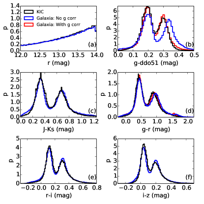
We generated a synthetic catalog of the Milky Way using the code Galaxia. Stars, both from the synthetic catalog and from the KIC, that lie within 8 degrees from the center of the Kepler field and with magnitude were selected for comparison. Note the KIC is expected to be complete to magnitudes even fainter than 14 magnitude in . We then added photometric errors to the stars. For this we derived the following formulas to approximate the actual photometric errors in 2MASS and the KIC (Figure 4 in Brown et al., 2011):
| (1) | |||||
| (2) |
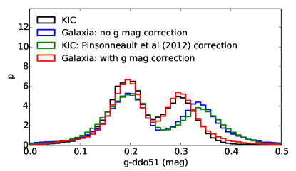
In LABEL:kic_photo1, we show the distribution of band magnitude and various colors for both the KIC (black) and the synthetic catalog (blue) 333In this paper we plot normalized distributions such that the integral over the abscissa is unity. This corresponds to probability density and is labelled as .. The magnitude and the color distributions match well, which is encouraging given that we do not enforce any fine tuning of the model. However, the distributions of and (LABEL:kic_photo1b,d) for the synthetic catalog are slightly redder for the giants (right most peaks). The discrepancy for is especially large. Either the band or the band photometry, or both could be discrepant. A clue to the cause of the discrepancy is provided by results of Pinsonneault et al. (2012), who found systematic differences in the KIC photometry with respect to SDSS photometry, for a small part of the Kepler field which overlaps with the SDSS. Because the isochrones that we use are calibrated to the SDSS bands, this could partly explain the mismatch that we see with the KIC. To investigate this, we show in LABEL:kic_photo2, a copy of LABEL:kic_photo1b, but we add (in green) the color after applying the Pinsonneault et al. (2012) transformations to the KIC stars. We see that this corrected KIC distribution matches the predictions of Galaxia (blue). Hence, a correction in band is enough to explain the mismatch seen in the distribution of color. The transformations proposed by Pinsonneault et al. (2012) were:
| (3) | ||||
A slight adjustment of zero-points (see square brackets) from the original Pinsonneault et al. (2012) transformations was needed to make the green curve match with the Galaxia prediction. Note slight adjustments of zero points are quite common when comparing photometry obtained from different sources.
The transformations of Pinsonneault et al. (2012) convert KIC photometry to SDSS. However, for our analysis we require the inverse transformation, that is from SDSS to KIC colors. This is because the stars observed by Kepler were selected from the KIC photometry and not a re-calibrated version of it. Equations 3 can be written in a matrix form and then inverted to get the transformation formula for , but this would require knowing the magnitudes in three bands and . Instead, for our use, we derived a simpler formula
| (4) |
that makes use of only two bands, and . The formula is easily invertible to . Moreover, because and are on different photometric systems, their errors are less likely to be correlated, which means the formula given by Equation 4 is more robust. The formula was derived by matching the distribution of synthetic stars to those in the KIC. The red curve in LABEL:kic_photo2 shows the results after applying Equation 4 to the band photometry of the synthetic catalog, which makes the color distribution of synthetic stars agree nicely with that of the KIC (black). This result is copied onto LABEL:kic_photo1b. The formula was also found to improve the agreement for the color distribution, which is shown in LABEL:kic_photo1d. Thus, we can now successfully reproduce the photometry of the KIC stars using Galaxia. For the rest of the paper we use the above formula to transform the band photometry of synthetic stars to compare the results of Galaxia with observations. In general, the formula should be valid for the version of Padova isochrones adopted in Galaxia. We note that Farmer et al. (2013) has also suggested transformations from SDSS to KIC photometry, but those transformations (like ours) are specific to the adopted stellar models and to the adopted bolometric corrections. We found their transformations to be inadequate to explain the mismatch of the color that we encounter.
2.2. Estimating KIC stellar parameters of stars in the synthetic catalog
As mentioned in the previous section, stellar targets of the Kepler mission were selected based on stellar parameters in the KIC, such as , and . These parameters were derived from photometry as part of the stellar classification project (hereafter SCP). As part of the SCP, Brown et al. (2011) developed a software code444https://www.cfa.harvard.edu/kepler/kic/kicindex.html to generate stellar parameters for the stars in the KIC based on a Bayesian posterior maximization scheme. In order to reproduce the selection function of the observed targets, we used this SCP software code to generate KIC-equivalent stellar parameters for stars in the synthetic catalog.
To run the SCP code, one has to specify the photometric bands to be used and the photometric uncertainty in each band. While the KIC contains photometry in 10 bands, we chose to use only the following eight that are available for the majority of stars. We set the photometric uncertainty to 0.005 which was found to best reproduce the KIC stellar parameters when applied to KIC stars. The adopted photometric uncertainty is close to but smaller than the quoted typical uncertainty in the KIC of mag for (Brown et al., 2011).
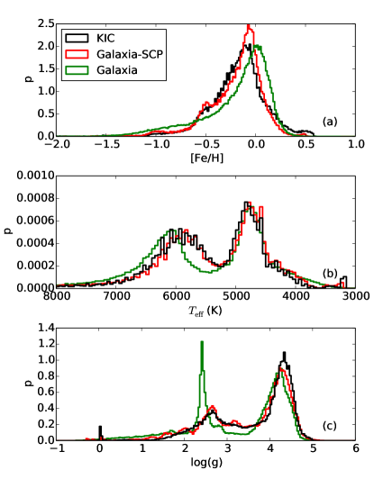
Finally, we checked if our population synthesis model can match the distribution of stellar parameters in the KIC. The comparison is shown in LABEL:kic_spc2. We see that the SCP-generated stellar parameters in the synthetic catalog (red line) match well with that of the KIC (black line), which is a prerequisite to reproduce the selection function of the Kepler mission. As an aside, we compared the true stellar parameters (green line) of the synthetic catalog with that of their SCP estimates (red line). We see slight differences. The SCP code underestimates by about 0.1 dex. The gravity of giants () is overestimated and also has significant uncertainty (red peak at is broadened and shifted). Finally, for stars hotter than 5200 K SCP underestimates by about 300 K. This means that the KIC underestimates the radii of the main sequence stars. A similar effect was also reported by Verner et al. (2011) while comparing the asteroseismic radii with the KIC radii for a sample of subgiants and dwarfs. The underestimation of radius by KIC, has important implcations for detecting planets in habitable zones around these stars. Specially, this would lead to underestimation of planet radii when estimated using the transit method. However, this has no implication for the analysis of the red giant stars presented in this paper.
2.3. Asteroseismic scaling relations and estimation of mass and radius
Cool stars exhibit convectively driven oscillations whose frequency spectra show a pattern of peaks similar to that seen for the Sun. The near regular pattern is characterized by the so-called large frequency separation, , between overtone modes. The amplitude of the peaks is modulated by an envelope, which has a central frequency of maximum amplitude, . Theory indicates that is related to the density of the star (Ulrich, 1986), while has been conjectured to depend upon the acoustic cut-off frequency of the atmosphere, and hence the surface gravity and the effective temperature of the star (Brown et al., 1991; Kjeldsen & Bedding, 1995; Belkacem et al., 2011). This leads to the following approximate scaling relations:
| (5) | |||||
| (6) |
Here, and are correction factors, which we have introduced to quantify any deviation from the scaling relations. The correction factors are degenerate with the choice of solar reference values. We fix this by adopting a consistent definition for the solar reference values. Throughout the paper the solar reference values that we use are , , and and are adopted from Huber et al. (2011, 2013). These are the values of the Sun obtained using the Huber et al. (2009) pipeline, which was used by Stello et al. (2013). It is common practice to use such “method-specific” solar values, meaning the values returned from solar data when using the same method as used for the rest of the stellar sample. This practice is based on the assumption that method-specific systematic differences are the same for all stars (however see Hekker et al., 2013).
By rearranging the above equations, one can estimate mass and radius of a star from the above seismic observables and effective temperature as follows:
| (7) | |||||
| (8) |
The temperatures of most of the stars observed by Kepler were estimated from photometry and have significant uncertainty and systematics that are not fully understood. In the following, we therefore investigate the particular combinations of and that comprise the seismic part of Equations 7 and 8. This will allow us to quantify the degree of error introduced into estimating mass and radius from and alone. Hence, we define the following two quantities,
| (9) | |||||
| (10) |
To summarize, our strategy to compare asteroseismic parameters of synthetic stars with that of observations is as follows. We know and of the synthetic stars, which we use to estimate and using the scaling relations (Equations 5 and 6). We then compute and of both the synthetic and observed stars (Equations 9 and 10) and compare them.
The accuracy of the scaling relations is still not fully quantified. While one can predict from theoretically derived oscillation frequencies, it is currently not possible to do so for . In the next subsection we explore the corrections to the scaling relation.
2.4. Correction to scaling relation using stellar models
Analysis of the theoretical oscillation frequencies derived from stellar models predict that does not perfectly scale as (Stello et al., 2009; White et al., 2011; Miglio et al., 2013a; Mosser et al., 2013). To quantify this deviation we use the correction factor
| (11) |
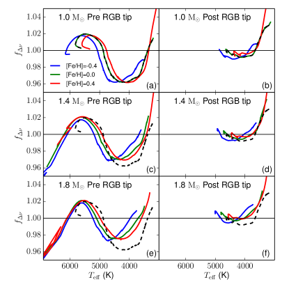
The value Hz corresponds to our adopted choice for . The stellar models show that varies with metallicity, , mass, , and age, . To estimate we ran a suite of stellar models for (corresponding to [Fe/H] ) and . For this we used the MESA (v6950) 1M_pre_ms_to_wd test suite case (Paxton et al., 2011, 2013, 2015), but without rotation or mass loss invoked. We followed the approach by White et al. (2011) to derive for each model, designed to mimic the way is measured from the data. For this we used GYRE (Townsend & Teitler, 2013) to calculate the required radial mode frequencies. An in-depth description of this model grid and some of its applications will be presented in future (Stello et al. 2016 in preparation) 555The stellar models along with a code to compute the correction factors are available at http://www.physics.usyd.edu.au/k2gap/Asfgrid.. We estimated along each stellar track ranging from the zero-age main sequence till the end of helium-core burning. The results were remeshed in a grid in space with dimensions of . The is the evolutionary state, with 0 for pre helium-ignition evolution and 1 for post helium-ignition evolution. The age, , is replaced by variables and , which are observable (Bedding et al., 2011). Then, using interpolation we computed the correction factor for each synthetic star and used it to correct . From now on we denote this derived correction factor by . We show in LABEL:teff_dnu_grid for different mass and metallicity. Red giant branch stars require a larger relative correction (left panels, K) compared to the red clump stars (right panels). For the red giant branch stars, the correction factor has a strong dependence on both temperature and metallicity (see also White et al., 2011). There is also a dependence on mass. This can be seen as a shift of the green curves in panel (c) and (e) with respect to the dashed curve, which is the equivalent from panel (a).
3. Analysis of giants
In this section we study a sample of 12964 red giants from Stello et al. (2013). The observations were obtained in Kepler’s long cadence mode (29.4 min). We first determine the selection function of the sample and then use that to select stars from a synthetic catalog generated using a stellar population synthesis model of the Milky Way. Next, we compare the properties of the observed stars with those in the synthetic catalog.
3.1. The selection function of the Kepler giants
In order to compare observations with Galactic model predictions, it is crucial that we know the selection function of the observed targets. However, so far it has not been possible to reproduce the selection function that generates the red giant sample observed by the Kepler mission. Previous attempts to characterize it can be found in Farmer et al. (2013) and Pinsonneault et al. (2014). The main source of information is the paper by Batalha et al. (2010), which describes the selection and prioritization of Kepler targets in general. The targets were classified into 13 priority groups based on their stellar parameters. The idea was to prioritize stars for which it was possible to detect exoplanets, and if possible terrestrial planets in habitable zones. The compiled list consisted of 261,636 stars, of which the top 150,000 stars were initially selected for observations. This included 5282 giants with and , but in the end 17471 stars with these and limits were observed. In other words, more than 50% of the total Kepler red giant sample came from stars that were added later on by the mission and for which the exact selection procedure is not documented. Other minor factors that complicate the selection function are as follows. Numerous additional targets were observed through the proposals by the Guest Observer program and the Kepler Asteroseismic Science Consortium. Each of these had their own complex and often undocumented selection schemes. Moreover, all stars were not observed for the same number of quarters. The length of observation puts a limit on the range of over which oscillations can be detected and characterized (e.g., Stello et al., 2015a).
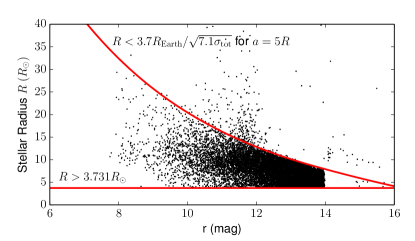
In the following, we deduce an approximate form for the selection function of the Kepler giants by comparing the properties of the observed giant sample against that of all stars in the KIC. In LABEL:sel_func_giants we plot the KIC radius against the band magnitude of stars in the KIC. The majority of stars obey a selection of the form , where is the stellar radius. The lower bound comes from the fact that the seismic analysis by Stello et al. (2013) only included stars with . In the KIC, and almost follow a one-to-one relation, hence a limit on implies a limit on . We found that was well described by (see LABEL:sel_func_giants)
| (12) |
where, is the long cadence noise given by
| (13) |
with (Jenkins et al., 2010).
The derivation of Equation 12 follows closely the scheme used by Batalha et al. (2010) to select and prioritize the planet search targets. The minimum detectable radius of a planet is given by
| (14) |
where the noise
| (15) |
depends on the number of transits, , during the lifetime of the mission, , and the number of photometric measurements per transit, , with cadence interval, . and depend on mass, , and radius, , of the host star and on the semi-major axis, , of the planet orbiting around it, as follows:
| (16) | |||
| (17) |
If the orbit radius is, say, , then for 3.5 yrs and 30 minutes we have
| (18) |
The condition that Kepler should be able to detect planets with radius greater than some predefined limit means,
| (19) |
using Equation 14. This puts the following limit on the radius of the host star
| (20) |
We found that provides a good match to the upper envelope of the stellar radius for the red giant sample (LABEL:sel_func_giants).
3.2. Comparison of photometric parameters
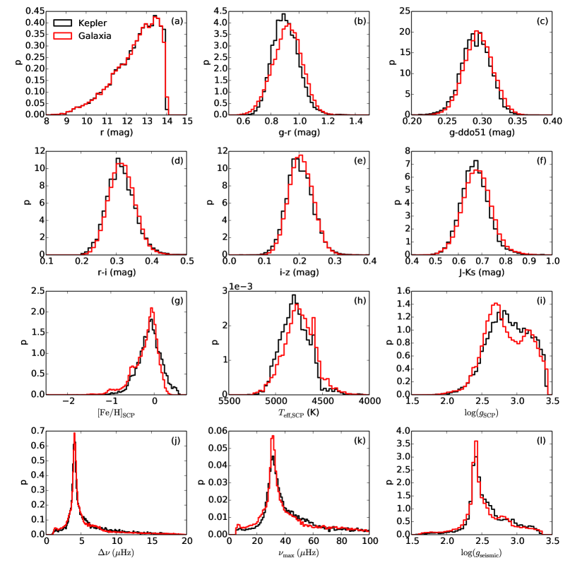
Before investigating whether the mass and radius distributions inferred from asteroseismic observations match the Galactic model predictions, we first needed to verify that we have correctly reproduced the selection function. This was done by comparing the photometric properties of the two samples. In LABEL:giants_summary we show the distributions of band magnitude, colors, SCP-derived stellar parameters, the seismic observables , , and surface gravity of our giant sample, alongside synthetic stars from the Galactic model. The seismic observables for synthetic stars were calculated using asteroseismic scaling relations (Equations 5 and 6 with ). As before, the perfect match for the band distribution (LABEL:giants_summarya) is by construction, but the good match of the color distributions (LABEL:giants_summaryb-f) and the other parameters gives confidence that the adopted selection function is correct. The SCP-derived stellar parameters also match well (LABEL:giants_summaryg-i). The slight difference in the SCP-derived gravity distribution is due to our inability to exactly reproduce SCP-derived gravity, as discussed in Section 2.2. Finally, the distribution of the seismic parameters , , and the inferred gravity also agree with the predictions of the Galactic model (LABEL:giants_summaryj-l).
3.3. Comparison of mass and radius distributions
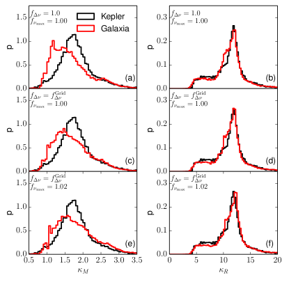
The distributions of and (Equations 9 and 10) are shown in LABEL:giants_mass. In LABEL:giants_massa,b we do not apply a correction to either of the scaling relations (), while in LABEL:giants_massc,d we set (obtained from our grid; Section 2.3). In both cases the distributions do not match. However, the use of clearly reduces the discrepancy. In LABEL:giants_masse,f, we apply a correction to the scaling relation by setting to shift to higher values improving the agreement with observations. However, the predicted distribution is still too broad (see Section 3.4 and 4 for further discussion on these issues). We also investigated if choosing higher photometric uncertainty while generating the SCP parameters had any effect on our findings (se Section 2.2). We found that choosing a higher photometric uncertainty had no significant effect on the mass and the radius distribution of the synthetic stars.
The isochrones in the Galactic model use . However, recent studies suggest a lower value of (Asplund et al., 2009; Caffau et al., 2011). To be consistent with the isochrones in the Galactic model we adopted when computing from our grid. We note that, decreasing from 0.019 to 0.012 when computing increases the predicted values of by about 6%. This increase in is similar to the increase in that occurs when is increased from 1.0 to 1.02.
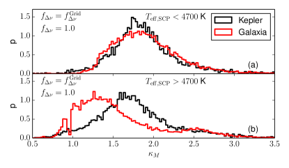
We next study if the mismatch between observed and predicted distributions has any dependence on temperature. We found that the mismatch is minimal if we restrict the sample to but becomes prominent with increasing temperature. This is shown in LABEL:kappam_teff where we plot the distributions for and . was computed with and . Also, we use SCP-based temperatures, because for observed stars we only have SCP-based temperatures. The cause behind such a temperature dependent trend is not yet clear. Firstly, these are SCP-based temperatures, which may be slightly different from the actual temperatures. The age, metallicity and temperature are correlated with each other. So, age and metallicity-based trends could also manifest themselves as temperature trends.
3.4. Kepler giants in the SAGA survey
In the previous section, we showed that the distribution of the synthetic stars generated by Galaxia does not match the observed stars. We now investigate if the mismatch is for all stars in our sample, or whether it depends on metallicity. To do this we make use of the SAGA survey, which provides metallicities for an unbiased subset of red giants observed by Kepler.
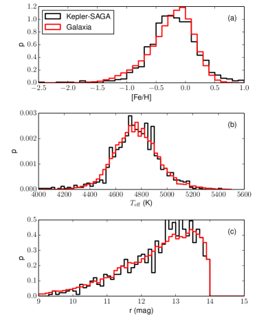
The SAGA survey (Casagrande et al., 2014) provided Strömgren photometry for giants that have seismic parameters from Kepler observations. The current release comprises, 989 Kepler red giants based on observations covering a stripe centered at galactic longitude and galactic longitude ranging . In SAGA, Strömgren photometry was combined with broadband photometry, and the infrared flux method was used to obtain with a precision of 85 K and with a precision 0.18 dex. We expect the SAGA sample to be an unbiased subset of the full Kepler red giant sample because SAGA observed almost all stars down to mag, while the seismic giants are all brighter than 14th mag in band (roughly corresponding to ). Casagrande et al. (2014) reported the SAGA giant sample to be 95% complete with respect to the seismic targets. To check for any potential bias, we compared the distribution of metallicity, temperature and band magnitude of the SAGA giants with those of the synthetic stars satisfying the Kepler red giant selection function described in Section 3.1 (LABEL:saga_comp). An uncertainty of 0.18 dex (similar to that of SAGA sample) was added to the metallicity of the synthetic stars. The good agreement between the synthetic and the observed distributions confirms that the SAGA sample is an unbiased sample of our Kepler red giant sample. No other large unbiased set of metallicities are currently available for the Kepler red giants.
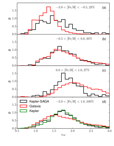
We now compare the distribution for the SAGA sample with that from the Galactic model. The values were computed using the correction factor from the grid of stellar models in Section 2.4 and assuming . LABEL:saga_mass_fcorra,b,c show that the mean increases with increasing metallicity. However, the change in is stronger in the Galactic model than in the data. The difference between the model and the data is largest for the low and the high metallicity bins, which account for 50% of the sample. For , the predictions of the Galactic model agree with observations.
LABEL:saga_mass_fcorrd shows the distribution of the SAGA sample for the full range (black) alongside the full Kepler red giant sample (green). They agree with each other, which illustrates once again that the SAGA sample is an unbiased subset of the Kepler red giant sample.
| 1 | 2 | 3 | 4 | ||||
| benchmark case | property | non-seismic | seismic | seismic | seismic | seismic | |
| NGC6791, eclipsing binary- | |||||||
| extrapolated mass. | |||||||
| Brogaard et al. (2012) | |||||||
| APOKASC metal poor giants. | (OCT) | (OCT) | (OCT) | (OCT) | |||
| Epstein et al. (2014) | (SYD) | (SYD) | (SYD) | (SYD) | |||
| KIC 8410637, a red giant | 666The predicted values are assuming the star to be a red giant branch stars, the values in square brackets are assuming the star to be a red clump star | ||||||
| in an eclipsing binary system. | |||||||
| Gaulme et al. (2013) | |||||||
| KIC 9246715, two red giants | |||||||
| in an eclipsing binary system. | |||||||
| Rawls et al. (2016) | |||||||
| HD185351, a bright giant with | |||||||
| interferometry and parallax. | |||||||
| Johnson et al. (2014) |
We note that the analysis of the SAGA sample has its limitations. The SAGA sample has a metallicity uncertainty of 0.18 dex, which is relatively large. So, the suggested range of validity of the Galactic model, , is subject to this uncertainty in metallicity. The good match of in occurs only after an ad-hoc correction of 2% to . This correction is not a prescription for a global change to the scaling relation, but is a guide to quantify the differences between model predictions and observations. We note, it is possible that different groups of stars (e.g., red clump and red giant branch), have different correction factors that negate each other. This would make such global correction factor unphysical.
4. Revisiting the asteroseismic scaling relations
Our results in the previous sections show that corrections to the scaling relations can improve the agreement between observed seismic masses and those predicted by Galaxia. The main correction was to use from the grid of stellar models. Additionally, we investigated a correction of the form , specifically for the red giants. We now compare the stellar properties like mass and radius, inferred using seismology with and without corrections to the scaling relations, against five benchmark cases where measurements are available independent of seismology. The results are summarized in Table 1 and we discuss them in detail below.
Table 1 shows that for all five benchmark cases, the standard uncorrected scaling relations, with and (option 1), overestimate the mass as compared to non-seismic estimates. We investigate different combinations of the following corrections, and (options 2-4). We see that when the correction is used, either with or 1.02 (options 3-4), the seismic estimates match the non-seismic estimates to within . Also, when using , the cluster NGC 6791 is the only benchmark case that favors (option 3) instead of (option 4). To conclude, the non seismic estimates that we study here, support the use of . Four out of five benchmark cases studied also support the use of .
| Brogaard 2011,2012 | Miglio 2012 | |
|---|---|---|
| Metallicity | 0.29 0.030.08 | |
| Distance | 13.51 0.06 | |
| Helium content | 0.3 0.01 | |
| Age | 8.3 0.40.7 | |
| 1.15 0.02 | 1.230.02 | |
| 1.150.03 |
4.1. Masses and radii of stars in the open cluster NGC 6791
Clusters provide a unique opportunity to test the scaling relations because stars in a cluster have a negligible spread in age, metallicity and distance. NGC 6791 is one of the oldest and most metal-rich open clusters known. Brogaard et al. (2012) estimated the age, the helium content, and the mass of stars on the lower red giant branch using information from two eclipsing binaries along with color magnitude diagrams of the cluster (see also Brogaard et al., 2011). The measured properties are given in Table 2.
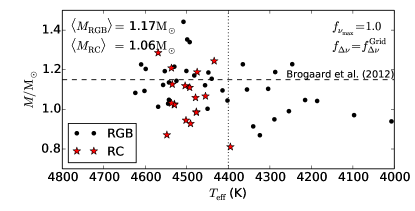
Miglio et al. (2012) used asteroseismology from Kepler data to measure the masses of the red giant branch and red clump stars in NGC6791. Their estimates of masses for the red giant branch stars were higher than found by Brogaard et al. (2012). Using photometry, temperature, and distance modulus, Miglio et al. (2012) also measured the radii of the stars independently of asteroseismology. For the red giant branch stars, they found the radius estimated from photometry to be in agreement with those estimated by asteroseismology, but for the red clump stars they found the seismic estimate to be smaller by about 5%. Miglio et al. (2012) noted that the factor suggested by their stellar models was higher for red clump stars compared to red giant branch stars. This prompted Miglio et al. (2012) to adopt for red giant branch stars and for red clump stars, which brought the seismic and non seismic estimates of radius in agreement with each other. When, using from our stellar models, we also find to be higher for red clump stars (LABEL:teff_dnu_grid). However, for NGC6791, on average the red giant branch stars have while the red clump stars have (close to unity). While the relative difference between the corrections for the two groups of stars is similar to what Miglio et al. (2012) found, our values are lower and hence our seismic estimates of radius, for both red giant branch and red clump stars, do not match the non-seismic estimates. However, a change of 0.15 mag in distance modulus, which has an uncertainty of 0.06 mag, is enough to bring the photometric and seismic estimates of radius in agreement.
Our estimates of mass, using , are shown in LABEL:ngc6791, which match well with estimates of Brogaard et al. (2012) (dashed line). When estimating the average mass of the red giant branch stars, we restricted them to be hotter than the coldest red clump star (hence less luminous than red clump stars) to avoid giants whose evolutionary state is ambiguous.
4.2. Metal poor giants in APOKASC
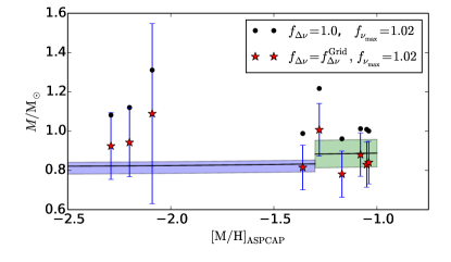
Epstein et al. (2014) studied asteroseismic masses of metal-poor stars observed by Kepler and APOGEE that were part of the APOKASC sample (Pinsonneault et al., 2014). Nine stars were found with . Seven of them were labelled as halo stars and the other two as thick disc stars, based on their kinematics. By making some assumptions on and age of these stars, Epstein et al. (2014) predicted their masses. They adopted a range of 0.2 – 0.4 for , 10 – 13.77 Gyr for the age of the halo and 8 – 13.77 Gyr for the age of the thick disc. An approximate reproduction of these predicted masses by us is shown as the shaded region in LABEL:epstein. Next, Epstein et al. (2014) measured the mean offset of seismic masses from these predictions, and found them to be . They used , which is the method-specific value for the OCT method (Hekker et al., 2010) used by them. This choice is equivalent to in our terminology (Equation 6), because we use . Our results, adopting the OCT values for the stars, with are shown in LABEL:epstein and Table 1. The results, both with and without correction, are shown (options 2 and 4). We find that adopting the correction lowers the mass on average by 0.15 and brings closer to the expected value of zero. If the OCT method really has method specific systematics then the above results do not suggest any additional correction to the scaling relation besides that required to acccount for a higher value of . For 8 out of 9 metal poor giants we also have and estimates using the SYD pipeline, for which . Results for these are also shown in Table 1. Here, option 4 is the best, this supports correction to both the and the scaling relations. A correction to the scaling relation was also suggested by Epstein et al. (2014), based on two metal poor stars, Indi (Bedding et al., 2006) and KIC 7341231 (Deheuvels et al., 2012).
4.3. Red giants in eclipsing binary systems
Detached eclipsing binaries (dEB) can be used to measure the mass and radius of each stellar component independently of asteroseismology, and hence offer the opportunity to test the asteroseismic scaling relations. Of the 13 candidate eclipsing binaries with a pulsating red giant component currently found in the Kepler data (Gaulme et al., 2013), KIC 8410637 and KIC 9246715 are the only ones that have mass and radius measured from the analysis of the eclipses in the light curves. It can be seen from Table 1 that correcting the scaling relations, with and , brings the seismic masses and radii in better agreement with the dynamical masses and radii. The correction factor , which depends upon the evolutionary state of a star, is different for a red giant branch star and a red clump star. Currently we do not have any information about the evolutionary state of these stars. In Table 1 the values corresponding to a red clump star are shown in square brackets. It can be seen that for both the stars the dynamical estimates of mass and radius favor them to be red giant branch stars rather than red clump stars.
4.4. HD185351: radius from interferometry
Long-baseline interferometry in optical/near-infrared wavelengths from instruments like CHARA (ten Brummelaar et al., 2005) allows one to measure angular diameters of stars with 1-2% accuracy (Huber et al., 2012). If distance is known, one can convert angular diameter to radius. However, accurate reliable distances, e.g., from parallax measurements, are currently only available for bright nearby stars. HD185351, with V=5.18, is the third brightest star observed by Kepler (Johnson et al., 2014) and is also nearby with a parallax-based distance of pc. By combining this distance with the interferometric measurement of the angular diameter, Johnson et al. (2014) estimated the radius to be . This estimate is slightly larger than the asteroseismic estimate of based on uncorrected scaling relations. With corrections, and , the asteroseismic estimate of radius is . which agrees better with the interferometric and parallax-based measurement.
5. Changing the Galactic model
In Section 4, we saw that the predictions of the Galaxia model do not match the mass distribution of observed red giant stars from Kepler. We investigated corrections to the asteroseismic scaling relations and found that the corrections improve the agreement with observations but do not make the disagreements go away completely. We now investigate the changes that would be required in the Galactic model to match the asteroseismic information from Kepler. The main mismatch is that the Galactic model overpredicts the number of low mass stars. The age of a red giant star is inversely related to its mass, so if we change the star-formation rate to reduce the relative fraction of old stars, the predicted mass distribution should shift towards higher masses and consequently improve the agreement.
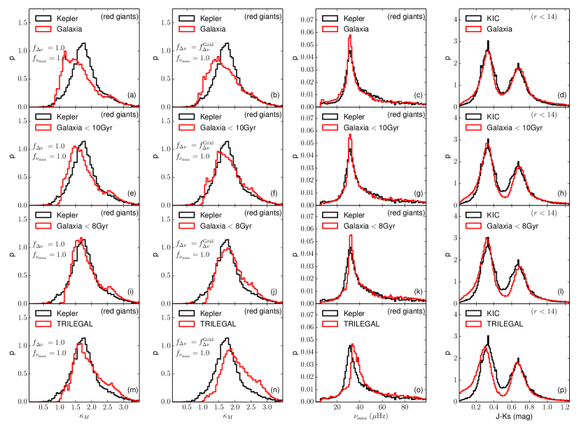
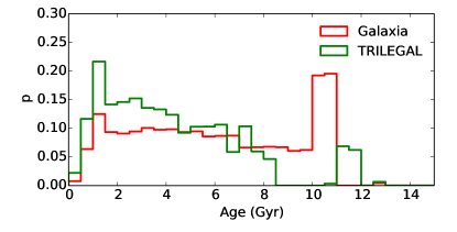
In LABEL:galaxia_trilegal_giants, each row corresponds to a different Galactic model, and for each model we plot the distribution of , , and color. The distribution of , is for the red giant sample, while the distribution is for stars in KIC with apparent magnitudes . The distributions are shown both without (first column) and with correction (second column) to the scaling relation. Panels in the top row (LABEL:galaxia_trilegal_giantsa-d) show the default Galaxia model. This has a thin disc with a constant star formation rate for age between 0 to 10 Gyr and a separate thick disc with age between 10 to 11 Gyr. In the second row (LABEL:galaxia_trilegal_giantse-h) and the third row (LABEL:galaxia_trilegal_giantsi-l) the star formation rate in Galaxia is truncated such that there are no stars older than 10 and 8 Gyr, respectively. In the bottom row (LABEL:galaxia_trilegal_giantsm-p) we use the default version of TRILEGAL, which has a two step star formation rate. Between 1 to 4 Gyr the star formation rate is 1.5 times higher than at other times (Girardi et al., 2005). We applied the same selection procedure on the TRILEGAL stars as we did for Galaxia stars, that is, band correction, estimation of stellar parameters from photometry using the SCP code, and then applying the selection function as discussed in Section 3.1. The age distributions of the red giant sample, as predicted by Galaxia and TRILEGAL, are shown in LABEL:age_dist_galaxia_trilegal_giant. The TRILEGAL model clearly has more younger stars (in the range 1 – 4 Gyr) than any Galaxia based model considered here. So, going from top row to bottom row, the percentage of young stars in the model increases. As expected, the predicted mass distributions, as shown in the first and second columns, are found to shift towards higher masses as one goes from top to bottom along each column.
We now concentrate on the top three rows in LABEL:galaxia_trilegal_giants, which are Galaxia based models, and investigate changes relative to the default Galaxia model shown in the first row (LABEL:galaxia_trilegal_giantsa-d). If we remove the very oldest stars (second row/ LABEL:galaxia_trilegal_giantse-h), the match between the Galactic model and the observations is better with the correction (panel f) than without (panel e). Hence, if the correction factor is used, only stars older than 10 Gyr, which is 19% of the Galaxia sample, need to be discarded to bring the models into reasonable agreement with the data. If we remove older stars more aggressively (third row/ LABEL:galaxia_trilegal_giantse-h) we see the opposite effect; the match is better when no correction is applied (compare panels i and j). Hence, if the correction factor is not used, stars older than 8 Gyr, which is 32% of the Galaxia sample, need to be discarded to reach a reasonable match. These results highlight the degeneracy between the star formation rate and the correction factor to the scaling relations. Since, a correction to the scaling relation also alters the mass distribution, the factor will also be degenerate with the star formation rate. The bottom row (LABEL:galaxia_trilegal_giantsm-p)) shows the TRILEGAL model, whose star formation rate is closer to the Galaxia model in third row LABEL:galaxia_trilegal_giantsi-l). Similar to that Galaxia model, the predicted mass distribution of TRILEGAL matches with observations, provided the correction factor is not used.
The models in the bottom three rows of LABEL:galaxia_trilegal_giants match the observed mass distribution better than the default Galaxia model shown in the top row (LABEL:galaxia_trilegal_giantsa,b). However, these models do not match the color distribution (fourth column), especially its blue wing where the match becomes progressively worse going from top to bottom. This is because, these models correspond to an increasingly higher fraction of young stars. The younger stars are more blue (hotter) giving rise to an increased number of stars in the blue wing of the color distribution. In addition to the mismatch with the observed color distribution, the TRILEGAL model, also shows a mismatch with the observed distribution. Note that the corrections in 2.1.1 have no effect on the distributions shown here. This is because any potential inaccuracies in photometry are related to Kepler and bands and not the 2MASS and bands. Also, issues related to the red giant selection function, as discussed in 2.2 and 3.1, also have no effect on the distributions shown here, because the color distribution is shown for a simple magnitude limited sample satisfying .
The star formation rate is not the only part of the model that can alter the mass distribution. Changing the age scale height and age scale radius relation in the Galactic model will alter the age distribution and thereby the mass distribution of stars selected with the Kepler selection function. Changing the initial mass function of stars in the Galactic model can also alter the mass distribution. Clearly, in future, when attempting to fit a Galactic model to observed data, one should take all of the above mentioned factors into account.
6. Summary and Conclusions
In this paper, we explored the prospect of using asteroseismic information of red giants to constrain stellar population synthesis-based models of the Milky Way. We used a sample of about 13,000 red giants from the Kepler mission. The large sample size allowed us to test the Galactic models with asteroseismic data at a level that was not possible before. For the first time, within the framework of stellar population synthesis-based modelling, we also investigated changes to the Galactic model and the asteroseismic relations.
The asteroseismic scaling relations provide a practical way to determine mass and radius from average asteroseismic parameters like and for a large number of stars. However, the range of validity of these relations is not yet clear, specially for red giants whose structure is not homologous to that of the Sun. In previous studies it has been shown that estimated from theoretically calculated oscillation frequencies differs from the simple scaling with density. To investigate this, we estimated corrections to the scaling relation as a function of mass, metallicity, temperature and evolutionary state, using a grid of stellar models. We found that the Galactic model that best matched the photometry fitted the asteroseismic data better if the corrections were implemented. We also studied five benchmark cases, where non-seismic estimates of mass are available, and for all of them the use of the correction brought seismic estimates closer to non-seismic estimates. This provides additional support for the correction.
Analysis of the SAGA sample, which provides metallicity for an unbiased subsample of Kepler giants, allowed us to explore how the agreement between the Galactic predictions and observed seismic information depends on metallicity. We find that the best match of the Galaxia model with observations is in the range . However, in addition to correction to the scaling relation, a 2% correction to the scaling relation is also required. The correction factor serves to quantify the difference between theory and observations and should not be used as a prescription for changing the seismic scaling relation. The correction is based purely on comparing the distribution of masses, and it is possible that red giant branch and red clump stars have opposite corrections that cancel each other.
Even after using the correction to the scaling relation, the Galactic model of Galaxia that best matches the photometric information fails to match the seismic information for giants. The mismatch is minimal for but is significant for . In general, Galaxia tends to overestimate the number of low mass stars, which implies that Galaxia overpredicts the number of old stars. Further corrections to asteroseismic scaling relations is certainly a possibility to resolve the discrepancy, as is a modification to the Galactic model. If the scaling relations along with corrections suggested by stellar models are correct, then at least 20% of the oldest stars in Galaxia have to be discarded to bring the predicted mass distributions in agreement with observations. However, altering the star formation rate as suggested above makes the color distributions disagree with observations. There are other model parameters that we have not yet explored, which can also alter the mass distribution of stars, such as, the age-scale height relation, age scale radius relation and the initial mass function. It is possible that some combination of these can explain both the photometric information of stars as well as the asteroseismic information. This should be explored in future. Also, to resolve degeneracies between parameters governing the model, one would need to explore observational data from multiple sources, like, asteroseismic, photometric, spectroscopic and astrometric missions.
Other than Galaxia, we also compared the predictions of the TRILEGAL Galactic model with the Kepler data. While Galaxia matches the photometry of stars in the KIC, TRILEGAL could not; it overestimated the number of blue stars. The peak in the distribution for TRILEGAL was also shifted compared to the Kepler observations. Suppressing older stars in Galaxia, also leads to overestimation of blue stars as seen in TRILEGAL. This suggests that TRILEGAL overestimates the occurrence of younger stars. However, TRILEGAL matches the mass distribution of Kepler red giants, provided no corrections are applied to .
Although we have been able to derive a selection function for the Kepler red giant sample that seems to be representative of the population, we caution that it might have some inaccuracies given the complex selection procedure involved in the actual selection of targets. Hence, it is important to verify the current findings using an independent sample of stars obeying an unambiguous selection function, such as, the red giants observed by K2 for galactic archaeology purposes, where stars have been targeted with a well defined color magnitude limits (Stello et al., 2015b).
To conclude, our results clearly demonstrate that the size and quality of asteroseismic data provided by Kepler can, in principle, provide good constraints on Galactic model parameters. However, further work is required to validate the accuracy of asteroseismic scaling relation-based mass estimates for giants and to explore a wider variety of changes to the Galactic model input. Missions like K2, TESS, and PLATO are going to increase the seismic sample size by two orders of magnitude. There are also plans to get high resolution spectroscopic data for many of these stars, which will help to explore the connection between age and chemistry. Such data, when combined with distances from Gaia, will be invaluable for modelling the Milky Way and trying to understand its formation.
Acknowledgments
We acknowledge the support of Galactic Archaeology and Precision Stellar Astrophysics program organized by Kavli Institute for Theoretical Physics (National Science Foundation Grant No. NSF PHY11-25915) for facilitating helpful discussions of results in this paper; especially Mark Pinsonneault, Andrea Miglio, Victor Silva Aguirre and Aldo Serenelli. SS is funded through Australian Research Council (ARC) DP grant 120104562 (PI Bland-Hawthorn) which supports the HERMES project. JBH is funded through Laureate Fellowship from the ARC. D.H. acknowledges support by the ARC’s DP grant DE140101364 and support by the NASA under Grant NNX14AB92G issued through the Kepler Participating Scientist Program.
References
- Asplund et al. (2009) Asplund, M., Grevesse, N., Sauval, A. J., & Scott, P. 2009, ARA&A, 47, 481
- Balmforth (1992) Balmforth, N. J. 1992, MNRAS, 255, 603
- Batalha et al. (2010) Batalha, N. M., Borucki, W. J., Koch, D. G., et al. 2010, ApJ, 713, L109
- Bedding (2014) Bedding, T. R. 2014, Solar-like oscillations: An observational perspective (Pallé, P. L. and Esteban, C.), 60
- Bedding et al. (2006) Bedding, T. R., Butler, R. P., Carrier, F., et al. 2006, ApJ, 647, 558
- Bedding et al. (2011) Bedding, T. R., Mosser, B., Huber, D., et al. 2011, Nature, 471, 608
- Belkacem (2012) Belkacem, K. 2012, in SF2A-2012: Proceedings of the Annual meeting of the French Society of Astronomy and Astrophysics, ed. S. Boissier, P. de Laverny, N. Nardetto, R. Samadi, D. Valls-Gabaud, & H. Wozniak, 173–188
- Belkacem et al. (2011) Belkacem, K., Goupil, M. J., Dupret, M. A., et al. 2011, A&A, 530, A142
- Belkacem et al. (2013) Belkacem, K., Samadi, R., Mosser, B., Goupil, M.-J., & Ludwig, H.-G. 2013, in Astronomical Society of the Pacific Conference Series, Vol. 479, Progress in Physics of the Sun and Stars: A New Era in Helio- and Asteroseismology, ed. H. Shibahashi & A. E. Lynas-Gray, 61
- Bertelli et al. (1994) Bertelli, G., Bressan, A., Chiosi, C., Fagotto, F., & Nasi, E. 1994, A&AS, 106, 275
- Brogaard et al. (2011) Brogaard, K., Bruntt, H., Grundahl, F., et al. 2011, A&A, 525, A2
- Brogaard et al. (2012) Brogaard, K., VandenBerg, D. A., Bruntt, H., et al. 2012, A&A, 543, A106
- Brown et al. (1991) Brown, T. M., Gilliland, R. L., Noyes, R. W., & Ramsey, L. W. 1991, ApJ, 368, 599
- Brown et al. (2011) Brown, T. M., Latham, D. W., Everett, M. E., & Esquerdo, G. A. 2011, AJ, 142, 112
- Bruntt et al. (2010) Bruntt, H., Bedding, T. R., Quirion, P.-O., et al. 2010, MNRAS, 405, 1907
- Caffau et al. (2011) Caffau, E., Ludwig, H.-G., Steffen, M., Freytag, B., & Bonifacio, P. 2011, Sol. Phys., 268, 255
- Casagrande et al. (2014) Casagrande, L., Silva Aguirre, V., Stello, D., et al. 2014, ApJ, 787, 110
- Chaplin et al. (2008) Chaplin, W. J., Houdek, G., Appourchaux, T., et al. 2008, A&A, 485, 813
- Chaplin & Miglio (2013) Chaplin, W. J., & Miglio, A. 2013, ARA&A, 51, 353
- Chaplin et al. (2011) Chaplin, W. J., Kjeldsen, H., Christensen-Dalsgaard, J., et al. 2011, Science, 332, 213
- Coelho et al. (2015) Coelho, H. R., Chaplin, W. J., Basu, S., et al. 2015, MNRAS, 451, 3011
- Deheuvels et al. (2012) Deheuvels, S., García, R. A., Chaplin, W. J., et al. 2012, ApJ, 756, 19
- Epstein et al. (2014) Epstein, C. R., Elsworth, Y. P., Johnson, J. A., et al. 2014, ApJ, 785, L28
- ESA (1997) ESA, ed. 1997, ESA Special Publication, Vol. 1200, The HIPPARCOS and TYCHO catalogues. Astrometric and photometric star catalogues derived from the ESA HIPPARCOS Space Astrometry Mission
- Farmer et al. (2013) Farmer, R., Kolb, U., & Norton, A. J. 2013, MNRAS, 433, 1133
- Frandsen et al. (2013) Frandsen, S., Lehmann, H., Hekker, S., et al. 2013, A&A, 556, A138
- Gaulme et al. (2013) Gaulme, P., McKeever, J., Rawls, M. L., et al. 2013, ApJ, 767, 82
- Girardi et al. (2005) Girardi, L., Groenewegen, M. A. T., Hatziminaoglou, E., & da Costa, L. 2005, A&A, 436, 895
- Hekker et al. (2013) Hekker, S., Elsworth, Y., Mosser, B., et al. 2013, A&A, 556, A59
- Hekker et al. (2010) Hekker, S., Broomhall, A.-M., Chaplin, W. J., et al. 2010, MNRAS, 402, 2049
- Hekker et al. (2011) Hekker, S., Gilliland, R. L., Elsworth, Y., et al. 2011, MNRAS, 414, 2594
- Houdek et al. (1999) Houdek, G., Balmforth, N. J., Christensen-Dalsgaard, J., & Gough, D. O. 1999, A&A, 351, 582
- Huber et al. (2009) Huber, D., Stello, D., Bedding, T. R., et al. 2009, Communications in Asteroseismology, 160, 74
- Huber et al. (2011) Huber, D., Bedding, T. R., Stello, D., et al. 2011, ApJ, 743, 143
- Huber et al. (2012) Huber, D., Ireland, M. J., Bedding, T. R., et al. 2012, ApJ, 760, 32
- Huber et al. (2013) Huber, D., Chaplin, W. J., Christensen-Dalsgaard, J., et al. 2013, ApJ, 767, 127
- Jenkins et al. (2010) Jenkins, J. M., Caldwell, D. A., Chandrasekaran, H., et al. 2010, ApJ, 713, L120
- Johnson et al. (2014) Johnson, J. A., Huber, D., Boyajian, T., et al. 2014, ApJ, 794, 15
- Kjeldsen & Bedding (1995) Kjeldsen, H., & Bedding, T. R. 1995, A&A, 293, 87
- Marigo et al. (2008) Marigo, P., Girardi, L., Bressan, A., et al. 2008, A&A, 482, 883
- Miglio et al. (2009) Miglio, A., Montalbán, J., Baudin, F., et al. 2009, A&A, 503, L21
- Miglio et al. (2012) Miglio, A., Brogaard, K., Stello, D., et al. 2012, MNRAS, 419, 2077
- Miglio et al. (2013a) Miglio, A., Chiappini, C., Morel, T., et al. 2013a, in European Physical Journal Web of Conferences, Vol. 43, European Physical Journal Web of Conferences, 3004
- Miglio et al. (2013b) Miglio, A., Chiappini, C., Morel, T., et al. 2013b, MNRAS, 429, 423
- Mosser et al. (2010) Mosser, B., Belkacem, K., Goupil, M.-J., et al. 2010, A&A, 517, A22
- Mosser et al. (2013) Mosser, B., Michel, E., Belkacem, K., et al. 2013, A&A, 550, A126
- Paxton et al. (2011) Paxton, B., Bildsten, L., Dotter, A., et al. 2011, ApJS, 192, 3
- Paxton et al. (2013) Paxton, B., Cantiello, M., Arras, P., et al. 2013, ApJS, 208, 4
- Paxton et al. (2015) Paxton, B., Marchant, P., Schwab, J., et al. 2015, ApJS, 220, 15
- Perryman (2002) Perryman, M. A. C. 2002, Ap&SS, 280, 1
- Pinsonneault et al. (2012) Pinsonneault, M. H., An, D., Molenda-Żakowicz, J., et al. 2012, ApJS, 199, 30
- Pinsonneault et al. (2014) Pinsonneault, M. H., Elsworth, Y., Epstein, C., et al. 2014, ApJS, 215, 19
- Rawls et al. (2016) Rawls, M. L., Gaulme, P., McKeever, J., et al. 2016, ArXiv e-prints, arXiv:1601.00038
- Robin & Creze (1986) Robin, A., & Creze, M. 1986, A&A, 157, 71
- Robin et al. (2003) Robin, A. C., Reylé, C., Derrière, S., & Picaud, S. 2003, A&A, 409, 523
- Sandquist et al. (2013) Sandquist, E. L., Mathieu, R. D., Brogaard, K., et al. 2013, ApJ, 762, 58
- Sharma et al. (2011) Sharma, S., Bland-Hawthorn, J., Johnston, K. V., & Binney, J. 2011, ApJ, 730, 3
- Sharma et al. (2014) Sharma, S., Bland-Hawthorn, J., Binney, J., et al. 2014, ApJ, 793, 51
- Silva Aguirre et al. (2012) Silva Aguirre, V., Casagrande, L., Basu, S., et al. 2012, ApJ, 757, 99
- Stello et al. (2009) Stello, D., Chaplin, W. J., Basu, S., Elsworth, Y., & Bedding, T. R. 2009, MNRAS, 400, L80
- Stello et al. (2013) Stello, D., Huber, D., Bedding, T. R., et al. 2013, ApJ, 765, L41
- Stello et al. (2015a) Stello, D., Huber, D., Sharma, S., et al. 2015a, ArXiv e-prints, arXiv:1506.08931
- Stello et al. (2015b) —. 2015b, ApJ, 809, L3
- ten Brummelaar et al. (2005) ten Brummelaar, T. A., McAlister, H. A., Ridgway, S. T., et al. 2005, ApJ, 628, 453
- Townsend & Teitler (2013) Townsend, R. H. D., & Teitler, S. A. 2013, MNRAS, 435, 3406
- Ulrich (1986) Ulrich, R. K. 1986, ApJ, 306, L37
- Verner et al. (2011) Verner, G. A., Chaplin, W. J., Basu, S., et al. 2011, ApJ, 738, L28
- White et al. (2011) White, T. R., Bedding, T. R., Stello, D., et al. 2011, ApJ, 743, 161