Multiple radial positive solutions of semilinear elliptic problems with Neumann boundary conditions

Abstract.

Assuming $B_{R}$ is a ball in $\mathbb{R}^{N}$, we analyze the positive solutions of the problem

$$\left\{\begin{aligned} -\Delta u+u&=\mathopen{|}u\mathclose{|}^{p-2}u,&&\text{ in }B_{R},\\ \partial_{\nu}u&=0,&&\text{ on }\partial B_{R},\end{aligned}\right.$$

that branch out from the constant solution $u=1$ as $p$ grows from $2$ to $+\infty$. The non-zero constant positive solution is the unique positive solution for $p$ close to $2$. We show that there exist arbitrarily many positive solutions as $p\to\infty$ (in particular, for supercritical exponents) or as $R\to\infty$ for any fixed value of $p>2$, answering partially a conjecture in [12]. We give the explicit lower bounds for $p$ and $R$ so that a given number of solutions exist. The geometrical properties of those solutions are studied and illustrated numerically. Our simulations motivate additional conjectures. The structure of the least energy solutions (among all or only among radial solutions) and other related problems are also discussed.

1. Introduction

In this paper, we consider the semilinear elliptic problem

$$\left\{\begin{aligned} -\Delta u+\lambda u&=\mathopen{|}u\mathclose{|}^{p-2}u,&&\text{ in }\Omega,\\ u&>0,&&\text{ in }\Omega,\\ \partial_{\nu}u&=0,&&\text{ on }\partial\Omega,\end{aligned}\right. \mathcal{P}_{\lambda,p}$$ ()

where $\Omega$ is a smooth bounded domain in $\mathbb{R}^{N}$, $N\geqslant 3$, $\lambda>0$, $p>2$ and $\partial_{\nu}$ denotes the outward normal derivative. This problem, sometimes referred to as the Lane-Emden equation with Neumann boundary conditions, arises for instance in mathematical models which aim to study pattern formation, and more specifically in those governed by diffusion and cross-diffusion systems [50]. The problem is also related to the stationary Keller-Segel system in chemotaxis [35, 30, 34, 39].

As ($\mathcal{P}_{\lambda,p}$) admits a constant solution, the solvability of ($\mathcal{P}_{\lambda,p}$) differs from the case of positive solutions of the Lane-Emden equation with Dirichlet boundary conditions

$$\left\{\begin{aligned} -\Delta u&=\mathopen{|}u\mathclose{|}^{p-2}u,&&\text{ in }\Omega,\\ u&>0,&&\text{ in }\Omega,\\ u&=0,&&\text{ on }\partial\Omega,\end{aligned}\right.$$ (1.1)

for which it is well known that, if $\Omega$ is starshaped and $N\geqslant 3$, existence is restricted to the subcritical range

$$p<2^{*}:=\frac{2N}{N-2}$$ (1.2)

as a consequence of Pohozaev’s identity (see [56]). In the sequel of the paper we set $2^{*}=+\infty$ if $N=2$.

The subcriticality assumption (1.2) allows to tackle the problem ($\mathcal{P}_{\lambda,p}$) with variational methods, i.e., the equation arises as the Euler-Lagrange equation of the energy functional

$$\mathcal{E}_{\lambda,p}:H^{1}(\Omega)\to\mathbb{R}:u\mapsto\frac{1}{2}\int_{\Omega}\mathopen{|}\nabla u\mathclose{|}^{2}+\lambda u^{2}-\frac{1}{p}\int_{\Omega}\mathopen{|}u\mathclose{|}^{p}.$$

Moreover, due to the compact embedding $H^{1}(\Omega)\hookrightarrow L^{p}(\Omega)$, the existence of a solution to ($\mathcal{P}_{\lambda,p}$) follows by standard arguments. Indeed, it is enough to minimize ${{\mathcal{E}}}_{\lambda,p}$ on the Nehari manifold

$$\mathcal{N}_{\lambda,p}:=\bigl{\{}u\in H^{1}\setminus\{0\}:{{\mathcal{E}}}_{\lambda,p}^{\prime}(u)[u]=0\bigr{\}}$$

and to observe that the minimizer is nonnegative whereas the strong maximum principle implies its positivity. The minimizers are called least energy or ground state solutions. Looking at the quadratic form ${{\mathcal{E}}}_{\lambda,p}^{\prime\prime}(u_{0})[u,u]$, it is easily seen that any minimizer $u_{0}$ is non constant if $\lambda(p-2)>\lambda_{2}(\Omega)$. On the other hand, if $\lambda$ is small, the only minimizer is the constant solution as Lin, Ni and Takagi [39] proved that uniqueness holds for ($\mathcal{P}_{\lambda,p}$) for $\lambda$ small.

In contrast with the nonexistence result for (1.1), the energy functional for the critical exponent, ${{\mathcal{E}}}_{\lambda,2^{*}}$, achieves its minimum on ${{\mathcal{N}}}_{\lambda,2^{*}}$. Moreover, Wang [65] proved that when $\lambda$ is sufficiently large, the constant solution cannot be a minimizer.

For $\lambda$ small and $p=2^{*}$, Lin and Ni [38] conjectured that the constant solution must be the unique solution. The conjecture was studied by Adimurthi and Yadava [2, 3] and Budd, Knapp and Peletier [17] in the case of radial solutions when $\Omega$ is a ball. It happens that in this case, the conjecture is true in dimension $N=3$ or $N\geqslant 7$, while it is false in dimension $N=4,5,6$. The conjecture was further extended to convex domains in dimension $N=3$ and has lead to many developments in the recent years. We refer to [64] and to the references therein for further details.

In the supercritical range, namely when $p>2^{*}$, most of the previous works on the existence of solutions of ($\mathcal{P}_{\lambda,p}$) are devoted to perturbative cases where either $\lambda\to+\infty$ or a slightly supercritical exponent $2^{*}+\varepsilon$ is considered, see e.g. [25, 60, 61]. By scaling, it is easily seen that the case $\lambda\to+\infty$ amounts to consider a small diffusion coefficient $\varepsilon$ (in front of $-\Delta$), see below. In this setting, it is physically relevant to study the existence of solutions which concentrates around a single or multiple points or even around some curve or a higher dimensional manifold as $\varepsilon\to 0$, see for example [1, Chapter 9 and 10], [53, 54, 5, 44, 24, 42, 43, 45] and the references therein.

In this paper, we deal with ($\mathcal{P}_{\lambda,p}$) in a “non-perturbative way” and therefore our contribution is more closely related to the recent works [8, 13, 31, 62, 12]. It was observed in [62] that when $\Omega=B_{R}$ is a ball of radius $R>0$, compactness can be recovered in the supercritical case by considering the subspace of radially increasing functions of $H^{1}_{\text{rad}}(B_{R})$, where $H^{1}_{\text{rad}}(B_{R})$ is the space of functions of $H^{1}(B_{R})$ invariant under the action of the group $O(N)$. This fact was used in [12] to prove the existence of a non-constant radially increasing solution of ($\mathcal{P}_{\lambda,p}$) in the supercritical regime, i.e., without assuming (1.2), under the assumption that

$$\lambda(p-2)>\lambda^{\text{rad}}_{2}(B_{R}).$$

In the critical case, the existence of such a radially increasing solution has been proved using a shooting argument and the Emden-Fowler transformation in [2] under the same assumption

$$\lambda(2^{*}-2)>\lambda^{\text{rad}}_{2}(B_{R}).$$

This condition is satisfied if $R$ is large enough.

In our study of ($\mathcal{P}_{\lambda,p}$), one of our main motivation is to understand to what extent the precise value of $p$ plays a role in the existence and qualitative properties of solutions. Our main results are multiplicity of solutions with respect to the value of the power $p$, without assuming subcriticality. It has been shown in [12, 31, 62] that for the Neumann problem ($\mathcal{P}_{\lambda,p}$) in a ball, no growth restriction is needed to prove the existence of at least one non constant solution. Since we deal with a simpler model than in the quoted references, we are able to perform here a refined analysis. Namely, we obtain non trivial solutions that branch out from the constant solution, see Section 3. Combined with a priori estimates, this leads to the following multiplicity result.

Theorem 1.1.

Assume $\Omega=B_{R}$ , $N\geqslant 2$, $n\in\mathbb{N}_{0}$, $p\in\mathopen{]}2,+\infty\mathclose{[}$ and $\lambda>0$.

1. If $\lambda(p-2)>\lambda^{\text{rad}}_{n+1}(B_{R})$, then Problem ($\mathcal{P}_{\lambda,p}$) has at least $n$ distinct non constant radial solutions.

2. If $\lambda(p-2)>\lambda^{\text{rad}}_{n+1}(B_{R})$ and $p<2^{*}$, then ($\mathcal{P}_{\lambda,p}$) possesses at least $2n$ distinct non constant radial solutions.

3. If $\lambda(2^{*}-2)>\lambda^{\text{rad}}_{n+1}(B_{R})$ and $N\geqslant 3$, there exists $\varepsilon_{n,R}>0$ such that if

   $$\lambda^{\text{rad}}_{n+1}(B_{R})-\varepsilon_{n,R}<\lambda(p-2)<\lambda^{\text{rad}}_{n+1}(B_{R}),$$

   then ($\mathcal{P}_{\lambda,p}$) has at least $2n$ distinct non constant radial solutions.

This theorem implies the existence of arbitrarily many solutions for either large $p$ or large $R$. We anticipate that the $n$ solutions $u_{i}$ are distinguished by the number of nodal regions of $u_{i}-1$ (and also by the number of critical points). Indeed, the bifurcation analysis shows that, given a positive integer $n$, ($\mathcal{P}_{\lambda,p}$) has at least one radial solution $u$ such that $u-1$ has $n$ nodal regions provided $p>2+\lambda^{\text{rad}}_{n+1}(B_{R})/\lambda$ (see Section 3 for more details). We also anticipate that the validity of (iii) relies on a key estimate of Bessel’s function (see Lemma 3.2). Numerical evidence shows it to be valid in dimension $N=2$ but this is not formally proved.

Figure 1. Radial bifurcation branches from $2+\lambda^{\text{rad}}_{i}/\lambda$, $i=2,3$ when $2+\lambda^{\text{rad}}_{1}/\lambda<2+\lambda^{\text{rad}}_{2}/\lambda<2^{*}$.

Theorem 1.1 contrasts with the classical uniqueness result [28] of either radial or non radial solutions of (1.1) in a ball. Even in the case of an annulus where uniqueness may fail — coexistence of radial and non radial solutions was first observed in [14] — uniqueness in the class of radial solutions was proved in [51]. Multiplicity for ($\mathcal{P}_{\lambda,p}$) was observed in [13] where the existence of at least three non constant solutions is proved but the results therein are perturbative, assuming $p\to\infty$, and only concern the case of an annulus.

Theorem 1.1 is consistent with the analysis of [65] in the critical case $p=2^{*}$. One of the added value of our result is that it holds for any $p>2$ and gives further and precise informations on the multiplicity of solutions and not solely on the existence.

The structure of the bifurcations (see Fig. 1) also allows to identify degenerate radial solutions along some of the branches (see Theorem 3.12). This leads to another striking difference between the problems ($\mathcal{P}_{\lambda,p}$) and (1.1) as it is known that the positive solution to (1.1) is non-degenerate when $\Omega$ is a ball [21, 59, 36] or a “large” annulus [7].

The bifurcation analysis can also be performed without assuming radial symmetry of the domain $\Omega$, see also [52]. However, in this case, it seems necessary to restrict ourselves to a nonlinearity with subcritical growth. Also we do not have such a precise picture of the bifurcations since non simple eigenvalues may arise and the study of the behavior of solutions along a branch is much more delicate. In particular, we cannot expect any a priori bounds in the supercritical regime and we expect bifurcations from infinity.

Even in the case of a radially symmetric domain, non-radial bifurcations appear, for instance at the first bifurcation point. Indeed, this first bifurcation occurs at a non-radial eigenvalue of the elliptic operator (see Section 3). Nevertheless, the corresponding eigenfunctions are axially symmetric. As we can perform our bifurcation analysis in the space of axially symmetric functions and since it provides axially symmetric functions along the branches, it is natural to conjecture that the first bifurcation is responsible of the symmetry breaking of the least energy solution when $2+\lambda_{2}(B_{R})/\lambda<2^{*}$ (as it is also expected that $u=\lambda^{1/(p-2)}$ is the unique positive least energy solution for $p\leqslant 2+\lambda_{2}(B_{R})/\lambda$). Moreover, we conjecture that this first bifurcation is unbounded in $p$ leading to the existence of a non-radial solution for large $p$ on large balls or for large $\lambda$ (see Section 6.1).

Conjecture 1.2.

Let $N\geqslant 3$, $\lambda>0$, $\Omega=B_{R}$ and $2+\lambda_{2}(B_{R})/\lambda<2^{*}$. For every $p\in\mathopen{]}2+\lambda_{2}(B_{R})/\lambda,\,+\infty\mathclose{[}$, there exists a positive non radial solution of ($\mathcal{P}_{\lambda,p}$) which is axially symmetric.

Concerning the qualitative properties of the least energy solutions to Problem ($\mathcal{P}_{\lambda,p}$), Lopes showed that such a solution is even with respect to a family of hyperplanes, see [40], and in fact it is furthermore cap symmetric, see [66]. Moreover, Lopes showed that either the least energy solution is constant or it is non-radially symmetric. We provide in Section 5 an alternative and shorter proof of this fact. This in turn provides the upper bound $2+\lambda_{2}(B_{R})/\lambda$ on the exponent $p$ at which the radial symmetry of least energy solutions is lost. For $p$ close to $2$, as a consequence of [11], any least energy solution of ($\mathcal{P}_{\lambda,p}$) is invariant under the action of the symmetry group of the domain $\Omega$. For instance, in radial domains, these are radial functions. According to the previous discussion, this suggests, at least for the ball, that for $p$ close to $2$, any least energy solution is in fact constant. This is actually true for every domain, see Theorem 2.3. Numerical experiments, based on the mountain pass algorithm, suggest that $2+\lambda_{2}(B_{R})/\lambda$ is the exact threshold for the existence of non constant least energy solutions, see Section 6.

Conjecture 1.3.

Let $N\geqslant 2$, $\lambda>0$, $p\in\mathopen{]}2,2^{*}\mathclose{[}$ and $\Omega=B_{R}$. The positive constant solution is the least energy solution to ($\mathcal{P}_{\lambda,p}$) if and only if $p<2+\lambda_{2}(B_{R})/\lambda$ and there is no other positive solution in this range of the parameters. For $p>2+\lambda_{2}(B_{R})/\lambda$, the least energy solutions are not radially symmetric and belong to the branch bifurcating from $(p,u)=\bigl{(}2+\lambda_{2}(B_{R})/\lambda,\lambda^{1/(p-2)}\bigr{)}$.

Our numerical simulations also complements the papers [53, 54] where it was shown that, on a smooth domain $\Omega$, the least energy solutions $u_{\varepsilon}$ of

$$\left\{\begin{aligned} -{\varepsilon}\,\Delta u+u&=f(u),&&\text{ in }B_{R},\\ u&>0,&&\text{ in }B_{R},\\ \partial_{\nu}u&=0,&&\text{ on }\partial B_{R}\end{aligned}\right. \mathcal{P}_{\varepsilon}$$ ()

with $f(u)=\mathopen{|}u\mathclose{|}^{p-2}u$ with $2<p<2^{*}$ concentrate, as $\varepsilon\to 0$, around a single point of the boundary $\partial\Omega$. If $\Omega=B_{R}$, this obviously means that when $R$ is large, the radial symmetry of least energy solutions breaks down at any fixed subcritical exponent. Our analytical results and the numerical simulations indicate that “large” likely means $1+\lambda_{2}(B_{R})<2^{*}$.

In Section 4, we apply our radial bifurcation analysis on the problem ($\mathcal{P}_{\varepsilon}$). The parameter $\varepsilon>0$ aims here to model a small diffusion. By a simple scaling argument, it is easily seen that Problem ($\mathcal{P}_{\varepsilon}$) with $f(u)=\mathopen{|}u\mathclose{|}^{p-2}u$ is equivalent to ($\mathcal{P}_{\lambda,p}$) with $\lambda=1$ in the ball $B_{R/\sqrt{\varepsilon}}$. We require few assumptions on $f$. Namely, $f$ is of class $\mathcal{C}^{1}$ and satisfies, for some $u_{0}>0$,

$$f(0)=f^{\prime}(0)=0; F_{0}$$ ()

$$f(u_{0})=u_{0}\quad\text{and}\quad f^{\prime}(u_{0})>1; F_{1}$$ ()

$$F(s)-\frac{s^{2}}{2}<\varliminf_{s\to+\infty}\left(F(s)-\frac{s^{2}}{2}\right)\text{ for }0\leqslant s\leqslant u_{0},\ F_{2}$$ ()

where $F(s):=\int_{0}^{s}f(t)\,{\mathrm{d}}t$. Assumption ($F_{1}$) implies in particular that $u_{0}$ is a solution. The third assumption provides a priori bounds for a large family of solutions which bifurcate from the constant solution $u_{0}$.

Theorem 1.4.

Assume $f\in\mathcal{C}^{1}$ satisfies ($F_{0}$), ($F_{1}$), ($F_{2}$), and $N\geqslant 2$. Then for any $n\in\mathbb{N}_{0}$ and any $\varepsilon>0$ such that $\varepsilon<({f^{\prime}(u_{0})-1})/{\lambda^{\text{rad}}_{n+1}(B_{R})}$, Problem ($\mathcal{P}_{\varepsilon}$) has at least $n$ distinct non-constant radial solutions.

If we assume further that $f$ has a subcritical growth, then we can prove the existence of more solutions, at least $2n$ actually, as in the case of a pure power. Theorem 1.4 should be compared with [52]. Since we deal with a radially symmetric domain, we are able to go much deeper into the bifurcation analysis. Except from the restrictive assumption on the domain, our assumptions on the nonlinearity $f$ are quite general. In particular, $f$ can have a fast growth at infinity. Notice also that Theorem 1.4 is not of perturbative nature since we precisely characterize the values of $\varepsilon$ at which new solutions arise. The conclusion of Theorem 1.4 can be made more precise when $f(s)=s^{p}$, see [48, Theorem B] which will be discussed in Section 4.

We also emphasize that our solutions do not display interior concentrations as $\varepsilon\to 0$ in opposition to e.g. [22, 32]. Actually, our families of solutions correspond to boundary clustered layer solutions, that is solutions with many local maxima accumulating on the boundary when $\varepsilon\to 0$. In particular, the bifurcation analysis provides an easy approach to find the boundary clustered layer solutions of [5, Corollary 1.3] and [44, Theorem 1.1]. In fact, the bifurcation analysis gives the complete picture of radial clustering solutions completing those obtained in [5, 44]. For results in that direction in a non symmetric setting, we refer to [24, 42, 43, 45].

The paper is organized as follows. Section 2 deals with a priori bounds, both with or without assuming radial symmetry, which are crucial in the bifurcation analysis of ($\mathcal{P}_{\lambda,p}$). In Section 3, we first give a general insight on the bifurcation analysis and then a refined analysis of the radial bifurcations when $\Omega$ is a ball leads to Theorem 1.1. In Section 4, we prove Theorem 1.4. Section 5 deals with the qualitative properties of the least energy solutions in a ball. Finally, Section 6 contains numerical simulations and further conjectures.

2. A priori estimates

In this Section, we derive a priori estimates on positive solutions. These are helpful to control the norm of the solution along the branches bifurcating from the constant solution. Of course, the dependence on the bifurcation parameter is important and will be emphasized. We start with a uniform $L^{1}$ bound.

Lemma 2.1.

Any nonnegative solution $u$ of ($\mathcal{P}_{\lambda,p}$) satisfies

$$\int_{\Omega}u^{p-1}=\lambda\int_{\Omega}u\leqslant\lambda^{(p-1)/(p-2)}\mathopen{|}\Omega\mathclose{|}.$$

Proof.

Integrating the equation leads to $\lambda\int_{\Omega}u=\int_{\Omega}u^{p-1}$. Hölder inequality implies

$$\int_{\Omega}u^{p-1}=\lambda\int_{\Omega}u\leqslant\lambda\mathopen{|}\Omega\mathclose{|}^{1-\frac{1}{p-1}}\mathopen{\|}u\mathclose{\|}_{p-1},$$

so that the claim follows. ∎

This $L^{1}$ bound can be improved through a bootstrap argument.

Proposition 2.2.

Assume $2<\bar{p}<2^{*}$. There exists $C_{\bar{p}}>0$ such that any nonnegative solution to ($\mathcal{P}_{\lambda,p}$) with $\lambda=1$ and $2<p\leqslant\bar{p}$ satisfies

$$\max\bigl{\{}\|u\|_{H^{1}},\|u\|_{L^{\infty}}\bigr{\}}\leqslant C_{\bar{p}}.$$ (2.1)

Proof.

Assume first $2<\bar{p}<(2N-2)/(N-2)$ and consider a family $(u_{p})_{p\in\mathopen{]}2,\bar{p}\mathclose{]}}$ of positive solutions. We argue as in Ni and Takagi [52]. From the $L^{1}$ bound on $u_{p}^{p-1}$, by an elliptic regularity result of Brezis-Strauss [15], we deduce a bound for $(u_{p})$ in $W^{1,q}$ with $1\leqslant q<N/(N-1)$. Sobolev embeddings give a bound in $L^{r_{0}}$ for $1<r_{0}<N/(N-2)$ and therefore, by the standard elliptic regularity theory, in $W^{2,r_{0}}$. We then bootstrap to increase the regularity. If $(u_{p})$ is bounded in $W^{2,r_{n}}$ with $1<r_{n}<{N}/{2}$ then $(u_{p})$ is bounded in $W^{2,r_{n+1}}$ with

$$r_{n+1}=\frac{1}{\bar{p}-1}\frac{N}{N-2}r_{n}.$$

As $\bar{p}<\frac{2N-2}{N-2}$, one has $\frac{1}{\bar{p}-1}\frac{N}{N-2}>1$. Taking $n$ large enough and choosing $r_{0}$ adequately, one deduces that $(u_{p})$ is bounded in $W^{2,r_{n}}$ with $r_{n}>N/2$ and therefore in the desired spaces.

Let now $2<\underline{\smash{p}}<\bar{p}<2^{*}$. It remains to prove that a family $(u_{p})_{p\in\mathopen{[}\underline{\smash{p}},\bar{p}\mathclose{]}}$ of positive solutions satisfies (2.1). We follow the classical blow-up approach of Gidas-Spruck [29], so we will only sketch the argument. Let us argue by contradiction and suppose on the contrary that there exists a sequence of exponents $(p_{n})\subseteq\mathopen{[}\underline{\smash{p}},\bar{p}\mathclose{]}$ and a sequence of positive solutions $(u_{p_{n}})$ such that $\mathopen{\|}u_{p_{n}}\mathclose{\|}_{\infty}\to+\infty$. One can assume that $p_{n}\to p^{*}\geqslant\underline{\smash{p}}>2$. Let $x_{n}$ be a point where $u_{p_{n}}$ achieves its maximum. Define

$$v_{n}(y):=\mu_{n}u_{p_{n}}\bigl{(}\mu_{n}^{(p_{n}-2)/2}y+x_{n}\bigr{)},\quad\text{where}\quad\mu_{n}:=1/\mathopen{\|}u_{p_{n}}\mathclose{\|}_{L^{\infty}}\to 0.$$

Note that $v_{n}(0)=\mathopen{\|}v_{n}\mathclose{\|}_{L^{\infty}}=1$. The function $v_{n}$ satisfies

$$-\Delta v_{n}+\mu_{n}^{p_{n}-2}v_{n}=v_{n}^{p_{n}-1}\quad\text{on }\Omega_{n}:=(\Omega-x_{n})/\mu_{n}^{(p_{n}-2)/2},$$

with Neumann boundary conditions. By elliptic regularity, $(v_{n})$ is bounded in $W^{2,r}$ and $\mathcal{C}^{1,\alpha}$, $0<\alpha<1$ on any compact set. Thus, up to a subsequence and a rotation of the domain, one concludes that

$$v_{n}\to v^{*}\quad\text{in }W^{2,r}\text{ and }\mathcal{C}^{1,\alpha}\text{ on compact sets of }\Omega^{*}=\mathbb{R}^{N}\text{ or }\mathbb{R}^{N-1}\times\mathbb{R}_{>a^{*}},$$

where the choice between the two possibilities for $\Omega^{*}$ depends on the limit of the ratio $\operatorname{dist}(x_{n},\partial\Omega)/\mu_{n}^{(p_{n}-2)/2}$ . Clearly, one has $v^{*}\geqslant 0$, $v^{*}(0)=1=\mathopen{\|}v\mathclose{\|}_{L^{\infty}}$ and $v^{*}$ satisfies

$$-\Delta v^{*}=(v^{*})^{p^{*}-1}\quad\text{in }\mathbb{R}^{N}\qquad\text{ or }\qquad\begin{cases}-\Delta v^{*}=(v^{*})^{p^{*}-1}&\text{in }\mathbb{R}^{N-1}\times\mathbb{R}_{>a^{*}},\\ \partial_{N}v^{*}=0&\text{when }x_{N}=a^{*}.\end{cases}$$

Liouville theorems [29, 67] imply $v^{*}=0$ which contradicts $v^{*}(0)=1$. ∎

This a priori estimate allows to conclude that for $p$ close to $2$, the constant $u_{0}=1$ is the unique solution of ($\mathcal{P}_{\lambda,p}$) with $\lambda=1$. In fact, it will be clear that even if $u$ is nonnegative and solves the equation with Neumann boundary conditions, it has to be the constant solution. The argument is again inspired from Ni and Takagi [52].

Theorem 2.3.

Let $\Omega$ be a smooth bounded domain in $\mathbb{R}^{N}$. There exists $\tilde{p}=\tilde{p}(\Omega)>2$ such that, if $2<p\leqslant\tilde{p}$, the sole nonnegative solutions to Problem ($\mathcal{P}_{\lambda,p}$) with $\lambda=1$ are the constant functions $0$ and $1$.

Proof.

Let $u\neq 0$ be a nonnegative solution to ($\mathcal{P}_{\lambda,p}$) and write $u=\bar{u}+\tilde{u}$ where $\bar{u}$ denotes the average of $u$ on $\Omega$ so that $\tilde{u}$ has zero mean. Multiplying the equation by $\tilde{u}$ and integrating gives

$$\int_{\Omega}|\nabla\tilde{u}|^{2}+|\tilde{u}|^{2}=\int_{\Omega}(\bar{u}+\tilde{u})^{p-1}\tilde{u}=\int_{\Omega}\Bigl{(}\int_{0}^{1}(p-1)(\bar{u}+s\tilde{u})^{p-2}\tilde{u}^{2}\,{\mathrm{d}}s\Bigr{)}.$$

As $\tilde{u}$ has zero mean, the left-hand side satisfies

$$\int_{\Omega}|\nabla\tilde{u}|^{2}+|\tilde{u}|^{2}\geqslant(\lambda_{2}+1)\int_{\Omega}|\tilde{u}|^{2}.$$

On the other hand, for any fixed $2<\tilde{p}<2^{*}$, it follows from Proposition 2.2 that $\bar{u}+s\tilde{u}$ is uniformly bounded where the bound depends neither on $p\in\mathopen{]}2,\tilde{p}\mathclose{]}$ nor on $s\in\mathopen{[}0,1\mathclose{]}$. Taking $\tilde{p}$ smaller if necessary, we may assume that for every $s\in\mathopen{[}0,1\mathclose{]}$ and any $2<p\leqslant\tilde{p}$,

$$(p-1)(\bar{u}+s\tilde{u})^{p-2}<\lambda_{2}+1.$$

We thus deduce that, for $p\leqslant\tilde{p}$, $\tilde{u}=0$. ∎

Next we consider radial solutions of

$$\left\{\begin{aligned} -\Delta u+u&=\mathopen{|}u\mathclose{|}^{p-2}u,&&\text{ in }B_{R},\\ u&>0,&&\text{ in }B_{R},\\ \partial_{\nu}u&=0,&&\text{ on }\partial B_{R}.\end{aligned}\right. \mathcal{P}_{R,p}$$ ()

It is observed in [12] that radially increasing solutions are a priori bounded in $L^{\infty}$. We now show that an a priori estimate holds true as soon as $u(0)<1$.

Theorem 2.4.

If $u$ is a classical radial solution to Problem ($\mathcal{P}_{R,p}$) such that $u(0)<1$, then

$$\mathopen{\|}u\mathclose{\|}_{\infty}\leqslant\exp(1/2)\ \text{ and }\ \mathopen{\|}\partial_{r}u\mathclose{\|}_{\infty}\leqslant 1.$$

Proof.

In radial coordinates, where ^′ denotes $\partial_{r}$, the equation ($\mathcal{P}_{R,p}$) writes

$$-u^{\prime\prime}-\frac{N-1}{r}u^{\prime}+u=\mathopen{|}u\mathclose{|}^{p-2}u$$ (2.2)

with $u>0$ and $u^{\prime}(0)=u^{\prime}(R)=0$. Multiplying by $u^{\prime}$, we get that, for all $r>0$,

$$\frac{\mathrm{d}}{\mathrm{d}r}h(r)=-\frac{N-1}{r}|u^{\prime}(r)|^{2}\leqslant 0,$$ (2.3)

where

$$h(r):=\frac{|u^{\prime}(r)|^{2}}{2}+\frac{\mathopen{|}u(r)\mathclose{|}^{p}}{p}-\frac{u^{2}(r)}{2}.$$ (2.4)

In particular, this means that $h(r)\leqslant h(0)$ for any $r$. As we assume $u(0)<1$ and given that $u^{\prime}(0)=0$, we have

$$h(0)=\frac{\mathopen{|}u(0)\mathclose{|}^{p}}{p}-\frac{u^{2}(0)}{2}=u^{2}(0)\biggl{(}\frac{\mathopen{|}u(0)\mathclose{|}^{p-2}}{p}-\frac{1}{2}\biggr{)}\leqslant 0.$$

As a consequence, we deduce (see Fig. 2 where the thick curve corresponds to $h=0$ and the dashed curves to $h<0$) that

$$u(r)\leqslant\max_{r\in[0,R]}u(r)\leqslant\Bigl{(}\frac{p}{2}\Bigr{)}^{1/({p-2})}\leqslant\exp(1/2)$$

and

$$|u^{\prime}(r)|^{2}\leqslant\frac{p-2}{p}\leqslant 1.\qed$$

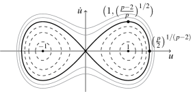
Figure 2. Curves $\tfrac{1}{2}|\dot{u}|^{2}+\frac{1}{p}\mathopen{|}u\mathclose{|}^{p}-\frac{1}{2}u^{2}=\text{const}$.

As soon as an $L^{\infty}$ estimate holds true, we essentially have a bound in any topology by help of a standard bootstrap argument. The main feature is that the bound explicitly depends on ${p}$ and does only blow up as $p\to\infty$.

Corollary 2.5.

For every $k\geqslant 0$ and $q\geqslant 1$, there exists $C>0$ such that if $u$ is a classical radial solution of Problem ($\mathcal{P}_{R,p}$) satisfying $u(0)<1$, then

$$\mathopen{\|}u\mathclose{\|}_{W^{k,q}}\leqslant C^{p-1}.$$

Proof.

Since $u(r)\leqslant C$ for any $r\geqslant 0$, we infer that

$$\Bigl{(}\int_{\Omega}\bigl{|}u^{p-1}\bigr{|}^{q}\Bigr{)}^{1/q}\leqslant\mathopen{|}\Omega\mathclose{|}^{1/q}C^{p-1}.$$

It follows from elliptic regularity (see [52, Lemma 2.2]) that for every $q>1$, there exists $K>0$ such that $\mathopen{\|}u\mathclose{\|}_{W^{2,q}}\leqslant K^{p-1}$ and the proof follows by induction. ∎

To handle Problem ($\mathcal{P}_{\varepsilon}$), we need to extend the previous bounds to this case.

Proposition 2.6.

Assume $f$ is of class $\mathcal{C}^{k}$, $k\geqslant 0$, and ($F_{2}$) holds. For any $q\geqslant 1$ and any $\varepsilon_{0}>0$, there exists $C>0$ such that if $u$ is a classical radial solution of Problem ($\mathcal{P}_{\varepsilon}$) with $u(0)\leqslant u_{0}$ and $\varepsilon\leqslant\varepsilon_{0}$, then

$$\mathopen{\|}u\mathclose{\|}_{W^{k+2,q}}\leqslant\varepsilon^{-1}C.$$

Proof.

The equation writes

$$-\varepsilon\Bigl{(}u^{\prime\prime}+\frac{N-1}{r}u^{\prime}\Bigr{)}+u=f(u).$$

Arguing as in the proof of Theorem 2.4 and using assumption ($F_{2}$), one deduces that

$$\varepsilon\frac{|u^{\prime}(r)|^{2}}{2}+F(u(r))-\frac{u^{2}(r)}{2}\leqslant F(u(0))-\frac{u^{2}(0)}{2}\leqslant M,$$

where $M:=\max_{s\in[0,u_{0}]}\bigl{(}F(s)-\frac{s^{2}}{2}\bigr{)}$. Since

$$\varliminf_{s\to+\infty}\Bigl{(}F(s)-\frac{s^{2}}{2}\Bigr{)}>M,$$

it follows that there exists a constant $L>0$ such that

$$u(r)\leqslant\max_{r\in\mathopen{[}0,R]}u(r)\leqslant L.$$

As $f$ is continuous, there exists $K>0$, depending on $\varepsilon_{0}$, such that

$$\biggl{(}\int_{\Omega}\Bigl{|}\frac{f(u)-(1-\varepsilon)u}{\varepsilon}\Bigr{|}^{q}\biggr{)}^{1/q}\leqslant\varepsilon^{-1}|\Omega|^{1/q}K.$$

Since $\varepsilon(-\Delta u+u)=f(u)-(1-\varepsilon)u$, it follows from elliptic regularity (see [52, Lemma 2.2]) that for every $q>1$, there exists $C>0$ independent of $\varepsilon$ such that

$$\mathopen{\|}u\mathclose{\|}_{W^{2,q}}\leqslant\varepsilon^{-1}C$$

and the proof follows by induction. ∎

The next lemma is in the spirit of [38, Lemma 3.5]. It will be useful in the bifurcation analysis.

Lemma 2.7.

Assume $f$ is continuous, ($F_{0}$), and ($F_{2}$) holds. Then there exists $\overline{\varepsilon}>0$ such that if $u$ is a non constant nonnegative classical radial solution of Problem ($\mathcal{P}_{\varepsilon}$) with $\varepsilon\geqslant\overline{\varepsilon}$, then $u(0)>u_{0}$.

Proof.

Assume by contradiction that $u(0)\leqslant u_{0}$ and $u$ is not constant. Proposition 2.6 implies that $u$ is uniformly bounded for $\varepsilon\geqslant 1$. Writting $u=\bar{u}+\tilde{u}$ and multiplying the equation by $\tilde{u}$, we get

$$\varepsilon\int_{B_{R}}|\nabla\tilde{u}|^{2}+\int_{B_{R}}|\tilde{u}|^{2}=\int_{B_{R}}f(u)\tilde{u}.$$

Since $u$ is a priori bounded, we infer that there exists $C>0$ such that

$$\varepsilon\int_{B_{R}}|\nabla\tilde{u}|^{2}\leqslant C\int_{B_{R}}|\tilde{u}|^{2},$$

which obviously implies that $\tilde{u}=0$ when $\varepsilon>\lambda_{2}/C$, whence a contradiction. ∎

3. Bifurcation analysis

Since $u$ is a solution of ($\mathcal{P}_{\lambda,p}$) on $\Omega$ iff $x\mapsto\lambda^{-1/(p-2)}u(x/\sqrt{\lambda})$ solves ($\mathcal{P}_{1,p}$) on $\Omega_{\lambda}:=\{\sqrt{\lambda}x\mid x\in\Omega\}$, we can fix $\lambda=1$ so that $u=1$ is a solution of ($\mathcal{P}_{\lambda,p}$). We consider the solvability of

$$\left\{\begin{aligned} -\Delta u+u&=\mathopen{|}u\mathclose{|}^{p-2}u,&&\text{ in }\Omega,\\ \partial_{\nu}u&=0,&&\text{ on }\partial\Omega,\end{aligned}\right. \mathcal{P}_{1,p}$$ ()

and we will check the positivity of the solutions a posteriori. The solutions to Problem ($\mathcal{P}_{1,p}$) with $2<p<2^{*}$ can be seen as the zeros of the Fréchet differential of the functional

$$\mathcal{E}_{p}:H^{1}(\Omega)\to\mathbb{R}:u\mapsto\frac{1}{2}\int_{\Omega}\mathopen{|}\nabla u\mathclose{|}^{2}+u^{2}-\frac{1}{p}\int_{\Omega}\mathopen{|}u\mathclose{|}^{p},$$

i.e., the zeros of the map

$$H^{1}(\Omega)\to(H^{1}(\Omega))^{\prime}:u\mapsto{{\mathcal{E}}}_{p}^{\prime}(u),$$

where the linear map ${{\mathcal{E}}}_{p}^{\prime}(u):H^{1}(\Omega)\to\mathbb{R}:h\mapsto{{\mathcal{E}}}_{p}^{\prime}(u)[h]$ is given by

$${{\mathcal{E}}}_{p}^{\prime}(u)[h]=\int_{\Omega}\nabla u\nabla h+uh-\int_{\Omega}\mathopen{|}u\mathclose{|}^{p-2}uh.$$

We consider $p$ as a unknown in the problem and we investigate the bifurcation points along the trivial solution curve $\{(p,1):p>2\}\subseteq\mathbb{R}^{+}\times H^{1}(\Omega)$ to ($\mathcal{P}_{1,p}$). We recall that a point $(p^{*},1)$ is called a bifurcation point if every punctured neighborhood of $(p^{*},1)$ contains a solution of ($\mathcal{P}_{1,p}$). The Implicit Function Theorem implies that if $(p^{*},1)$ is a bifurcation point, then the map

$$H^{1}(\Omega)\to(H^{1}(\Omega))^{\prime}:\varphi\mapsto{{\mathcal{E}}}_{p^{*}}^{\prime\prime}(1)[\varphi,\_],$$

where ${{\mathcal{E}}}_{p^{*}}^{\prime\prime}(1)[\varphi,\_]:H^{1}(\Omega)\to\mathbb{R}:\psi\mapsto{{\mathcal{E}}}_{p^{*}}^{\prime\prime}(1)[\varphi,\psi]$ is given by

$${{\mathcal{E}}}_{p^{*}}^{\prime\prime}(1)[\varphi,\psi]=\int_{\Omega}\nabla\varphi\nabla\psi+(2-p^{*})\int_{\Omega}\varphi\psi,$$

is not an isomorphism. This is the case if and only if

$$p^{*}=2+\lambda_{i}(\Omega),\qquad\text{for some }i>1,$$ (3.1)

where $0=\lambda_{1}(\Omega)<\lambda_{2}(\Omega)<\cdots$ are the eigenvalues of the operator $-\Delta$ with Neumann boundary conditions in $\Omega$.

Thanks to the fact that the problem has a variational structure, the converse is also true [9, 37, 46, 57], see also [16, 47]. Namely, if $p^{*}$ satisfies (3.1), then $(p^{*},1)$ is a bifurcation point. Moreover, standard arguments in degree theory imply that there is actually a continuum of nontrivial solutions when the dimension of the eigenspace for $\lambda_{i}(\Omega)$ is odd. A continuum $B$ of nontrivial solutions which cannot be extended (i.e., a connected component) is called a branch. If $\overline{B}\ni(2+\lambda_{i},1)$, we say that $B$ bifurcates from $(2+\lambda_{i},1)$. In this case, Rabinowitz’s principle [58] applies: a branch $B$ bifurcating from $(2+\lambda_{i},1)$ is unbounded in $\mathbb{R}\times H^{1}$ or there exists an eigenvalue $\lambda_{j}\neq\lambda_{i}$ such that $(2+\lambda_{j},1)\in\overline{B}$ (in which case we say that the branch is linked by pair).

In order to be able to establish more properties of the bifurcating branches, we now restrict ourselves to the case where $\Omega$ is a ball $B_{R}$ of radius $R$. Then, one has a precise knowledge of the eigenspaces of $-\Delta$ which makes the analysis much simpler.

We already know that the first eigenvalue $\lambda_{1}$ equals $1$ and any associated eigenfunction is constant. Let $r=\mathopen{|}x\mathclose{|}$ and $\theta=\frac{x}{\mathopen{|}x\mathclose{|}}\in\mathbb{S}^{N-1}$. By the method of separation of variables, one concludes that all eigenfunctions of $-\Delta$ with Neumann boundary conditions have the form

$$u(x)=r^{-\frac{N-2}{2}}J_{\nu}(\sqrt{\lambda_{i}}r)P_{k}\Bigl{(}\frac{x}{\mathopen{|}x\mathclose{|}}\Bigr{)},\qquad\text{where }\nu=k+\frac{N-2}{2},$$ (3.2)

$J_{\nu}$ is the Bessel function of the first kind of order $\nu$, and $P_{k}:\mathbb{R}^{N}\to\mathbb{R}$ is an harmonic homogenous polynomial of degree $k$ for some $k\in\mathbb{N}$. To satisfy the boundary conditions, the corresponding eigenvalue $\lambda_{i}\geqslant 0$ of $-\Delta$ must be such that $\sqrt{\lambda_{i}}R$ is a root of the map

$$z\mapsto(k-\nu)J_{\nu}(z)+z\partial J_{\nu}(z)=kJ_{\nu}(z)-zJ_{\nu+1}(z).$$

In other words, each of the infinitely many real roots $z_{k,\ell}$, $\ell\geqslant 1$, of this function gives rise to the eigenvalue $z_{k,\ell}^{2}/R^{2}$ of $-\Delta$. Radial eigenfunctions correspond to $k=0$. For each eigenspace $E_{i}$, the dimension of its intersection with radial functions is $0$ or $1$. Moreover, for functions in $E_{i}$ with $k=0$, one notices that the zeros of those functions are simple.

The remaining of this section is devoted to the study of radial bifurcations. We say that $(p^{*},1)$ is a radial bifurcation point if every punctured neighborhood of $(p^{*},1)$ contains radial solutions. In the sequel, we denote by $0=\lambda^{\text{rad}}_{1}<\lambda^{\text{rad}}_{2}<\lambda^{\text{rad}}_{3}<\cdots$ the eigenvalues of $-\Delta$ whose eigenspaces contain radial eigenfunctions.

3.1. Radial bifurcations in $\mathcal{C}^{2,\alpha}$

For $k\geqslant 0$, we denote by $\mathcal{C}^{k,\alpha}_{\textup{rad}}(\bar{B}_{R})$ the space $\mathcal{C}^{k,\alpha}(\bar{B}_{R})$ restricted to radially invariant functions and

$$\tilde{\mathcal{C}}^{2,\alpha}_{\textup{rad}}(\bar{B}_{R}):=\bigl{\{}u\in\mathcal{C}^{2,\alpha}_{\textup{rad}}(\bar{B}_{R})\bigm{|}\partial_{r}u(R)=0\bigr{\}}.$$

If we define $-\Delta$ on the space $\tilde{\mathcal{C}}^{2,\alpha}_{\textup{rad}}(\bar{B}_{R})$, then the spectrum is made of the increasing sequence $0=\lambda^{\text{rad}}_{1}<\lambda^{\text{rad}}_{2}<\lambda^{\text{rad}}_{3}<\cdots$ of simple eigenvalues.

The function $u\in\tilde{\mathcal{C}}^{2,\alpha}_{\text{rad}}$ is a classical solution of Problem ($\mathcal{P}_{1,p}$) with $\Omega=B_{R}$ if and only if the couple $(p,u)$ is a zero of the function

$$F:\mathbb{R}\times\tilde{\mathcal{C}}^{2,\alpha}_{\text{rad}}\to{\mathcal{C}}^{0,\alpha}_{\text{rad}}:(p,u)\mapsto(-\Delta+\operatorname{\mathbbm{1}})u-\mathopen{|}u\mathclose{|}^{p-2}u.$$ (3.3)

It is easily seen that

$$\partial_{u}F(2+\lambda_{i},1)[v]=(-\Delta+\operatorname{\mathbbm{1}})v-\lambda_{i}v,$$ (3.4)

so that classical bifurcation theory implies that if $E_{i}\cap\tilde{\mathcal{C}}^{2,\alpha}_{\text{rad}}=\{0\}$, then $(2+\lambda_{i},1)$ is not a radial bifurcation point in $\tilde{\mathcal{C}}^{2,\alpha}_{\textup{rad}}$ whereas if $E_{i}\cap\tilde{\mathcal{C}}^{2,\alpha}_{\text{rad}}\neq\{0\}$, then $(2+\lambda_{i},1)$ is a bifurcation point in $\tilde{\mathcal{C}}^{2,\alpha}_{\textup{rad}}$. We will improve this first vague result by studying the local behavior of the bifurcations branches from $(2+\lambda^{\text{rad}}_{i},1)$ in $\tilde{\mathcal{C}}^{2,\alpha}$. We will use the celebrated Crandall-Rabinowitz theorem [20, Theorem 1.7 and 1.18] (see also [6]) in a form that we recall first.

Proposition 3.1 (Crandall-Rabinowitz).

Let $X$ and $Y$ be two Banach spaces, $p^{*}\in\mathbb{R}$ and $u^{*}\in X$. Assume $F:\mathbb{R}\times X\to Y:(p,u)\mapsto F(p,u)$ is such that

1. $F(p,u^{*})=0$ for any $p$ in a neighborhood of $p^{*}$;

2. the partial derivatives $\partial_{p}F$, $\partial_{u}F$ and $\partial_{pu}F$ exist and are continuous in a neighborhood of $(p^{*},u^{*})$;

3. $\ker\bigl{(}\partial_{u}F(p^{*},u^{*})\bigr{)}$ is one-dimensional and is thus spanned by some $\varphi^{*}\in X\setminus\{0\}$;

4. $\operatorname{Im}\bigl{(}\partial_{u}F(p^{*},u^{*})\bigr{)}$ has codimension $1$ and is thus the kernel $\{y\in Y:\langle\psi,y\rangle=0\}$ of some continuous linear functional $\psi:Y\to\mathbb{R}$.

Then the following assertions hold.

1. If

   $$a:=\langle\psi,\partial_{pu}F(p^{*},u^{*})[\varphi^{*}]\rangle\neq 0,$$

   then $(p^{*},u^{*})$ is a bifurcation point for $F$. In addition, the set of nontrivial solutions of $F=0$ in a neighborhood of $(p^{*},u^{*})$ is given by a unique continuous curve $s\mapsto(\bar{p}(s),\bar{u}(s))$ defined for $s$ close to $0$. More precisely $(\bar{p}(0),\bar{u}(0))=(p^{*},u^{*})$, $\bar{u}$ is of class $\mathcal{C}^{1}$, $\partial_{s}\bar{u}(0)=\varphi^{*}$, and, for all $(p,u)$ in a neiborhood of $(p^{*},u^{*})$,

   $$\bigl{(}F(p,u)=0\land u\neq u^{*}\bigr{)}\Leftrightarrow\exists\,s\neq 0,\ \linebreak[2](p,u)=(\bar{p}(s),\bar{u}(s)).$$

   If $\partial_{u}^{2}F$ exists and is continuous, the curve is of class $\mathcal{C}^{1}$.

2. Assuming $a\neq 0$, if $\partial^{2}_{u}F$ is continuous and

   $$b:=-\frac{1}{2a}\bigl{\langle}\psi,\partial^{2}_{u}F(p^{*},u^{*})[\varphi^{*},\varphi^{*}]\bigr{\rangle}\neq 0,$$

   then the bifurcation point is transcritical and the nontrivial solution curve can be (locally) written $(p,u_{p})$ with

   $$u_{p}=u^{*}+\frac{p-p^{*}}{b}\varphi^{*}+o(p-p^{*}).$$ (3.5)

3. Assuming $a\neq 0$, $b=0$ and $\partial^{3}_{u}F$ is continuous, if

   $$c:=-\frac{1}{6a}\Bigl{(}\bigl{\langle}\psi,\partial_{u}^{3}F(p^{*},u^{*})[\varphi^{*},\varphi^{*},\varphi^{*}]\bigr{\rangle}+3\bigl{\langle}\psi,\partial_{u}^{2}F(p^{*},u^{*})[\varphi^{*},w]\bigr{\rangle}\Bigr{)}\neq 0,$$

   where $w\in X$ is any solution of the equation $\partial_{u}F(p^{*},u^{*})[w]=-\partial^{2}_{u}F(p^{*},u^{*})[\varphi^{*},\varphi^{*}],$ we have

   $$u_{p}=u^{*}\pm\Bigl{(}\frac{p-p^{*}}{c}\Bigr{)}^{1/2}\varphi^{*}+o\bigl{(}{\mathopen{|}p-p^{*}\mathclose{|}}^{1/2}\bigr{)}.$$

   In particular, the bifurcation point is supercritical if $c>0$ and subcritical if $c<0$.

Figure 3. Type of bifurcations.

We now apply these statements to our problem. We still consider the map (3.3). We fix $(p^{*},u^{*})=(2+\lambda^{\text{rad}}_{i},1)$. Assumption (i) is clear while (ii) can be checked with standard arguments. We deduce from (3.4) that

$$\ker\bigl{(}\partial_{u}F(2+\lambda^{\text{rad}}_{i},1)\bigr{)}=\langle\varphi_{i}\rangle,$$

where we can assume that $\varphi_{i}$ is the unique radial eigenvalue of $-\Delta$ associated to $\lambda^{\text{rad}}_{i}$, normalized in $L^{2}(B_{R})$. By the Fredholm alternative, we also have

$$\operatorname{codim}\bigl{(}\operatorname{Im}(\partial_{u}F(2+\lambda^{\text{rad}}_{i},1))\bigr{)}=1$$

and $f\in\operatorname{Im}\bigl{(}\partial_{u}F(2+\lambda^{\text{rad}}_{i},1)\bigr{)}$ if and only if $\int_{B_{R}}f\varphi_{i}=0$, so that one can take

$$\psi:{\mathcal{C}}^{0,\alpha}_{\text{rad}}\to\mathbb{R}:f\mapsto\langle\psi,f\rangle:=\int_{B_{R}}f\varphi_{i}.$$

Simple computations show that

$$a=\int_{B_{R}}\partial_{pu}F(2+\lambda^{\text{rad}}_{i},1)[\varphi_{i}]\varphi_{i}=-\int_{B_{R}}\varphi_{i}^{2}=-1$$ (3.6)

and

$$b=-\frac{1}{2a}\int_{B_{R}}\partial^{2}_{u}F(2+\lambda^{\text{rad}}_{i},1)[\varphi_{i},\varphi_{i}]\varphi_{i}\,{\mathrm{d}}x=-\frac{1}{2}(1+\lambda^{\text{rad}}_{i})\lambda^{\text{rad}}_{i}\int_{B_{R}}\varphi_{i}^{3}.$$ (3.7)

In order to compute $b$, we will use the following property of Bessel’s functions which is in fact the key in our analysis.

Lemma 3.2.

Let $\nu\geqslant 1/2$, $\beta>0$ and $\alpha\in\mathopen{]}-1-\nu\beta,\beta/2\mathclose{]}$. If $\nu=1/2$, assume further that $\alpha<\beta/2$. Then for every $x>0$, we have

$$\int_{0}^{x}s^{\alpha}J_{\nu}^{\beta}(s)\,{\mathrm{d}}s>0,$$ (3.8)

where $J_{\nu}^{\beta}(s)$ means $\operatorname{sign}\bigl{(}J_{\nu}(s)\bigr{)}\mathopen{|}J_{\nu}(s)\mathclose{|}^{\beta}$.

Proof.

First note that the integral exists. Indeed, since $J_{\nu}(x)$ behaves like $x^{-\nu}$ as $x\to 0$, the integrant is integrable in a neighborhood of $0$ iff $\alpha+\nu\beta>-1$.

Next, recall that, for $\nu\geqslant 0$, the following representation of Bessel functions holds :

$$\forall x>0,\qquad J_{\nu}(x)=\sqrt{\frac{2}{\pi x}}\,\sqrt{p_{\nu}(x)}\sin\biggl{(}\int_{0}^{x}\frac{\mathrm{d}\xi}{p_{\nu}(\xi)}\biggr{)},$$ (3.9)

where

$$p_{\nu}(x):=\tfrac{1}{2}\pi x\bigl{(}J_{\nu}^{2}(x)+Y_{\nu}^{2}(x)\bigr{)}.$$

According to formulas (10.18.4), (10.18.6) and (10.18.8) of [55], we have

$$J_{\nu}(x)=M_{\nu}(x)\cos\bigl{(}\theta_{\nu}(x)\bigr{)},$$

where $p_{\nu}(x)=\tfrac{1}{2}\pi xM_{\nu}^{2}(x)>0$ and $\partial_{x}\theta_{\nu}(x)=1/p_{\nu}(x)$. Given that

$$\theta_{\nu}(x)\to-\tfrac{1}{2}\pi,\ \text{ as }x\xrightarrow{>}0,$$

one deduces that $\theta_{\nu}(x)=-\tfrac{1}{2}\pi+\int_{0}^{x}{1}/{p_{\nu}(\xi)}\,{\mathrm{d}}\xi$, hence the claimed formula (we also refer to [41]).

Now, note that the formulas (10.7.8) in [55] imply that

$$\lim_{x\to+\infty}p_{\nu}(x)=1,$$

whence

$$\lim_{x\to+\infty}\int_{0}^{x}{1}/{p_{\nu}(\xi)}\,{\mathrm{d}}\xi=+\infty.$$

Using (3.9) and performing the change of variables $t=\int_{0}^{x}{1}/{p_{\nu}(\xi)}\,{\mathrm{d}}\xi$, the claim (3.8) can be written

$$\forall\tau>0,\qquad\int_{0}^{\tau}\bigl{(}X(t)\bigr{)}^{\alpha-\beta/2}\bigl{(}p_{\nu}(X(t))\bigr{)}^{1+\beta/2}\sin^{\beta}(t)\,{\mathrm{d}}t>0$$

where $X:\mathopen{[}0,+\infty\mathclose{[}\to\mathopen{[}0,+\infty\mathclose{[}$ is such that $X(0)=0$ and $\partial_{t}X(t)=p_{\nu}(X(t))>0$. Since the sine function is periodic, it is enough to show that $t\mapsto(X(t))^{\alpha-\beta/2}p_{\nu}^{1+\beta/2}(X(t))$ is decreasing because then the integral on the interval $\mathopen{[}2k\pi,(2k+1)\pi\mathclose{]}$ will be greater than the negative contribution in the next interval $\mathopen{[}2(k+1)\pi,(2k+2)\pi\mathclose{]}$. As the function $X$ is increasing, it is equivalent to show that $x\mapsto x^{\alpha-\beta/2}\bigl{(}p_{\nu}(x)\bigr{)}^{1+\beta/2}$ is decreasing, or, setting $\gamma=(\alpha-\beta/2)/(1+\beta/2)$, that $x\mapsto x^{\gamma}p_{\nu}(x)$ is decreasing.

According to formula (10.9.30) of [55], we have

$$p_{\nu}(x)=\tfrac{4}{\pi}x\int_{0}^{\infty}\cosh(2\nu t)K_{0}(2x\sinh t)\,{\mathrm{d}}t$$ (3.10)

where $K_{0}$ is the second modified Bessel function. We have to distinguish between $\nu>1/2$ and $\nu=1/2$.

Assume first $\nu>1/2$. Performing the change of variable $s:=x\sinh t$ in (3.10), we get

$$p_{\nu}(x)=\tfrac{4}{\pi}\int_{0}^{\infty}\frac{\cosh(2\nu t)}{\cosh t}\Bigr{|}_{t=\operatorname{arcsinh}(s/x)}K_{0}(2s)\,{\mathrm{d}}s.$$

The function $t\mapsto{\cosh(2\nu t)}/{\cosh t}$ is increasing. Therefore the first term of the product is a decreasing function of $x$. As $K_{0}>0$, so is $p_{\nu}$. It is therefore sufficient that $\gamma\leqslant 0$ in this case.

If $\nu=1/2$, $p_{\nu}(x)=1$ for all $x>0$ (see e.g. (10.43.18) in [55]). It follows that the map $x\mapsto x^{\gamma}p_{\nu}(x)$ is decreasing iff $\gamma<0$. ∎

Remark 3.3.

When $\nu=1/2$ (i.e., $N=3$ for our application in upcoming Theorem 3.5), $J_{\nu}(x)=\sqrt{2/(\pi x)}\sin x$ and so the statement simplifies to

$$\forall x>0,\qquad\int_{0}^{x}x^{\alpha-\beta/2}\sin^{\beta}(x)\,{\mathrm{d}}x>0$$

which is true as soon as $x\mapsto x^{\alpha-\beta/2}$ is decreasing. This is the only case where the assumptions of Lemma 3.2 are sharp: for $\nu>1/2$, the statement (3.8) remains true for some $\alpha>\beta/2$.

Remark 3.4.

When $\nu=0$ (i.e., $N=2$ for our application), although $p_{0}$ is increasing and an asymptotic analysis around $0$ shows that $x^{\gamma}p_{0}(x)$ is not decreasing whatever $\gamma$, numerics indicate that (3.8) is positive at least if $\alpha<0.45\beta-0.15$, and in particular in the case of interest for Theorem 3.5: $\alpha=1-\nu=1$ and $\beta=3$.

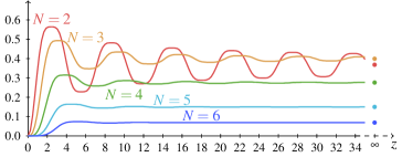
Figure 4. Plots of $z\mapsto\int_{0}^{z}s^{1-\nu}J_{\nu}^{3}(s)\,{\mathrm{d}}s$ with $\nu=N/2-1$ and $N=2,\ldots,6$.

Moreover, Equation (10.22.74) of [55] asserts

$$\int_{0}^{\infty}x^{1-\nu}J_{\nu}^{3}(x)\,{\mathrm{d}}x=\frac{2^{\nu-1}(3/16)^{\nu-1/2}}{\pi^{1/2}\,\Gamma(\nu+1/2)}>0,$$

so that the (3.8) holds true for $x$ large enough in the case $\alpha=1-\nu$ and $\beta=3$.

With Lemma 3.2 at hand, we can prove the following.

Theorem 3.5.

Assume $\Omega=B_{R}$ and $N\geqslant 3$. For every $i\geqslant 2$, $(p_{i},u_{0}):=(2+\lambda^{\text{rad}}_{i},1)$ is a bifurcation point in $\tilde{\mathcal{C}}^{2,\alpha}(B_{R})$ of Problem ($\mathcal{P}_{1,p}$). Denote $B_{i}$ the branch bifurcating from $(2+\lambda^{\text{rad}}_{i},1)$. The following holds:

1. close to $(2+\lambda^{\text{rad}}_{i},1)$, the branch is a $\mathcal{C}^{1}$-curve;

2. there exists $\varepsilon>0$ (which does not depend on $i$) such that if $(p,u_{p})\in B_{i}$ then $u_{p}$ is positive and $p>2+\varepsilon$;

3. the bifurcation point $(2+\lambda^{\text{rad}}_{i},1)$ is transcritical. Furthermore, if $B_{i}^{-}$ denotes the part of the branch starting at $(2+\lambda^{\text{rad}}_{i},1)$ which bifurcates to the right of $2+\lambda^{\text{rad}}_{i}$, we have $(p,u_{p})\in B_{i}^{-}\Rightarrow u_{p}(0)<1$, while on the part $B_{i}^{+}$ of the branch bifurcating to the left of $2+\lambda^{\text{rad}}_{i}$, the branch is made of solutions satisfying $u_{p}(0)>1$.

Observe that for $i=2$, the functions on the branch emanating to the right (resp. left) of $2+\lambda^{\text{rad}}_{2}$ are increasing (resp. decreasing), at least when $p$ is close enough to $2+\lambda^{\text{rad}}_{2}$. We will prove later on that this holds actually along the whole branch. Some parts of the proof follow from nowadays standard arguments. We give them for completeness.

Proof.

(i) Since $a\neq 0$, Crandall-Rabinowitz theorem 3.1 implies that $(2+\lambda^{\text{rad}}_{i},1)$ is a continuous bifurcation point for $F$. In addition, the set of non-trivial solutions of $F=0$ is composed locally of a unique curve of class $\mathcal{C}^{1}$. Hence (i) holds.

(ii) Let $\mathcal{B}_{i}\subseteq\mathbb{R}\times\tilde{\mathcal{C}}^{2,\alpha}_{\text{rad}}$ be the continuum that branches out from $(2+\lambda^{\text{rad}}_{i},1)$, $B_{i}:=\mathcal{B}_{i}\setminus\{(2+\lambda^{\text{rad}}_{i},1)\}$ and $(p,u)\in B_{i}$. Close to the bifurcation point $(2+\lambda^{\text{rad}}_{i},1)$, $u$ is close to $1$ in the $\mathcal{C}^{2}$ topology, so that $u$ is clearly positive. Let $\tilde{p}>2$ be given by Theorem 2.3. We can assume that $\tilde{p}$ is smaller than $2+\lambda^{\text{rad}}_{2}>2$. We claim that

$$\forall(p,u)\in B_{i},\quad p>\tilde{p}\text{ and }u>0.$$

By connectedness, if the claim does not hold, there exists, on the continuum $B_{i}$, a nonnegative solution $u$ to ($\mathcal{P}_{1,p}$) such that $p=\tilde{p}$ or $u$ vanishes at at least one point. In the first case $p=\tilde{p}$, Theorem 2.3 implies that $u\equiv 1$ or $u\equiv 0$ but this is impossible since neither $(\tilde{p},1)$ nor $(p,0)$, $p\in\mathopen{]}2,+\infty\mathclose{[}$, are bifurcation points of $F$. We can therefore suppose that $p>\tilde{p}$, $u\geqslant 0$ and $u\not\equiv 0$. If the set $\{r\in[0,R]\mid u(r)=0\}$ contains a point $r_{0}\in\mathopen{]}0,R\mathclose{]}$, then $u^{\prime}(r_{0})=0$ because $r_{0}$ is either an interior minimum or the boundary condition holds. The local uniqueness of the solution for the Cauchy problem (2.2) with initial data $u(r_{0})=0$, $u^{\prime}(r_{0})=0$ now implies $u\equiv 0$ which is a contradiction. It remains to deal with the case where $\{r\in[0,R]\mid u(r)=0\}=\{0\}$. Choose $s>0$ small enough so that $u(r)<1$ for all $r\in\mathopen{[}0,s\mathclose{]}$. We claim that $u^{\prime}>0$ on $\mathopen{]}0,s\mathclose{]}$. Because $u>0$ on $\mathopen{]}0,s\mathclose{]}$, there are points $r$ arbitrarily close to $0$ such that $u^{\prime}(r)>0$. It is thus sufficient to show that $u^{\prime}(r)\neq 0$ for $r\in\mathopen{]}0,s\mathclose{]}$. Notice that, in view of equation (2.2),

$$\text{for all }r\in\mathopen{]}0,s\mathclose{]},\ u(r)\in\mathopen{]}0,1\mathclose{[}\text{ and }u^{\prime}(r)=0\text{ implies }u^{\prime\prime}(r)>0.$$ (3.11)

Suppose that, on the contrary, $u^{\prime}$ vanishes at $t\in\mathopen{]}0,s\mathclose{]}$. Using (3.11) with $r=t$, one deduces that the maximum of $u$ over $\mathopen{[}0,t\mathclose{]}$ occurs at some interior point $r_{1}\in\mathopen{]}0,t\mathclose{[}$ such that $u^{\prime}(r_{1})=0$ and $u^{\prime\prime}(r_{1})\leqslant 0$. This contradicts (3.11) and thus we indeed have $u^{\prime}>0$ on $\mathopen{]}0,s\mathclose{]}$. Now, remember that, because $u$ describes the profile of a radial function, $u^{\prime}(0)=0$. Therefore, for all $r\in\mathopen{[}0,R\mathclose{]}$, $h(r)\leqslant h(0)=0$ where $h$ is defined by (2.4). This implies

$$(u^{\prime})^{2}\leqslant u^{2}-\tfrac{2}{p}u^{p}\leqslant u^{2}$$

and thus $u^{\prime}\leqslant u$ on $\mathopen{]}0,s\mathclose{[}$. Using Gronwall’s inequality, one concludes $u(r)\geqslant u(s)\operatorname{e}^{r-s}$ for all $r\in\mathopen{[}0,s\mathclose{]}$ which is a contradiction when $r=0$.

(iii) The bifurcation is transcritical if $b\neq 0$, where $b$ is defined by (3.7). Taking the explicit form of the eigenfunctions, and integrating in spherical coordinates, one finds that $b\neq 0$ if and only if

$$\int_{0}^{R}\Bigl{(}r^{-\frac{N-2}{2}}J_{\nu}\bigl{(}r\sqrt{\bar{\lambda}_{i}}/R\bigr{)}\Bigr{)}^{3}r^{N-1}\,{\mathrm{d}}r\neq 0,$$

or equivalently

$$\int_{0}^{\sqrt{\bar{\lambda}_{i}}}t^{1-\nu}J_{\nu}^{3}(t)\,{\mathrm{d}}t\neq 0,$$ (3.12)

where $\bar{\lambda}_{i}=\lambda^{\text{rad}}_{i}(B_{1})$ is the corresponding spherical eigenvalue of $-\Delta$ on the unit ball (so that $\lambda^{\text{rad}}_{i}=\bar{\lambda}_{i}/R^{2}$) and $\nu=N/2-1\geqslant 0$. According to Lemma 3.2 with $\alpha=1-\nu$ and $\beta=3$, this integral is positive for all $i$. Recalling that

$$b=-\frac{1}{2}(1+\lambda^{\text{rad}}_{i})\lambda^{\text{rad}}_{i}\,\mathopen{|}\mathbb{S}^{N-1}\mathclose{|}\int_{0}^{\sqrt{\bar{\lambda}_{i}}}t^{1-\nu}J_{\nu}^{3}(t)\,{\mathrm{d}}t,$$

one gets $b<0$ for all $i$.

For the last statement in (iii), first notice that, up to a positive normalization factor, the function $\varphi_{i}$ is $x\mapsto\mathopen{|}x\mathclose{|}^{-\nu}J_{\nu}(\sqrt{\lambda^{\text{rad}}_{i}}\mathopen{|}x\mathclose{|})$. In view of equation (10.7.3) of [55], $\varphi_{i}(0)>0$. Using the fact that $b<0$ and the asymptotic expansion of the branches (3.5), one concludes that, in a neighborhood of $(2+\lambda^{\text{rad}}_{i},1)$, the functions on the branch emanating to the right (resp. left) of $2+\lambda^{\text{rad}}_{i}$ satisfy $u(0)<1$ (resp. $u(0)>1$). This property remains true along the whole branch. Indeed, since the function $h$ defined by (2.3) is non-increasing, one sees that $u(0)\neq 1$ otherwise $u$ is the constant solution $u\equiv 1$ which does not belong to the branch $B_{i}$. ∎

Remark 3.6.

In contrast with Theorem 3.5, the bifurcation points for the one-dimensional case are always supercritical. On $B_{R}=\mathopen{]}-R,R\mathclose{[}$, all eigenvalues are simple. Let $\varphi_{i}$ be a $i$ th eigenfunction, sorted so that the corresponding eigenvalues $\lambda_{i}$ are increasing, and normalized so that $\mathopen{\|}\varphi_{i}\mathclose{\|}_{L^{2}}=1$. As before, we take $\langle\psi,v\rangle:=\int_{B_{R}}v\varphi_{i}$. Elementary but tedious computations then show that

$$a=-\int_{-R}^{R}\varphi_{i}^{2}=-1\neq 0,\quad b=-\frac{1}{2}(1+\lambda_{i})\lambda_{i}\int_{-R}^{R}\varphi_{i}^{3}=0$$

and

$$c=\tfrac{-1}{6a}(1+\lambda_{i})\lambda_{i}\Bigl{(}-(\lambda_{i}-1)\int_{-R}^{R}\varphi_{i}^{4}-3(1+\lambda_{i})\lambda_{i}\int_{-R}^{R}\varphi_{i}^{2}w\Bigr{)}=\frac{\pi^{2}i^{2}}{12\,R^{3}}+\frac{5\pi^{4}i^{4}}{192\,R^{5}}+\frac{\pi^{6}i^{6}}{768\,R^{7}}$$

where $w$ is any solution of $-w^{\prime\prime}-\lambda_{i}w=\varphi_{i}^{2}$ with Neumann boundary conditions.

When $N=2$, we conjecture Theorem 3.5 remains but we have to leave that as an open question for which a positive answer is strongly supported by the numerical computations. We can state the following weaker result.

Theorem 3.7.

Assume $\Omega=B_{R}$ and $N=2$. For every $i\geqslant 2$, $(p_{i},u_{0}):=(2+\lambda^{\text{rad}}_{i},1)$ is a bifurcation point in $\tilde{\mathcal{C}}^{2,\alpha}(B_{R})$ of Problem ($\mathcal{P}_{1,p}$). Denote $B_{i}$ the branch bifurcating from $(2+\lambda^{\text{rad}}_{i},1)$. The following holds:

1. close to $(2+\lambda^{\text{rad}}_{i},1)$, the branch is a $\mathcal{C}^{1}$-curve;

2. there exists $\varepsilon>0$ (which does not depend on $i$) such that if $(p,u_{p})\in B_{i}$ then $u_{p}$ is positive and $p>2+\varepsilon$;

3. in addition to the point $(2+\lambda^{\text{rad}}_{i},1)$, the branch is composed of two connected components, one along which $u(0)<1$ and another one along which $u(0)>1$;

4. if $i$ is large enough, then the bifurcation from $(2+\lambda^{\text{rad}}_{i},1)$ is transcritical and the characterization of the branch stated in assertion (iii) of Theorem 3.5 holds.

Proof.

The first two assertions follow as in the proof of Theorem 3.5. Assertion (iv) is a consequence of Remark 3.4. Finally, Theorem 3.1 asserts that the curve $s\mapsto(\bar{p}(s),\bar{u}(s))$ locally giving the bifurcation branch around $(2+\lambda^{\text{rad}}_{i},1)$ is such that

$$\bar{u}(s)=1+s\varphi_{i}+\operatorname{o}(s)$$

where $\varphi_{i}$ can be chosen so that $\varphi_{i}(0)>0$. Thus, $u(0)>1$ when $s>0$ and $u(0)<1$ when $s<0$. The same argument as for Theorem 3.5 implies that these properties are preserved along the corresponding continuums. ∎

3.2. Properties of the solutions along the branches

In this subsection, we first show that the branches $B_{i}$ are unbounded and that they do not cross. We introduce the following definition which is intended to distinguish the solutions bifurcating at $(2+\lambda^{\text{rad}}_{i},1)$.

Definition 3.8.

A positive radial solution $u$ is of type $i$ if and only if the number of zeros of $r\mapsto u(r)-1$ is the same as the number of zeros of ${\varphi}_{i}$, the radial eigenfunction associated to $\lambda^{\text{rad}}_{i}$. If $u$ is of type $i$ and $u(0)>1$ then we say that $u$ is of type $i_{+}$ while if $u(0)<1$, we say that $u$ is of type $i_{-}$.

The next proposition states the classical separation of the branches via nodal properties.

Proposition 3.9.

The branches $B_{i}\subseteq\mathbb{R}\times\bigl{(}\mathcal{C}_{\text{rad}}^{2,\alpha}\setminus\{1\}\bigr{)}$ starting from $(2+\lambda^{\text{rad}}_{i},1)$ ($i>1$) are unbounded for the $\mathcal{C}_{\text{rad}}^{2,\alpha}$-topology and do not intersect. Moreover, along the branch $B_{i}$, the solutions of ($\mathcal{P}_{1,p}$) are of type $i$.

Proof.

We know that the branches are unbounded in $\mathbb{R}\times\mathcal{C}_{\text{rad}}^{2,\alpha}$ or linked by pair. To disprove the second possibility, it is enough to prove that along $B_{i}$, the solutions are of type $i$. Let $(p,u)\in B_{i}$. We know that $p>2+\varepsilon$ and as observed in the proof of statement (iii) of Theorem 3.5, $u(0)\neq 1$. Moreover, as $u$ is a solution of the ODE

$$-\partial_{r}^{2}u-\frac{N-1}{r}\partial_{r}u+u=\mathopen{|}u\mathclose{|}^{p-2}u,$$ (3.13)

which also possesses the constant solution $1$, the roots of $u-1$ are simple. Therefore, the number of roots of $u-1$ along the $\mathcal{C}^{2,\alpha}$-continuum $B_{i}$ cannot change. To prove that the number of roots of $u-1$ is the same as $\varphi_{i}$, we consider a sequence $\bigl{(}(p_{n},u_{n})\bigr{)}_{n}\subseteq B_{i}$ converging to $(2+\lambda^{\text{rad}}_{i},1)$ in $\mathbb{R}\times\mathcal{C}^{2,\alpha}$ and we set $v_{n}:=(u_{n}-1)/\mathopen{\|}u_{n}-1\mathclose{\|}_{\mathcal{C}^{2,\alpha}}$. Due to the fact that the embedding $\mathcal{C}^{2,\alpha}\hookrightarrow\mathcal{C}^{0,\alpha}$ is compact, one can assume that $v_{n}\to v^{*}$ in $\mathcal{C}^{0,\alpha}$. Recalling that $u_{n}>0$, the equation for $v_{n}$ can be written as

$$v_{n}=(-\Delta+\operatorname{\mathbbm{1}})^{-1}\frac{u_{n}^{p_{n}-1}-1}{\mathopen{\|}u_{n}-1\mathclose{\|}_{\mathcal{C}^{2,\alpha}}}=(-\Delta+\operatorname{\mathbbm{1}})^{-1}\bigl{(}(1+\lambda^{\text{rad}}_{i}+o(1))v_{n}+O(\mathopen{\|}u_{n}-1\mathclose{\|}_{\mathcal{C}^{0,\alpha}})\bigr{)}.$$

Since the inverse of the $-\Delta+\operatorname{\mathbbm{1}}$ is continuous, one deduces that the convergence $v_{n}\to v^{*}$ actually occurs in $\mathcal{C}^{2,\alpha}$, thus $\mathopen{\|}v^{*}\mathclose{\|}_{\mathcal{C}^{2,\alpha}}=1$ and $v^{*}$ is a radial eigenfunction of $-\Delta$ with eigenvalue $\lambda^{\text{rad}}_{i}$. By simplicity, $v^{*}$ is a multiple of $\varphi_{i}$ and has the same number of zeros. Since these zeros are simple, $v_{n}$ also has the same number of zeros as $v^{*}$ for $n$ large. This completes the proof. ∎

Summing up the previous results, we can distinguish the behavior of the solutions on the two connected components of the branch $B_{i}$.

Theorem 3.10.

Let $N\geqslant 3$. The set $B_{i}$ consists of two branches $B_{i}^{\pm}$ such that

1. on $B_{i}^{-}$, $p>2+\lambda^{\text{rad}}_{i}$ close to the bifurcation point, the solutions $u$ are of type $i_{-}$, $u(0)$ is a global minimum, $u$ has exactly $i$ critical points which are all non degenerate local extrema, each maxima (resp. minima) being strictly greater (resp. smaller) than $1$ and strictly smaller (resp. larger) than the previous one;

2. on $B_{i}^{+}$, $p<2+\lambda^{\text{rad}}_{i}$ close to the bifurcation point, the solutions $u$ are of type $i_{+}$, $u(0)$ is a global maximum, $u$ has exactly $i$ critical points which are all non degenerate local extrema, each maxima (resp. minima) being strictly greater (resp. smaller) than $1$ and strictly smaller (resp. larger) than the previous one.

Proof.

The proof is a simple consequence of the previous statements and of standard ODE arguments based on the energy dissipation (2.3). ∎

Remark 3.11.

The same result holds for $N=2$ except that we do not know how the branches $B^{\pm}_{i}$ behave for $p$ close to $2+\lambda^{\text{rad}}_{i}$.

Note that on the first bifurcation, the solutions are increasing on one part of the branch and decreasing on the other part. On the other branches, the solutions are oscillating around $1$ with a “decreasing envelope”.

3.3. Degeneracy and multiplicity

We now collect some of the consequences of the bifurcation analysis. In particular, the a priori estimates given in Section 2 lead to further qualitative results. We recall that a positive solution $u_{0}$ of ($\mathcal{P}_{1,p}$) is said to be degenerate if there exists $v\neq 0$ such that

$$\left\{\begin{aligned} -\Delta v+v&=(p-1)\mathopen{|}u_{0}\mathclose{|}^{p-2}v,&&\text{ in }\Omega,\\ \partial_{\nu}v&=0,&&\text{ on }\partial\Omega,\end{aligned}\right.$$

or, equivalently, if the kernel of $\partial_{u}F(p,u_{0})$ is larger than $\{0\}$.

Proposition 3.12.

Let $N\geqslant 3$, $\Omega=B_{R}$, and $i\geqslant 2$. If $2+\lambda^{\text{rad}}_{i}(B_{R})<2^{*}$, Problem ($\mathcal{P}_{1,p}$) admits a degenerate positive radial solution of type $i_{+}$ for some $p=p_{i}\in\mathopen{]}2,2+\lambda^{\text{rad}}_{i}\mathclose{[}$.

Proof.

We know that statement (iii) of Theorem 3.5 holds. On $B_{i}^{+}$, the branch starting from the left of $(2+\lambda^{\text{rad}}_{i},1)$, the solutions are a priori bounded as long as $p<2^{*}$ (see Proposition 2.2). On the other hand, we know that the branch is unbounded (for the topology of $\mathbb{R}\times\mathcal{C}^{2,\alpha}$) and that $p\geqslant 2+\varepsilon$ for some $\varepsilon>0$ that depends only on $R$. It follows that $p$ achieves a minimum along the continuum at some value $p_{i}\geqslant 2+\varepsilon$. If the corresponding solution $u_{p_{i}}$ was non degenerate, the Implicit Function Theorem would allow to extend the branch to the left of $p_{i}$ which is a contradiction. ∎

Observe that $\lambda^{\text{rad}}_{i}(B_{R})<2^{*}-2$ as soon as $R$ is large so that on large balls, there exist many degenerate positive solutions. These turning points on the bifurcation diagram should imply a change of Morse index (for instance in the space of radial functions) along the branches and a change in the minimax property of the solution. This is supported by the numerical computations of section 6.2. It also implies a local multiplicity result for solutions of type $i_{+}$.

Corollary 3.13.

Let $N\geqslant 3$. If $2+\lambda^{\text{rad}}_{i}(B_{R})<2^{*}$, there exists $\varepsilon_{i}>0$ such that if $2+\lambda^{\text{rad}}_{i}(B_{R})-\varepsilon_{i}<p<2+\lambda^{\text{rad}}_{i}(B_{R})$, Problem ($\mathcal{P}_{1,p}$) with $\Omega=B_{R}$ has at least two positive radial solutions of type $i_{+}$.

The numerical computations of Sections 6.2 and 6.3 indicate that $\lambda^{\text{rad}}_{i}(B_{R})-\varepsilon_{i}$ is actually the turning point $p_{i}$ from Proposition 3.12 but a proof of this fact actually requires a deeper analysis that we do not pursue here. When $2+\lambda^{\text{rad}}_{2}(B_{R})<2^{*}$, this means there exist two decreasing solutions for $p_{2}<p<2+\lambda^{\text{rad}}_{2}(B_{R})$.

In Section 6.3, we also numerically observe that the solution on the unbounded part of the branch $B^{+}_{i}$, i.e. after the turning point, explodes as $p\to 2^{*}$. The solutions seem to concentrate at the origin when $p\to 2^{*}$. It is therefore natural to conjecture that all these branches bifurcate from infinity at $p=2^{*}$.

We next derive a global multiplicity result which answers positively a conjecture in [12] at least in the case of a pure power nonlinearity (we believe that the general case can be derived with similar arguments). Indeed, assuming

1. $f\in\mathcal{C}^{1}\bigl{(}[0,+\infty),\mathbb{R}\bigr{)}$, $f(0)=0$ and $\displaystyle f^{\prime}(0)=\lim_{s\to 0^{+}}\frac{f(s)}{s}=0$;

2. $f$ is nondecreasing;

3. $\displaystyle{\liminf\limits_{s\to+\infty}\frac{f(s)}{s}>1}$ and there exists $u_{0}>0$ such that $f(u_{0})=u_{0}$ and $f^{\prime}(u_{0})>1+\lambda^{\text{rad}}_{2}$;

it is proved in [12] that the problem

$$\begin{cases}-\Delta u+u=f(u)&\text{ in }B,\\ u>0&\text{ in }B,\\ \partial_{\nu}u=0&\text{ on }\partial B,\end{cases}$$ (3.14)

has at least one nonconstant increasing radial solution while the authors conjectured that there exists a radial solution with $k$ intersections with $u_{0}$ provided that $f^{\prime}(u_{0})>1+\lambda^{\text{rad}}_{k+1}$. For the pure power nonlinearity $f(u)=\mathopen{|}u\mathclose{|}^{p-2}u$, the condition is $p-1>1+\lambda^{\text{rad}}_{k+1}$.

Proposition 3.14.

Assume $N\geqslant 2$, $\Omega=B_{R}$ and $n\geqslant 1$. If $\bar{p}\in\bigl{]}2+\lambda^{\text{rad}}_{n+1}(B_{R}),\,+\infty\bigr{[}$ then, for all $i=2,\dotsc,n+1$, Problem ($\mathcal{P}_{1,p}$) with $p=\bar{p}$ has at least one non-constant positive solution of type $i_{-}$.

Proof.

Consider the $n$ branches $B_{i}^{-}$ bifurcating from $(2+\lambda^{\text{rad}}_{i},1)$ for $i=2,3,\dotsc,n+1$. Along all the branches $B_{i}^{-}$, $u(0)<1$. Since we have an a priori bound for such solutions (see Corollary 2.5), the projection of these branches are unbounded in the parameter $p$. Thus each of the branches $B_{i}^{-}$, $i=2,\dotsc,n+1$, contains a solution of type $i_{-}$ to Problem ($\mathcal{P}_{1,p}$) with $p=\bar{p}$. These solutions are non-constant and different because they are distinguished by their type. ∎

Note that the assumption can be interpreted in term of the size of the ball. Namely, if

$$p>2\quad\text{and}\quad R>\sqrt{{\lambda^{\text{rad}}_{n+1}(B_{1})}\mathbin{\bigm{/}}({p-2})},$$

Problem ($\mathcal{P}_{1,p}$) possesses at least one non-constant positive solutions of type $i_{-}$ for $i=2,\dotsc,n+1$. Indeed, the assumption on $R$ equivalently reads $2+\lambda^{\text{rad}}_{n+1}(B_{R})<p$.

If $p<2^{*}$ we can derive a stronger multiplicity result as the branches $B_{i}^{+}$ give solutions of type $i_{+}$.

Proposition 3.15.

Assume $N\geqslant 2$, $\Omega=B_{R}$, $n\geqslant 1$ and $2+\lambda^{\text{rad}}_{n+1}(B_{R})<2^{*}$. If $2+\lambda^{\text{rad}}_{n+1}(B_{R})<p<2^{*}$, Problem ($\mathcal{P}_{1,p}$) has at least one positive solution of type $i_{+}$ for $i=2,\dotsc,n+1$.

Proof.

For $i=2,\dotsc,n+1$, the branch $B_{i}^{+}$ gives rise to a family of solutions of type ${i}_{+}$ which are a priori bounded as long as the branch stays away from $\{2^{*}\}\times\tilde{\mathcal{C}}^{2,\alpha}_{\text{rad}}$. ∎

Again this result can be interpreted in term of the size of the ball.

The proof of Theorem 1.1 can now be achieved by combining Proposition 3.14, Proposition 3.15 and Corollary 3.13.

Remark 3.16.

If $\Omega$ is an annulus, Bessel functions of first and second kind (see [33]) can also be used to give a characterization of the eigenfunctions of $-\Delta$. Then, one can do the same bifurcation analysis. Numerical computations show that the corresponding values of $b$ are not zero, so that we conjecture that the radial bifurcation points are all transcritical. Since the critical exponent does not play any role here for radial solutions, we can even prove a priori bounds for $p>2^{*}$ and therefore derive the existence of more solutions in this region than in the case of the ball.

4. Small diffusion

In this section, we consider the singular perturbation problem ($\mathcal{P}_{\varepsilon}$). As mentioned in the Introduction, the existence of positive solutions for this problem as $\varepsilon\to 0$ has already been investigated by many authors, essentially by using perturbative methods, and different concentration phenomena have been highlighted, both with and without symmetry assumptions. Our study here is of a non perturbative nature and gives some insight on the radial boundary clustered layer solutions obtained via a Lyapunov-Schmidt reduction in [5, 44]. In our analysis, our main goal is not the behavior of the solutions in the singular limit $\varepsilon\to 0$ though we will link our result to the existing literature. We rather focus on the exact values of $\varepsilon$ where new type of radial solutions appear and survive for smaller values of the diffusion coefficient.

A bifurcation analysis of problem ($\mathcal{P}_{\varepsilon}$) was performed by Ni and Takagi [52] in a general domain (with a slight refinement on simple rectangles). Since we deal with radial solutions on a ball, we are able to go much deeper in the analysis of the behavior of the branches. The radial bifurcation analysis for the problem ($\mathcal{P}_{\varepsilon}$) with $f(u)=|u|^{p-2}u$ in a ball as been performed by Miyamoto [48]. The complete picture is given in [48, Theorem B] when $p$ is supercritical. In that case, all radial regular solutions of ($\mathcal{P}_{\varepsilon}$) lie on branches that bifurcate from the constant solution $u=1$. Each branch of solutions $(\varepsilon,u_{\varepsilon})$ can be parametrised by $\bigl{(}\varepsilon,u_{\varepsilon}(0)\bigr{)}$. The other main concern of [48] is a careful analysis of the upper half-branches of the bifurcation diagram (i.e. the parts of the branches where $u_{\varepsilon}(0)>1$) when $2^{*}<p<2^{*}_{JL}$ where $2^{*}_{JL}:=2+4/(N-4-2\sqrt{N-1})$ if $N\geqslant 11$ and $2^{*}_{JL}:=+\infty$ if $2\leqslant N\leqslant 10$, is the critical exponent of Joseph and Lundgren. We will rather focus on the lower parts of the branches (i.e. the parts of the branches where $u_{\varepsilon}(0)<1$) as those exist for a wide class of nonlinearity.

In this Section, we only consider radial solutions, so that by a solution of Problem ($\mathcal{P}_{\varepsilon}$), we necessarily mean a radial solution.

Without loss of generality, we assume throughout this section that ($F_{1}$) is satisfied with $u_{0}=1$, namely $f(1)=1$ and $f^{\prime}(1)>1$ which in particular implies that $u\equiv 1$ is a solution for all $\varepsilon$. We investigate locally the bifurcations from $u_{0}=1$ and then follow some of their associated global branches. We only focus on the lower part of the branches of solutions, namely those that survive as $\varepsilon\to 0$ without having to impose a growth condition on $f$ at infinity. We can also easily study the upper part of the branches at the cost of some additional assumptions on the growth of $f$ at infinity. For instance, we will comment, at the end of the section, the special case $f(u)=u^{p-1}$ where $p$ is subcritical. On the other hand, when $f$ has a critical or supercritical growth, the analysis of the upper part of the branch is much more involved and blow up may occur (and actually does, see [48, Theorem B]) at some $\varepsilon^{*}>0$.

In the sequel, we assume that $f$ is of class $\mathcal{C}^{1}$. The assumption $f^{\prime}(1)>1$ implies that $f$ is locally super linear. It will be seen that it is a necessary and sufficient condition for the (local) existence of branches of solutions bifurcating from the trivial one at positive values of the parameter. Since many of the arguments needed to treat Problem ($\mathcal{P}_{\varepsilon}$) are similar to those used in Section 3 and in [48], we will only sketch the arguments in this section.

Consider the map

$$G:\mathopen{]}0,+\infty\mathclose{[}\times\tilde{\mathcal{C}}^{2,\alpha}_{\text{rad}}\to\mathcal{C}^{0,\alpha}_{\text{rad}}:(\varepsilon,u)\mapsto(-\varepsilon\Delta+\operatorname{\mathbbm{1}})u-f(u).$$

Clearly, the function $u\in\tilde{\mathcal{C}}^{2,\alpha}_{\text{rad}}$ is a classical solution to Problem ($\mathcal{P}_{\varepsilon}$) with $\Omega=B_{R}$ if and only if the couple $(\varepsilon,u)$ is a zero of the function $G$ and $u>0$. The positivity of $u$ will again be checked a posteriori. We set

$$\varepsilon_{i}:=\frac{f^{\prime}(1)-1}{\lambda^{\text{rad}}_{i}}\quad\text{for }i>1.$$ (4.1)

Classical bifurcation theory implies that $(\varepsilon_{i},1)$ is a bifurcation point in $\tilde{\mathcal{C}}^{2,\alpha}_{\textup{rad}}$. Again we can improve this first insight by using Crandall-Rabinowitz’s Theorem. For that purpose, we compute

$$\partial_{u}G(\varepsilon_{i},1)[v]=\frac{f^{\prime}(1)-1}{\lambda^{\text{rad}}_{i}}\bigl{(}-\Delta v-\lambda^{\text{rad}}_{i}v\bigr{)}.$$ (4.2)

Keeping the notation of Section 3.1, we have

$$\ker\bigl{(}\partial_{u}G(\varepsilon_{i},1)\bigr{)}=\langle\varphi_{i}\rangle,$$

where we still assume that $\varphi_{i}(0)>0$ and that $\varphi_{i}$ is normalized in $L^{2}(B_{R})$;

$$\operatorname{codim}\bigl{(}\operatorname{Im}(\partial_{u}G(\varepsilon_{i},1))\bigr{)}=1$$

and $g\in\operatorname{Im}\bigl{(}\partial_{u}G(\varepsilon_{i},1)\bigr{)}$ if and only if $\int_{B_{R}}g\varphi_{i}=0$ so that we still take

$$\psi:{\mathcal{C}}^{0,\alpha}_{\text{rad}}\to\mathbb{R}:g\mapsto\langle\psi,g\rangle:=\int_{B_{R}}g\varphi_{i}.$$

Simple computations also show that

$$a=\int_{B_{R}}\partial_{\varepsilon u}G(\varepsilon_{i},1)[\varphi_{i}]\,\varphi_{i}=\lambda^{\text{rad}}_{i}\int_{B_{R}}\varphi_{i}^{2}=\lambda^{\text{rad}}_{i}\neq 0$$ (4.3)

(remember that $i>1$) and

$$b=-\frac{1}{2a}\int_{B_{R}}\partial^{2}_{u}G(\varepsilon_{i},1)[\varphi_{i},\varphi_{i}]\varphi_{i}\,{\mathrm{d}}x=\frac{f^{\prime\prime}(1)}{2\lambda^{\text{rad}}_{i}}\int_{B_{R}}\varphi_{i}^{3}.$$ (4.4)

Recall that the property $\int_{B_{R}}\varphi_{i}^{3}>0$ was established in the proof of Theorem 3.5 for $N\geqslant 3$. Arguing as in Section 3, we can easily prove the following statement.

Proposition 4.1.

Assume $N\geqslant 2$ and that ($F_{1}$) and ($F_{2}$) hold with $u_{0}=1$. Let $i\geqslant 2$. Then $(\varepsilon_{i},1)=\bigl{(}\frac{f^{\prime}(1)-1}{\lambda^{\text{rad}}_{i}},1\bigr{)}$ is a radial bifurcation point in $\tilde{\mathcal{C}}^{2,\alpha}(B_{R})$ of Problem ($\mathcal{P}_{\varepsilon}$). Letting $C_{i}\subseteq\mathbb{R}\times\bigl{(}\tilde{\mathcal{C}}^{2,\alpha}_{\textup{rad}}\setminus\{1\}\bigr{)}$ denote the bifurcating branch, the following assertions hold:

1. close to $(\varepsilon_{i},1)$, $C_{i}$ is a $\mathcal{C}^{0}$-curve (even $\mathcal{C}^{1}$ if $f$ is of class $\mathcal{C}^{2}$);

2. the set $C_{i}$ consists in two connected components $C_{i}^{\pm}$ such that, the solutions $u$ on $C_{i}^{-}$ satisfy $u(0)<1$ while, along $C_{i}^{+}$, one has $u(0)>1$.

Remark 4.2.

If $N\geqslant 3$, $f$ is of class $\mathcal{C}^{2}$ around $u_{0}=1$, and $f^{\prime\prime}(1)\neq 0$, the bifurcation points are transcritical and on the part of the branch that bifurcates to the left of $\varepsilon_{i}$, we have $\operatorname{sign}\bigl{(}u_{\varepsilon}(0)-1\bigr{)}=-\operatorname{sign}(f^{\prime\prime}(1))$, while on the part of the branch bifurcating to the right of $\varepsilon_{i}$, the branch is made of solutions satisfying $\operatorname{sign}\bigr{(}u_{\varepsilon}(0)-1\bigr{)}=\operatorname{sign}(f^{\prime\prime}(1))$. We conjecture that this remains true for $N=2$.

Still arguing as in Section 3, we can derive further properties of the solutions along the branches.

Proposition 4.3.

Assume $N\geqslant 2$, that ($F_{0}$), ($F_{1}$) and ($F_{2}$) hold with $u_{0}=1$. Then all the branches $C_{i}$, $i\geqslant 2$, are unbounded and do not intersect each other. Moreover, along $C_{i}$, the solutions are of type $i$. More precisely,

1. the solutions on the branch $C_{i}^{+}$ are of type $i_{+}$, $u(0)>1$ is a global maximum, $u$ has exactly $i$ critical points which are all non degenerate local extrema, each maxima (resp. minima) being strictly greater (resp. smaller) than $1$ and strictly smaller (resp. larger) than the previous one;

2. the solutions on the branch $C_{i}^{-}$ are of type $i_{-}$, $u(0)<1$ is a global minimum, $u$ has exactly $i$ critical points which are all non degenerate local extrema, each maxima (resp. minima) being strictly greater (resp. smaller) than $1$ and strictly smaller (resp. larger) than the previous one.

Moreover $\varepsilon\to 0$ along the branch $C_{i}^{-}$ in the sense that the projection of $C_{i}^{-}$ on the $\varepsilon$-axis contains $\mathopen{]}0,\varepsilon_{i}\mathclose{[}$.

Proof.

We first observe that due to the assumption ($F_{0}$), arguing as in Section 3, the solutions remain positive along the branches. The fact that the solutions are of type $i$ and the behavior of the extrema is also proved as before. The only assertion which deserves maybe more attention is the fact that $\varepsilon\to 0$ along the branch $C_{i}^{-}$. Since the solutions on $C_{i}^{-}$ are of type $i_{-}$, we infer from Lemma 2.7 that there exists $\overline{\varepsilon}$ such that if $\varepsilon\geqslant\overline{\varepsilon}$, any solution of type $i_{-}$ is constant. As there always exists an interior point where the solution is above $1$ along the continuum, and since the continuum cannot return to the constant solution $1$, we conclude that $\varepsilon$ is a priori bounded along the branch $C_{i}^{-}$. Since the branch is unbounded and Proposition 2.6 with $\varepsilon_{0}=\overline{\varepsilon}$ provides an a priori bound along the branch, we conclude that the branch must contain points $(\varepsilon,u)$ for any $0<\varepsilon<\varepsilon_{i}$. ∎

This bifurcation analysis directly leads to the following qualitative and quantitative result for Problem ($\mathcal{P}_{\varepsilon}$) which is the natural counterpart to Proposition 3.14 for ($\mathcal{P}_{\varepsilon}$).

Corollary 4.4.

Assume $N\geqslant 2$, that ($F_{0}$), ($F_{1}$) and ($F_{2}$) hold with $u_{0}=1$. For any $n\geqslant 1$ and any $\varepsilon<({f^{\prime}(1)-1})/{\lambda^{\text{rad}}_{n+1}}$, there exists at least one solution of Problem ($\mathcal{P}_{\varepsilon}$) of type $i_{-}$ for every $2\leqslant i\leqslant n+1$.

Again this result can be seen as depending on the size of the ball, namely, for any $\varepsilon>0$ and any $n\geqslant 1$, if $R>\sqrt{\varepsilon\lambda^{\text{rad}}_{n+1}(B_{1})/(f^{\prime}(1)-1)}$, there exists at least one solution of type $i_{-}$ on $B_{R}$ for any $i=2,\dotsc,n+1$.

We now show that the branches $C_{i}^{-}$ contain all possible solutions $u$ such that $u(0)<1$.

Theorem 4.5.

Assume $N\geqslant 2$, ($F_{0}$), ($F_{1}$) and ($F_{2}$) with $u_{0}=1$ and $f\in\mathcal{C}^{1,1}$ satisfies $\forall s\in\mathopen{]}0,1\mathclose{[},\ f(s)\neq s$. If $u$ is a solution to Problem ($\mathcal{P}_{\varepsilon}$) such that $u(0)<1$, then $u$ lies on a branch $C_{i}^{-}$ for some $i\geqslant 2$.

Proof.

Assume $u$ is a solution to ($\mathcal{P}_{\varepsilon}$) for some $\varepsilon>0$ and let $\gamma_{0}=u(0)\in\mathopen{]}0,1\mathclose{[}$. From our assumptions, $f(\gamma_{0})\neq\gamma_{0}$ and so $u$ is non-constant. Thus [48, Proposition 3.1] — which is valid for any $f$ of class $\mathcal{C}^{1,1}$ — says that $(\varepsilon,u)$ can be uniquely continued locally: there is a local $\mathcal{C}^{1}$ parametrization

$$\Gamma:\mathopen{]}\gamma_{0}-\eta,\gamma_{0}+\eta\mathclose{[}\to\mathbb{R}^{+}\times\mathcal{C}^{2}:\gamma\mapsto\bigl{(}\tilde{\varepsilon}({\gamma}),\tilde{u}({\gamma},r)\bigr{)},$$

where $\Gamma(\gamma_{0})=(\varepsilon,u)$, $r\mapsto\tilde{u}({\gamma},r)$ is the unique solution to ($\mathcal{P}_{\varepsilon}$) with $\varepsilon=\tilde{\varepsilon}({\gamma})$ and $\tilde{u}(\gamma,0)=\gamma$. Repeating the same argument, one sees that the map $\Gamma$ extends to $\Gamma:\mathopen{]}0,1\mathclose{[}\to\mathbb{R}^{+}\times\mathcal{C}^{2}$. Lemma 2.7 implies that $\forall\gamma\in\mathopen{]}0,1\mathclose{[},\ \tilde{\varepsilon}(\gamma)\leqslant\overline{\varepsilon}$. Assume (we will prove it below) that $\tilde{\varepsilon}(\gamma)$ is bounded away from $0$ as $\gamma\to 1$. Thus limit points of $\tilde{\varepsilon}(\gamma)$ as $\gamma\to 1$ exist and they all lie in $\mathopen{[}\thinspace\underline{\varepsilon},\overline{\varepsilon}\thinspace\mathclose{]}$ for some $\underline{\varepsilon}>0$. Thanks to Proposition 2.6, for any such limit point $\varepsilon^{*}=\lim\varepsilon(\gamma_{n})$, the solutions $\tilde{u}(\gamma_{n},\cdot)$ converge, up to a subsequence, to a solution $u^{*}$ to Problem ($\mathcal{P}_{\varepsilon}$) with $\varepsilon=\varepsilon^{*}$ and $u^{*}(0)=1$. Moreover, as these functions belong to the continuum $\Gamma(\mathopen{]}0,1\mathclose{[})$ and are solutions of a second order ODE, the number of zeros of $\tilde{u}(\gamma,\cdot)-1$ does not depend on $\gamma$. Thus $u^{*}=1$ and $\varepsilon^{*}$ must be the bifurcation value $\varepsilon_{i}$ for the $i\geqslant 2$ for which the eigenfunction $\varphi_{i}$ has the same number of zeros as $\tilde{u}(\gamma,\cdot)-1$. So all limit points of $\tilde{\varepsilon}(\gamma)$ are the same $\varepsilon_{i}$ and consequently $\tilde{\varepsilon}(\gamma)\to\varepsilon_{i}$ as $\gamma\to 1$. By local uniqueness near the bifurcation point, the curve parametrized by $\Gamma$ coincides with the branch $C_{i}^{-}$ emanating from $(\varepsilon_{i},1)$.

To complete the proof, assume by contradiction that there is a sequence of solutions $(\varepsilon_{n},u_{n})$ such that $\varepsilon_{n}\to 0$, $u_{n}(0)\to 1$. As above, the number of zeros of $u_{n}-1$ is the same for all $n$. The convergence $u_{n}(0)\to 1$ actually implies the uniform convergence of $u_{n}$ to $1$ because of (2.3). Now, as in Ni [49], let us consider the function $v_{n}(r):=r^{(N-1)/2}\bigl{(}u_{n}(r)-1\bigr{)}$. This function solves

$$v^{\prime\prime}+\biggl{(}\frac{g(u_{n}(r))}{\varepsilon_{n}}-\frac{(N-1)(N-3)}{4r^{2}}\biggr{)}v=0\qquad\text{where }g(u):=\begin{cases}\displaystyle\frac{f(u)-u}{u-1},&\text{if }u\neq 1,\\[6.0pt] f^{\prime}(1)-1&\text{if }u=1.\end{cases}$$

Recalling that $f^{\prime}(1)>1$, one gets that for any $r_{0}>0$ and $M>0$, there exists $n_{0}\in\mathbb{N}$ such that for $n\geqslant n_{0}$, the functions $u_{n}$ satisfy

$$\forall r\geqslant r_{0},\qquad\frac{g(u_{n}(r))}{\varepsilon_{n}}-\frac{(N-1)(N-3)}{4r^{2}}>M^{2}.$$

By Sturm comparison theorem, one deduces that the distance between two consecutive zeros of $u_{n}-1$ for $r\geqslant r_{0}$ is bounded from above by $2\pi/M$. Since $M$ can be taken arbitrarily large, we infer that the number of zeros of $u_{n}-1$ cannot remain constant for large $n$. ∎

We stress that the previous theorem does not state the uniqueness of the solution of type $i_{-}$ as, even if each branch can be parametrized as a $\mathcal{C}^{1}$ curve $\bigl{(}\varepsilon({\gamma}),u({\gamma},r)\bigr{)}$, i.e. secondary bifurcations are excluded, turning points may occur. We strongly believe, and this is supported by numerics, that uniqueness holds but we have to leave this as a conjecture for now.

When $f(u)=\mathopen{|}u\mathclose{|}^{p-2}u$ and $p$ is supercritical, Miyamoto also obtained the classification of the solutions such that $u(0)>1$, see [48, Theorem B], leading to the complete picture of positive solutions. When $p$ is subcritical, we can also complete the classification.

Proposition 4.6.

Assume $N\geqslant 2$, $f(u)=|u|^{p-2}u$ and $2<p<2^{*}$. If $u$ is a solution to Problem ($\mathcal{P}_{\varepsilon}$), then either $u=1$ or $u$ lies on a branch $C_{i}$ for some $i\geqslant 2$.

Proof.

Let $u$ be a solution to ($\mathcal{P}_{\varepsilon}$) for some $\varepsilon>0$ and let $\gamma_{0}:=u(0)$. If $\gamma_{0}<1$, then Theorem 4.5 gives the conclusion. Assume therefore that $\gamma_{0}>1$. Again, [48, Proposition 3.1] implies this solution $(\varepsilon,u)$ can be uniquely continued locally as a curve $\gamma\mapsto\bigl{(}\varepsilon({\gamma}),u({\gamma},r)\bigr{)}$ and then extended as long as we have a priori bounds. It is proved in [39] that there exists $\varepsilon_{0}>0$ such that for $\varepsilon>\varepsilon_{0}$, Problem ($\mathcal{P}_{\varepsilon}$) only admits the constant solution $u=1$. Then, by Proposition 2.2, we have a priori bounds as long as $\varepsilon$ is bounded away from zero. As a consequence, arguing as in the proof of Theorem 4.5, one shows the curve $\gamma\mapsto\bigl{(}\varepsilon({\gamma}),u({\gamma},r)\bigr{)}$ can be continued at least up to one of the bifurcation points $(\varepsilon_{i},1)=\bigl{(}\frac{p-2}{\lambda^{\text{rad}}_{i}},1\bigr{)}$. In particular, $u$ lies on a curve $C_{i}^{+}$. ∎

Since, in the case where $f(u)=|u|^{p-2}u$ with $p<2^{*}$, there exists a unique entire solution $w$ of the equation on the whole space, it is easily seen that along the branches $C_{i}^{+}$, solutions $u$ satisfy $u(0)\to w(0)$ as $\varepsilon\to 0$. This is illustrated by the computer generated Figures 18, 19 and 20.

In contrast to the subcritical and supercritical case, as pointed out in the Introduction, the existence of positive solutions for $p=2^{*}$ depends on the dimension and not only on $\varepsilon$ (or, equivalently, the size of the ball).

We now briefly turn to the description of the behavior of the solutions along the branches $C_{i}^{-}$ as $\varepsilon\to 0$. We claim that for any $n\geqslant 2$, the family of solutions of type $i_{-}$ bifurcating from $\frac{f^{\prime}(1)-1}{\lambda^{\text{rad}}_{i}}$ is such that the local maxima cluster around the boundary as $\varepsilon\to 0$. Miyamoto proved the branch $C_{2}^{-}$ is asymptotically made of increasing boundary concentrating solutions. Numerical evidence of those facts are shown in Section 6.4. In the case $f(u)=|u|^{p-2}u$, we refer to [5, Corollary 1.3] and [44] for the construction, via a Lyapunov-Schmidt procedure, of solutions with one or multiple interior layers and to [48, Corollary 7.11] for the construction of a family of increasing solutions concentrating on the boundary. The result in [44] is valid in our setting and not only for a pure power. Combining the arguments of [44] and [48], one should be able to construct, by reduction, even more solutions, namely solutions with a prescribed number of interior layers and a boundary layer.

As a consequence of the previous theorem, the solutions of Malchiodi, Ni and Wei [44], concentrating on spheres when $\varepsilon\to 0$, belong to the branches $C_{i}^{-}$ for odd $i$’s. The following must therefore hold. If $(\varepsilon,u_{\varepsilon})$ is a family of solutions belonging to $C_{i}^{-}$ and $r^{\varepsilon}_{1}>\cdots>r^{\varepsilon}_{\lfloor i/2\rfloor}$ are the local maximums of $u_{\varepsilon}$, then the following estimates of Malchiodi, Ni and Wei [44] should be valid:

$$1-r^{\varepsilon}_{1}\sim\varepsilon\log\frac{1}{\varepsilon},\qquad r^{\varepsilon}_{j-1}-r^{\varepsilon}_{j}\sim\varepsilon\log\frac{1}{\varepsilon},\quad j>1.$$

These asymptotic estimates should also hold for the branches $C_{i}^{-}$ for even $i$’s. In these cases, the solutions also have a local maximum on the boundary.

In Section 6, we give numerics for more general nonlinearities $f$. More clustering solutions may exist when $f$ has more fixed points between $0$ and $1$. We consider either degenerate or nondegenerate additional fixed points of $f$.

5. Symmetry of least energy solutions

When $p<2^{*}$, a least energy solution is a minimizer of the energy ${{\mathcal{E}}}_{p}$ on the Nehari manifold $\mathcal{N}_{p}$ defined by

$$\mathcal{N}_{p}:=\bigl{\{}u\in H^{1}\setminus\{0\}\bigm{|}\langle{{\mathcal{E}}}_{p}^{\prime}(u),u\rangle=0\bigr{\}}=\Bigl{\{}u\in H^{1}\setminus\{0\}\Bigm{|}\int_{\Omega}\mathopen{|}\nabla u\mathclose{|}^{2}+u^{2}=\int_{\Omega}\mathopen{|}u\mathclose{|}^{p}\Bigr{\}}.$$

It is standard to prove that least energy solutions do not change sign. At the critical exponent $p=2^{*}$, as already mentioned, X. J. Wang [65] also recovered compactness to get the existence of a positive ground state solution. Remember that $u=1$ is the unique positive solution for $p$ close to $2$ whence it is the least energy solution.

We now investigate when the least energy are not constant and if they are radially symmetric or not when the domain is a ball. The question of the symmetry breaking has been tackled by M. Esteban in the case where the domain is the exterior of a ball [19, 26, 27]. In this case, the least energy solution is never a radial function, whatever $p$ is.

Concerning the Neumann problem in a ball, Lopes [40] showed that any non constant radially symmetric critical point of ${{\mathcal{E}}}_{p}$ cannot be a local minimizer on $\mathcal{N}_{p}$. This implies that as soon as we can prove that a least energy solution $u$ is not constant, we have a symmetry breaking result.

In this section, we adapt the results of A. Aftalion and F. Pacella [4] to the Neumann boundary condition. We show that a radial positive solution with a Morse index less than $N+1$ must be constant. The method of [4] allows to consider more general assumptions than in [40] whereas in the setting of [40], this approach provides an alternative proof of the symmetry breaking.

We first observe that least energy solutions of ($\mathcal{P}_{1,p}$) are not constant for $p>2+\lambda_{2}$. This is true on a general domain and was already pointed out in [38]. Indeed, by definition, the Morse index of a critical point $u$ of the functional ${{\mathcal{E}}}_{p}$ corresponds to the sum of the dimensions of the eigenspaces associated to the negative eigenvalues $\mu$ of the problem

$$\begin{cases}-\Delta h+h-(p-1)\mathopen{|}u\mathclose{|}^{p-2}h=\mu h,&\text{in }\Omega,\\ \partial_{\nu}h=0,&\text{on }\partial\Omega.\end{cases} \mathcal{P}^{\prime}_{p}$$ ()

With $u=1$, the solutions $h$ of Problem ($\mathcal{P}^{\prime}_{p}$) are the eigenfunctions of $-\Delta$ associated to the eigenvalue $p-2+\mu$. Therefore, for every $i\in\mathbb{N}\setminus\{0\}$, $\mu_{i}=\lambda_{i}-(p-2)$ is an eigenvalue and its multiplicity is that of $\lambda_{i}$. This implies that for any $i\in\mathbb{N}\setminus\{0\}$, if $\lambda_{i}<p-2\leqslant\lambda_{i+1}$, the Morse index of $1$ is equal to $\sum_{k\leqslant i}\dim E_{k}$.

As least energy solutions have a Morse index equal to $1$, the constant solution $u=1$ cannot be a least energy solution of ($\mathcal{P}_{1,p}$) when $p>2+\lambda_{2}$. We next focus on the question of the symmetry of non constant least energy solutions. We consider the problem

$$\left\{\begin{aligned} -\Delta u+u&=f(u),&&\text{ in }B_{1},\\ u&>0,&&\text{ in }B_{1},\\ \partial_{\nu}u&=0,&&\text{ on }\partial B_{1}\end{aligned}\right. \mathcal{P}_{f}$$ ()

where $B_{1}$ is the unit ball centered at the origin. We assume that the nonlinearity $f\in\mathcal{C}^{1}(\mathbb{R})$ satisfies $f(0)\geqslant 0$. For any $i\in\{1,2,\linebreak[2]\ldots,N\}$, we denote

$$\Omega_{i} =\{x=(x_{1},\ldots,x_{N})\in B_{1}\mid x_{i}=0\},$$

$$\Omega_{i}^{+} =\{x=(x_{1},\ldots,x_{N})\in B_{1}\mid x_{i}>0\},$$

and

$$\Omega_{i}^{-} =\{x=(x_{1},\ldots,x_{N})\in B_{1}\mid x_{i}<0\}.$$

Let $Lv:=-\Delta v+V(x)v$ where $V\in\mathcal{C}(\bar{\Omega})$ is even with respect to $x_{i}$. Let us denote by $\mu_{i}$ the first eigenvalue of $L$ in $\Omega_{i}^{+}$ with zero Dirichlet boundary conditions on $\Omega_{i}$ and zero Neumann boundary conditions on $\partial\Omega_{i}^{+}\setminus\Omega_{i}$ and $\psi_{i}$ a first eigenfunction associated to $\mu_{i}$. Let $\psi_{i}^{*}$ denote the odd extension with respect to $x_{i}$ of $\psi_{i}$ over $B_{1}$.

Lemma 5.1.

Assume $V\in\mathcal{C}(\bar{\Omega})$. Then, $\psi_{i}^{*}$ is an eigenfunction of $L$ in $B_{1}$ with Neumann boundary conditions, but not a first one. Moreover, if $V$ is even with respect to the variables $x_{1},\ldots,x_{k}$, $1\leqslant k\leqslant N$, the corresponding functions $\psi^{*}_{1},\ldots,\psi^{*}_{k}$ are $k$ independent eigenfunctions of $L$ (none of which is a first eigenfunction).

Proof.

As the potential $V\in L^{N}(\Omega)$, the variational formulation for the first eigenvalue of $L$ implies that the corresponding eigenspace is one-dimensional and all eigenfunctions do not change sign. We clearly have $L(\psi_{i}^{*})=\mu_{i}\psi_{i}^{*}$ on $B_{1}\setminus\Omega_{i}$ and $\psi_{i}^{*}$ satisfies the Neumann boundary conditions on $\partial B_{1}$. It remains to verify that $L(\psi_{i}^{*})=\mu_{i}\psi_{i}^{*}$ on $\Omega_{i}$. As $\psi_{i}^{*}=0$ on $\Omega_{i}$, we have

$$\forall j\neq i,\quad\partial_{x_{j}}\psi_{i}^{*}=\partial^{2}_{x_{j}}\psi^{*}_{i}=0.$$

As $\psi_{i}\in\mathcal{C}^{1}(\bar{\Omega}_{i}^{+})$ and $\psi_{i}^{*}$ is odd, $\psi_{i}^{*}\in\mathcal{C}^{1}(B_{1})$. Moreover, since $\psi_{i}$ is an eigenfunction of $L$ on $\Omega_{i}^{+}$, the equation tells that $\partial_{x_{i}}^{2}\psi_{i}=0$ on $\Omega_{i}$. So, $L(\psi_{i}^{*})=\mu_{i}\psi_{i}^{*}$ on the whole of $B_{1}$. As $\psi_{i}^{*}$ is sign-changing, it is not a first eigenfuntion. This concludes the first part of the proof.

The independence of the functions $\psi^{*}_{i}$, $i\in\{1,\ldots,k\}$, follows from the fact that $\psi_{i}^{*}$ is the sole function among them which is not identically equal to zero on the $x_{i}$-axis. ∎

Theorem 5.2.

If $u$ is a non constant positive radial solution of ($\mathcal{P}_{f}$), its Morse index is at least $N+1$.

Proof.

Let

$$L:=v\mapsto-\Delta v+v-f^{\prime}(u)v$$

be the linearized operator around $u$ associated to ($\mathcal{P}_{f}$). Lemma 5.1 implies the existence of $N$ linearly independent eigenfunctions $\psi_{i}^{*}$ (none of which is a first eigenfunction) for $L$ with zero Neumann boundary conditions. We aim to show that the corresponding eigenvalues $\mu_{i}$ are negative. If we do so, the proof will be complete because none of the eigenvalues $\mu_{i}$ corresponds to a first eigenfunction, so the first eigenvalue, which is smaller than all $\mu_{i}$, is also negative.

Take $i\in\{1,\ldots,N\}$. Recall that $\mu_{i}$ is the first eigenvalue of $L$ on $\Omega_{i}^{+}$ with zero Dirichlet boundary conditions on $\Omega_{i}$ and zero Neumann boundary conditions on $\partial\Omega_{i}^{+}\setminus\Omega_{i}$ (hereafter referred to as “mixed boundary conditions”).

We know that $\partial_{x_{i}}u=0$ on $\Omega_{i}$ and $\partial B_{1}$ because of the boundary conditions and the fact that $u$ is radial. Now, pick $\bar{x}\in\Omega_{i}^{+}$ such that $\partial_{x_{i}}u(\bar{x})\neq 0$. Such a point exists because $u$ is radially symmetric and not constant. Let $D$ be the connected component of $\{x\mid\partial_{x_{i}}u(x)\neq 0\}$ containing $\bar{x}$. Taking partial derivatives in the equation ($\mathcal{P}_{f}$), we infer that $L(\partial_{x_{i}}u)=0$. Since $\partial_{x_{i}}u$ does not change sign on $D$, we infer that $0$ is the first eigenvalue of $L$ in $D$ with zero Dirichlet boundary conditions. As $D\subseteq\Omega_{i}^{+}$, the first eigenvalue of $L$ in $\Omega_{i}^{+}$ with zero Dirichlet boundary conditions is non-positive. This in turn implies that $\mu_{i}<0$. Indeed, if this was not true, then the variational formulation of the first eigenvalue would imply that the extension of $\partial_{x_{i}}u$ by $0$ on $\Omega_{i}^{+}\setminus D$ gives a first eigenfunction of $L$ on $\Omega^{+}_{i}$ with both Dirichlet and mixed boundary conditions. This contradicts Höpf’s Lemma on $\partial\Omega_{i}^{+}\setminus\Omega_{i}$. ∎

Going back to Problem ($\mathcal{P}_{1,p}$), we conclude that, because they have Morse index $1$, least energy solutions are either constant or non-radial. In particular, least energy solutions cannot be radial in the range $2+\lambda_{2}<p\leqslant 2^{*}$.

6. Numerics, conjectures and open questions

In this section, we complete our theoretical study with some numerical computations. These lead to some further observations and conjectures.

6.1. Is the first bifurcation responsible of the symmetry breaking?

We have seen that the constant state $u=1$ is not a least energy solution for $p>2+\lambda_{2}$. A natural question is whether $2+\lambda_{2}$ is optimal. Observe that the first bifurcation starting from $1$ (which is not a radial bifurcation) occurs at $(p,u)=(2+\lambda_{2},1)$, see Section 3. It is therefore natural to think that the solutions along this bifurcation branches provide least energy solutions.

In this subsection, we first investigate, on a ball $B_{R}$, whether this bifurcation is super-critical which is a crucial step to understand the optimality of $2+\lambda_{2}$. If we apply the Proposition 3.1 at the non-radial bifurcation point $(p,u)=(2+\lambda_{2},1)$, we get that $b=0$ as second eigenfunctions of $-\Delta$ are odd with respect to a diameter. We thus need to compute $c$. We denote the second eigenfunction and eigenvalue of $-\Delta$ with Neumann boundary conditions on $B_{1}$ by $\bar{\varphi}_{2}$ and $\bar{\lambda}_{2}=\lambda_{2}(B_{1})>0$, $\bar{\varphi}_{2}$ being normalized so that $\mathopen{\|}\bar{\varphi}_{2}\mathclose{\|}_{L^{2}}=1$. Let $w$ and $\bar{w}$ be respectively the solutions to

$$-\Delta w-\lambda_{2}w=\varphi_{2}^{2},\ x\in B_{R},\quad\partial_{\nu}w=0,\ x\in\partial B_{R}$$

and

$$-\Delta\bar{w}-\bar{\lambda}_{2}\bar{w}=\bar{\varphi}_{2}^{2},\ x\in B_{1},\quad\partial_{\nu}\bar{w}=0,x\in\partial B_{1}.$$

Then we easily get that

$$\begin{split}c&=\frac{1}{6}(1+\lambda_{2})\lambda_{2}\Bigl{(}(\lambda_{2}-1)\int_{B_{R}}\varphi_{2}^{4}-3(1+\lambda_{2})\lambda_{2}\int_{B_{R}}\varphi_{2}^{2}w\Bigr{)}\\ &=\frac{1}{6}\bar{\lambda}_{2}R^{-(N+2)}\Bigl{(}1+\frac{\bar{\lambda}_{2}}{R^{2}}\Bigr{)}\Bigl{(}(\beta-\alpha)\frac{\bar{\lambda}_{2}}{R^{2}}+\beta+\alpha\Bigr{)}\end{split}$$

where $\alpha:=\int_{B_{1}}\bar{\varphi}_{2}^{4}$ and $\beta:=-3\bar{\lambda}_{2}\int_{B_{1}}\bar{\varphi}_{2}^{2}\bar{w}$.

A numerical computation of $c$ leads to Figure 5. One can remark that, for $N=2$, the bifurcation seems to always be super-critical whatever $R>0$ is. For larger $N$, the computations show that the bifurcation should be super-critical, except for small radii $R$. However, for these radii, we have $2+\lambda_{2}>2^{*}$. Indeed $2+\lambda_{2}(R)<2^{*}$ holds if and only if one is to the right of the dot on the curve.

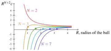
Figure 5. Values of $c$ for $N=2,\dotsc,7$ as a function of $R$. The dot indicates the $R$ such that $2+\lambda_{2}(B_{R})=2^{*}$.

Therefore, as we expected, the numerical experiments indicate that the bifurcation at $p=2+\lambda_{2}$ yields non-radial solutions with energy less than the energy of the trivial solution $1$.

Of course, a bifurcation from the trivial solution $u=1$ is not the only mechanism that can justify the birth of a branch of ground state solutions. Remember that for values of $p$ close to $2$, there is uniqueness of the positive solution and it seems unlikely that a new branch starts from a degenerate ground state at some $p_{0}<2+\lambda_{2}(B_{R})$. Whereas we cannot exclude that situation a priori, we give a numerical evidence that excludes this issue by implementing the mountain pass algorithm [18, 68, 69]. For any tested values $R>0$ and $p<2+\lambda_{2}$, the algorithm finds the constant solution $1$. For our choices of $R>0$ and $p>2+\lambda_{2}$, the algorithm always finds a positive non-radial solution with energy less than the energy of $u=1$ (as it it should be from the results of O. Lopes [40]). We display the outcome of the mountain pass algorithm on Figure 6 (resp. 7) and Table 1 for $N=2$, $p=\lceil 2+\lambda_{2}\rceil$ and $R=1$ (resp. $R=3$). Observe also that the computed solutions look foliated Schwarz symmetric as they should be [63, 66].

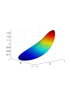
Figure 6. Non radially symmetric least energy solution on $B_{1}\subseteq\mathbb{R}^{2}$.

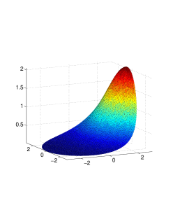
Figure 7. Non radially symmetric least energy solution on $B_{3}\subseteq\mathbb{R}^{2}$.

$R$	$2+\lambda_{2}$		$p$	$\min u$		$\max u$		${{\mathcal{E}}}(u)$		${{\mathcal{E}}}(1)$		$\mathopen{\|}\nabla{{\mathcal{E}}}(u)\mathclose{\|}$
1	5.	39	6	0.	62	1.	36	1.	024	1.	047	1.	6 $\cdot 10^{-9}$
3	2.	38	3	0.	03	2.	05	2.	800	4.	71	1.	6 $\cdot 10^{-12}$

Table 1. Characteristics of non-symmetric ground state $u$ on $B_{R}\subseteq\mathbb{R}^{2}$.

Owing to this foliated Schwarz symmetry, one can also numerically explore the behavior of ground states in $B_{R}\subseteq\mathbb{R}^{N}$ for $N\geqslant 2$. Indeed, we can assume that ground state solutions only depend on

$$(x_{1},\rho):=\bigl{(}x_{1},\sqrt{x_{2}^{2}+\cdots+x_{N}^{2}}\bigr{)}\in\bigl{\{}(x_{1},\rho)\in\mathbb{R}\times\mathbb{R}\bigm{|}x_{1}^{2}+\rho^{2}<R,\ \rho>0\bigr{\}}.$$

Let $(u_{p})_{2<p<2^{*}}$ be a family of ground state solutions. Since $u=1$ is a competitor in the Nehari manifold ${{\mathcal{N}}}_{1,p}$, we have

$${{\mathcal{E}}}_{1,p}(u_{p})=(\tfrac{1}{2}-\tfrac{1}{p})\mathopen{\|}u_{p}\mathclose{\|}_{H^{1}}^{2}\leqslant{{\mathcal{E}}}_{1,p}(1)=(\tfrac{1}{2}-\tfrac{1}{p})\mathopen{\|}1\mathclose{\|}_{H^{1}}^{2}$$

and obviously this implies that ground state solutions are bounded for all $p\in\mathopen{]}2,2^{*}\mathclose{[}$. The graphs in Figures 8 and 9 support the fact that the ground state solution form a continuum bifurcating from $(2+\lambda_{2},1)$.

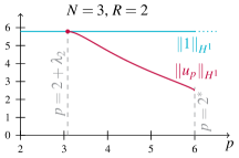
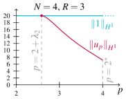
Figure 8. Norm of the ground state $u_{p}$ of ($\mathcal{P}_{1,p}$) on $B_{R}\subseteq\mathbb{R}^{N}$.

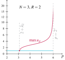
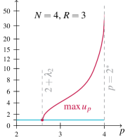
Figure 9. Maximum value of the ground state $u_{p}$ of ($\mathcal{P}_{1,p}$) on $B_{R}\subseteq\mathbb{R}^{N}$.

The graphs of some ground state solutions are given by Figure 10. As expected, when $p\approx 2+\lambda_{2}$, $u_{p}$ looks like $1+\varepsilon\varphi_{2}$ where

$$\varphi{}_{2}(x)=\mathopen{|}x\mathclose{|}^{-\frac{N-2}{2}}J_{N/2}\bigl{(}\sqrt{\lambda_{2}}\mathopen{|}x\mathclose{|}\bigr{)}\,x_{1}$$

is a second eigenfunction of $-\Delta$ that is invariant under rotations in $(x_{2},\dotsc,x_{N})$ centered at $0$. As $p$ approaches $2^{*}$, the solution becomes mostly flat except for a (bounded) bump on the $x_{1}$-axis. We emphasize that for $p=2^{*}$, a least energy solution still exists in $H^{1}$ as established by Wang [65].

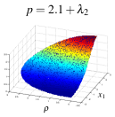
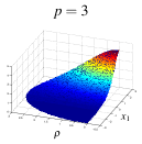
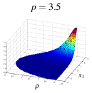
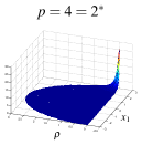
Figure 10. Graphs of ground states on $B_{3}\subseteq\mathbb{R}^{4}$.

These numerical investigations motivate the following conjecture.

Conjecture 6.1.

Let $N\geqslant 2$, $p\in\mathopen{]}2,2^{*}\mathclose{[}$ and $\Omega=B_{R}$.

1. The constant $u=1$ is the least energy solution to ($\mathcal{P}_{1,p}$) if and only if $p\leqslant 2+\lambda_{2}$. In this case, there are no other positive solutions.

2. For $p>2+\lambda_{2}$, least energy solutions belong to the branch bifurcating from $p=2+\lambda_{2}$.

Assertion (a) is supported by the computation of mountain pass solutions. Assertion (b) is motivated by the numerical evidence that the bifurcation at $(2+\lambda_{2},1)$ is super-critical and the investigation along the branch of least energy solutions.

Note that Figures 8 and 9 suggest that the branch of ground state solutions exists for all $p\in\mathopen{]}2,+\infty\mathclose{[}$. Proving that this is indeed the case would be interesting, see Conjecture 1.2 in the Introduction, and will be the subject of a future project.

6.2. The first radial bifurcation

We display in this subsection some numerical computations illustrating the first bifurcation in the space of radially symmetric functions. One naturally expects that on this first branch, the solutions are least energy radial solutions, namely least energy solutions among radial functions. This bifurcation arises at $(1,2+\lambda^{\text{rad}}_{2})$ where $\lambda^{\text{rad}}_{2}$ is the second radial eigenvalue. The numerics are performed on a ball of radius $R=4$ so that $2+\lambda^{\text{rad}}_{2}<2^{*}$ for $N\in\{2,3,4\}$. We recall that this bifurcation is transcritical, as follows from Theorem 3.5. Using the Mountain Pass Algorithm to approximate the least energy radial solution, one gets (as expected) a decreasing solution to ($\mathcal{P}_{1,p}$) different from $1$ for $p\lesssim 2+\lambda^{\text{rad}}_{2}$, as stated by Theorem 3.5. This solution is drawn on the left of Figure 11 and its characteristics are given in Table 2. Using a shooting method, a second positive decreasing solution $u_{2}$ is found. It is pictured on the right of Figure 11 and some characteristics are given in Table 2. It has higher energy that both the previous decreasing solution and $u=1$.

Figure 11. Profile of non constant radial solutions ($p=1.95+\lambda^{\text{rad}}_{2}$).

$$\begin{array}[]{c c r@{.}l|r@{.}l r@{.}l r@{.}l|r@{.}l r@{.}l r@{.}l}N&{2+\lambda^{\text{rad}}_{2}}&\lx@intercol\hfil{{\mathcal{E}}}(1)\hfil\lx@intercol\vrule\lx@intercol&\lx@intercol\hfil\min u_{1}\hfil\lx@intercol&\lx@intercol\hfil\max u_{1}\hfil\lx@intercol&\lx@intercol\hfil{{\mathcal{E}}}(u_{1})\hfil\lx@intercol\vrule\lx@intercol&\lx@intercol\hfil\min u_{2}\hfil\lx@intercol&\lx@intercol\hfil\max u_{2}\hfil\lx@intercol&\lx@intercol\hfil{{\mathcal{E}}}(u_{2})\hfil\lx@intercol\\ \hline\cr 2&2.92&7&604&0&447&2&05&7&45&0&915&1&202&7&606\\ 3&3.26&50&576&0&130&4&05&34&85&0&979&1&095&50&578\\ 4&3.65&280&581&0&016&13&3&66&39&0&999&1&00003&280&581\\ \hline\cr\end{array}$$

Table 2. Characteristics of radial solutions ($p=1.95+\lambda^{\text{rad}}_{2}$, $R=4$).

For $p\in\mathopen{]}2+\lambda^{\text{rad}}_{2},2^{*}\mathclose{[}$, the Mountain Pass Algorithm finds two radial solutions $u_{1}$ and $u_{2}$ to problem ($\mathcal{P}_{1,p}$) depending on the starting point. As an illustration, for $p=2.1+\lambda^{\text{rad}}_{2}$, these solutions are depicted in Figure 12 and their characteristics are given in Table 3. The accuracy is relatively good since $\mathopen{\|}\nabla{{\mathcal{E}}}(u_{i})\mathclose{\|}<10^{-8}$ for $i=1,2$. In agreement with the results of Section 3, they are positive and possess a single intersection with $1$. Moreover, one solution is increasing along the radius and the other one is decreasing.

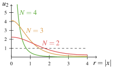
Figure 12. Profile of non constant radial solutions ($p=2.1+\lambda^{\text{rad}}_{2}$).

$$\begin{array}[]{c c r@{.}l|r@{.}l r@{.}l r@{.}l|r@{.}l r@{.}l r@{.}l}N&{2+\lambda^{\text{rad}}_{2}}&\lx@intercol\hfil{{\mathcal{E}}}(1)\hfil\lx@intercol\vrule\lx@intercol&\lx@intercol\hfil\min u_{1}\hfil\lx@intercol&\lx@intercol\hfil\max u_{1}\hfil\lx@intercol&\lx@intercol\hfil{{\mathcal{E}}}(u_{1})\hfil\lx@intercol\vrule\lx@intercol&\lx@intercol\hfil\min u_{2}\hfil\lx@intercol&\lx@intercol\hfil\max u_{2}\hfil\lx@intercol&\lx@intercol\hfil{{\mathcal{E}}}(u_{2})\hfil\lx@intercol\\ \hline\cr 2&2.92&8&48&0&76&1&09&8&47&0&261&2&25&7&39\\ 3&3.26&54&30&0&85&1&03&54&29&0&092&4&12&30&74\\ 4&3.65&294&63&0&90&1&01&294&62&0&008&17&25&49&61\\ \hline\cr\end{array}$$

Table 3. Characteristics of radial solutions ($p=2.1+\lambda^{\text{rad}}_{2}$, $R=4$).

The bifurcation diagram in Figure 13 explains how the above solutions are related: they all belong to the continuum bifurcating from $2+\lambda^{\text{rad}}_{2}$. The increasing solutions on the left of Figure 12 belong to the branch starting to the right of $2+\lambda^{\text{rad}}_{2}$. They have lower energy than $1$ but not the lowest energy. Their radial Morse index, denoted $\operatorname{MI_{rad}}$, is $1$ (they are local minimizers of ${{\mathcal{E}}}_{1,p}$ on the Nehari manifold in $H^{1}_{\text{rad}}$). These solutions still exist in the supercritical range. The decreasing solutions on Figure 11 and on the left of Figure 12 all belong to the branch emanating to the left of $2+\lambda^{\text{rad}}_{2}$. Before the turning point, they have a radial Morse index of $2$ and have higher energy than $1$ (see Figure 14). After the turning point, their radial Morse index is $1$ and, as displayed in Figure 14, they become radial ground states for slightly greater $p$.

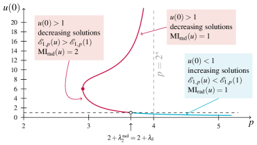
Figure 13. Radial bifurcation branch from $2+\lambda^{\text{rad}}_{2}$ for $N=4$ and $R=4$.

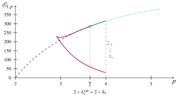
Figure 14. Energy along the radial branches emanating from $2+\lambda^{\text{rad}}_{2}$ for $N=4$ and $R=4$.

The above figures suggest that positive increasing solutions are unique. Increasing solutions must clearly start with $u(0)\in\mathopen{]}0,1\mathclose{[}$. As an additional evidence supporting uniqueness, we have drawn on Figure 15 the time maps

$$u_{0}\mapsto T_{N,p}(u_{0}),$$

where $T_{N,p}(u_{0})$ is the smaller positive number such that $u^{\prime}\bigl{(}T_{N,p}(u_{0})\bigr{)}=0$ with $u$ being the solution to (3.13) such that $u(0)=u_{0}$. These graphs clearly show that $T_{N,p}:\mathopen{]}0,1\mathclose{[}\to\mathbb{R}$ is decreasing and so the equation $T_{n,p}(u_{0})=R$ has at most a solution. Therefore uniqueness holds.

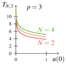
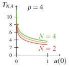
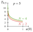
Figure 15. Time maps for increasing solutions for $N\in\{2,3,4\}$.

The preceding considerations naturally lead to some additional conjectures.

Conjecture 6.2.

Let $N\geqslant 2$ and $\Omega=B_{R}$.

1. For any $p>2+\lambda^{\text{rad}}_{2}/\lambda$, there exists a unique positive radial increasing (w.r.t. $\mathopen{|}x\mathclose{|}$) solution to ($\mathcal{P}_{\lambda,p}$) which belongs to the right bifurcation branch coming from $p=2+\lambda^{\text{rad}}_{2}/\lambda$.

2. If $2+\lambda^{\text{rad}}_{2}/\lambda\leqslant 2^{*}$, the least energy radial solutions belong to the radial bifurcation branches coming from $p=2+\lambda^{\text{rad}}_{2}/\lambda$ when $2+\lambda^{\text{rad}}_{2}/\lambda<p<2^{*}$ and, moreover, they are decreasing functions of $\mathopen{|}x\mathclose{|}$;

3. There exists a turning point $\bar{p}<2+\lambda^{\text{rad}}_{2}/\lambda$, such that the solution is degenerate at $\bar{p}$ and there exists two decreasing radial solutions for $\bar{p}<p<2+\lambda^{\text{rad}}_{2}/\lambda$. Moreover the least energy radial solution becomes non constant at some $p_{c}\in\mathopen{[}\bar{p},2+\lambda^{\text{rad}}_{2}/\lambda\mathclose{[}$.

4. If $2+\lambda^{\text{rad}}_{2}/\lambda>2^{*}$, any radial positive ground state solution to ($\mathcal{P}_{\lambda,p}$), $p\in\mathopen{]}2,2^{*}\mathclose{]}$, is the constant function $\lambda^{1/(p-2)}$.

The non degeneracy and uniqueness of the radial increasing solution is proved for large $p$ in [10] so that (a) holds true at least asymptotically as $p\to\infty$. The proof relies on a careful blow up argument which crucially uses the identification of a limit problem for $p\to\infty$.

6.3. Further conjectures and open questions

As proved previously, all branches $B_{i}^{-}$ in the set of , starting to the right of $p=2+\lambda^{\text{rad}}_{i}(B_{R})$, exist for all $p\in\mathopen{]}2+\lambda^{\text{rad}}_{i},+\infty\mathclose{[}$. A natural question is what happens to the radial branch $B_{i}^{+}$ starting to the left of $p=2+\lambda^{\text{rad}}_{i}(B_{R})$. Figures 1, 13 and 16 picture the numerical computation of such branches. They make clear that when $2+\lambda^{\text{rad}}_{i}<2^{*}$, the branch $B_{i}^{+}$ — which was shown to exist for all $p\in\mathopen{[}2+\lambda^{\text{rad}}_{i}-\delta_{i},2^{*}\mathclose{[}$ for some $\delta_{i}>0$ — blows up when $p\to 2^{*}$. The following conjecture is therefore natural.

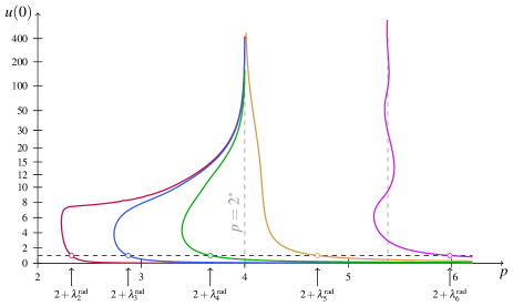
Figure 16. Some radial bifurcation branches from $1$ ($N=4$, $R=9$). The vertical axis is linear up to $10$ and then smoothly switches to a logarithmic scale.

Conjecture 6.3.

Assume that $2+\lambda^{\text{rad}}_{i}<2^{*}$, $i\geqslant 2$, and let $(u_{p})_{2+\lambda^{\text{rad}}_{i}<p<2^{*}}$ be a family of positive radial solutions of type $i_{+}$. When $p\to 2^{*}$, $\mathopen{|}u_{p}\mathclose{|}_{\infty}\to+\infty$ and the solution bifurcates from infinity. In particular, we have

$$\frac{1}{\mathopen{|}u_{p}\mathclose{|}_{\infty}}u_{p}\bigl{(}\mathopen{|}u_{p}\mathclose{|}_{\infty}^{1-p/2}x\bigr{)}\to\Bigl{(}\frac{N(N-2)}{N(N-2)+\mathopen{|}x\mathclose{|}^{2}}\Bigr{)}^{(N-2)/2}$$

uniformly on compact sets.

The fact that all branches $B^{+}_{i}$ starting from $2+\lambda^{\text{rad}}_{i}<2^{*}$ blow up (as indicated by Figure 16) also implies that, if $2+\lambda^{\text{rad}}_{n+1}<2^{*}$, then Problem ($\mathcal{P}_{\lambda,p}$) possesses $n$ positive solutions (distinguished by the nodal properties of $u-1$) whenever $p$ is slightly subcritical. These solution concentrate at $0$ when $p\xrightarrow{<}2^{*}$. The existence of one concentrating solution for slightly subcritical problems was established by O. Rey and J. Wei. In dimension three [60], it concentrates at an interior point while, in dimensions four or greater and for non-convex domains $\Omega$ [61], it concentrates on the least curved part of the boundary $\partial\Omega$. What Figure 16 suggests is that there should actually exist a bubble tower at an interior point (as was shown for the Dirichlet case [23])

The behavior of the branch $B_{i}^{+}$ is more tricky when $2+\lambda^{\text{rad}}_{i}>2^{*}$. We will first focus on the case $i=2$. The shape of the branch depends how small the radius $R$ is but also on the dimension $N$. On Figure 17, the thick line is the branch bifurcating from $(2+\lambda^{\text{rad}}_{2},1)$ and the thin line is another continuum of positive radially decreasing solutions of type $2_{+}$. These graphs suggest that, when $N\in\{4,5,6\}$, no matter how large $2+\lambda^{\text{rad}}_{2}>2^{*}$ is, the left branch starting from $(2+\lambda^{\text{rad}}_{2},1)$ always goes below $2^{*}$, then makes a U-turn and blows up in $L^{\infty}$ as $p\to 2^{*}$. Thus this branch always crosses $p=2^{*}$, which implies the existence of a radially decreasing solution for the critical exponent in accordance with the result of Adimurthi & S. L. Yadava [2]. In this case, for $p\leqslant 2^{*}$, the behavior of the energy along the branch behaves as depicted in Figures 13–14: after the turning point, the radial Morse index changes from $2$ to $1$ and, for $p$ close enough to $2^{*}$, the branch has lower energy than $1$. These numerical computations thus suggest that, in this case, the solution $1$ stops being the radial ground state before $2^{*}$ and this is not due to a sub-critical bifurcation from $1$ but most likely to a bifurcation from infinity (this is part of the assertion (c) in Conjecture 6.2). For $N=3$ or $N\geqslant 7$, Figure 17 shows that when $R$ becomes small, the branch emanating from $(2+\lambda^{\text{rad}}_{2},1)$ does not cross $p=2^{*}$. On the graphs, there is another branch of positive solutions of type $2_{+}$ coming from infinity but this branch must disappear for smaller $R$ because positive solutions are necessarily constant for a sufficiently small radius [2, 3].

Figure 16 also indicates is that, for $R$ large enough, the branch $B_{i}^{+}$ emanating from the first $2+\lambda^{\text{rad}}_{i}$ greater than $2^{*}$ is asymptotic to $2^{*}$. Along that branch, the solutions concentrate at the origin as $p\to 2^{*}$. Proving that this behavior indeed takes place would be a nice complement to results showing the existence of solutions concentrating on the boundary of the domain as $p\xrightarrow{>}2^{*}$ [25, 24]. In addition (as again illustrated by Figure 17), notice that the branches bifurcating from higher $2+\lambda^{\text{rad}}_{i}$ oscillate around some blow up value $p$. This behavior was proved by Miyamoto [48] for ($\mathcal{P}_{\lambda,p}$) but when looking to the bifurcation diagram w.r.t. the parameter $\lambda$. It would be interesting to perform a similar analysis w.r.t. the parameter $p$ and analyze the curves in the $(\lambda,p)$-plane for which entire singular solutions exist (which give the values of the asymptotes of the branches of solutions).

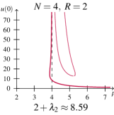
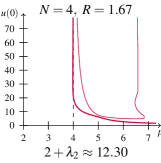
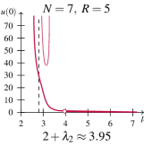
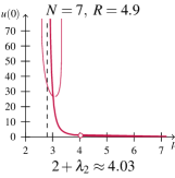
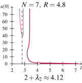
Figure 17. Branch emanating from $2+\lambda^{\text{rad}}_{2}>2^{*}$.

6.4. Evidence of concentration for the singular perturbation problem ($\mathcal{P}_{\varepsilon}$)

In this section, we compute solutions to problem ($\mathcal{P}_{\varepsilon}$) when $\varepsilon$ is small. The bifurcation diagram for $N=3$, $R=4$, $f(u)=\mathopen{|}u\mathclose{|}\,u$ is drawn in Figure 18. Note that, for this $f$, the values of $\varepsilon$ where bifurcation occurs (see (4.1)) are $\varepsilon_{2}\approx 0.7924$, $\varepsilon_{3}\approx 0.2681$, $\varepsilon_{4}\approx 0.1346$, $\varepsilon_{5}\approx 0.0809$, $\varepsilon_{6}\approx 0.0540$, $\varepsilon_{7}\approx 0.0386$,… Figure 19 displays solutions for $\varepsilon=0.05$ on the branches $C^{\pm}_{i}$, $i=2,\dotsc,6$, and shows that the “bumps” cluster around the boundary. Further evidence that the oscillations of the radial solutions of type $i_{+}$ ($i\geqslant 3$) and $i_{-}$ ($i\geqslant 2$) accumulate near the boundary as $\varepsilon\to 0$ is given by Fig. 20 where solutions on the branches $C^{\pm}_{4}$ are drawn. As a consequence, the bifurcating branches from $(\varepsilon_{i},1)$ provide an easy way to construct clustered layer solutions [44]. Since the cubic nonlinearity is subcritical in dimension $3$, the solutions of type $i_{+}$ develop a (bounded) peak at the origin as $\varepsilon\to 0$, the profile being asymptotically that of the rescaled ground state solution in $\mathbb{R}^{3}$.

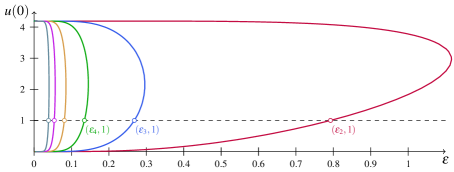
Figure 18. Some radial bifurcation branches emanating from $(\varepsilon_{i},1)$ ($N=3$, $p=3$, $R=4$).

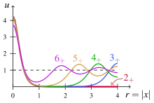
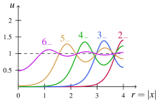
Figure 19. Non constant radial solutions ($N=3$, $p=3$, $R=4$, $\varepsilon=0.05$).

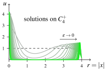
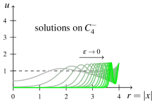
Figure 20. Profile of the solutions along the branch emanating from $\varepsilon_{4}$ ($N=3$, $p=3$, $R=4$).

We now examine more complex nonlinearities $f$ which possess fixpoints in the interval $\mathopen{]}0,1\mathclose{[}$ i.e., Problem ($\mathcal{P}_{\varepsilon}$) possesses more constant solutions than $0$ and $1$. Such fix point will generate an additional homoclinic (asymptotic to this point) for the conservative limit equation $-v^{\prime\prime}+v=f(v)$ which will trap the continuum emanating from $1$ preventing it from reaching the homoclinic asymptotic to $0$ as for the pure power nonlinearity.

More specifically, we consider a function $f_{1}$ such that $u\mapsto F_{1}(u)-u^{2}/2$ (where $F_{1}(u)=\int_{0}^{u}f_{1}$) possesses a single (necessarily degenerate) critical point in $\mathopen{]}0,1\mathclose{[}$ and $f_{2}$ such that $u\mapsto F_{1}(u)-u^{2}/2$ has a local minimum $u^{*}_{1}$ and a local maximum $u^{*}_{2}$ in $\mathopen{]}0,1\mathclose{[}$. These functions are pictured on Fig. 21.

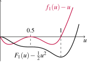
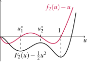
Figure 21. Nonlinearities $f_{i}$, $i=1,2$.

The nonlinearities $f_{1}$ and $f_{2}$ are chosen in such a way that the bifurcations from $1$ occur for the same $\varepsilon_{i}$, $i\geqslant 2$, as for the above pure power ($p=3$).

For both nonlinearities, Figs. 22–24 show that the solutions bifurcating from $1$ behave similarly to those of the pure power case except that their bumps resemble to the homoclinic starting from $0.5$ or $u^{*}_{2}$. Note that, for $f=f_{1}$, the speed of concentration of the bumps is likely to be of order $\varepsilon^{\alpha}$ for some $\alpha>0$ due to the degeneracy of the critical point $0.5$ which implies that the associated homoclinic decays like a power.

For $f=f_{1}$, there are additional solutions $u$ with $u(0)\in\mathopen{]}0,0.5\mathclose{[}$. These solutions seem to come in pairs: for $\varepsilon>0$ small enough, there are two solutions of type $i_{-}$, one starting close to the homoclinic asymtotic to $0$ and another one increasing to $0.5$ and then resembling the homoclinic asymtotic to $0.5$ before oscillating around $1$ (see the right graph of Fig. 23).

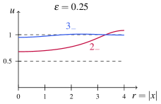
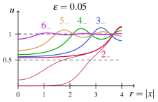
Figure 22. Non constant radial solutions ($N=3$, $f=f_{1}$, $R=4$, $\varepsilon\to 0$).

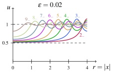
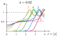
Figure 23. Non constant radial solutions ($N=3$, $f=f_{1}$, $R=4$, $\varepsilon=0.02$).

For $f=f_{2}$, the additional numerically computed solutions oscillate around the second local minimum $u^{*}_{1}$ of $u\mapsto F_{2}(u)-\frac{1}{2}u^{2}$ (see Fig. 24). For these solutions, the classification in types $i_{\pm}$ has to be adapted to count the number of zeros of $u-u^{*}_{1}$ with the subscript $\pm$ being the sign of $u(0)-u^{*}_{1}$. Assuming that $f^{\prime}(u^{*}_{1})>1$ (i.e., that the minimum $u^{*}_{1}$ is non-degenerate) and following similar arguments to those developed above, one can prove a multiplicity result such as Corollary 4.4. In this case however, both solutions of type $i_{-}$ and $i_{+}$ will keep existing no matter how small $\varepsilon>0$ is, so, when $\varepsilon<(f^{\prime}(u^{*}_{1})-1)/\lambda^{\text{rad}}_{n+1}$, one will actually have at least $2n$ solutions to Problem ($\mathcal{P}_{\varepsilon}$), one for each type $i_{\pm}$, $2\leqslant i\leqslant n+1$.

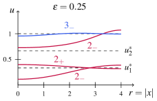
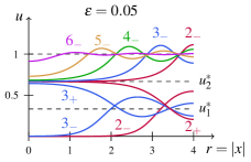
Figure 24. Non constant radial solutions ($N=3$, $f=f_{2}$, $R=4$, $\varepsilon\to 0$).

References

- [1] A. Malchiodi A. Ambrosetti. Perturbation methods and semilinear elliptic problems on . Progress in Mathematics, 240. Birkhauser Verlag, Basel, 2006.
- [2] Adimurthi and S. L. Yadava. Existence and nonexistence of positive radial solutions of Neumann problems with critical Sobolev exponents. Arch. Rational Mech. Anal., 115(3):275–296, 1991.
- [3] Adimurthi and S. L. Yadava. Nonexistence of positive radial solutions of a quasilinear Neumann problem with a critical Sobolev exponent. Arch. Rational Mech. Anal., 139:239–253, 1997.
- [4] Amandine Aftalion and Filomena Pacella. Qualitative properties of nodal solutions of semilinear elliptic equations in radially symmetric domains. C. R. Math. Acad. Sci. Paris, 339(5):339–344, 2004.
- [5] Antonio Ambrosetti, Andrea Malchiodi, and Wei-Ming Ni. Singularly perturbed elliptic equations with symmetry: existence of solutions concentrating on spheres. II. Indiana Univ. Math. J., 53(2):297–329, 2004.
- [6] Antonio Ambrosetti and Giovanni Prodi. A primer of nonlinear analysis, volume 34 of Cambridge Studies in Advanced Mathematics. Cambridge University Press, Cambridge, 1995. Corrected reprint of the 1993 original.
- [7] Thomas Bartsch, Mónica Clapp, Massimo Grossi, and Filomena Pacella. Asymptotically radial solutions in expanding annular domains. Math. Ann., 352(2):485–515, 2012.
- [8] Vivina Barutello, Simone Secchi, and Enrico Serra. A note on the radial solutions for the supercritical Hénon equation. J. Math. Anal. Appl., 341(1):720–728, 2008.
- [9] Reinhold Böhme. Die lösung der verzweigungsgleichungen für nichtlineare eigenwertprobleme. Math. Z., 127:105–126, 1972. (German).
- [10] D. Bonheure, M. Grossi, and B. Noris. Multi-layer radial solutions for a supercritical Neumann problem. arXiv:1508.01619, 2015.
- [11] Denis Bonheure, Vincent Bouchez, and Christopher Grumiau. Asymptotics and symmetries of ground-state and least energy nodal solutions for boundary-value problems with slowly growing superlinearities. Differential Integral Equations, 22(9-10):1047–1074, 2009.
- [12] Denis Bonheure, Benedetta Noris, and Tobias Weth. Increasing radial solutions for Neumann problems without growth restrictions. Ann. Inst. H. Poincaré Anal. Non Linéaire, 29(4):573–588, 2012.
- [13] Denis Bonheure and Enrico Serra. Multiple positive radial solutions on annuli for nonlinear Neumann problems with large growth. NoDEA, Nonlinear Differ. Equ. Appl., 18(2):217–235, 2011.
- [14] Haïm Brézis and Louis Nirenberg. Positive solutions of nonlinear elliptic equations involving critical Sobolev exponents. Comm. Pure Appl. Math., 36(4):437–477, 1983.
- [15] Haim Brezis and Walter A. Strauss. Semi-linear second-order elliptic equations in . J. Math. Soc. Japan, 24(4):565–590, 1973.
- [16] Robert F. Brown. A topological introduction to nonlinear analysis. Birkhäuser Boston Inc., Boston, MA, 1993.
- [17] C. Budd, M. Knapp, and L. Peletier. Asymptotic behaviour of solutions of elliptic equations with critical exponent and Neumann boundary conditions. Proc. Roy. Soc. Edinburgh, 117:225–250, 1991.
- [18] Yung Sze Choi and P. Joseph McKenna. A mountain pass method for the numerical solution of semilinear elliptic problems. Nonlinear Anal., 20(4):417–437, 1993.
- [19] Vittorio Coti Zelati and Maria J. Esteban. Symmetry breaking and multiple solutions for a Neumann problem in an exterior domain. Proc. R. Soc. Edinb., Sect. A, 116(3-4):327–339, 1990.
- [20] Michael G. Crandall and Paul H. Rabinowitz. Bifurcation from simple eigenvalues. Journal of Functional Analysis, 8(2):321–340, October 1971.
- [21] Lucio Damascelli, Massimo Grossi, and Filomena Pacella. Qualitative properties of positive solutions of semilinear elliptic equations in symmetric domains via the maximum principle. Ann. Inst. H. Poincaré Anal. Non Linéaire, 16(5):631–652, 1999.
- [22] Teresa D’Aprile and Angela Pistoia. On the existence of some new positive interior spike solutions to a semilinear Neumann problem. J. Differential Equations, 248(3):556–573, 2010.
- [23] Manuel Del Pino, Jean Dolbeault, and Monica Musso. “Bubble-tower” radial solutions in the slightly supercritical Brezis-Nirenberg problem. J. Differential Equations, 193(2):280–306, 2003.
- [24] Manuel del Pino, Fethi Mahmoudi, and Monica Musso. Bubbling on boundary submanifolds for the Lin-Ni-Takagi problem at higher critical exponents. J. Eur. Math. Soc. (JEMS), 16(8):1687–1748, 2014.
- [25] Manuel del Pino, Monica Musso, and Angela Pistoia. Super-critical boundary bubbling in a semilinear Neumann problem. Ann. Inst. Henri Poincaré Anal., 22-1, 2005.
- [26] Maria J. Esteban. Rupture de symétrie pour des problèmes de Neumann sur-linéaires dans des ouverts extérieurs. C. R. Acad. Sci. Paris Sér. I Math., 308(10):281–286, 1989.
- [27] Maria J. Esteban. Nonsymmetric ground states of symmetric variational problems. Commun. Pure Appl. Math., 44(2):259–274, 1991.
- [28] Basilis Gidas, Wei-Ming Ni, and Louis Nirenberg. Symmetry and related properties via the maximum principle. Comm. Math. Phys., 68(3):209–243, 1979.
- [29] Basilis Gidas and Joel Spruck. A priori bounds for positive solutions of nonlinear elliptic equations. Comm. Partial Differential Equations, 6(8):883–901, 1981.
- [30] A. Gierer and H. Meinhardt. A theory of biological pattern formation. Kybernetik, 12:30–39, 1972.
- [31] Massimo Grossi and Benedetta Noris. Positive constrained minimizers for supercritical problems in the ball. Proc. Amer. Math. Soc., 140(6):2141–2154, 2012.
- [32] Massimo Grossi, Angela Pistoia, and Juncheng Wei. Existence of multipeak solutions for a semilinear Neumann problem via nonsmooth critical point theory. Calc. Var. Partial Differential Equations, 11(2):143–175, 2000.
- [33] Christopher Grumiau and Christophe Troestler. Oddness of least energy nodal solutions on radial domains. Elec. Journal of diff. equations, Conference 18:23–31, 2010.
- [34] Yoshitsugu Kabeya and Wei-Ming Ni. Stationary Keller-Segel model with the linear sensitivity. Sūrikaisekikenkyūsho Kōkyūroku, (1025):44–65, 1998. Variational problems and related topics (Japanese) (Kyoto, 1997).
- [35] E.F. Keller and L.A. Segel. Initiation of slime mold aggregation viewed as an instability. J. Theor. Biol., 26:399–415, 1970.
- [36] Philip Korman. A global solution curve for a class of semilinear equations. In Proceedings of the Third Mississippi State Conference on Difference Equations and Computational Simulations (Mississippi State, MS, 1997), volume 1 of Electron. J. Differ. Equ. Conf., pages 119–127 (electronic). Southwest Texas State Univ., San Marcos, TX, 1998.
- [37] M. A. Krasnosel’skii. Topological methods in the theory of nonlinear integral equations. Translated by A. H. Armstrong; translation edited by J. Burlak. A Pergamon Press Book. The Macmillan Co., New York, 1964.
- [38] C. S. Lin and W. M. Ni. On the diffusion coefficient of a semilinear Neumann problem. Springer Lecture Notes, 340:160–174, 1986.
- [39] C.-S. Lin, W.-M. Ni, and I. Takagi. Large amplitude stationary solutions to a chemotaxis system. J. Diff. Eqns., 72:1–27, 1988.
- [40] Orlando Lopes. Radial and nonradial minimizers for some radially symmetric functionals. Electron. J. Differ. Equ., 3, 1996.
- [41] Lee Lorch and Martin E. Muldoon. Monotonic sequences related to zeros of bessel functions. Numerical Algorithms, 49(1–4):221–233, December 2008.
- [42] Fethi Mahmoudi and Andrea Malchiodi. Concentration on minimal submanifolds for a singularly perturbed Neumann problem. Adv. Math., 209(2):460–525, 2007.
- [43] A. Malchiodi. Concentration at curves for a singularly perturbed Neumann problem in three-dimensional domains. Geom. Funct. Anal., 15(6):1162–1222, 2005.
- [44] A. Malchiodi, Wei-Ming Ni, and Juncheng Wei. Multiple clustered layer solutions for semilinear Neumann problems on a ball. Ann. Inst. H. Poincaré Anal. Non Linéaire, 22(2):143–163, 2005.
- [45] Andrea Malchiodi and Marcelo Montenegro. Multidimensional boundary layers for a singularly perturbed Neumann problem. Duke Math. J., 124(1):105–143, 2004.
- [46] Antonio Marino. La biforcazione nel caso variazionale. Confer. Sem. Mat. Univ. Bari, (132):14, 1973.
- [47] Jean Mawhin and Michel Willem. Critical Point Theory and Hamiltonien Systems. Springer, New York, Heidelberg, London, Paris, Tokyo, 1989.
- [48] Y. Miyamoto. Structure of the positive radial solutions for the supercritical Neumann problem in a ball. Journal of Mathematical Sciences, the University of Tokyo, 22:685–739, 2015.
- [49] Wei Ming Ni. On the positive radial solutions of some semilinear elliptic equations on . Appl. Math. Optim., 9(4):373–380, 1983.
- [50] Wei-Ming Ni. Diffusion, cross-diffusion, and their spike-layer steady states. Notices Amer. Math. Soc., 45(1):9–18, 1998.
- [51] Wei-Ming Ni and Roger D. Nussbaum. Uniqueness and nonuniqueness for positive radial solutions of . Commun. Pure Appl. Math., 38:67–108, 1985.
- [52] Wei-Ming Ni and Izumi Takagi. On the Neumann problem for some semilinear elliptic equations and systems of activator-inhibitor type. Transactions of the american Mathematical society, 297(1):351–368, 1986.
- [53] Wei-Ming Ni and Izumi Takagi. On the shape of least-energy solutions to a semilinear Neumann problem. Comm. Pure Appl. Math., 44(7):819–851, 1991.
- [54] Wei-Ming Ni and Izumi Takagi. Locating the peaks of least-energy solutions to a semilinear Neumann problem. Duke Math. J., 70(2):247–281, 1993.
- [55] National Institute of Standards and Technology. Digital library of mathematical functions. http://dlmf.nist.gov/.
- [56] Stanislav I. Pohozaev. On the eigenfunctions of the equation . Dokl. Akad. Nauk SSSR., 165:36–39, 1965.
- [57] Paul H. Rabinowitz. A bifurcation theorem for potential operators. J. Functional Analysis, 25(4):412–424, 1977.
- [58] Paul H. Rabinowitz. Global Aspects of Bifurcation. Sém. Math. Sup., 91:63–112, 1985.
- [59] Mythily Ramaswamy and P. N. Srikanth. Symmetry breaking for a class of semilinear elliptic problems. Trans. Amer. Math. Soc., 304(2):839–845, 1987.
- [60] Olivier Rey and Juncheng Wei. Blowing up solutions for an elliptic Neumann problem with sub- or supercritical nonlinearity. I. . J. Funct. Anal., 212(2):472–499, 2004.
- [61] Olivier Rey and Juncheng Wei. Blowing up solutions for an elliptic Neumann problem with sub- or supercritical nonlinearity. II. . Ann. Inst. H. Poincaré Anal. Non Linéaire, 22(4):459–484, 2005.
- [62] Enrico Serra and Paolo Tilli. Monotonicity constraints and supercritical Neumann problems. Ann. Inst. Henri Poincaré, Anal. Non Linéaire , 28-1:63–74, 2011.
- [63] Jean Van Schaftingen. Symmetrization and minimax principles. Commun. Contemp. Math., 7(4):463–481, 2005.
- [64] Liping Wang, Juncheng Wei, and Shusen Yan. A Neumann problem with critical exponent in nonconvex domains and Lin-Ni’s conjecture. Trans. Amer. Math. Soc., 362(9):4581–4615, 2010.
- [65] Xu Jia Wang. Neumann problems of semilinear elliptic equations involving critical Sobolev exponents. J. Differential Equations, 93(2):283–310, 1991.
- [66] Tobias Weth. Symmetry of solutions to variational problems for nonlinear elliptic equations via reflection methods. Jahresber. Dtsch. Math.-Ver., 112-3, 2010.
- [67] Li YanYan and Zhang Lei. Liouville-type theorems and harnack-type inequalities for semilinear elliptic equations. Journal d’Analyse Mathématique, 90(1):27–87, 2003.
- [68] Jianxin Zhou and Youngxin Li. A minimax method for finding multiple critical points and its applications to semilinear elliptic pde’s. SIAM Sci.Comp., 23:840–865, 2001.
- [69] Jianxin Zhou and Youngxin Li. Convergence results of a local minimax method for finding multiple critical points. SIAM Sci. Comp., 24:865–885, 2002.