Quantification of Uncertainties in Turbulence Modeling: A Comparison of Physics-Based and Random Matrix Theoretic Approaches

Abstract

Numerical models based on Reynolds-Averaged Navier-Stokes (RANS) equations are widely used in engineering turbulence modeling. However, the RANS predictions have large model-form uncertainties for many complex flows, e.g., those with non-parallel shear layer or strong mean flow curvature. Quantification of these large uncertainties originating from the modeled Reynolds stresses has attracted attention in turbulence modeling community. Recently, a physics-based Bayesian framework for quantifying model-form uncertainties has been proposed with successful applications to several flows. Nonetheless, how to specify proper priors without introducing unwarranted, artificial information remains challenging to the current form of the physics-based approach. Another recently proposed method based on random matrix theory provides the prior distributions with the maximum entropy, which is an alternative for model-form uncertainty quantification in RANS simulations. This method has better mathematical rigorousness and provides the most non-committal prior distributions without introducing artificial constraints. On the other hand, the physics-based approach has the advantages of being more flexible to incorporate available physical insights. In this work, we utilize the random matrix theoretic approach to assess and possibly improve the specification of priors used in the physics-based approach. A comparison of the two approaches is then conducted through a test case using a canonical flow, the flow past periodic hills. The numerical results show that, to achieve maximum entropy in the prior of Reynolds stresses, the perturbations of shape parameters in Barycentric coordinates are normally distributed. Moreover, the perturbations of the turbulence kinetic energy should conform to log-normal distributions. Finally, it sheds light on how large the variance of each physical variable should be compared with each other to achieve the approximate maximum entropy prior. The conclusion can be used as a guidance for specifying proper priors in the physics-based, Bayesian uncertainty quantification framework.

Highlights

1. Compared physics-based and random matrix methods to quantify RANS model uncertainty

2. Demonstrated applications of both methods in channel flow over periodic hills

3. Examined the amount of information introduced in the physics-based approach

4. Discussed implications to modeling turbulence in both near-wall and separated regions

Notations

We summarize the convention of notations below because of the large number of symbols used in this paper. The general conventions are as follows:

1. Upper case letters with brackets (e.g., $[R]$) indicate matrices or tensors; lower case letters with arrows (e.g., $\vec{v}$) indicate vectors; undecorated letters in either upper or lower cases indicate scalars. An exception is the spatial coordinate, which is denoted as $x$ for simplicity but is in fact a $3\times 1$ vector. Tensors (matrices) and vectors are also indicated with index notations, e.g., $R_{ij}$ and $v_{i}$ with $i,j=1,2,3$.

2. Bold letters (e.g., $[\mathbf{R}]$) indicate random variables (including scalars, vectors, and matrices), the non-bold letters (e.g., $[R]$) indicate the corresponding realizations, and underlined letters (e.g., $[\underline{R}]$) indicate the mean.

3. Symbols ${M}_{d}^{+}$, and $\mathbb{M}_{d}^{+0}$ indicate the sets of symmetric positive definite and symmetric positive semi-definite matrices, respectively, of dimension $d\times d$ with the following relation: $\mathbb{M}_{d}^{s}\subset{M}_{d}^{+}\subset\mathbb{M}_{d}^{+0}$.

This work deals with Reynolds stresses, which are rank two tensors. Therefore, it is implied throughout the paper that all random or deterministic matrices have sizes $3\times 3$ with real entries unless noted otherwise. Finally, a list of nomenclature is presented in C.

1 Introduction

Despite the increasing availability of computational resources in the past decades, high-fidelity simulations (e.g., large eddy simulation, direct numerical simulation) are still not affordable for most practical problems. Numerical models based on Reynolds-Averaged Navier–Stokes (RANS) equations are still the dominant tools for the prediction of turbulent flows in industrial and natural processes. However, for many practical flows, e.g., those with strong adverse pressure gradient, non-parallel shear layer, or strong mean flow curvature, the predictions of RANS models have large uncertainties. The uncertainties are mostly attributed to the phenomenological closure models for the Reynolds stresses [1, 2]. Previous efforts in quantifying and reducing model-form uncertainties in RANS simulations have mostly followed parametric approaches, e.g., by perturbing, tuning, or inferring the parameters of the closure models of the Reynolds stress [3, 4, 5].

Recently, the turbulence modeling community has recognized the limitations of the parametric approaches and started investigating non-parametric approaches where uncertainties are directly injected into the Reynolds stresses [2, 6, 7, 8, 9, 10]. In their pioneering work, Iaccarino et al. [6, 8, 9] proposed a physics-based approach, where the Reynolds stress is projected onto six physically meaningful dimensions (its shape, magnitude, and orientation). They further perturbed the Reynolds stresses towards the limiting states in the physically realizable range, based on which the RANS prediction uncertainties are estimated. Building on the work of Iaccarino et al. [6, 8, 9], Xiao et al. [10] modeled the Reynolds stress discrepancy as a zero-mean random field and used a physical-based parameterization to systematically explore the uncertainty space. They further used Bayesian inferences to incorporate observation data to reduce the model-form uncertainty in RANS simulation. While the physics-based method has achieved significant successes, the method in its current form has two major limitations. First, uncertainties are only injected to the shape and magnitude of the Reynolds stresses but not to the orientations, and thus they do not fully explore the uncertainty space. Second, it is challenging to specify prior distributions over these physical variables without introducing artificial constraints. The priors are critical for uncertainty propagation and Bayesian inference, particularly when the amount of data is limited [11]. Xiao et al. [10] specified Gaussian distribution for the perturbations of shape parameters in natural coordinates and log-normal distribution for the turbulence kinetic energy discrepancy. The perturbations in all physical parameters share the same variance field. However, it is not clear if or how much artificial constraints are introduced into the prior with this choice. Moreover, without sufficient physical insight, it is not clear how large the variance of perturbation for each physical variable should be relative to each other.

In information theory, Shannon entropy is an important measure of the information contained in each probability distribution. The distribution best representing the current state is the one with the largest information entropy, which is known as principle of maximum entropy [12]. This principle has been used as a guideline to specify prior distributions in Bayesian framework [13]. Although this theory has been extensively used in information processing problems such as communications and image processing, the application in conjunction with random matrix theory applied to physical systems is only a recent development, which was first proposed and developed by Soize et al. [14, 15]. Built on the theories developed by Soize et al., Xiao et al. [16] proposed a random matrix theoretic (RMT) approach with maximum entropy principle to quantify model-form uncertainties in RANS simulations. The RMT approach is an alternative to the physics-based approach in quantifying model-form uncertainties in RANS simulations. It can provide objective priors for Bayesian inferences that satisfies the given constraints without introducing artificial information.

While the RMT approach has better mathematical rigorousness and provides a proper prior of the Reynolds stress tensors with maximum entropy, it has its own limitations. In particular, since the perturbations are directly introduced to the Reynolds stress itself, it is not straightforward to incorporate physical insights that are available for specific flows into the RMT approach. For example, for the flow in a channel with square cross section, the discrepancies of RANS-predicted Reynolds stress mainly come from the shape of the Reynolds stress tensor, while the predicted turbulence kinetic energy is rather accurate [17]. In this case, the perturbation variances of shape parameters should be specified much larger than that of the turbulence kinetic energy. Nonetheless, this piece of information is difficult to incorporate into the RMT approach. In comparison, the physics-based approach is more flexible and thus may be preferred in engineering applications for both uncertainty quantification and Bayesian inferences. Therefore, the objective of this work is to utilize the RMT approach to assess and improve the specification of priors used in the physics-based approach. To this end, the Reynolds stress samples with maximum entropy distribution obtained in the RMT approach are first projected onto the physically meaningful dimensions. Then, the distributions in the six physical dimensions are used to gauge the priors specified in the physics-based approach. The comparison between the two approaches allows for quantification of the amount of information introduced in the physics-based priors. It also sheds light on the specification of appropriate prior for each physical variable when no further physical knowledge is available.

The rest of the paper is organized as follows. Section 2 introduces the physics-based and RMT approaches for RANS model-form uncertainty quantification. Section 3 uses the flow over periodic hills as an example to perform the comparison between the two approaches. The results are then presented and discussed. Finally, Section 4 concludes the paper.

2 Comparison of Physics Based Approach and RMT Approach

This work examines and compares two approaches, the physics-based approach and the random matrix theoretic approach, for quantifying RANS model-form uncertainties. We first briefly introduce the general background of RANS-based turbulence modeling and the common assumptions of the two approaches before presenting the technical details of the two approaches.

Reynolds averaged Navier–Stokes equations describe the mean quantities (e.g., velocity and pressure) of the turbulent flows. They are obtained by performing time- or ensemble-averaging on the Navier–Stokes equations, which describes the instantaneous flow quantities. The averaging process leads to a covariance term of the instantaneous velocities, which is referred to as Reynolds stresses and needs model closure in RANS simulations. It is the consensus of the turbulence modeling community that the modeling of the Reynolds stresses accounts for majority of the model-form uncertainty in RANS simulations [1]. In the physics based approach proposed by Iaccarino et al.[6, 8] and further extended by Xiao et al. [10, 11], perturbations are directly injected to the RANS-predicted Reynolds stresses. Specifically, the physically meaningful projections of the Reynolds stress, i.e., its magnitude, shape, and orientation are jointly perturbed around their respective mean values obtained in the RANS simulation, and the perturbations are then propagated through RANS solvers to the Quantities of Interests (QoI, e.g., velocities). The obtained ensemble is then used to assess the uncertainties in the RANS predictions. The specific form of perturbation for each variable is a modeling choice made by the user. The scheme ensures realizability (positive semi-definiteness) of the Reynolds stresses. Similar to the physics-based approach, zero-mean perturbations are also injected to the RANS-predicted Reynolds stresses in the RMT approach with realizability guaranteed. In contrast to the physics-based approach, however, in the RMT approach the true Reynolds stress is modeled as random matrices, for which a maximum entropy probabilistic distribution is constructed under the constraint that the mean is the RANS-predicted value. The maximum entropy distribution is then sampled to be obtain the perturbed Reynolds stress fields.

In summary, both the physics-based and the RMT approaches introduce zero-mean perturbations to the RANS predicted Reynolds stresses, which are then propagated to the QoIs to assess RANS prediction uncertainties. They differ in how the perturbations are introduced. The RMT approach introduces perturbations directly in the Reynolds stress tensor and the perturbations conform to a maximum entropy distribution, while the physics-based approach introduces perturbations to the physically meaningful projections of the Reynolds stresses. The details of the two schemes are presented below.

2.1 Physics-Based Approach

Here, we briefly summarize the physics-based model-form uncertainty quantification framework proposed by Xiao et al. [10] and its extension to account for uncertainties in tensor orientation. In the framework, the true Reynolds stress $[\mathbf{R}(x)]$ is modeled as a random tensorial field with the RANS-predicted Reynolds stress $[R(x)]^{rans}$ as prior mean, in which $x$ denotes the spatial coordinate. To inject uncertainties into the physically meaningful projections of Reynolds stress tensor, the following eigen-decomposition is performed for its each realization at any given location $x$:

$$[R]=2k\left(\frac{1}{3}[I]+[A]\right)=2k\left(\frac{1}{3}[I]+[E][\Lambda][E]^{T}\right)$$ (1)

where $k$ is the turbulent kinetic energy indicating the magnitude of $[R]$; $[I]$ is the second order identity tensor; $[A]$ is the anisotropy tensor; $[E]=[\vec{e}_{1},\vec{e}_{2},\vec{e}_{3}]$ and $[\Lambda]=\textrm{diag}[\tilde{\lambda}_{1},\tilde{\lambda}_{2},\tilde{\lambda}_{3}]$ ,where $\tilde{\lambda}_{1}+\tilde{\lambda}_{2}+\tilde{\lambda}_{3}=0$, are the orthonormal eigenvectors and the corresponding eigenvalues of $[A]$, respectively, indicating the orientation and shape of $[R]$. In order to physically interpret the shape of the Reynolds stress and easily impose the realizability constraint, the eigenvalues $\tilde{\lambda}_{1}$, $\tilde{\lambda}_{2}$, and $\tilde{\lambda}_{3}$ are mapped to the Barycentric coordinates $(C_{1},C_{2},C_{3})$ with $C_{1}+C_{2}+C_{3}=1$. The Barycentric coordinates are defined as,

$$C_{1} =\tilde{\lambda}_{1}-\tilde{\lambda}_{2}$$ (2a)

$$C_{2} =2(\tilde{\lambda}_{2}-\tilde{\lambda}_{3})$$ (2b)

$$C_{3} =3\tilde{\lambda}_{3}+1\ .$$ (2c)

As shown in Fig. 1a, the Barycentric coordinates ($C_{1}$, $C_{2}$, $C_{3}$) of a point indicate the portion of areas of three sub-triangles formed by the point and with edge labeled as $C_{1}$, $C_{2}$, and $C_{3}$, in the Barycentric triangle. For example, the ratio of the sub-triangle labeled with $C_{3}$ to the entire triangle is $C_{3}$. A point located on the top vertex corresponds to $C_{3}=1$ while a point located on the bottom edge has $C_{3}$ = 0.

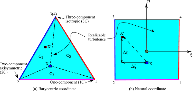
Figure 1: Mapping between the Barycentric coordinate to the natural coordinate, transforming the Barycentric triangle enclosing all physically realizable states [18, 8] to a square through standard finite element shape functions. Details of the mapping can be found in the appendix of ref. [10]. Corresponding edges in the two coordinates are indicated with matching colors.

The Barycentric coordinates have clear physical interpretation, i.e., the dimensionality of the turbulence. All the edges and vertices indicate limiting states of turbulence, which are shown in Fig 1a. The projections of all Reynolds stresses should fall inside the Barycentric triangle to ensure the realizability. To facilitate parameterization, the Barycentric coordinates are further transformed to the natural coordinates $(\xi,\eta)$ with the triangle mapped to the square, as shown in Fig. 1b. Details of the mapping can be found in ref. [10]. Although the tensor orientation ($[E]=[\vec{e}_{1},\vec{e}_{2},\vec{e}_{3}]$) has not been perturbed in ref. [10], it can be done with an appropriate parameterization scheme. The Euler angle with $z$-$x^{\prime}$-$z^{\prime\prime}$ convention [19] is used to parameterize the orientation of the Reynolds stress tensor. That is, first, the local coordinate system $x$-$y$-$z$ of eigenvectors of $[\mathbf{R}]$ initially aligned with the global coordinate system $X$-$Y$-$Z$ rotates about the $z$ axis by angle $\varphi_{1}$. Then, it rotates about the $x$ axis by angle $\varphi_{2}$, and finally rotates about its new $z$ axis by angle $\varphi_{3}$.

In summary, the Reynolds stress tensor field is transformed to six physically meaningful component fields denoted as $\xi,\eta,k,\varphi_{1},\varphi_{2}$, and $\varphi_{3}$, which are all scalar fields. After the mapping, uncertainties are introduced to these quantities by adding discrepancy terms to the corresponding RANS predictions, i.e.,

$$\xi(x) = \ \tilde{\xi}^{rans}(x) +\Delta\xi(x)$$ (3a)

$$\eta(x) = \ \tilde{\eta}^{rans}(x) +\Delta\eta(x)$$ (3b)

$$\log k(x) = \ \log\tilde{k}^{rans}(x) +\Delta\log k(x)$$ (3c)

$$\varphi_{i}(x) = \ \tilde{\varphi_{i}}^{rans}(x) +\Delta\varphi_{i}(x),\ \ i=1,2,3$$ (3d)

where $\Delta\xi(x)$ and $\Delta\eta(x)$ are discrepancies of the Reynolds stress shape parameters $\xi$ and $\eta$, respectively; $\Delta\log k(x)$ is the log-discrepancy of the turbulent kinetic energy; $\Delta\varphi_{i}(x)$ $(i=1,2,3)$ are the discrepancies of three Euler angles. To model the prior of these discrepancy fields with spatial smoothness, we assume that each discrepancy field is normally distributed at any location $x$ and use a Gaussian kernel $K(x,x^{\prime})$ to describe the correlation between any two different locations $x$ and $x^{\prime}$. That is,

$$K(x,x^{\prime})=\sigma(x)\sigma(x^{\prime})\exp\left(-\frac{|x-x^{\prime}|^{2}}{l^{2}}\right)\quad\textrm{where}\;x,x^{\prime}\in\Sigma,$$ (4)

where $\Sigma$ is the spatial domain of the flow field. The variance $\sigma(x)$ is a spatially varying field representing the magnitude of injected uncertainties. The correlation length $l$ also varies spatially based on the local length scale of the mean flow. It can be seen from Eq. 3 that the discrepancy fields for shape parameters ($\xi$, $\eta$) and Euler angles ($\varphi_{i}$) are Gaussian random fields, and the discrepancy field for magnitude parameter $k$ is a log-normal random field. To reduce dimensions of the random fields, Karhunen–Loeve expansions of the random fields are adopted with chosen basis that are eigenfunctions of the kernel [20]. That is, the discrepancies can be represented as follows:

$$\Delta(x)=\sum_{j=1}^{\infty}\omega_{\alpha}\;\phi_{\alpha}(x),$$ (5)

where the coefficients $\omega_{\alpha}$ (denoting $\omega^{\xi}_{\alpha}$, $\omega^{\eta}_{\alpha}$, $\omega^{k}_{\alpha}$, $\omega^{\varphi_{i}}_{\alpha}$ for discrepancy fields $\Delta\xi$, $\Delta\eta$, $\Delta\log k$ and $\Delta\varphi_{i}$, respectively) are independent standard Gaussian random variables. In practice, the infinite series are truncated to $N_{kl}$ terms with $N_{kl}$ depending on the smoothness of the kernel $K$. Therefore, the discrepancy fields in Reynolds stress are parameterized by the coefficients $\omega^{\xi}_{\alpha},\,\omega^{\eta}_{\alpha},\,\omega^{k}_{\alpha},\,\omega^{\varphi_{i}}_{\alpha}$ with $\alpha=1,2,\cdots,N_{kl}$. These Reynolds stress discrepancies are then propagated to the QoI (e.g., velocity) as the model-form uncertainties.

In summary, the uncertainties are injected into the six physically meaningful dimensions of Reynolds stress separately in the physics-based approach. For each dimension, the uncertainties are represented by the Gaussian random fields to ensure the smoothness of the Reynolds stress perturbations (for incompressible flow). The perturbed Reynolds stresses are reconstructed with these six random fields, which are then propagated to the QoI as the quantified model-form uncertainties. Detailed algorithm of the physics-based approach is presented in A.

2.2 Random Matrix Theoretic Approach with Maximum Entropy Principle

Since Reynolds stresses belong to the set $\mathbb{M}_{d}^{+0}$ of symmetric positive definite tensors, where $d=3$, it is natural to describe them directly as random matrices in set $\mathbb{M}_{d}^{+0}$. In the following, we summarize the uncertainty quantification approach based on random matrix theory and maximum entropy principle proposed by Xiao et al. [16]. In this framework, a probabilistic model in matrix set is built to satisfy all the constraints in the context of turbulence modeling. Based on the principle of maximum entropy, the target probability measure $p_{[\text{{\tiny R}}]}:\mathbb{M}_{d}^{+0}\mapsto\mathbb{R}^{+}$ is the most non-committal probability density function (PDF) satisfying all available constraints (e.g., realizability) but without introducing any other unwarranted constraints, where $\mathbb{R}^{+}$ is the set of positive real number.

A two-step approach is used to find such maximum entropy distribution for random Reynolds stress tensors. First, the PDF for a normalized, positive definite random matrix $[\mathbf{G}]$ is obtained, whose mean is the identity matrix, i.e., $\mathbb{E}\{[\mathbf{G}]\}=[I]$. The distribution of $[\mathbf{G}]$ should have the maximum entropy. Second, the distribution of Reynolds stress tensor $[\mathbf{R}]$ is obtained with its mean $[\underline{R}]$ and normalized random matrix $[\mathbf{G}]$ as follows:

$$[\mathbf{R}]=[\underline{L}_{R}]^{T}[\mathbf{G}][\underline{L}_{R}],$$ (6)

where $[\underline{L}_{R}]$ is an upper triangular matrix with non-negative diagonal entries obtained from the following factorization of the specified mean $[\underline{R}]$, i.e.,

$$[\underline{R}]=[\underline{L}_{R}]^{T}[\underline{L}_{R}].$$ (7)

It is assumed that the RANS predicated Reynolds stress $[R]^{rans}$ is the best estimate of $[\underline{R}]$. Therefore, to determine the maximum entropy distribution of $[\mathbf{R}]$, one only needs to focus on the normalized random matrix $[\mathbf{G}]$. It is first represented by its Chelosky factorization:

$$[\mathbf{G}]=[\mathbf{L}]^{T}[\mathbf{L}],$$ (8)

where $[\mathbf{L}]$ are upper triangle matrices with six independent elements. To achieve the matrix entropy, the distributions for each element $\mathbf{L}_{ij}$ can be specified following the procedures in Ref. [16]. Note that each of the six elements of $[\mathbf{L}]$ is a random scalar field independent of each other. The off-diagonal element fields $\mathbf{L}_{ij}(x)$ with $i<j$ are obtained from

$$\mathbf{L}_{ij}(x)=\sigma_{d}(x)\;\mathbf{w}_{ij}(x),$$ (9)

in which $\mathbf{w}_{ij}(x)$ (i.e., $\mathbf{w}_{12}(x)$, $\mathbf{w}_{13}(x)$, and $\mathbf{w}_{23}(x)$) represents an independent Gaussian random field with zero mean and unit variance. The uncertainty magnitude field $\sigma_{d}(x)$ can be calculated as

$$\sigma_{d}(x)=\delta(x)\times(d+1)^{-1/2},$$ (10)

in which $d=3$ denotes the dimension of tensor, and $\delta(x)$ denotes dispersion parameter field. The dispersion parameter at location $x$ indicates the uncertainty of the random matrix at $x$ and is defined as

$$\delta(x)=\left[\frac{1}{d}\mathbb{E}\{\|[G](x)-[I]\|_{F}^{2}\}\right]^{\frac{1}{2}},$$ (11)

where $\|\cdot\|_{F}$ is Frobenius norm, e.g., $\|G\|_{F}=\sqrt{\operatorname{tr}([G]^{T}[G])}$. It can be seen that $\delta(x)$ is analogous to the variance field $\sigma(x)$ of a scalar random field shown in the physics-based approach. It has been shown in [14] that $0<\delta(x)<\sqrt{2}/2$ for $d=3$. For the three diagonal element fields, each one of them is generated as follows:

$$\mathbf{L}_{ii}(x)=\sigma_{d}(x)\sqrt{2\mathbf{u}_{i}(x)}\quad\textrm{ with }\;i=1,2,3,$$ (12)

where $\mathbf{u}_{i}(x)$ is a positive valued gamma random field and $\sigma_{d}(x)$ is defined above in Eq. 10.

Since Reynolds stresses are correlated at different spatial locations, one needs to model the correlation structures in the six fields of elements. It is assumed here that both the off-diagonal and the square root of diagonal terms have the same spatial correlation structures. With Gaussian kernel used in this work, the correlation between two spatial locations $x$ and $x^{\prime}$ can be shown as

$$\rho_{L}\{\mathbf{L}_{ij}(x),\mathbf{L}_{ij}(x^{\prime})\} =\exp\left[-\frac{|x-x^{\prime}|^{2}}{l^{2}}\right]\quad\textrm{ for }\quad i<j$$ (13a)

$$\rho_{L}\{{\mathbf{L}_{ii}^{2}(x)},{\mathbf{L}_{ii}^{2}(x^{\prime})}\} =\exp\left[-\frac{|x-x^{\prime}|^{2}}{l^{2}}\right],$$ (13b)

where $l$ is the correlation length scale. Note that repeated index does not imply summation here. With the defined correlation model, the three independent Gaussian random fields for the off-diagonal terms can be generated by using Monte Carlo sampling. Similar to that in the physics-based approach, the Karhunen–Loeve expansions are used here for reducing the dimension. To express the non-Gaussian random fields used to obtain the diagonal terms (see Eq. 12), the Gamma random variable $\mathbf{u}_{i}$ at any spatial location $x$ is expanded by polynomial chaos expansion with Gaussian random variables [21] (see B). Finally, the constructed distribution of Reynolds stresses can be propagated by RANS equation to the QoI to quantify the model-form uncertainties.

In summary, the uncertainties are directly injected into the Reynolds stress tensors in the set $\mathbb{M}_{d}^{+0}$ of positive definite matrices in the RMT approach. The principle of maximum entropy is applied to avoid introducing artificial constraints. The perturbed Reynolds stresses are then propagated to the QoI as the quantified model-form uncertainties. Detailed algorithm of the RMT approach can be found in B.

3 Numerical Results

3.1 Cases Setup

A canonical flow, the flow in a channel with periodic hills, is studied to compare the prior distributions of Reynolds stresses perturbed by the physics-based approach and the random matrix theoretic (RMT) approach. The computational domain is shown in Fig. 2. Periodic boundary conditions are imposed in the streamwise ($x$-) direction and non-slip boundary conditions are applied at the walls.

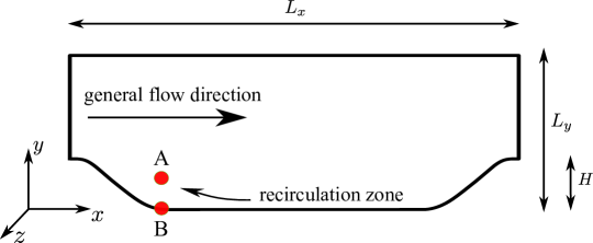
Figure 2: Domain shape for the flow in the channel with periodic hills. The $x$-, $y$- and $z$-coordinates are aligned with the streamwise, wall-normal, and spanwise directions, respectively. All dimensions are normalized by $H$ with $L_{x}/H=9$ and $L_{y}/H=3.036$. Two typical locations A ($x/H=2.0,y/H=0.5$) and B ($x/H=2.0,y/H=0.01$) are marked in the figure.

In the physics-based approach the variance fields $\sigma(x)$ for generating random perturbation fields $\Delta\xi(x)$, $\Delta\eta(x)$, $\Delta\log k(x)$, and $\Delta\varphi_{i}(x)$ ($i=1,2,3$) represent the magnitude of injected uncertainties. In the RMT approach the dispersion parameter $\delta(x)$ determines the variance of perturbations directly in the set $\mathbb{M}_{3}^{+}$ of positive definite matrices. To ensure that the distributions of perturbed Reynolds stresses from the two approaches are comparable, the amount of perturbation needs to be consistent with each other. Therefore, we estimate the dispersion parameter field $\delta(x)$ based on the samples of Reynolds stresses obtained in the physics-based approach with the given variance $\sigma(x)$. Although the physics-based approach is more flexible to specify different variances for the six discrepancy fields, it is difficult to determine how large the variance of each variable should be relative to each other. To be consistent with Xiao et al. [10], the Gaussian random fields for $\Delta\xi$, $\Delta\eta$, $\Delta\log k$, and $\Delta\varphi_{i}$ ($i=1,2,3$) share the same variance field $\sigma(x)$. Since the aim of this work is to compare the two approaches, we choose a constant variance field to avoid the complexity caused by spatial variations of the perturbation variances. We investigate two groups of cases with different magnitudes of perturbation. For cases Phy1 and RM1, a relatively small constant variance field $\sigma=0.2$ is used in the physics-based approach, and the corresponding dispersion parameter field $\delta(x)$ is estimated in the RMT approach. For cases Phy2 and RM2, a larger constant variance field $\sigma=0.6$ is applied. Since all results below are presented in degrees, we note that the variances $\sigma=0.2$ and $\sigma=0.6$ here for the Euler angles are in radian, which correspond to $12^{\circ}$ and $34^{\circ}$, respectively. For all cases, 30 modes are used in Karhunen–Loeve expansion to capture more than $90\%$ of the variance of the Gaussian random field. To reflect the anisotropy of the flow, an anisotropic yet spatially uniform length scale ($l_{x}/H=2$ and $l_{y}/H=1$) is used in the correlation kernel. To adequately represent the prior distribution of Reynolds stresses, 10,000 samples are drawn. The computational parameters are summarized in Table 1.

Table 1: Mesh and computational parameters used in the flow over periodic hills.

Parameters	Phy 1	RM 1	Phy 2	RM 2
variance/dispersion(a)	$\sigma=0.2$	see note (a)	$\sigma=0.6$	see note (a)
Karhunen–Loeve mesh	$50\times 30$
RANS mesh	$50\times 30$
number of modes $N_{\textrm{KL}}$	30
correlation length scales(b)	$l_{x}/H=2$, $l_{y}/H=1$
number of samples	10,000

3.2 Results and Discussions

Two groups of comparisons between the physics-based approach and the RMT approach are conducted with the samples drawn by the Monte Carlo method. In each case, the samples of Reynolds stress field $[\mathbf{R}(x)]$ are obtained by using both the physics-based algorithm described in Section 2.1 and the RMT approach in Section 2.2. The objective of this study is to gauge the prior specified in the physics-based approach by using the results of the RMT approach. Therefore, all the sampled Reynolds stresses are mapped to their physical dimensions, i.e., shape parameter (in Barycentric coordinates $C_{1},C_{2},C_{3}$ and natural coordinates $\xi,\eta$), magnitude $k$, and the Euler angles ($\varphi_{1}$, $\varphi_{2}$, and $\varphi_{3}$), to facilitate the comparison. Moreover, the decomposition into physical components also allows visualization of the distribution of random tensor fields. The marginal distributions of all components are investigated at two typical points: (1) point A located at $x/H=2.0$ and $y/H=0.5$ and (2) point B located at $x/H=2.0$ and $y/H=0.01$, indicated in Fig. 2. Point A is a generic point in the recirculation region, and point B is a near-wall point with two-dimensional turbulence representing limiting states.

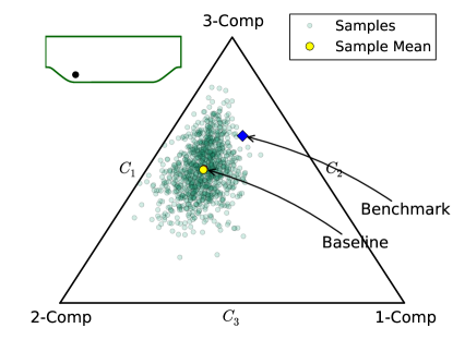
(a) Case Phy1, $\sigma=0.2$

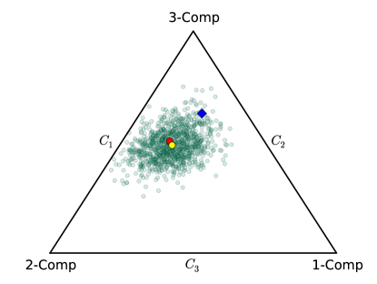
(b) Case RM1, $\sigma=0.2$

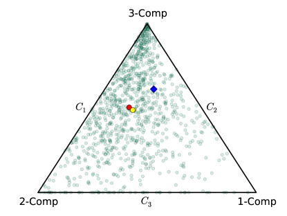
(c) Case Phy2, $\sigma=0.6$

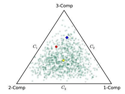
(d) Case RM2, $\sigma=0.6$

Figure 3: Scatter plots of the Reynolds stress samples projected to the Barycentric coordinates for point A ($x/H=2.0,y/H=0.5$) located in the recirculation region. Panels (a) and (b) compare the two approaches with small perturbation ($\sigma=0.2$), while panels (c) and (d) show the comparison with large perturbation ($\sigma=0.6$). The benchmark state is plotted as blue square, which is located to the upper right of the baseline result.

We first investigate the distributions of shape parameters of the Reynolds stress tensors in Barycentric coordinates, which have clear physical interpretations (see Fig. 1). The perturbed Reynolds stresses at the generic point A are sampled and projected onto the Barycentric triangle. The scatter plots of these samples for all cases are shown in Fig. 3. We can see that the baseline RANS-predicted Reynolds stress at this generic point is located in the interior of the triangle, while the benchmark result is located to the upper right of the baseline result. For all cases considered here, all samples fall inside the Barycentric triangle, demonstrating that the realizability is guaranteed in both approaches. The scatterings of samples in Figs. 3a and 3b are comparable, and this is also the case for Figs. 3c and 3d, indicating that the dispersion parameters $\delta$ estimated with the corresponding variances $\sigma$ are acceptable. The samples are still scattered around the baseline state, especially when the perturbation variance is small ($\sigma=0.2$). It shows that the sample mean overlaps with the baseline state in Fig. 3a. When the variance increases ($\sigma=0.6$), the mean value slightly deviates from the baseline state (comparing Figs. 3a and 3c). This deviation is markedly amplified in the RMT approach (Fig. 3d), suggesting that although the mean of perturbed Reynolds stresses is assumed to be the baseline result in the RMT approach, the mean is not preserved during the projection to the Barycentric coordinates. As the perturbation becomes large, the constraint of realizability leads to this significant deviation. Another notable difference between the results of two approaches lies in the shape of sample scattering. The scattering in case Phy1 is more elliptical-like with a large amount of samples spreading along the plain strain line (Fig. 3a), while in case RM1 the samples are scattered more circularly (Fig. 3b). When the perturbation is large ($\sigma=0.6$), we can see that in both cases Phy2 and RM2 the scatterings of samples show significant influence from the boundaries. In the results of the physics-based approach, a number of samples fall on the edges of the triangle, and a large number of samples are clustered near the top vertex (Fig. 3c). In contrast, in the RMT approach the samples are dispersed within the triangle without such clustering, and the frequency of occurrences decreases near the edges (Fig. 3d).

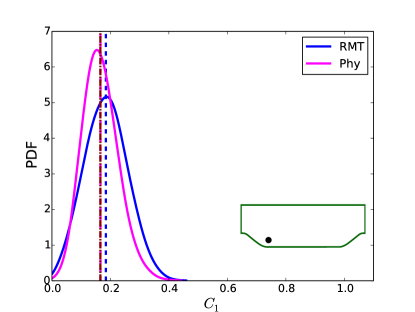
(a) cases Phy1 and RM1, $\sigma=0.2$

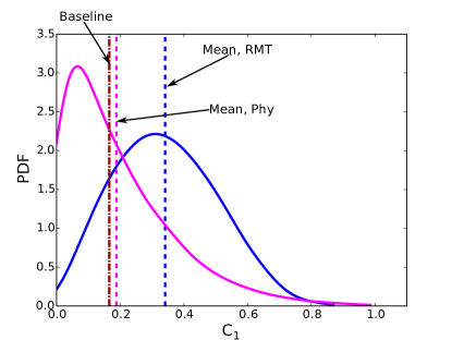
(b) cases Phy2 and RM2, $\sigma=0.6$

Figure 4: Probability distributions of the perturbed Barycentric coordinate $C_{1}$ for point A ($x/H=2.0,y/H=0.5$) located in the recirculation region. The results from the physics-based approach and the RMT approach are compared in the same plot. Panels (a) and (b) show the comparison at perturbation variances of $\sigma=0.2$ (cases Phy1 and RM1) and $\sigma=0.6$ (cases Phy2 and RM2), respectively.

Detailed comparison can be conducted by examining the marginal distributions of shape parameters in Barycentric coordinates $C_{1}$, $C_{2}$, and $C_{3}$. In Fig. 4 we present the probability density function (PDF) of $C_{1}$ for cases Phy1 and RM1 and cases Phy2 and RM2. Since $C_{2}$ and $C_{3}$ are correlated and have the similar characteristics as $C_{1}$, thus are omited for brevity. When the variance $\sigma$ is 0.2, the distributions obtained in both approaches are Gaussian, and the sample means are close to the baseline result. As the variance $\sigma$ increases to 0.6, both distributions deviate from Gaussian. In the physics-based approach the mode of samples (at peak of PDF) moves towards $C_{1}=0$ and the sample mean increases slightly compared to the baseline results. This is caused by the scheme used to impose the realizability constraint in the physics-based approach, where the samples falling outside the triangle are capped to the boundaries of natural coordinates (the four edges shown in Fig. 1b). Moreover, the samples spreading within the upper area of the natural coordinate square are squeezed in Barycentric triangle because of the mapping between the two coordinates. However, in the RMT approach the realizability of the Reynolds stress tensor $[\mathbf{R}]$ is guaranteed mathematically and no additional constraints are imposed due to the coordinates mapping. More precisely, the positive semi-definiteness of the normalized random matrix $[\mathbf{G}]$ is guaranteed by constructing from its Cholesky factor $[\mathbf{L}]$ (see Eq. 8). As a result, the distribution of $C_{1}$ is close to Gamma distribution with the sample mean increased compared to the baseline result. Based on the observations and discussions above, we find the bounding method used and the mapping between natural coordinate and Barycentric coordinate used in physics-based approach introduce some artificial constraints into the prior of Reynolds stresses. Therefore, it is better to specify Gaussian distributed perturbations of shape parameters in Barycentric coordinate to achieve maximum entropy for a generic location away from the wall.

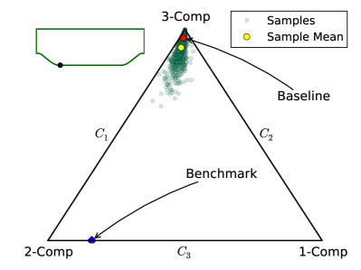
(a) Case Phy1, $\sigma=0.2$

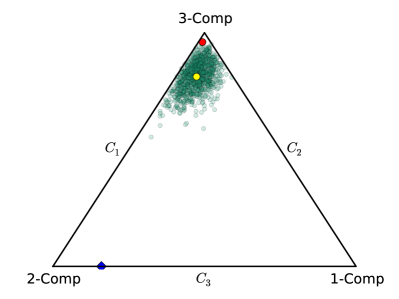
(b) Case RM1, $\sigma=0.2$

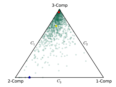
(c) Case Phy2, $\sigma=0.6$

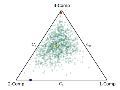
(d) Case RM2, $\sigma=0.6$

Figure 5: Scatter plots of the Reynolds stress samples projected to the Barycentric coordinates for point B ($x/H=2.0,y/H=0.01$) located in the recirculation region. Panels (a) and (b) compare the two approaches with small perturbation ($\sigma=0.2$), while panels (c) and (d) show the comparison with large perturbation ($\sigma=0.6$). The benchmark state is plotted as blue square, which is located on the bottom edge of the triangle, indicating two-component turbulence.

It is also interesting to study the a point located close to the wall. Similarly, the comparisons of scatter plots of Reynolds stress samples at point B are presented in Fig. 5. It shows that the benchmark truth is located on the bottom edge of the triangle, indicating the two-component limiting state. This is because the velocity fluctuations in wall-normal direction are suppressed by the blocking of bottom wall of the channel. In contrast, RANS-predicted Reynolds stress is close to the three-component isotropic state, located near the top vertex of the triangle. For the point B at the near wall location, the sample scatterings in all four cases are markedly affected by the boundaries of the triangle, and the sample means move downwards. This is due to the fact that the distances from the baseline state to the boundaries are relatively small compared to the perturbations, and thus the perturbed states are significantly affected by these constraints. However, the influences caused by the constraints imposed in the two approaches are different. In the case with a small variance $\sigma=0.2$ (case Phy1, Fig. 5a), the samples are largely clustered near the top vertex and the scattering is squeezed artificially in the physics-based approach. Although enough samples are drawn, very few of them fall in the areas near the two side edges. In contrast, the samples in the RMT approach are dispersed within the entire upper area of the triangle and better explored the spanned uncertainty space (case RM1, Fig. 5b). When the variance is large ($\sigma=0.6$, case Phy2, Fig. 5c), the capping scheme used to ensure realizability in the physics-based approach has a more pronounced effect on the obtained sample distribution. Specifically, about one half of the samples are capped to the edges or the vertices of the Barycentric triangle, leading to deteriorated sample effectiveness.

The differences of perturbations in shape parameters between the two approaches are discussed above for two typical points A and B of the channel. In order to quantitatively explore the spatial variation of the difference between the two approaches, we calculate the Kullbck-Leibler divergence of the distribution obtained by the physics-based approach from the distribution obtained by the RMT approach. The Kullbck-Leibler divergence (also known as relative entropy) of $q$ from $p$ is a measure of the difference between two probability densities $p$ and $q$, which is defined as [22]

$$D_{KL}(p||q)=\int_{\mathbb{I}}\log\frac{p(\vartheta)}{q(\vartheta)}d\vartheta,$$ (14)

where $\vartheta$ denotes the parameter, and $\mathbb{I}$ is the parameter space. The Kullbck-Leibler divergence is analogous to a “distance” between two distributions, but it is not a distance measure since it does not preserve the symmetry in $p$ and $q$. More intuitively, the Kullbck-Leibler divergence of $q$ from $p$ can be interpreted as the measure of the information gained from the distribution $p$ to distribution $q$. The Kullbck-Leibler divergence is calculated to reflect the additional information introduced in the physics-based approach based on the maximum entropy distribution obtained with the RMT approach. Figure 6 shows the spatial profiles of Kullbck-Leibler divergence for the shape parameter $C_{1}$. The profiles are shown at eight streamwise locations, $x/H=1,\cdots,8$, and the dashed black lines are plotted to indicate the axis of $D_{KL}=0$. The geometry of the physical domain is also plotted to facilitate visualization. To clearly show the characteristics of the profiles, a larger scale factor of 0.9 is used in Fig. 6a, while a smaller scale factor of 0.3 is used in Fig. 6b. When the variance is small ($\sigma=0.2$), the Kullbck-Leibler divergence is also small over the entire domain (Fig. 6a), suggesting that the distributions of shape parameters obtained from the physics-based approach are similar to those obtained from the RMT approach. When we increase the perturbation variance ($\sigma=0.6$), the Kullbck-Leibler divergence becomes larger over the entire domain (Fig. 6b), indicating that the additional, artificial constraints introduced in the physics-based approach are significant with large perturbation. Moreover, both Figs. 6a and 6b show that the Kullbck-Leibler divergences for the locations near the wall are slightly larger than those at generic locations. As has been discussed above, the baseline RANS-predicted Reynolds stress near the wall is close to three-component isotropic limiting state. This results in the fact that the perturbation is large compared to the distance from baseline state to the boundary of the triangle, and thus more artificial information is introduced in the physics-based approach at the near-wall regions. It is noted that the $D_{KL}$ is also large at $y/H=2.5$, which is because the baseline state is closer to the top vertex of triangle at $y/H=2.5$. All these observations are consistent with the discussion above for the two typical points A and B.

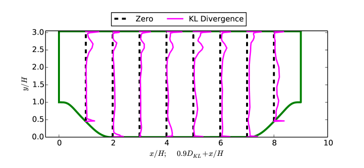
(a) $\sigma=0.2$

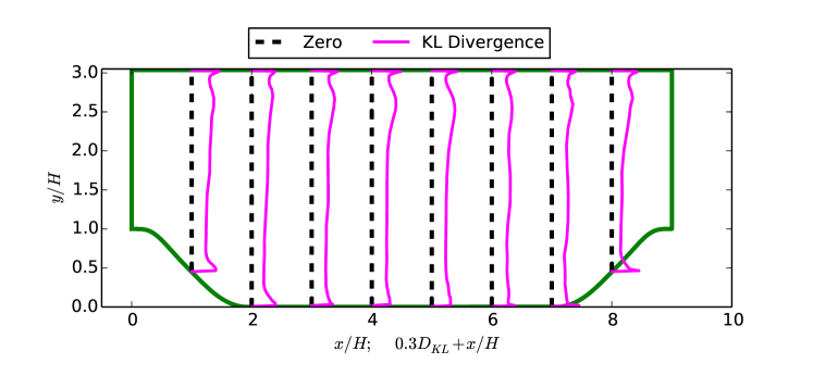
(b) $\sigma=0.6$

Figure 6: Kullbck-Leibler divergence profiles with (a) $\sigma=0.2$ and (b) $\sigma=0.6$. The profiles are shown at eight streamwise locations $x/H=1,\cdots,8,$ and the reference lines, $D_{KL}=0+x/H$, are also plotted. Note that in panel (a), since the scale of $D_{KL}$ is quite smaller than that of panel (b), a larger scale factor of 0.9 is used in (a), while a smaller scale factor of 0.3 is used in (b).

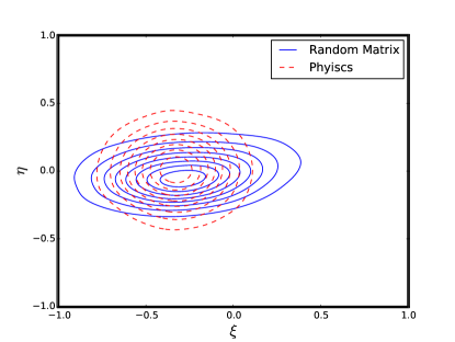
(a) Phy1 and RM1 ($\sigma=0.2$)

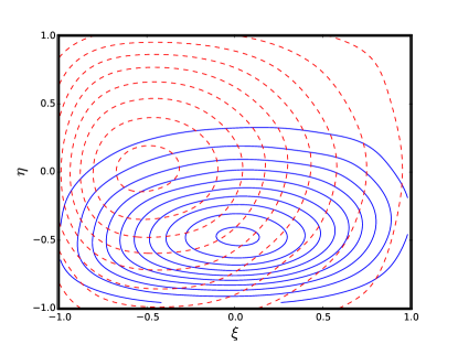
(b) Phy2 and RM2 ($\sigma=0.6$)

Figure 7: Comparisons of probability density contours of natural coordinates ($\xi$ and $\eta$) obtained from the physics-based approach and the RMT approach at point A ($x/H=2.0,y/H=0.01$. Panel (a) and (b) are with the perturbations $\sigma=0.2$, and $\sigma=0.6$, respectively.)

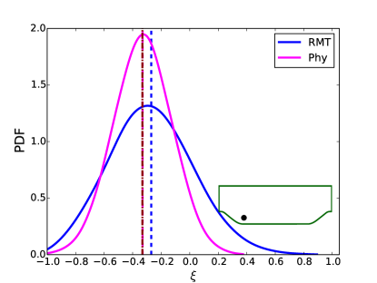
(a) PDF of $\xi$, $\sigma=0.2$

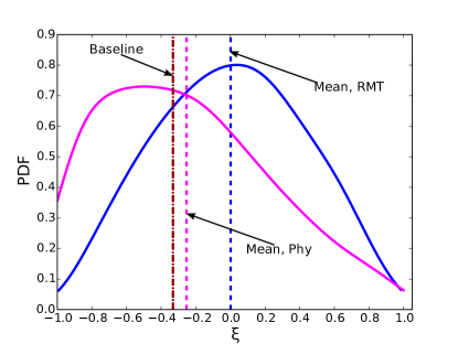
(b) PDF of $\xi$, $\sigma=0.6$

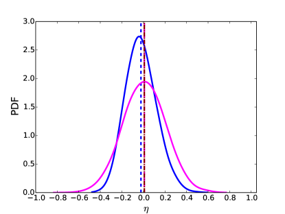
(c) PDF of $\eta$, $\sigma=0.2$

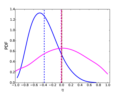
(d) PDF of $\eta$, $\sigma=0.6$

Figure 8: Distributions of the perturbed natural coordinates $\xi$ and $\eta$ for point A ($x/H=2.0,y/H=0.5$) located in recirculation region. The results from the physics-based approach and the RMT approach are compared in the same plot. Panels (a) and (b) show the comparison of $\xi$ at perturbation variances of $\sigma=0.2$ and $\sigma=0.6$, respectively. Panels (c) and (d) show the comparison of $\eta$ at perturbation variances of $\sigma=0.2$ and $\sigma=0.6$, respectively.

The analysis above suggests that imposing Gaussian perturbation directly in Barycentric coordinates (as oppose to the natural coordinates) leads to a distribution closer to maximum entropy. However, the perturbations were imposed in natural coordinates by Xiao et al. [10] due to practical considerations. Since the Barycentric coordinates $C_{1}$, $C_{2}$, and $C_{3}$ are correlated, and the triangle boundary edges pose difficulties on the capping scheme, the natural coordinates $\xi$ and $\eta$ are preferred for implementation purposes. In order to determine proper perturbations in $\xi$ and $\eta$ to obtain prior with maximum entropy in the physics-based approach, we also need to map the Barycentric coordinates to the natural coordinates in the RMT approach. With the samples of natural coordinates $\xi$ and $\eta$, their joint density can be estimated with Gaussian kernels. Figures 7a and 7b show the comparison of joint PDF contours obtained by the two approaches with variances $\sigma=0.2$ and $\sigma=0.6$, respectively. Moreover, the comparisons of marginal distributions of $\xi$ and $\eta$ are also plotted in Fig. 8. When the perturbation is small ($\sigma=0.2$), the contours in both cases Phy1 and RM1 are elliptical, indicating the joint distributions are approximately Gaussian (Fig. 8a). However, a notable difference between the results of the two approaches lies on the shapes of the contours. The elliptical contour in the RMT approach is anisotropic with larger variance for $\xi$ but smaller for $\eta$. In the physics-based approach the contour is circular due to the artificial choice of the same perturbation variance for both $\xi$ and $\eta$. Therefore, to achieve the prior with approximate maximum entropy, the perturbation in $\xi$ should be larger than that in $\eta$ for this flow of concern. More details can be found in their marginal distributions (Figs. 8a and 8c). For both approaches with small perturbation ($\sigma=0.2$) in Reynolds stress, the marginal distributions for $\xi$ and $\eta$ are Gaussian. With the RMT approach, the perturbation variance of $\xi$ is approximately twice as large as that with the physics-based approach, while the perturbation of $\eta$ is slightly smaller than that with the physics-based approach. However, when the perturbation is large ($\sigma=0.6$), the joint distribution of $\xi$ and $\eta$ obtained by both approaches are no longer Gaussian, and the density contours are influenced by the boundaries (Fig. 7b). Especially in case Phy2 the shape of the contour clearly follows the rectangular edges. Unlike the physics-based approach, the shape of the contour obtained with the RMT approach is less affected by the boundaries. Detailed comparisons are shown by the corresponding marginal distributions. All the distributions are distorted compared to the Gaussian PDF (Gaussian density with the sample mean and variance). The distortions in the physics-based approach are due to the fact that large number of unrealizable samples are capped onto the edges. However, in the RMT approach the sample means of $\xi$ and $\eta$ significantly deviate from the baseline results. The mean of $\xi$ moves towards the middle point ($\xi=0$) of $\xi$ range, while the mean of $\eta$ moves towards approximate one third ($\eta=-0.4$) of the $\eta$ range $[-1,1]$. This sample mean point ($\xi=0.0$, $\eta=-0.4$) is close to the centroid of the triangle when mapped back to the Barycentric coordinates. Moreover, the distributions are approximately bounded Gaussian that satisfies the realizability constraint mathematically. The deviation of sample mean from the baseline when the perturbation is large can be interpreted intuitively. Since the large perturbation of Reynolds stress implies less confidence on the baseline prediction, it is reasonable to adjust the sample mean to the centroid of triangle to have a better sample scattering over the entire triangle. The results shown in Figs. 7a, 8a, and 8c suggest that, for a generic point away from the wall, imposing small perturbations on $\xi$ and $\eta$ with Gaussian distributions lead to Reynolds stresses that are very close to the maximum entropy distribution. This observation lends partial support to the choice of prior distributions made in [10]. However, to achieve the maximum entropy prior, the perturbation variance of $\xi$ should be approximately twice as large as that of $\eta$. When the perturbation of Reynolds stress is large, to achieve maximum entropy we should first shift the baseline $\xi$ and $\eta$ to the centroid of the Barycentric triangle, and then perturb the shifted baseline results with bounded Gaussian distribution.

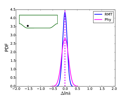
(a) $\sigma=0.2$, location A

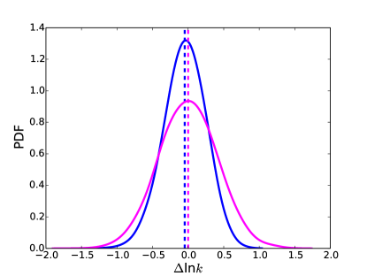
(b) $\sigma=0.6$, location A

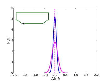
(c) $\sigma=0.2$, location B

(d) $\sigma=0.6$, location B

Figure 9: Distributions of the perturbations ($\Delta\log k$) in turbulence kinetic energy in logarithmical scale. The upper two panels show the results at point A ($x/H=2.0,y/H=0.5$), while the lower two panels show the results at point B ($x/H=2.0,y/H=0.01$). The results from physics-based approach and random matrix theoretic approach are compared in the same plot. The sample mean of the physics-based approach overlaps with that of the RMT approach (denoted as blue (dark) dashed line and pink (grey) dashed line, respectively)

In addition to the shape of Reynolds stress, its magnitude i.e., the turbulence kinetic energy (TKE), is also difficult to predict in RANS models. In the physics-based approach, the perturbations in turbulence kinetic energy are specified to be log-normally distributed. To evaluate if this specification is justified, we compared the TKE perturbations in logarithmic scale $\Delta\log k$ obtained from the two approaches. The marginal distributions of $\Delta\log k$ with different perturbation levels ($\sigma=0.2$ and $\sigma=0.6$) at points A and B are presented in Fig. 9. In both the physics-based and RMT approaches, the perturbations in TKE obey the log-normal distribution, since all the PDFs of $\Delta\log k$ shown in Fig. 9 are close to the Gaussian distributions. This conclusion is also true for the cases with larger perturbations (cases Phy2 and RM2, $\sigma=0.6$) as well. Therefore, introducing a log-normally distributed prior for TKE discrepancies leads to a distribution of Reynolds stresses that is close to the one with maximum entropy. This lends support to the choice of prior in the physics-based approach [10]. Another interesting observation in Fig. 9 is that the spreading of $\Delta\log k$ samples with the RMT approach is slightly smaller than that with physics-based approach. As mentioned above, in the physics-based approach the same variance field $\sigma(x)$ is shared by the perturbations of six variables ($\xi$, $\eta$, $k$, $\varphi_{1}$, $\varphi_{2}$, $\varphi_{3}$) due to the lack of prior knowledge. However, this assumption is another constraint imposed in the physics-based approach. Based on the comparisons in Fig. 9, we find that to achieve the maximum entropy, the perturbation variance for each parameter should be different. It suggests that a relatively smaller variance (approximate 50% of that for shape parameter) is proper for the perturbation of TKE in logarithmic scale for this flow of concern.

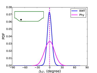
(a) $\sigma=0.2$, at location A

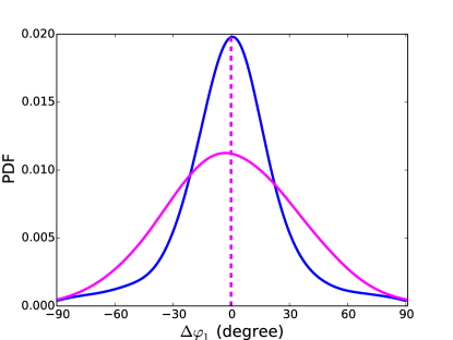
(b) $\sigma=0.6$, at location A

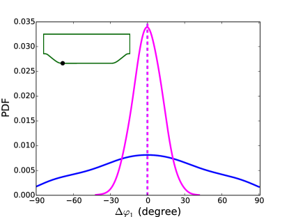
(c) $\sigma=0.2$, at location B

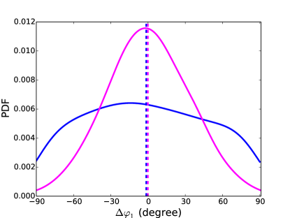
(d) $\sigma=0.6$, at location B

Figure 10: Distributions of the perturbations ($\Delta\varphi_{1}$) in orientation. The upper two panels show the results at point A ($x/H=2.0,y/H=0.5$), while the lower two panels show the results at point B ($x/H=2.0,y/H=0.01$). The results from Physics-based approach and random matrix theoretic approach are compared in the same plot. The sample mean of the physics-based approach overlaps with that of the RMT approach (denoted as blue (dark) dashed line and pink (grey) dashed line, respectively)

While the orientations of the Reynolds stresses have not been perturbed in [10], in this study they are perturbed with the same variance $\sigma$ as that of other variables. However, if or how large the orientation should be perturbed are model choices in the physics-based approach. Without further physical information, it is difficult to determine the variance of perturbations in angles. To examine this issue, the marginal distributions of angle discrepancies obtained from both approaches are compared. Fig. 10 shows the comparison of PDF of $\Delta\varphi_{1}$ with different perturbation magnitudes at the points A and B. The perturbations in $\varphi_{2}$ and $\varphi_{3}$ have similar characteristics as that of $\varphi_{1}$, and thus they are omitted for brevity. We can see that to achieve the maximum entropy the orientation of the tensor should also be perturbed. Similarly to the perturbations in TKE, the sample mean of $\Delta\varphi_{1}$ is zero for all cases. This indicates that the sample means in tensor magnitude and orientation are the same as those of baseline RANS prediction, since there are no physical constraints on TKE and Euler angles (except for the range $[-\pi,\pi]$ specified in the definition). In the physics-based approach, the PDFs are Gaussian for all cases, since Gaussian random fields are employed to model the discrepancies in angles. For the generic point A, the distribution of $\Delta\varphi_{1}$ obtained from the RMT approach is also close to Gaussian when the perturbation is small (Fig. 10a). However, the scattering of samples is smaller than what we specified in the physics-based approach, and most of the perturbations are within $\pm 20$ degrees. As the perturbation magnitude is enlarged, the PDF obtained in the RMT approach is peaked compared to the Gaussian distribution (Fig. 10b). Consequently, most samples are with small perturbations (smaller than $30$ degrees). However, for the point B located close to the wall, the variances of $\Delta\varphi_{1}$ in cases RM1 and RM2 are much larger, even though the perturbation of tensor is small (Fig. 10c). In the RMT approach the distribution of $\Delta\varphi_{1}$ is flatter than the corresponding Gaussian distribution, and most of the perturbations $\Delta\varphi_{1}$ are larger than $60$ degrees. Especially when the dispersion parameter is large (i.e., $\delta(x)$ corresponding to $\sigma=0.6$), the PDF of $\Delta\varphi_{1}$ significantly deviates from the Gaussian distribution (Fig. 10d). The observations above imply that, to obtain a maximum entropy prior, the perturbations variance in orientation should be spatially non-stationary. For this specific flow, smaller perturbations (with 30 degrees) should be used for a generic point away from the way, while larger perturbations are appropriate for the near wall locations.

The results shown above suggest that, when the RANS predictions are relatively reliable with small perturbations needed, using normally distributed perturbations for each of the six physical variables is a good choice to obtain the Reynolds stress prior that is close to the one with maximum entropy. This observation can be related to the case of a scalar random variable. With the constraints of a specified mean and variance, the maximum entropy distribution of a scalar random variable is the Gaussian distribution [23]. That is, by choosing Gaussian distributions for the discrepancies of Reynolds stresses in the physics-based approach, the maximum entropy distribution is achieved for each individual physical variables (magnitude, shape, orientation). The variance of each variable is, however, chosen by the user and is thus a modeling choice. In contrast, in the RMT approach the maximum entropy is achieved for the distribution of the Reynolds tensor. Consequently, the relative magnitude of the variance for each variable is implied based on the maximum entropy principle and is not a modeling choice of the user. However, it is worth pointing out that, although we use the results of the RMT approach as the golden standard for gauge the physics-based approach, the correlation structure (see Eq. 13) and corresponding Karhunen-Loeve modes used to represent the random field are still modeling choices, which also may introduce artificial constraints. In summary, one can consider that in the RMT approach, maximum entropy is achieved for the pointwise distribution of the Reynolds stresses at each location $x$, but not necessarily for the random field $[\mathbf{R}(x)]$. In the physics based approach, maximum entropy is achieved for the pointwise distribution for individual physical variables ($k$, $\xi$, $\eta$ etc.) but not necessarily for the Reynolds stress tensor $[\mathbf{R}]$ or the field $[\mathbf{R}(x)]$.

4 Conclusion

Quantification of the uncertainties originating from the modeled Reynolds stresses is crucial when the RANS simulations are applied in the decision-making process. One of the challenges in current form of the physics-based model-form uncertainty quantification framework is to specify proper priors for the physical variables (shape, magnitude, and orientation). It is difficult to determine if or how much additional information is introduced into the priors specified in the physics-based approach. To evaluate the priors and gain insights on proper specification of the priors, the random matrix theoretic approach with the maximum entropy principle is used in this work. By comparing the distributions of shape, magnitude, and orientation variables obtained from the two approaches, we find some useful guidelines of prior specification for these wall-bounded flows with separations. For the shape parameters, the Gaussian distributed perturbations in Barycentric coordinate is better to achieve maximum entropy. The mapping between the Barycentric coordinate to the natural coordinate may introduces some artificial constraints, especially when the RANS prediction is less reliable (large perturbation needed). For the turbulence kinetic energy, introducing log-normally distributed perturbations leads to a distribution of Reynolds stresses that is close to the one with the maximum entropy. This observation lends support to the choice of prior in [10]. Moreover, different variance fields for the perturbations of the Reynolds stress shape parameters $\xi$, $\eta$, and the magnitude (turbulence kinetic energy) $k$ are required to achieve maximum entropy. Specifically, for the flow over periodic hills examined in this study the variance of $\xi$ should be larger than that of $\eta$, and the perturbation of $\log k$ should be relatively small. Finally, it suggests that the uncertainties should be also injected in the orientation of Reynolds stresses represented by Euler angles. For a generic location away from the wall, the perturbations of Euler angles should be small, while larger perturbations should be added for the near wall locations. The conclusion can be used as a guidance for the objective prior specification in the physics-based, Bayesian uncertainty quantification framework.

Appendix A Summary of Algorithms of The Physics-Based Approach

1. Decomposition to physically meaningful dimension and expansion of given marginal distributions

   1. Perform the baseline RANS simulation to obtain the baseline (mean) Reynolds stress $[\underline{R}]$.

   2. Perform the transformation $[\underline{R}]\mapsto(\tilde{\xi}^{rans},\,\tilde{\eta}^{rans},\,\tilde{k}^{rans},\,\tilde{\varphi}_{1}^{rans},\,\tilde{\varphi}_{2}^{rans},\,\tilde{\varphi}_{3}^{rans})$.

   3. Compute Karhunen–Loeve expansion to obtain basis set $\{\phi_{\alpha}(x)\}_{\alpha=1}^{N_{kl}}$, where $N_{kl}$ is the number of modes retained.

2. Sampling and reconstruction of physical variable fields for Reynolds stresses:

   1. Sample six independent coefficient vectors $\{\boldsymbol{\omega}_{\beta}\}_{\beta=1}^{N}$ for the six discrepancy fields (i.e., $\Delta\xi,\Delta\eta,\Delta\log{k},\Delta\varphi_{1},\Delta\varphi_{2}$, and $\Delta\varphi_{3}$ ), where $N$ is the sample size.

   2. Reconstruct the six discrepancy fields with the six independent coefficient samples $\{\boldsymbol{\omega}_{\beta}\}_{\beta=1}^{N}$ and Karhunen–Loeve modes. Note that the variance field $\sigma(x)$ is the same for the six random fields.

   3. Obtained samples of Reynolds stress field $[\mathbf{R}]$ via mapping $(\xi,\,\eta,\,k,\,\varphi_{1},\,\varphi_{2},\,\varphi_{3})\mapsto[R]$

3. Propagation the Reynolds stress to QoIs via RANS equations

   1. Use the obtained sampled Reynolds stress to velocity and other QoIs by solving the RANS equations.

   2. Post-process the obtained velocity and QoI samples to obtain statistical moments.

Appendix B Summary of Algorithms of The RMT Approach

Given the mean Reynolds stress field $[\underline{R}(x)]$ (e.g., from RANS-predicted results) along with the correlation function structure of the random upper triangle matrix field $[\mathbf{L}](x)$, the following procedure is performed:

1. Expansion of given marginal distributions and covariances kernels:

   1. Perform the Cholesky factorization of the mean Reynolds stresses $[\underline{R}]$ at each cell as $[\underline{R}]=[\underline{L}_{R}]^{T}[\underline{L}_{R}]$, which yields field $\underline{L}_{R}(x)$ of upper triangular matrices.

   2. Perform Karhunen–Loeve expansion for the kernel function by solving the Fredholm equation to obtain eigenmodes.

   3. For off-diagonal terms of matrix $[\mathbf{L}]$, perform polynomial expansion (PCE) of the Gamma marginal PDF at each cell. PCE Coefficients $U_{\beta}$ are obtained from

      $$U_{\beta}=\frac{\langle\mathbf{u}{\Psi}_{\beta}\rangle}{\langle{\Psi}_{\beta}^{2}\rangle}\\ =\frac{1}{\langle{\Psi}_{\beta}^{2}\rangle}\int_{\Omega}F_{\mathbf{u}}^{-1}[F_{\mathbf{w}}(w)]\;{\Psi}_{\beta}({w})\;p_{\text{\tiny{w}}}(w)dw,$$ (15)

      where $\langle\boldsymbol{\Psi}_{\beta}^{2}\rangle$ is the variance of $i$^th order polynomial of standard Gaussian random variable $\mathbf{w}$; $F_{w}(\mathbf{w})$ and $p_{\text{\tiny{w}}}$ are the cumulative distribution function (CFD) and PDF, respectively, of $\mathbf{w}$; $\Omega$ is the sample space of $\mathbf{w}$; $F_{\mathbf{u}}$ and $F_{\mathbf{u}}^{-1}$ are the CDF and its inverse, respectively, of random variable $\mathbf{u}$. The index $\beta$ is from $1$ to $N_{p}$, and $N_{p}$ is the number of polynomials retained in the expansion.

2. Sampling and reconstruction of random matrix fields for Reynolds stresses:

   1. For each element $\mathbf{L}_{ij}$ of the random matrix field $[\mathbf{L}]$, independently draw $N_{kl}$ sample from the standard Gaussian distribution $\omega_{ij,\alpha}$ where $\alpha=1,\cdots,N_{kl}$, e.g., with random sampling or Latin hypercube sampling method.

   2. Synthesize realizations of the off-diagonal terms based on Karhunen–Loeve expansion:

      $$\mathbf{w}_{ij}(x) =\sum_{\alpha=1}^{N_{\textrm{KL}}}\,\phi_{\alpha}(x)\;\boldsymbol{\omega}_{\alpha}\quad\textrm{with}\quad i<j$$

      $$\mathbf{L}_{ij}(x) =\sigma_{d}\mathbf{w}_{ij}(x)$$

   3. Synthesize the realizations of the diagonal terms based on Karhunen–Loeve and PCE expansions:

      $$\mathbf{u}_{i}(x)=\sum_{\beta=0}^{N_{p}}U_{\beta}(x)\Psi_{\beta}(\mathbf{w}_{ii}(x))$$

      where the Gaussian random field sample $\mathbf{w}_{ii}(x)$ obtained in the previous step is used.

   4. Synthesize the diagonal terms of matrix $[\mathbf{L}]$ from $\mathbf{L}_{ii}(x)=\sigma_{d}\sqrt{2\mathbf{u}_{i}}$, where $i=1,2,3$.

   5. Reconstruct random normalized matrix $[\mathbf{G}]$ from $[\mathbf{G}]=[\mathbf{L}]^{T}[\mathbf{L}]$ and then reconstruct the Reynolds stress tensor $[\mathbf{R}]$ from $[\mathbf{R}]=[\underline{L}_{R}]^{T}[\mathbf{G}][\underline{L}_{R}]$.

3. Propagation the Reynolds stress field through the RANS solver to obtain velocities and other QoIs:

   1. Use the obtained sampled Reynolds stress to velocity and other QoIs by solving the RANS equations.

   2. Post-process the obtained velocity and QoI samples to obtain statistical moments.

Appendix C Nomenclature

Subscripts/Superscripts
$i$, $j$	tensor indices ($i,j=1,2,3$); repeated indices does not imply summation
$\alpha$, $\beta$	indices for terms in Karhunen–Loeve and polynomial chaos expansions
$l$	general index (modes etc.)
Sets, operators, and decorative symbols
$\mathbb{R}^{+}$	the set of all real positive number
$\mathbb{E}\{\cdot\}$	expectation of a random variable
$\mathbb{M}_{d}^{s}$	the set of all $d\times d$ symmetric matrices
$\mathbb{M}_{d}^{+}$	the set of all $d\times d$ symmetric, positive definite matrices
$\mathbb{M}_{d}^{+0}$	the set of all $d\times d$ symmetric, positive semi-definite matrices
$\operatorname{tr}$	trace of a matrix
$\operatorname{det}$	determinant of a matrix
$[\cdot]$	matrix
$\underline{\Box}$	mean value of variable $\Box$
$\bullet$	inner product of two (determistic) vectors
$\langle\cdot\rangle$	ensemble average/expectation of a random variable
$\|\cdot\|_{F}$	Frobenius norm
$\sum$	summation
$\prod$	product
Roman letters
$[A]$	anisotropy tensor of the Reynolds stress
$C$	Barycentric coordinates
$d$	dimension of matrices ($d=3$ implied unless noted otherwise)
$D_{KL}$	Kullbck-Leibler divergence
$\vec{e}_{1}$, $\vec{e}_{2}$, $\vec{e}_{3}$	orthonormal eigenvectors of Reynolds stress anisotropy $[A]$
$[E]$	orthonormal eigenvectors of Reynolds stress anisotropy $[A]$
$F$	cumulative distribution function
$[\mathbf{G}],[G]$	a positive definite matrix with identity matrix $[I]$ as its mean
$[I]$	identity matrix
$k$	turbulence kinetic energy
$K$	covariance kernel
$[\mathbf{L}],[L]$	an upper triangle matrix (e.g., obtained from Cholesky factorization)
$l$	length scale of Gaussian process
$\mathbf{N}$	Gaussian normal distribution
$N_{p}$	order of polynomial in the PCE expansion
$N_{kl}$	number of modes in KL expansion
$p,q$	probability density function
$[\mathbf{R}]$, $[R]$	(negative of) Reynolds stress tensor with $R_{ij}=\langle\mathbf{v}_{i}^{\prime}\mathbf{v}_{j}^{\prime}\rangle$
$\mathbf{v}_{i}^{\prime}$	the $i$th component of the fluctuation velocity (random variable)
$\mathbf{u}$	Gamma random variable used to define the diagonal terms of the Reynolds stress $\mathbf{L}_{\alpha\alpha}$
$U$	coefficients for the polynomial
$\mathbf{w}$	standard Gaussian random variable
$x$	spatial coordinate index
Greek letters
$\delta$	dispersion parameter (uncertainty of the random matrix)
$\sigma$	variance of Gaussian process
$\vartheta$	parameter
$\rho$	correlation
$\xi$, $\eta$	natural coordinates
$\Lambda$, $\lambda$	eigenvalues of anisotropy $[A]$
$\varphi$	Euler angle of Reynolds stress tensor
$\tilde{\omega},\phi$	eigenvalues and basis functions obtained from Karhunen-Loeve expansion
$\Psi_{j}$	$j$th order Hermite polynomial of standard Gaussian random variable $\mathbf{w}$

References

- [1] S. B. Pope, Turbulent flows, Cambridge university press, 2000.
- [2] T. Oliver, R. Moser, Uncertainty quantification for RANS turbulence model predictions, in: APS Division of Fluid Dynamics Meeting Abstracts, 2009.
- [3] L. Margheri, M. Meldi, M. Salvetti, P. Sagaut, Epistemic uncertainties in RANS model free coefficients, Computers & Fluids 102 (2014) 315–335.
- [4] W. Edeling, P. Cinnella, R. P. Dwight, H. Bijl, Bayesian estimates of parameter variability in the k– turbulence model, Journal of Computational Physics 258 (2014) 73–94.
- [5] W. Edeling, P. Cinnella, R. P. Dwight, Predictive RANS simulations via Bayesian model-scenario averaging, Journal of Computational Physics 275 (2014) 65–91.
- [6] M. Emory, R. Pecnik, G. Iaccarino, Modeling structural uncertainties in Reynolds-averaged computations of shock/boundary layer interactions, in: 49th AIAA Aerospace Sciences Meeting, 2011.
- [7] E. Dow, Q. Wang, Quantification of structural uncertainties in the k– turbulence model, AIAA Paper 1762 (2011) 2011.
- [8] M. Emory, J. Larsson, G. Iaccarino, Modeling of structural uncertainties in Reynolds-averaged Navier-Stokes closures, Physics of Fluids 25 (11) (2013) 110822.
- [9] C. Gorlé, G. Iaccarino, A framework for epistemic uncertainty quantification of turbulent scalar flux models for Reynolds-averaged Navier-Stokes simulations, Physics of Fluids (1994-present) 25 (5) (2013) 055105.
- [10] H. Xiao, J.-L. Wu, J.-X. Wang, R. Sun, C. J. Roy, Quantifying and reducing model-form uncertainties in Reynolds-Averaged Navier-Stokes simulations: An open-box, physics-based, bayesian approach, submitted. Available at http://arxiv.org/abs/1508.06315 (2015).
- [11] J.-X. Wang, J.-L. Wu, H. Xiao, Incorporating prior knowledge for quantifying and reducing model-form uncertainty in RANS simulations, submitted. Available at http://arxiv.org/abs/1512.01750 (2015).
- [12] S. Guiasu, A. Shenitzer, The principle of maximum entropy, The mathematical intelligencer 7 (1) (1985) 42–48.
- [13] E. T. Jaynes, Information theory and statistical mechanics, Physical review 106 (4) (1957) 620.
- [14] C. Soize, A nonparametric model of random uncertainties for reduced matrix models in structural dynamics, Probabilistic engineering mechanics 15 (3) (2000) 277–294.
- [15] S. Das, R. Ghanem, A bounded random matrix approach for stochastic upscaling, Multiscale Modeling & Simulation 8 (1) (2009) 296–325.
- [16] H. Xiao, J.-X. Wang, R. G. Ghanem, A random matrix approach for quantifying model-form uncertainties in turbulence modeling, to be submitted. Available at https://sites.google.com/a/vt.edu/hengxiao/papers (2016).
- [17] J.-L. Wu, J.-X. Wang, H. Xiao, A Bayesian calibration-prediction method for reducing model-form uncertainties with application in RANS simulations, submitted. Available at http://arxiv.org/abs/1510.06040 (2015).
- [18] S. Banerjee, R. Krahl, F. Durst, C. Zenger, Presentation of anisotropy properties of turbulence, invariants versus eigenvalue approaches, Journal of Turbulence 8 (32) (2007) 1–27.
- [19] H. Goldstein, Classical Mechanics, 2nd Edition, Addison-Wesley, 1980, see “The Euler Angles and Euler Angles in Alternate Conventions” in Chapter 4.4.
- [20] O. P. Le Maître, O. M. Knio, Spectral methods for uncertainty quantification: with applications to computational fluid dynamics, Springer, 2010.
- [21] S. Sakamoto, R. Ghanem, Polynomial chaos decomposition for the simulation of non-Gaussian nonstationary stochastic processes, Journal of engineering mechanics 128 (2) (2002) 190–201.
- [22] S. Kullback, Information theory and statistics, Courier Corporation, 1968.
- [23] S. Y. Park, A. K. Bera, Maximum entropy autoregressive conditional heteroskedasticity model, Journal of Econometrics 150 (2) (2009) 219–230.