Photoelectron spectra with Qprop and t-SURFF

Abstract

Calculating strong-field, momentum-resolved photoelectron spectra (PES) from numerical solutions of the time-dependent Schrödinger equation (TDSE) is a very demanding task due to the large spatial excursions and drifts of electrons in intense laser fields. The time-dependent surface flux (t-SURFF) method for the calculation of PES [L. Tao, A. Scrinzi, New Journal of Physics 14, 013021 (2012)] allows to keep the numerical grid much smaller than the space over which the wavefunction would be spread at the end of the laser pulse. We present an implementation of the t-SURFF method in the well established TDSE-solver Qprop [D. Bauer, P. Koval, Comput. Phys. Commun. 174, 396 (2006)]. Qprop efficiently propagates wavefunctions for single-active electron systems with spherically symmetric binding potentials in classical, linearly (along $z$) or elliptically (in the $xy$-plane) polarized laser fields in dipole approximation. Its combination with t-SURFF makes the simulation of PES feasible in cases where it is just too expensive to keep the entire wavefunction on the numerical grid, e.g., in the long-wavelength or long-pulse regime.

NEW VERSION PROGRAM SUMMARY

Manuscript Title: Photoelectron spectra with Qprop and t-SURFF
Authors: Volker Mosert, Dieter Bauer
Program Title: Qprop
Journal Reference:
Catalogue identifier:
Licensing provisions: GNU General Public License 3 (GPL)
Programming language: C++
Computer: x86_64
Operating system: Linux
RAM: The memory requirements for calculating PES are determined by the maximum $\ell$ in the spherical harmonics expansion of the wave function and the number of momentum (or energy) values for which the PES is to be calculated. The example with the largest memory demand (large-clubs) uses approximately 6GB of RAM. The size of the numerical representation of a wavefunction during propagation is modest for the examples included (53 MB for the large-club example). Number of processors used: The evaluation of the PES can be distributed over up to $N_{k}$ MPI processes ($N_{k}$ is the number of momentum values).
Supplementary material: See www.qprop.de.
Keywords: Photoelectron spectrum, time-dependent surface flux method, strong laser fields, time-dependent Schrödinger equation, spherical harmonics expansion
Classification: 2.5 photon interactions
External routines/libraries: GNU Scientific Library, Open MPI (optional), BOOST (optional)
Subprograms used:
Catalogue identifier of previous version: ADXB_v1_0
Journal reference of previous version: Comput. Phys. Commun. 174 (2006) 396.
Does the new version supersede the previous version?: For TDDFT calculations the previous version should be used.
Nature of problem: When atoms are ionized by intense laser fields electrons may escape with large momenta (especially when rescattering is involved). This translates to a rapidly spreading wavefunction in numerical simulations of these systems thus rendering the calculation of PES very costly for increasing wave lengths and peak intensities.
Solution method: The TDSE is solved by propagating the wavefunction using a Crank-Nicolson propagator. The wavefunction is represented by an expansion in spherical harmonics. In order to reduce the requirements with respect to the grid size the t-SURFF method is used to calculate PES.
Reasons for the new version: Using the window operator method to calculate PES is increasingly costly with increasing ponderomotive energies and pulse durations. The new version of Qprop provides an implementation of the t-SURFF method which allows the use of much smaller numerical grids.
Summary of revisions: An implementation of the t-SURFF method and examples for calculating PES are provided in the new release.
Restrictions: The dipole approximation for the laser interaction has to be applicable. t-SURFF is only implemented for velocity gauge. Furthermore a finite cutoff for long range binding potentials has to be used in the implemented t-SURFF method.
Running time: Depends strongly on the laser interaction studied. The examples given in this paper have run times from a few minutes to 12.5 hours.

1 Introduction

Ten years after the initial release of Qprop [1], solving the TDSE for more than one “active” electron in strong laser fields remains a Herculean effort. Consequently, single-active-electron TDSE simulations remain one of the most important tools in strong field physics. Yet, what seems just an innocent extension of the 111-year-old photoeffect, namely a single, initially bound electron in an intense laser field, shows a plethora of unexpected features [2, 3] that still challenge theory to date.

One of the most demanding tasks in strong-field TDSE simulations is the calculation of momentum-resolved PES. Especially for long-wavelength lasers the large final momenta and long pulse duration make large computational grids necessary, at least if the calculation of PES relies on the wavefunction after the laser pulse. Employing wavelengths larger than the standard 800 nm might be beneficial for “self-imaging” using the target’s own electrons [4] since the higher ponderomotive energies and return momenta will better probe the target structure without the need to increase the laser intensity towards the destructible over-barrier regime.

According to textbook quantum mechanics, momentum-resolved PES should be calculated as $|\langle\phi_{\mathbf{p}}|\Psi(t\to\infty)\rangle|^{2}$ where $|\Psi(t\to\infty)\rangle$ is the electronic state as $t\to\infty$ when the laser is off, and $|\phi_{\mathbf{p}}\rangle$ is a continuum eigenstate of asymptotic momentum $\mathbf{p}$. Not only is none of the assumptions true on a numerical grid, but also the eigenstates $|\phi_{\mathbf{p}}\rangle$ on the grid are unknown and expensive to compute for all $\mathbf{p}$ of interest (note that even if ${\phi_{\mathbf{p}}}(\mathbf{r})$ is known analytically its self-consistent, discretized representation on the numerical grid is not). In efficient numerical calculations of approximate PES one typically works around projections on unperturbed eigenstates. Commonly, such methods are based on an approximate projection operator applied to the (in some way or another discretized) wavefunction immediately after the pulse (e.g., the “window operator” [5, 6]), Fourier-transforms, spectral analysis in time (i.e., further unperturbed time-propagation and analysis of the autocorrelation function [7]), or so-called “virtual detectors” [8]. The t-SURFF method was proposed in Ref. [9], noticing that the spatially very extended wavefunction after the pulse may be traded for temporal information about the wavefunction on a surface enclosing a much smaller, central part of the grid. Surface-flux methods have been long well-known for time-independent Hamiltonians. The related problem of perfectly transparent boundary conditions in time-dependent calculations has been addressed as well [10, 11]. The very significant achievement in Ref. [9] is to employ the surface flux through a boundary while the laser is on for the calculation of PES.

TDSE solutions serve as an important benchmark for simpler, almost-analytical approaches such as the strong-field approximation and its quantum orbit flavors (see [12] for a recent review). The TDSE-solver Qprop enables the efficient simulation of a single active electron, initially bound in a spherically symmetric potential and interacting with an intense laser field. In Qprop, the wavefunction is expanded in spherical harmonics $Y_{\ell m}(\Omega)$, and the radial wavefunctions $\phi_{\ell m}(r)$ are propagated in time. The laser field is treated in dipole approximation. For laser fields linearly polarized in $z$-direction, the orbital angular momentum component $\hat{L}_{z}$ is a constant of the motion, and the related magnetic quantum number $m$ remains “good.” As a consequence, the problem is effectively two-dimensional, and the partial waves are propagated on an $r\ell$-grid, where $r$ is the radial coordinate, and $\ell$ the orbital angular momentum quantum number. For linear polarization, the Muller algorithm introduced in [13] is used in Qprop. The Muller algorithm is based on the unconditionally stable and unitary Crank-Nicolson propagation with improved spatial discretizations in $r$ in combination with a decomposition in $2\times 2$ matrices acting in angular-momentum space.

Qprop is also able to propagate wavefunctions for arbitrary elliptical polarization in the $xy$-plane. However, owing to the broken azimuthal symmetry $m$ is not a good quantum number in this case, the problem is really three-dimensional, and the computational cost higher. The details of the propagation routines for linearly and elliptically polarized laser fields (beyond what is explained in [1]) can be found on the Qprop website [14]. There is also a list of papers in which Qprop was used. The current paper only concerns the implementation of t-SURFF in Qprop.

The original Qprop package incorporates the possibility to perform time-dependent density functional (TDDFT) calculations, i.e., the solution of the time-dependent Kohn-Sham (KS) equations [15]. How to calculate rigorously many-electron PES from KS orbitals is an open question in TDDFT, interesting in itself [16] but not the topic of this work.

Another restriction concerns the gauge. Qprop allows for velocity and length gauge, and it has been thoroughly tested that observables converge to the same result. However, the computational cost in velocity gauge is much smaller for strong laser fields. This is because—given a vector potential $\mathbf{A}(t)$—the large, purely oscillatory component $\sim\mathbf{A}(t)$ in the kinetic momentum $\mathbf{p}_{\mathrm{kin}}$ is absent in the canonical momentum $\mathbf{p}=\mathbf{p}_{\mathrm{kin}}-\mathbf{A}(t)$, allowing for smaller $\ell$-grids, larger time steps, and grid spacings [17]. On the other hand, problems where the binding potential around the origin dominates the energy scale are better treated in length gauge. Since t-SURFF is most beneficial to intense-laser problems we implemented it for the velocity gauge.

The paper is organized as follows: In Section 2, the elementary t-SURFF idea is reviewed, and the particular Qprop aspects are discussed. We occasionally refer to the code version discussed in this paper as Qprop 2.0. The main, important changes compared to the original Qprop version [1] are described in Section 3 and summarized in Table 2.

Examples for the calculation of momentum-resolved spectra for above-threshold ionization (ATI) in the multiphoton regime, a linearly polarized mid infrared laser pulse, and a circularly polarized few cycle laser pulse are provided in Section 4. Atomic units $\hbar=m_{{e}}=|e|=4\pi\epsilon_{0}=1$ are used throughout the paper except where indicated otherwise.

2 Theory

The method for solving the TDSE used in Qprop is covered extensively in the original article [1] and a technical manuscript available for download on the Qprop website [14]. Hence, only the basic ideas will be summarized, and the focus clearly lies on the incorporation of t-SURFF in Qprop.

2.1 Propagation of the wavefunction

Qprop is applicable to systems with a single (active) electron, spherically symmetric binding potentials, and laser fields that can be described classically and in dipole approximation. The Hamiltonian may then be chosen as

$$\hat{H}=-\frac{1}{2}\nabla^{2}-\mathrm{i}\mathbf{A}(t)\cdot\bm{\nabla}+V(r).$$ (1)

Here, the velocity gauge is used, with the purely time-dependent $A^{2}(t)$ term already transformed away (see Appendix A). In the absence of an external field $\mathbf{A}(t)$, spherical symmetry allows to separate the problem into uncoupled, one-dimensional Schrödinger equations for the radial wavefunctions $\phi_{\ell m}(r,t)$ if the total wavefunction is expanded in spherical harmonics,

$$\Psi(\mathbf{r},t)=\frac{1}{r}\sum_{\ell=0}^{\infty}\sum_{m=-\ell}^{\ell}\phi_{\ell m}(r,t)Y_{\ell m}(\Omega).$$ (2)

Computationally, the upper limit for $\ell$ is finite, say $L_{\max}-1$. We store the radial wavefunctions $\phi_{\ell m}(r,t)$ for $\ell=0,1,2,\ldots L_{\max}-1$, $m=-\ell,-\ell+1,\ldots,\ell$ on a uniformly discretized radial grid $r=i\Delta r$, $i=1,2,\ldots N_{r}$. The propagation routine in Qprop supports two basic modes of operation. The first of these modes is designed for simulating the interaction with a linearly (in $z$-direction) polarized laser field, $\mathbf{A}(t)=A_{z}(t)\mathbf{e}_{z}$. In this case the magnetic quantum number $m$ of the initial state is conserved, $m=m_{0}$,

$$\Psi_{m_{0}}(\mathbf{r},t)=\frac{1}{r}\sum_{\ell=0}^{L_{\max}-1}\phi_{\ell}(r,t)Y_{\ell m_{0}}(\Omega)\qquad\mathrm{(lin.\ pol.)},$$ (3)

and the set of radial wavefunctions $\{\phi_{\ell}(r,t)\}$ are effectively propagated on a two-dimensional $r\ell$-grid. Here, we assume that, for simplicity, there is only one $m=m_{0}$ and not a superposition of various partial waves of different $m$. In the latter case, one simply may propagate the different $m$-components independently from one another.

The second mode supports a laser field of arbitrary, i.e., elliptical, polarization in the $xy$-plane, $\mathbf{A}(t)=A_{x}(t)\mathbf{e}_{x}+A_{y}(t)\mathbf{e}_{y}$. In that case a full expansion, including all $m$s, is required,

$$\Psi(\mathbf{r},t)=\frac{1}{r}\sum_{\ell=0}^{L_{\max}-1}\sum_{m=-\ell}^{\ell}\phi_{\ell m}(r,t)Y_{\ell m}(\Omega)\qquad\mathrm{(ell.\ pol.)}.$$ (4)

Whereas for linear polarization the run time scales $\sim L_{\max}$ it grows $\sim L_{\max}^{2}$ for elliptical polarization.

2.2 Window operator method for photoelectron spectra

The window operator method (WOM) [5, 6] is an efficient way to calculate PES if the complete wavefunction after the interaction with the external field is available. Strictly speaking, already the initial eigenstate wavefunction in realistic binding potentials is nonzero everywhere (apart from nodal planes, lines, or points). Computationally, it should be negligibly small on the boundary of the numerical grid. During the interaction with the external field, outgoing flux is typically removed by mask functions, absorbing potentials [18], or complex scaling [19]. The parts of the wavefunction that have been removed in such a way are lost for the PES calculated using WOM. Typically, the fastest electrons are missing because they arrive earlier at the absorbing boundary. However, electrons, after substantial excursions, may return to the ion due to the oscillatory laser field, and scatter. If the numerical grid is so small that parts of the wavefunction representing such electrons are absorbed, the PES may be spoiled not only at high energies.

In order to calculate the energy-resolved PES the window operator

$$\hat{W}_{\gamma n}(\epsilon)=\frac{\gamma^{2^{n}}}{{(\hat{H}_{0}-\epsilon)}^{2^{n}}+\gamma^{2^{n}}}$$ (5)

is applied to the final state $|\Psi\rangle=|\Psi(t_{\mathrm{f}})\rangle$ (after the interaction with the external field). $\hat{H}_{0}$ is the field-free Hamiltonian (i.e., (1) with $\mathbf{A}\equiv\mathbf{0}$), $\gamma$ is the window width, $n$ the window “order” (the higher $n$, the more rectangular the window; $n=3$ is used in Qprop). The WOM provides an approximation for the absolute squares of the expansion coefficients in energy eigenstates $|c_{\epsilon}|^{2}=|\langle\epsilon|\Psi\rangle|^{2}$ as

$$\lim_{\gamma\rightarrow 0}\frac{1}{N_{\gamma n}}\langle\Psi|\hat{W}_{\gamma n}^{2}(\epsilon)|\Psi\rangle=|c_{\epsilon}|^{2},\qquad N_{\gamma n}=\int\mathrm{d}\epsilon\left(\frac{\gamma^{2^{n}}}{\epsilon^{2^{n}}+\gamma^{2^{n}}}\right)^{2}.$$ (6)

Application of the window operator to the final wavefunction,

$$|\chi_{\gamma n}(\epsilon)\rangle=\hat{W}_{\gamma n}(\epsilon)|\Psi\rangle,\qquad\langle\mathbf{r}|\chi_{\gamma n}(\epsilon)\rangle=\frac{1}{r}\sum_{\ell m}R_{\ell m}^{(\gamma n)}(\epsilon,r)Y_{\ell m}(\Omega),$$ (7)

allows to calculate the energy-differential ionization probability as (dropping $\gamma n$)

$$\frac{\mathrm{d}P(\epsilon)}{\mathrm{d}\epsilon} = \langle\chi(\epsilon)|\chi(\epsilon)\rangle=\iint\!\mathrm{d}r\,\mathrm{d}\Omega\,\Big{|}\sum_{\ell m}R_{\ell m}(\epsilon,r)Y_{\ell m}(\Omega)\Big{|}^{2}=\sum_{\ell m}\int\mathrm{d}r\big{|}R_{\ell m}(\epsilon,r)\big{|}^{2}$$ (8)

$$=: \sum_{\ell m}\big{|}a_{\text{winop},\ell m}(\epsilon)\big{|}^{2}.$$

Omitting the integration over the angles $\theta$, $\varphi$ in $\Omega$ allows to approximate energy-angle-differential spectra,

$$\frac{\mathrm{d}P(\epsilon,\Omega)}{\mathrm{d}\Omega\,\mathrm{d}\epsilon}=\int\mathrm{d}r\,\Big{|}\sum_{\ell m}R_{\ell m}(\epsilon,r)Y_{\ell m}(\Omega)\Big{|}^{2}.$$ (9)

This is an approximation because immediately after the laser pulse the solid angle $\Omega$ in position space is not yet equal to the emission solid angle determined by the asymptotic electron momentum. Hence, in practice it is advisable to field-free post-propagate a while after the laser pulse until the energy-angle-differential spectrum is converged (the lower the energy, the longer it takes for convergence). Note that because of $[\hat{W}_{\gamma n}(\epsilon),\hat{H}_{0}]=0$ the angle-integrated spectrum (8) is converged immediately after the pulse.

As mentioned above, long pulse durations and high electron momenta render WOM very costly because all of the rapidly spreading wavefunction has to be retained on the numerical grid.

2.3 Photoelectron spectra with t-SURFF

In order to facilitate the calculation of momentum-resolved spectra on smaller spatial grids the t-SURFF method was proposed [9]. For simplicity and pedagogical reasons, let us first consider the one-dimensional TDSE

$$\mathrm{i}\partial_{t}\Psi(x,t)=\left(-\frac{1}{2}\partial_{x}^{2}-\mathrm{i}A(t)\partial_{x}+V(x)\right)\Psi(x,t).$$ (10)

Suppose the binding potential $V(x)$ can be neglected for distances $|x|>X_{\text{I}}>0$, and the propagation lasts long enough, i.e., up to time $t=T$ when the laser is off and all probability density representing ionization with a certain final minimum electron momentum arrived at $\pm X_{\text{I}}$. Then the probability amplitude for ionization can be approximated by

$$a_{\text{I}}(k)=\langle k(T)|\Theta(|x|-X_{\text{I}})|\Psi(T)\rangle=\int\!\mathrm{d}x\;\Theta(|x|-X_{\text{I}})\psi^{*}_{k}(x,T)\Psi(x,T)$$ (11)

with plane-wave final-momentum states $|k(T)\rangle$, i.e., in position space $\psi_{k}(x,T)=\langle x|k(T)\rangle$. We proceed by apparent complication, writing

$$a_{\text{I}}(k)=\int\limits_{0}^{T}\!\mathrm{d}t\,\partial_{t}\langle k(t)|\Theta(|x|-X_{\text{I}})|\Psi(t)\rangle+\langle k(0)|\Theta(|x|-X_{\text{I}})|\Psi(0)\rangle.$$ (12)

Let us assume that the laser is on within the time interval $[0,T_{\text{p}}]$, $T_{\text{p}}\leq T$, turning $|k(t)\rangle$ into a Volkov state [20, 12] for the TDSE (10) with $V(x)\equiv 0$, that is, the solution for a free electron in a laser field. In position space and velocity gauge (with $A^{2}(t)$ transformed away) the Volkov state reads

$$\psi_{k}(x,t)={(2\pi)}^{-1/2}\mathrm{e}^{-\mathrm{i}k^{2}t/2+\mathrm{i}k[x-\alpha(t)]},\qquad\alpha(t)=\int_{0}^{t}\mathrm{d}t^{\prime}\,A(t^{\prime}).$$ (13)

$\alpha(t)$ is the classical excursion of a free electron in the laser field. Using the TDSE (10) in (12), the fact that $V(x)\simeq 0$ for $|x|>X_{\text{I}}$, and $\langle k(0)|\Theta(|x|-X_{\text{I}})|\Psi(0)\rangle\simeq 0$ for bound initial states, we obtain an expression with the commutator between the Volkov-Hamiltonian $-\frac{1}{2}\partial_{x}^{2}-\mathrm{i}A(t)\partial_{x}$ and the t-SURFF-boundary-defining step function,

$$a_{\text{I, t-SURFF}}(k)=\mathrm{i}\int\limits_{0}^{T}\!\mathrm{d}t\,\langle k(t)|\left[-\frac{1}{2}\partial_{x}^{2}-\mathrm{i}A(t)\partial_{x}\,,\,\Theta(|x|-X_{\text{I}})\right]|\Psi(t)\rangle.$$ (14)

As $\int\!\mathrm{d}x\,\partial_{x}\theta(|x|-X)=\int\!\mathrm{d}x\,[\delta(x-X)-\delta(x+X)]$ and $\int\!\mathrm{d}x\,f(x)\partial_{x}\delta(x-X)=-\int\!\mathrm{d}x\,\delta(x-X)\partial_{x}f(x)$, we find—with the Volkov states inserted—

$$a_{\text{I, t-SURFF}}(k)=\frac{1}{\sqrt{2\pi}}\left[\int_{0}^{T}\mathrm{d}t\,\mathrm{e}^{\mathrm{i}tk^{2}/2}\ \mathrm{e}^{-\mathrm{i}k[x-\alpha(t)]}\left\{\frac{1}{2}k+A(t)-\frac{\mathrm{i}}{2}\frac{\partial}{\partial x}\right\}\Psi(x,t)\right]_{x=-X_{\text{I}}}^{X_{\text{I}}},$$ (15)

and the momentum-resolved spectrum follows as $\mathrm{d}P(k)/\mathrm{d}k=|a_{\text{I, t-SURFF}}(k)|^{2}$.

In order to avoid finite-$T$-dependent artifacts half a Hanning window

$$H(t)=\begin{cases}1&\text{if }t<T/2\\ [1-\cos(2\pi t/T)]/2&\text{if }t\geq T/2\end{cases}$$ (16)

may be multiplied to the integrands.

$X_{\text{I}}$ should be big enough so that $|V(x)|$ is sufficiently small for $|x|>X_{\text{I}}$. On the other hand, t-SURFF only captures electrons represented by the parts of the wavefunction that leave the region $|x|<X_{\text{I}}$ within the time interval $[0,T]$. In practice, a compromise has to be found, and the convergence of the spectra in the momentum range of interest should be checked by varying $X_{\text{I}}$ and $T$.

2.3.1 Angle-momentum-resolved spectra with Qprop

In the one-dimensional case, t-SURFF amounts to analyzing the flux through a surface consisting of only two points $\pm X_{\text{I}}$. In three-dimensional problems the role of $X_{\text{I}}$ may be taken by a radius ${R_{\text{I}}}$, and the binding potential $V(\mathbf{r})$ is then assumed to be negligible for $|\mathbf{r}|=r>{R_{\text{I}}}$. The analogue of (15) then involves integrals $\int\mathrm{d}\Omega$ over the surface of the sphere of radius ${R_{\text{I}}}$. Instead of (14) we now have

$$a_{\text{I, t-SURFF}}(\mathbf{k})=\mathrm{i}\int\limits_{0}^{T}\mathrm{d}t\,\langle\mathbf{k}(t)|\left[-\frac{1}{2}\bm{\nabla}^{2}-\mathrm{i}\mathbf{A}(t)\cdot\bm{\nabla},\ \Theta(r-{R_{\text{I}}})\right]|\Psi(t)\rangle\\ ={R_{\text{I}}}^{2}\int\limits_{0}^{T}\mathrm{d}t\,\int\mathrm{d}\Omega\Bigg{\{}\psi_{\mathbf{k}}^{*}(\mathbf{r},t)[A_{x}(t)\sin\theta\cos\varphi+A_{y}(t)\sin\theta\sin\varphi\\ +A_{z}(t)\cos\theta]\Psi(\mathbf{r},t)-\frac{\mathrm{i}}{2}[\psi_{\mathbf{k}}^{*}(\mathbf{r},t)\partial_{r}\Psi(\mathbf{r},t)-\Psi(\mathbf{r},t)\partial_{r}\psi_{\mathbf{k}}^{*}(\mathbf{r},t)]\Bigg{\}}_{r={R_{\text{I}}}},$$ (17)

with Volkov waves

$$\psi_{\mathbf{k}}(\mathbf{r},t)=(2\pi)^{-3/2}\mathrm{e}^{-\mathrm{i}k^{2}t/2+\mathrm{i}\mathbf{k}\cdot[\mathbf{r}-\bm{\alpha}(t)]},\qquad\bm{\alpha}(t)=\int_{0}^{t}\mathrm{d}t^{\prime}\,\mathbf{A}(t^{\prime}).$$ (18)

Apart from the transformation (43) (and a different definition of the sign of the electron charge in atomic units) this is the same result for the probability amplitudes $a(\mathbf{k})$ as in Ref. [9]. In Qprop, we need to calculate the surface integral in the probability amplitude (17) for the case where the time-dependent wave function is available as an expansion in spherical harmonics (4). To this end we use an expansion of the Volkov waves

$$\psi_{\mathbf{k}}(\mathbf{r},t)=\sqrt{\frac{2}{\pi}}\ \mathrm{e}^{-\mathrm{i}k^{2}t/2-\mathrm{i}\mathbf{k}\cdot\bm{\alpha}(t)}\sum_{\ell m}\mathrm{i}^{\ell}j_{\ell}(kr)Y^{*}_{\ell m}(\Omega_{k})Y_{\ell m}(\Omega).$$ (19)

Here, $\Omega$ is the solid angle with respect to $\mathbf{r}$, the solid angle $\Omega_{k}$ is with respect to to $\mathbf{k}$, and $j_{\ell}(kr)$ are the spherical Bessel functions. Inserting (19) and the spherical harmonics expansion (4) into (17) yields

$$a_{\text{I, t-SURFF}}(\mathbf{k})\\ =\sqrt{\frac{2}{\pi}}{R_{\text{I}}}^{2}\int\limits_{0}^{T}\!\mathrm{d}t\,\mathrm{e}^{\mathrm{i}k^{2}t/2+\mathrm{i}\mathbf{k}\cdot\bm{\alpha}(t)}\int\mathrm{d}\Omega\sum_{\ell m,\ell_{1}m_{1}}{(-\mathrm{i})}^{\ell_{1}}Y_{\ell_{1}m_{1}}(\Omega_{k})Y_{\ell_{1}m_{1}}^{*}(\Omega)Y_{\ell m}(\Omega)\\ \times\Bigg{\{}j_{\ell_{1}}(kr)\sqrt{\frac{2\pi}{3}}\left[\tilde{A}(t)Y_{1,-1}(\Omega)-\tilde{A}^{*}(t)Y_{1,1}(\Omega)+\sqrt{2}A_{z}(t)Y_{1,0}(\Omega)\right]\frac{1}{r}\phi_{\ell m}(r,t)\\ -\frac{\mathrm{i}}{2}j_{\ell_{1}}(kr)\partial_{r}\left[\frac{1}{r}\phi_{\ell m}(r,t)\right]+\frac{\mathrm{i}}{2r}\phi_{\ell m}(r,t)\partial_{r}j_{\ell_{1}}(kr)\Bigg{\}}_{r={R_{\text{I}}}}.$$ (20)

Here, $\tilde{A}(t)=A_{x}(t)+\mathrm{i}A_{y}(t)$. The solid-angle integrals over three spherical harmonics with argument $\Omega$ can be evaluated. One obtains

$$a_{\text{I, t-SURFF}}(\mathbf{k})=\sum_{\ell m}a_{\text{I, t-SURFF},\ell m}(\mathbf{k})Y_{\ell m}(\Omega_{k})$$ (21)

with

$$a_{\text{I, t-SURFF},\ell m}(\mathbf{k})\\ =\frac{{R_{\text{I}}}(-\mathrm{i})^{\ell+1}}{(2\pi)^{1/2}}\int_{0}^{T}\mathrm{d}t\,\mathrm{e}^{\mathrm{i}tk^{2}/2+\mathrm{i}\mathbf{k}\cdot\bm{\alpha}(t)}\Biggl{\{}j_{\ell}(k{R_{\text{I}}})\left[\left.\partial_{r}\phi_{\ell m}(r,t)\right|_{R_{\text{I}}}-\frac{(\ell+1)\phi_{\ell m}({R_{\text{I}}},t)}{{R_{\text{I}}}}\right]\\ \qquad\qquad\qquad\qquad+k\,\phi_{\ell m}({R_{\text{I}}},t)j_{\ell+1}(k{R_{\text{I}}})\\ +\mathrm{i}\sqrt{2}\,j_{\ell}(k{R_{\text{I}}})\left[\tilde{A}(t)\Biggl{(}b_{\ell,-m}\phi_{\ell-1,m+1}({R_{\text{I}}},t)-d_{\ell m}\phi_{\ell+1,m+1}({R_{\text{I}}},t)\Biggr{)}\right.\\ \qquad\qquad\qquad\qquad-\tilde{A}^{*}(t)\Biggl{(}b_{\ell m}\phi_{\ell-1,m-1}({R_{\text{I}}},t)-d_{\ell,-m}\phi_{\ell+1,m-1}({R_{\text{I}}},t)\Biggr{)}\\ \left.+\sqrt{2}A_{z}(t)\Biggl{(}c_{\ell-1,m}\phi_{\ell-1,m}({R_{\text{I}}},t)+c_{\ell m}\phi_{\ell+1,m}({R_{\text{I}}},t)\Biggr{)}\right]\Biggr{\}},$$ (22)

where the the recursion relation

$$\frac{\mathrm{d}}{\mathrm{d}r}j_{\ell}(kr)=-kj_{\ell+1}(kr)+\frac{\ell}{r}j_{\ell}(kr)$$ (23)

was used, and

$$c_{\ell m} =\sqrt{\frac{(\ell+1)^{2}-m^{2}}{(2\ell+1)(2\ell+3)}},\qquad b_{\ell m}=\sqrt{\frac{(\ell+m-1)(\ell+m)}{2(2\ell-1)(2\ell+1)}},$$ (24)

$$d_{\ell m} =\sqrt{\frac{(\ell+m+1)(\ell+m+2)(\ell+1)}{(2\ell+2)(2\ell+3)(2\ell+1)}}.$$ (25)

The time integrals at the surface

$$I_{i,\ell m}(\mathbf{k}) =\int\limits_{0}^{T}\!\mathrm{d}t\,\mathrm{e}^{\mathrm{i}tk^{2}/2+\mathrm{i}\mathbf{k}\cdot\bm{\alpha}(t)}F_{i}(t)\phi_{\ell m}({R_{\text{I}}},t),\qquad i=0,1,2,3$$ (26)

$$I_{4,\ell m}(\mathbf{k}) =\int\limits_{0}^{T}\!\mathrm{d}t\,\mathrm{e}^{\mathrm{i}tk^{2}/2+\mathrm{i}\mathbf{k}\cdot\bm{\alpha}(t)}\partial_{r}\phi_{\ell m}(r,t)|_{r={R_{\text{I}}}}$$ (27)

with

$$F_{0}(t)=\tilde{A}^{*}(t),\quad F_{1}(t)=\tilde{A}(t),\quad F_{2}(t)={A}_{z}(t),\quad F_{3}=1$$ (28)

are needed to calculate the t-SURFF spectrum,

$$a_{\text{I, t-SURFF},\ell m}(\mathbf{k})=\frac{{R_{\text{I}}}(-\mathrm{i})^{\ell+1}}{(2\pi)^{1/2}}\Biggl{\{}j_{\ell}(k{R_{\text{I}}})\left[I_{4,\ell m}(\mathbf{k})-\frac{\ell+1}{{R_{\text{I}}}}I_{3,\ell m}(\mathbf{k})\right]+k\,j_{\ell+1}(k{R_{\text{I}}})I_{3,\ell m}(\mathbf{k})\\ +\mathrm{i}\sqrt{2}\,j_{\ell}(k{R_{\text{I}}})\left[-(b_{\ell m}I_{0,\ell-1,m-1}(\mathbf{k})-d_{\ell,-m}I_{0,\ell+1,m-1}(\mathbf{k}))\right.\\ \qquad\qquad\qquad\qquad+(b_{\ell,-m}I_{1,\ell-1,m+1}(\mathbf{k})-d_{\ell m}I_{1,\ell+1,m+1}(\mathbf{k}))\\ \left.+\sqrt{2}(c_{\ell-1,m}I_{2,\ell-1,m}(\mathbf{k})+c_{\ell m}I_{2,\ell+1,m}(\mathbf{k}))\right]\Biggr{\}}.$$ (29)

In the expansion of the probability amplitude (21), $a_{\text{I, t-SURFF},\ell m}(\mathbf{k})$ still depends on $\Omega_{k}$. In a “complete” expansion in spherical harmonics one would expect no angular dependence in the coefficients, i.e.,

$$a_{\text{I, t-SURFF}}(\mathbf{k})=\sum_{\ell m}{\bar{a}}_{\text{I, t-SURFF},\ell m}(k)Y_{\ell m}(\Omega_{k}).$$ (30)

This can be achieved by expanding

$$\mathrm{e}^{\mathrm{i}\mathbf{k}\cdot\bm{\alpha}(t)}=4\pi\sum_{\ell m}\mathrm{i}^{\ell}j_{\ell}[k\alpha(t)]Y_{\ell m}^{*}(\Omega_{\alpha(t)})Y_{\ell m}(\Omega_{k})$$ (31)

as well. Another solid angle $\Omega_{\alpha(t)}$, with respect to the excursion vector $\bm{\alpha}(t)$, appears, and

$${\bar{a}}_{\text{I, t-SURFF},\ell m}(k)={R_{\text{I}}}\sum_{\ell_{1}m_{1}\ell_{2}}\sqrt{\frac{2(2\ell_{1}+1)(2\ell_{2}+1)}{(2l+1)}}C_{\ell_{1}0\ell_{2}0}^{\ell 0}C_{\ell_{1}m_{1}\ell_{2},m-m_{1}}^{\ell m}\\ \times(-\mathrm{i})^{\ell_{1}-\ell_{2}+1}\int_{0}^{T}\mathrm{d}t\,\mathrm{e}^{\mathrm{i}tk^{2}/2}\ j_{\ell_{2}}[k\alpha(t)]Y_{\ell_{2},m-m_{1}}^{*}(\Omega_{\alpha(t)})\\ \quad\times\Biggl{\{}j_{\ell_{1}}(k{R_{\text{I}}})\biggl{[}\partial_{r}\phi_{\ell_{1}m_{1}}(r,t)\biggr{|}_{R_{\text{I}}}-\frac{(\ell_{1}+1)\phi_{\ell_{1}m_{1}}({R_{\text{I}}},t)}{{R_{\text{I}}}}\biggr{]}+k\,\phi_{\ell_{1}m_{1}}({R_{\text{I}}},t)j_{\ell_{1}+1}(k{R_{\text{I}}})\\ +\mathrm{i}\sqrt{2}\,j_{\ell_{1}}(k{R_{\text{I}}})\biggl{[}\tilde{A}(t)\bigl{(}b_{\ell_{1},-m_{1}}\phi_{\ell_{1}-1,m_{1}+1}({R_{\text{I}}},t)-d_{\ell_{1}m_{1}}\phi_{\ell_{1}+1,m_{1}+1}({R_{\text{I}}},t)\bigr{)}\\ -\tilde{A}^{*}(t)\bigl{(}b_{\ell_{1}m_{1}}\phi_{\ell_{1}-1,m_{1}-1}({R_{\text{I}}},t)-d_{\ell_{1},-m_{1}}\phi_{\ell_{1}+1,m_{1}-1}({R_{\text{I}}},t)\bigr{)}\\ +\sqrt{2}A_{z}(t)\bigl{(}c_{\ell_{1}-1,m_{1}}\phi_{\ell_{1}-1,m_{1}}({R_{\text{I}}},t)+c_{\ell_{1}m_{1}}\phi_{\ell_{1}+1,m_{1}}({R_{\text{I}}},t)\bigr{)}\biggr{]}\Biggr{\}},$$ (32)

where $C_{\ell_{1}m_{1}\ell_{2}m_{2}}^{\ell m}$ are Clebsch-Gordan coefficients [21], is obtained. The relevant time integrals now read

$${\bar{I}}_{i,\ell_{1}m_{1},\ell_{2}m_{2}}(k) =\int_{0}^{T}\!\mathrm{d}t\,\mathrm{e}^{\mathrm{i}k^{2}t/2}j_{\ell_{2}}[k\alpha(t)]Y^{*}_{\ell_{2}m_{2}}(\Omega_{\alpha(t)})F_{i}(t)\phi_{\ell_{1}m_{1}}({R_{\text{I}}},t),\quad i=0,1,2,3,$$ (33)

$${\bar{I}}_{4,\ell_{1}m_{1},\ell_{2}m_{2}}(k) =\int_{0}^{T}\!\mathrm{d}t\,\mathrm{e}^{\mathrm{i}k^{2}t/2}j_{\ell_{2}}[k\alpha(t)]Y^{*}_{\ell_{2}m_{2}}(\Omega_{\alpha(t)})\partial_{r}\phi_{\ell_{1}m_{1}}(r,t)|_{{R_{\text{I}}}},$$ (34)

in terms of which

$${\bar{a}}_{\text{I, t-SURFF},\ell m}(k)={R_{\text{I}}}\sum_{\ell_{1}m_{1}\ell_{2}}\sqrt{\frac{2(2\ell_{1}+1)(2\ell_{2}+1)}{(2l+1)}}C_{\ell_{1}0\ell_{2}0}^{\ell 0}C_{\ell_{1}m_{1}\ell_{2},m-m_{1}}^{\ell m}(-\mathrm{i})^{\ell_{1}-\ell_{2}+1}\\ \quad\times\Biggl{\{}j_{\ell_{1}}(k{R_{\text{I}}})\left[{\bar{I}}_{4,\ell_{1}m_{1},\ell_{2},m-m_{1}}(k)-\frac{\ell_{1}+1}{{R_{\text{I}}}}{\bar{I}}_{3,\ell_{1}m_{1},\ell_{2},m-m_{1}}(k)\right]\\ +k\,{\bar{I}}_{3,\ell_{1}m_{1},\ell_{2},m-m_{1}}(k)j_{\ell_{1}+1}(k{R_{\text{I}}})\\ \qquad+\mathrm{i}\sqrt{2}\,j_{\ell_{1}}(k{R_{\text{I}}})\left[b_{\ell_{1},-m_{1}}{\bar{I}}_{1,\ell_{1}-1,m_{1}+1,\ell_{2},m-m_{1}}(k)-d_{\ell_{1}m_{1}}{\bar{I}}_{1,\ell_{1}+1,m_{1}+1,\ell_{2},m-m_{1}}(k)\right.\\ \qquad\qquad\qquad\qquad-b_{\ell_{1}m_{1}}{\bar{I}}_{0,\ell_{1}-1,m_{1}-1,\ell_{2},m-m_{1}}(k)+d_{\ell_{1},-m_{1}}{\bar{I}}_{0,\ell_{1}+1,m_{1}-1,\ell_{2},m-m_{1}}(k)\\ \left.+\sqrt{2}\bigl{(}c_{\ell_{1}-1,m_{1}}{\bar{I}}_{2,\ell_{1}-1,m_{1},\ell_{2},m-m_{1}}(k)+c_{\ell_{1}m_{1}}{\bar{I}}_{2,\ell_{1}+1,m_{1},\ell_{2},m-m_{1}}(k)\bigr{)}\right]\Biggr{\}}$$ (35)

results.

Both methods for calculating the ionization probability amplitude, i.e., via (21) with (29) and (30) with (35), are implemented in Qprop 2.0. If $N_{\theta_{k}}$, $N_{\varphi_{k}}$ are the number of respective angles, and $N_{\ell}=L_{\max}$, $N_{m}$ the number of $\ell$ and $m$ quantum numbers considered, the ratio $N_{\theta_{k}}N_{\varphi_{k}}/(N_{\ell}N_{m})$ of the number of time integrals that need to be calculated may be used to estimate which of the two methods is computationally cheaper.

The energy-differential ionization probability $\mathrm{d}P_{\text{I, t-SURFF}}(\epsilon)/\mathrm{d}\epsilon$ with $\epsilon=k^{2}/2$ can be calculated (using $\mathrm{d}^{3}k=k^{2}\mathrm{d}k\,\mathrm{d}\Omega_{k}=\sqrt{2\epsilon}\,\mathrm{d}\epsilon\,\mathrm{d}\Omega_{k}$) as

$$\frac{\mathrm{d}P_{\text{I, t-SURFF}}(\epsilon)}{\mathrm{d}\epsilon}=\sqrt{2\epsilon}\int\mathrm{d}\Omega_{k}\,\Big{|}\sum_{\ell m}{\bar{a}}_{\text{I, t-SURFF},\ell m}(k)Y_{\ell m}(\Omega_{k})\Big{|}^{2}\Bigg{|}_{k=\sqrt{2\epsilon}}\\ =\sqrt{2\epsilon}\sum_{\ell m}\big{|}{\bar{a}}_{\text{I, t-SURFF},\ell m}(k)\big{|}^{2}\Bigg{|}_{k=\sqrt{2\epsilon}}=\sqrt{2\epsilon}|{\bar{a}}_{\text{I, t-SURFF}}(k)|^{2}\Bigg{|}_{k=\sqrt{2\epsilon}}.$$ (36)

The last expression enables a direct comparison of the partial spectra $|{\bar{a}}_{\text{I, t-SURFF},\ell m}(k)|^{2}$ with the WOM result (8).

The two propagation modes implemented in Qprop cover linear polarization, $A_{z}\neq 0$, $\tilde{A}=\tilde{A}^{*}\equiv 0$ (mode 34) and elliptical polarization in the $xy$-plane, $\tilde{A}\neq 0$, $\tilde{A}^{*}\neq 0$, $A_{z}\equiv 0$ (mode 44). The corresponding t-SURFF spectral amplitudes follow from the more general expressions (29), (35).

3 News in Qprop 2.0

The structure of Qprop, propagation modes, output, WOM analysis etc. are described in the original Qprop article [1]. In a typical TDSE-solving problem, an imaginary-time propagation to find the initial state precedes a real-time propagation of the wavefunction. After the real-time propagation, the final wavefunction may be analyzed. Since the earliest versions of Qprop WOM was implemented to calculate photoelectron spectra. Now, in Qprop 2.0, there is an alternative to the last, WOM step, which is t-SURFF. However, while WOM requires the final wavefunction and the binding potential only, t-SURFF needs data stored during the real-time propagation as well, and the real-time propagation depends on where the t-SURFF boundary ${R_{\text{I}}}$ is located. In the example of Section 4.1 WOM and t-SURFF spectra will be calculated and compared. Before, we briefly mention other important changes in Qprop 2.0.

External potentials are still collected in the class hamop. Up to now this class could only handle functions (cf. Table 2 in [1]). In Qprop 2.0 it is able to digest any object that can be converted to std::function. In the examples in Section 4 this is exploited by using functors instead of functions.

The class parameterListe is provided for parsing simple parameter files. These text files contain entries of the form name type value. Lines starting with the character # are ignored and can be used for comments. In order to read parameters from a file functions for reading the types string, long and double are implemented. The source code of the test cases in Section 4 provide plenty of examples for the use of parameter files.

The t-SURFF method for calculating PES is implemented in the classes tsurffSpectrum and tsurffSaveWF. The class tsurffSaveWF is responsible for saving the radial wavefunctions at the t-SURFF boundary $\phi_{\ell m}({R_{\text{I}}},t)$ and their spatial derivative $\partial_{r}\phi_{\ell m}(r,t)|_{r={R_{\text{I}}}}$ (fourth order finite difference approximation) to files with the ending .raw.

The remaining steps, i.e., performing the time integrals (26), (27) or (33), (34) (smoothed by the Hanning window (16)) and calculating the partial spectra (21) or (30) are implemented in the class tsurffSpectrum. The relevant member functions are time_integration() and polar_spectrum(), respectively.

In Qprop 2.0, the class vecpot—to be defined in potentials.hh—is used to initialize the vector potential components for the real-time propagation. The examples below illustrate this.

Depending on the parameter expansion-method in tsurff.param, equation (21) (expansion-method=1) or (30) (expansion-method=2) is employed to calculate the probability amplitudes. If expression (30) is used print_partial_amplitudes() may be called to write the partial amplitudes $\sqrt{2\epsilon}|{\bar{a}}_{\text{I, t-SURFF},\ell m}(\sqrt{2\epsilon})|^{2}$ to a file.

As in the previous versions of Qprop there are two possible field set-ups: linear polarization along the $z$-direction (propagation mode 34) and any polarization in the $xy$-plane (propagation mode 44). They are selected by qprop-dim long 34 or qprop-dim long 44 in the parameter file initial.param, respectively.

Angle-resolved spectra whose range and resolution are defined in the parameter file tsurff.param are written to text files named tsurff-polar$i_{\text{p}}$.dat. Here, $i_{\text{p}}$ is the number of the process which produced the result. By default MPI parallelization is disabled and there is only a single file with $i_{\text{p}}=0$. However, the examples in Section 4 can be also processed using a parallel t-SURFF analysis. For the case of polarization in the $xy$-plane each data row contains the energy value $k^{2}/2$, absolute value of momentum $k$, angle $\theta_{k}$, angle $\varphi_{k}$ and amplitude $|a(\mathbf{k})|^{2}k$. In the case of linear polarization the azimuthal angle $\varphi_{k}$ is not relevant due to the azimuthal symmetry about the $z$ axis, and thus omitted.

The partial spectra files named tsurff-partial$i_{\text{p}}$.dat (generated if expansion-method is set to 2) contain the column entries energy $k^{2}/2$, momentum $k$, partial probabilities $|{\bar{a}}_{0,0}(k)|^{2}k,\dots,|{\bar{a}}_{L_{\max}-1,L_{\max}-1}(k)|^{2}k$, and their sum $|{\bar{a}}(k)|^{2}k$. The ordering of the entries $|{\bar{a}}_{\ell m}(k)|^{2}$ for propagation mode 44 is indicated in Table 1.

Table 1: Mapping of $\ell$ and $m$ to a single index $(\ell+1)\ell+m$.

	$\cdots$	$m=-2$	$m=-1$	$m=0$	$m=1$	$m=2$	$\cdots$
$\ell=0$				0
$\ell=1$			1	2	3
$\ell=2$		4	5	6	7	8
⋮	$\udots$			⋮			$\ddots$

In the case of linear polarization along the $z$ axis (propagation mode 34) the magnetic-quantum-number $m$ is fixed, and each row has the column entries $k^{2}/2$, $k$, $|{\bar{a}}_{0}(k)|^{2}k\dots|{\bar{a}}_{L_{\max}-1}(k)|^{2}k$, $|{\bar{a}}(k)|^{2}k$. Note that all partial spectra are multiplied by $k=\sqrt{2\epsilon}$ (cf. eq. (36)).

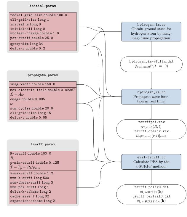
Figure 1: (Color online) The flow chart shows which input parameters (left) are used by which programs (right, light blue). The programs generate output, some of which is read by another program (right, white). This particular example is for the case discussed in Section 4.1, generating the data shown in Figs. 2 and 3.

The range and the resolution of the spectra are determined by the following parameters in tsurff.param: k-max-surff determines the maximum absolute value of momentum, num-k-surff the number of $k$ values for which probabilities are calculated. Setting the parameter delta-k-scheme to 1 samples equidistantly in $k$, 2 equidistantly in energy $\epsilon=k^{2}/2$. num-theta-surff and num-phi-surff define the numbers $N_{\theta_{k}}$, $N_{\varphi_{k}}$ of angles $\theta_{k}$ and $\varphi_{k}$. The values for the angles are distributed equidistantly in the intervals $\theta_{k}\in[0,\pi]$ and $\varphi_{k}\in[0,2\pi)$ (note that if $N_{\theta_{k}}<3$ it is increased to $3$, and if $N_{\theta_{k}}$ is chosen even it is increased by one; in that way $\theta_{k}=0,\pi/2,\pi$ are always covered).

The calculation of a spectrum may be easily parallelized by assigning to each process a part of the $k$ interval. Open MPI [22] is used in the current implementation.

The GNU Scientific Library (GSL) [23] is used for the evaluation of spherical harmonics, Bessel functions, and Wigner $3j$ symbols. The latter are related to the Clebsch-Gordan coefficients appearing in (32) and (35) [21].

Table 2: Comparison of features in Qprop and Qprop 2.0

	Qprop	Qprop 2.0
PES methods	WOM	t-SURFF and WOM
TDDFT capabilities	yes	not yet
length gauge	yes	no
parallel processing	no	yes (PES with t-SURFF)
representation of potentials	plain functions	std::function
parsing parameter files	xml-like format	name-type-value tuples in text file

4 Examples

Four examples for Qprop 2.0 with t-SURFF are provided in the sub-directories ati-tsurff, ati-winop, large-clubs, attoclock, and pow-8-sine. Instructions on how to build and run the sample programs and how to plot the results are detailed in the readme.txt files provided in these directories.

Simulation parameters are read from the text files initial.param, propagate.param and tsurff.param by the programs for imaginary-time propagation, real-time propagation, and the calculation of PES. The flow chart in Fig. 1 visualizes this for the first example in Section 4.1: the parameter files (left) are read by the programs (right) as indicated by lines. Note that both hydrogen_re.cc and eval-tsurff.cc use parameters from all three parameter files.

Some of the output by one program is read by another, e.g., the ground state wavefunction after imaginary-time propagation in hydrogen_im-wf_fin.dat or the wavefunction on the t-SURFF boundary during real time in tsurffpsi.raw. The PES data are finally in the files tsurff-polar0.dat and tsurff-partial0.dat, to be processed by some plot program. In the examples directories gnuplot scripts are provided.

The binding potential $V_{\text{bind}}(r)$, vector potential $\mathbf{A}(t)$, excursion $\bm{\alpha}(t)$, and the imaginary potential $-\mathrm{i}V_{\text{Im}}(r)$ for absorbing outgoing electron flux (that already passed the t-SURFF boundary) are defined in the header file potentials.hh. In all examples the imaginary potential is chosen

$$V_{\text{Im}}(r)=\begin{cases}0&r<R_{\text{Im}}\\ V_{\text{Im,max}}{\left(\frac{r-R_{\text{Im}}}{W_{\text{Im}}}\right)}^{16}&r\geq R_{\text{Im}}\\ \end{cases}$$ (37)

with $V_{\text{Im,max}}=100$, $R_{\text{Im}}=R_{\text{grid}}-W_{\text{Im}}$, and the width of the absorbing region $W_{\text{Im}}$ specified via the parameter imag-width in propagate.param.

An advanced method for the absorption of wavefunctions at grid boundaries with impressively few additional grid points was proposed [24] and could be implemented in a future version of Qprop.

4.1 Window operator vs. t-SURFF

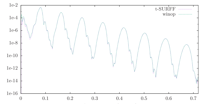
Figure 2: (Color online) Energy-resolved total PES for hydrogen (starting from the 1s state) calculated with t-SURFF and WOM. Laser parameters: $\lambda=535$ nm, $I=2\times 10^{13}\text{ W/cm}^{2}$, $n_{\text{c}}=20$.

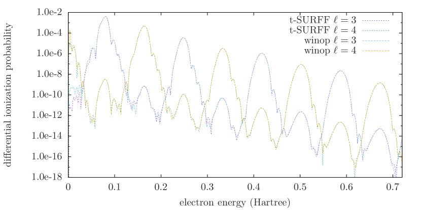
Figure 3: (Color online) Contributions from the $\ell=3$ and $\ell=4$ partial waves to the energy-differential spectrum.

In the first example we show that PES calculated by the t-SURFF approximation are in good agreement with spectra calculated using WOM. All relevant files are located in the directories ati-tsurff and ati-winop, respectively.

In order to ensure that the binding potential vanishes before the t-SURFF boundary a modified Coulomb potential

$$V_{\text{bind}}(r)=\begin{cases}\displaystyle-\frac{1}{r}&\text{if }r<R_{\text{co}}\\ \displaystyle\frac{r-R_{\text{co}}}{R_{\text{co}}^{2}}-\frac{1}{R_{\text{co}}}&\text{if }R_{\text{co}}\leq r<2R_{\text{co}}\\ 0&r\geq 2R_{\text{co}}\end{cases}$$ (38)

with $R_{\text{co}}=25$ (parameter pot-cutoff in initial.param) is used. The t-SURFF boundary is at ${R_{\text{I}}}=100=4R_{\text{co}}$ (parameter R-tsurff) to ensure that even highly-excited bound states are negligible for $r>{R_{\text{I}}}$.

A linearly polarized $n_{\mathrm{c}}=20$-cycle laser pulse described by the vector potential

$$\mathbf{A}(t)=\mathbf{e}_{z}A_{z}(t);\quad A_{z}(t)=\hat{A}\sin^{2}\left(\frac{\omega t}{2n_{\text{c}}}\right)\sin(\omega t+\varphi_{\mathrm{CEP}})$$ (39)

with $\omega=0.085$ (wavelength $\lambda=535$ nm), electric field amplitude $\hat{E}=\hat{A}\omega=0.02387$ (peak intensity $I=2\times 10^{13}\text{ W/cm}^{2}$), and carrier-envelope-phase $\varphi_{\mathrm{CEP}}=0$ is considered.

For this first example we provide step-by-step directions.

1. Switch to the directory qprop-with-tsurff/src/ati-tsurff. You may give a look to readme.txt, Makefile, and the *.param files.

2. Type make (or first make clean and then make).

3. Run the imaginary-time propagation by entering ./hydrogen_im. The ground state is quickly reached within the 5000 imaginary-time steps (specified in hydrogen_im.cc). The executable hydrogen_im generates some output files: the initial wavefunction is stored in hydrogen_im-wf_ini.dat (real and imaginary part in column 1 and 2, respectively), the final wavefunction in hydrogen_im-wf_fin.dat, some observables in hydrogen_im-observ.dat, and grid parameters in hydrogen_im-0.log.

4. Run the real-time propagation by entering ./hydrogen_re. The total number of real time steps 45568 is determined automatically from the sum long( $N_{T_{\mathrm{p}}}+N_{\mathrm{t-SURFF}}+1$) of the pulse duration (in time steps)

   $$N_{T_{\mathrm{p}}}=\frac{n_{\mathrm{c}}\,2\pi/\omega}{\Delta t}=29567.931$$

   and the time

   $$N_{\mathrm{t-SURFF}}=\frac{{R_{\text{I}}}/p_{\min}}{\Delta t}=16000.0$$

   the slowest electron of interest (with momentum $p_{\min}$, assigned to p-min-tsurff in tsurff.param) takes to arrive at ${R_{\text{I}}}$ so that it will be captured for the t-SURFF PES. The real-time propagation takes less than 4 min. on our Intel Core i5-3570 desktop computer. The output file hydrogen_re-vpot_z.dat contains the vector potential $A_{z}(t)$ (2nd column) vs time (1st column), the log-file hydrogen_re.log grid, time, and laser parameters. The file hydrogen_re-obser.dat contains time, the instantaneous energy expectation value $\langle\Psi(t)|\hat{T}+V_{\mathrm{bind}}(r)|\Psi(t)\rangle$ (where $\hat{T}$ is the kinetic energy), the projection on the initial state $|\langle\Psi(0)|\Psi(t)\rangle|^{2}$, the total norm on the grid (drops below unity because of the absorbing potential), and the position expectation value $\langle z\rangle=\langle\Psi(t)|\hat{z}|\Psi(t)\rangle$. Initial and final wavefunction are stored in hydrogen_re-wf.dat as described in the original Qprop paper [1]. The values $1-$total norm on the grid after the simulation and $1-|\langle\Psi(0)|\Psi(t_{\mathrm{final}})\rangle|^{2}$ are stored in hydrogen_re-yield.dat. The relevant output files for the subsequent t-SURFF post-processing are tsurffpsi.raw and tsurff-dpsidr.raw, containing the partial radial wavefunctions and their derivative at $r={R_{\text{I}}}$, respectively.

5. Run the t-SURFF analysis by entering ./eval-tsurff. The wall-clock run time should be less than 3 minutes on a state-of-the-art desktop PC. The spectra are stored in tsurff-partial0.dat and tsurff-polar0.dat. In this example, we focus on the total energy spectrum (36) and the partial contributions $\sqrt{2\epsilon}\big{|}{\bar{a}}_{\text{I, t-SURFF},\ell m}(\sqrt{2\epsilon})\big{|}^{2}$ to it so that only tsurff-partial0.dat is needed. The columns in this file contain (in the case of linear polarization) energy $\epsilon$, momentum $k=\sqrt{2\epsilon}$, partial contributions $k\big{|}{\bar{a}}_{\text{I, t-SURFF},\ell=0,m_{0}}(k)\big{|}^{2},\ldots,k\big{|}{\bar{a}}_{\text{I, t-SURFF},\ell=L_{\max}-1,m_{0}}(k)\big{|}^{2}$, total spectrum ${\mathrm{d}P_{\text{I, t-SURFF}}(\epsilon)}/{\mathrm{d}\epsilon}$. Hence, energy is in column 1 and the total spectrum in column $L_{\max}+3$.

   The t-SURFF analysis may be executed in parallel, as explained in readme.txt.

6. The gnuplot script plot-total-spectrum.gp generates the graphics file total-spectrum.png containing the total t-SURFF PES shown in Fig. 2. For comparison, the script also includes the WOM result (to be calculated next), if present.

7. The gnuplot script plot-partial-spectra.gp generates partial-spectrum.png with the partial t-SURFF PES for $\ell=3$ and $4$, shown in Fig. 3. Again, the script includes the analogous WOM results, if present.

Now we generate the corresponding results using WOM.

1. Switch to the directory qprop-with-tsurff/src/ati-winop. The parameter file initial.param is identical to the one for t-SURFF. However, in propagate.param the radial grid size for real-time propagation is now explicitly specified (R-max double 4000.0, total radial grid size R-max$+$imag-width) whereas in t-SURFF it is calculated automatically as imag-width$+{R_{\text{I}}}+\hat{E}/\omega^{2}$ (which is only 253 for this example). There is another parameter file, winop.param, discussed below.

2. Type make (or first make clean and then make).

3. Run the imaginary-time propagation by entering ./hydrogen_im.

4. Run the real-time propagation by entering ./hydrogen_re. The run time is much longer now ($\simeq$ 38 min. on our desktop computers) because of the by a factor 16 bigger grid, which more than obliterates the advantage due to the smaller number of real time steps long( $N_{T_{\mathrm{p}}}+1$)$=29568$. The hydrogen_re*.dat output files are structured as in ati-tsurff. For instance, in hydrogen_re-obser.dat, column 4, it is seen that the norm on the larger grid stays unity now whereas in ati-tsurff it drops down because the part of the wavefunction representing ionization is absorbed soon after it passed the t-SURFF boundary.

5. Run the WOM analysis by entering ./winop (takes less than 3 minutes). The parameters in winop.param determine that the PES are calculated for num-energy values between energy-min and energy-max. Moreover, more radial grid points may be used for the WOM analysis in order to have a better representation of the continuum (parameter winop-radial-grid-size is set to 50000 in the example). If the radial grid for WOM is too small discrete, “spherical box” states are visible. The result in spectrum_0.dat has the same structure as tsurff-partial0.dat above.

6. The WOM PES are included in the output generated by the gnuplot scripts plot-total-spectrum.gp and plot-partial-spectra.gp in directory ati-tsurff, i.e., Figs. 2 and 3.

Figure 2 shows the energy-resolved spectra for electron emission calculated by the t-SURFF and window operator method respectively. The normalized WOM result and the corresponding $|{\bar{a}}_{\text{I, t-SURFF}}(k)|^{2}k$ with $k=\sqrt{2E}$ from t-SURFF are plotted. The agreement is very good; the results only differ for low energies, as expected.

Both with WOM and t-SURFF the contributions of partial waves of angular momentum index $\ell$ to the energy-differential ionization probability can be computed. Figure 3 shows a comparison of $\big{|}{\bar{a}}_{\text{I, t-SURFF},\ell 0}(k)\big{|}^{2}k|_{k=\sqrt{2\epsilon}}$ calculated by t-SURFF and $\big{|}a_{\text{winop},\ell 0}(\epsilon)\big{|}^{2}$ from WOM (see (36) and (8), respectively) for the partial contributions $\ell=3$ and $\ell=4$.

4.2 Ionization of hydrogen in a strong linearly polarized laser field

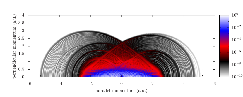
Figure 4: (Color online) Momentum-resolved electron spectrum. Laser parameters: $\lambda=2000$ nm, $I=10^{14}\text{ W/cm}^{2}$, $n_{\text{c}}=6$. A bigger number of angles $N_{\theta_{k}}=400$ and an extended additional propagation time $T_{\text{t-SURFF}}=2000$ than in the example were used to produce the data for this high-resolution PES.

In this example, the momentum-resolved PES shown in Fig. 4 for a hydrogen atom is calculated for laser parameters which make the numerical simulations much more demanding than in the previous example. This example is found in the directory large-clubs.

The binding potential (38) with the cut off radius $R_{\text{co}}=100$ is used. The ground state is obtained after typing make and running ./hydrogem_im, as in the previous example. Entering ./hydrogen_re starts the real-time propagation, simulating the interaction with a linearly polarized $n_{\text{c}}=6$-cycle laser pulse of wavelength $\lambda=2000$ nm, intensity $I=10^{14}\text{ W/cm}^{2}$, and shape (39). It takes about 5 hours on our desktop computer. A rough, conservative estimate for the maximal, relevant orbital angular momentum quantum number is $L_{\max}\simeq(I_{\text{p}}+10U_{\text{p}})/\omega\simeq 623$ where $I_{\text{p}}=0.5$ is the ionization potential and $U_{\text{p}}=\hat{A}^{2}/4\simeq 1.37$ is the ponderomotive potential. The distance of the t-SURFF boundary ${R_{\text{I}}}$ should be larger than the classical quiver amplitude $\hat{A}/\omega\simeq 103$ of a free electron in that laser field. Additionally, wavefunctions of high-lying bound states should be negligible beyond ${R_{\text{I}}}$, which is ensured if ${R_{\text{I}}}$ (here 300) is sufficiently larger than $R_{\text{co}}$ (here 100). The smallest momentum of interest p-min-tsurff, determining the post-laser propagation time as explained in the first example, is chosen 0.5. If one is interested in lower-energy regions (to see the low energy structures, for instance [3]) one should use a smaller value for p-min-surff. It may be more efficient to use WOM instead of tuning p-min-tsurff down to tiny values.

Next, the momentum-resolved PES calculated by the absolute square of (21) is calculated by executing ./eval-tsurff (or the parallel version, see readme.txt). In the interest of a shorter execution time (still 12.4 hours though), a smaller number of angles, a larger p-min-tsurff and a larger grid spacing are used than for the PES shown in Fig. 4.

The gnuplot script plot-polar-spectrum.gp plots the momentum-resolved PES in the $p_{z}p_{x}$-plane from the momentum-angle (i.e., $k$, $\theta_{k}$) data. The high-resolution PES in Fig. 4 beautifully shows many of the textbook features of a strong-field PES in the tunneling regime (the Keldysh parameter is $\gamma=\sqrt{I_{\text{p}}/2U_{\text{p}}}\simeq 0.43<1$): the typical club structure caused by electron rescattering, “holographic side lobes” [2], and intra-cycle interference [25]. Arrows indicate the $p_{\text{max}}=\sqrt{2\times 10U_{\text{p}}}\simeq 5.2$ cutoff for rescattered electrons along the polarization axis. However, because of the short pulse duration different rescattering clubs belonging to different half laser cycles are visible.

Assume we wanted to obtain the same spectrum with WOM. A conservative estimate for the radial grid size is $R_{\text{winop}}=p_{\text{max}}T_{\text{p}}/2\simeq 4328$. With t-SURFF we have only $R_{\text{t-SURFF}}\simeq 550$. The advantage of t-SURFF is even more pronounced for simulations of more laser cycles because the computational cost for propagation scales $\sim T_{\text{p}}^{2}$ for WOM but only $\sim T_{\text{p}}$ for t-SURFF.

4.3 Hydrogen in a circularly polarized laser field

We consider ionization by a circularly polarized laser pulse

$$\mathbf{A}(t)=\mathbf{e}_{x}A_{x}(t)+\mathbf{e}_{y}A_{y}(t),\quad A_{x}(t)=\hat{A}\sin^{2}\left(\frac{\omega t}{2n_{\text{c}}}\right)\sin\omega t,\quad A_{y}(t)=\hat{A}\sin^{2}\left(\frac{\omega t}{2n_{\text{c}}}\right)\cos\omega t.$$ (40)

In a circularly polarized few-cycle laser pulse the ionization time is mapped to the electron’s angle of escape, constituting a so-called “attoclock” [26], which is also the name of the corresponding directory.

We choose $n_{\text{c}}=2$, $\omega=0.114$ (i.e., $\lambda=400$ nm), $\hat{E}=\omega\hat{A}=0.0533799$ (i.e., $I=10^{14}\text{ W/cm}^{2}$) in propagate.param. The binding potential (38) with the cutoff $R_{\text{co}}=25$ is used (see initial.param).

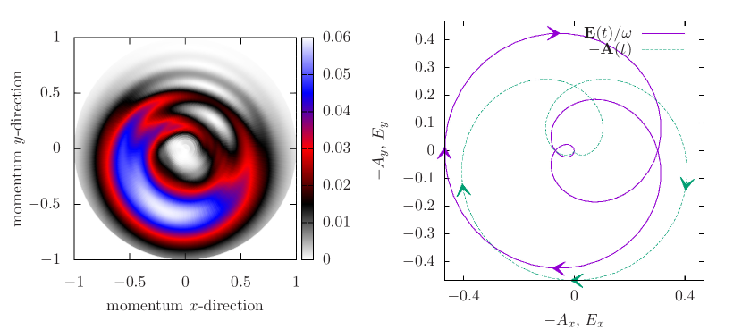
Figure 5: (Color online) Left: Momentum-resolved “attoclock” PES $k\left|a_{\text{I, t-SURFF}}(\mathbf{k})\right|^{2}$ for a two-cycle, circularly polarized laser pulse. Laser parameters: $\lambda=400$ nm, $I=10^{14}\text{ W/cm}^{2}$. Right: Electric field and (negative) vector potential.

As in the previous examples, after the generation of the ground state via running ./hydrogen_im the real-time propagation is started by entering ./hydrogen_re. On our desktop computer this takes 75 minutes. In the file hydrogen_re-obser.dat the columns contain time, field-free energy expectation value $\langle H_{0}\rangle$, projection on initial state, norm on the grid, and the position expectation values $\langle x\rangle$ and $\langle y\rangle$.

PES are calculated with ./eval-tsurff (or mpirun -np $n$ eval-tsurff-mpi for $n$ processes using MPI, see readme.txt). The number of $\theta_{k}$ angles $N_{\theta_{k}}$ and the number of $\varphi_{k}$ angles $N_{\varphi_{k}}$ are defined in tsurff.param. Here, in the attoclock example we set $N_{\theta_{k}}=3$ and $N_{\varphi_{k}}=50$. The run time for ./eval-tsurff is 4.4 hours (and correspondingly faster when processed in parallel). For circular or elliptical polarization in the $xy$-plane the momentum-resolved PES in the $p_{x}p_{y}$-plane is most interesting (unless the wavefunction has a nodal plane there). To that end, the bash shell script select-theta.sh selects the data for $\theta_{k}=\pi/2$ from the tsurff-polar$i_{\text{p}}$.dat file(s) and stores it in tsurff-polar.dat. Finally, the gnuplot script plot-polar-spectrum.gp plots the PES and generates the graphics file polar-spectrum.png.

Figure 5 shows the PES (albeit for higher $N_{\varphi_{k}}$) whose main features can be explained in simple terms: As the right panel shows, the electric field $\mathbf{E}(t)$ peaks in the middle of the pulse, pointing in negative $x$ direction. This implies that the tunneling exit for the electron is at positive $x$ at that most likely emission time. The final drift of the photoelectron according to “simple man’s theory” (see, e.g., [27, 28]) is given by the negative vector potential at the time of emission, pointing in negative $y$ direction. Hence, if the Coulomb interaction between emitted electron and parent ion was negligible, one would expect a maximum probability in the momentum-resolved PES around $p_{x}=0$ and $p_{y}=-\sqrt{2U_{\text{p}}}$, where $U_{\text{p}}=\hat{A}^{2}/2$ for the vector potential (40). However, the Coulomb attraction affects the trajectory of the escaping electron such that it “swings by” and accumulates a drift $p_{x}<0$, explaining why the maximum rotates clockwise away from this expected position, as seen in the left panel of Fig. 5 [29]. An additional rotation might be due to a finite tunneling time [30]. An interference pattern is observed in the first quadrant of the momentum plane, which is due to the two trajectories leading to the same final drift momentum, i.e., the crossing of the $-\mathbf{A}(t)$ curve in Fig. 5, right, Coulomb-rotated clockwise away from the positive $p_{y}$ axis. TDSE simulations for a similar setup where reported in, e.g., [31, 32, 33]. Qprop in propagation mode 44 was used in [34, 29, 32].

4.4 Changing the pulse shape

An example for a pulse shape different from the $\sin^{2}$-case (39) is given in the directory pow-8-sine. We consider linear polarization, $\mathbf{A}(t)=\mathbf{e}_{z}A_{z}(t)$, with

$$A_{z}(t)=\hat{A}\sin^{8}\left(\frac{\omega t}{2n_{\text{c}}}\right)\sin(\omega t+\varphi_{\mathrm{CEP}}).$$ (41)

The power-of-eight envelope is sometimes preferable to the sine-square because the spectral decomposition of the laser pulse is closer to realistic, experimental circumstances. The other parameters are kept the same as in the ati-tsurff example of Section 4.1.

The only modifications necessary to implement a “new” vector potential are in class vecpot, defined in potentials.hh (in the respective example directory). However, apart from the vector potential pulse shape itself, the corresponding time integral, i.e., the excursion $\alpha(t)$, has to be specified there as well. The latter is needed for the t-SURFF post-processing.

After the usual sequence of running make, ./hydrogen_im, ./hydrogen_re, ./eval-tsurff (a matter of a few minutes), gnuplot plot-total-spectrum.gp and gnuplot plot-partial-spectra.gp generate the spectra analogous to Fig. 2 (total-spectrum.png) and 3 (partial-spectra.png). The ATI peaks have less substructure than for the $\sin^{2}$-envelope. The gnuplot script plot-polar-spectrum.gp produces the momentum-resolved PES in tsurff-mom-res.png. A typical multiphoton, ATI-like pattern is observed.

5 Summary

We incorporated the time-dependent surface flux method (t-SURFF) for the calculation of momentum-resolved photoelectron spectra (PES) into the Qprop package. In that way we facilitate the simulation of momentum-resolved PES up to the fastest relevant electron energies (typically ten times the ponderomotive energy) for laser parameters that were inaccessible with the previous version of Qprop based on the window-operator method. In fact, while t-SURFF gets along with grid sizes of the order of the quiver amplitude, the window operator method requires the full, very delocalized wavefunction at the end of the pulse. Especially for long-wavelengths, high intensities, and many laser cycles t-SURFF is numerically much more efficient than the window operator approach as far as the energetic electrons are concerned. Complementary, the slow electrons (and the bound part of the spectrum) can still be calculated using the window operator since the necessary information is contained in the (non-absorbed) wavefunction on the small grid within the t-SURFF boundary.

Several examples were provided, whose execution should enable users to adapt Qprop to their own problems.

Appendix A

The TDSE for an electron in a binding potential $V(\mathbf{r})$ and coupled to an external vector potential in dipole approximation reads

$$\mathrm{i}\partial_{t}\Psi(\mathbf{r},t)=\left\{\frac{1}{2}\left[\mathbf{p}+\mathbf{A}(t)\right]^{2}+V(\mathbf{r})\right\}\Psi(\mathbf{r},t).$$ (42)

The transformation

$$\Psi(\mathbf{r},t)=\Psi^{\prime}(\mathbf{r},t)\ \mathrm{e}^{-\mathrm{i}\int^{t}\mathrm{d}t^{\prime}A^{2}(t^{\prime})/2}$$ (43)

yields the TDSE

$$\mathrm{i}\partial_{t}\Psi^{\prime}(\mathbf{r},t)=\left\{\frac{\mathbf{p}^{2}}{2}+\mathbf{A}(t)\cdot\mathbf{p}+V(\mathbf{r})\right\}\Psi^{\prime}(\mathbf{r},t)$$ (44)

without the $A^{2}(t)$ term. The corresponding Hamiltonian $\hat{H}={\mathbf{p}^{2}}/{2}+\mathbf{A}(t)\cdot\mathbf{p}+V(\mathbf{r})$, with $\mathbf{p}=-\mathrm{i}\nabla$, is used in (1).

References

References

- [1] D. Bauer, P. Koval, Qprop: A schrödinger-solver for intense laser–atom interaction, Computer physics communications 174 (5) (2006) 396–421.
- [2] Y. Huismans, A. Rouzée, A. Gijsbertsen, J. Jungmann, A. Smolkowska, P. Logman, F. Lepine, C. Cauchy, S. Zamith, T. Marchenko, et al., Time-resolved holography with photoelectrons, Science 331 (6013) (2011) 61–64.
-
[3]
B. Wolter, M. G. Pullen, M. Baudisch, M. Sclafani, M. Hemmer, A. Senftleben,
C. D. Schröter, J. Ullrich, R. Moshammer, J. Biegert,
Strong-field physics
with mid-ir fields, Phys. Rev. X 5 (2015) 021034.
doi:10.1103/PhysRevX.5.021034.
URL http://link.aps.org/doi/10.1103/PhysRevX.5.021034 -
[4]
C. D. Lin, A.-T. Le, Z. Chen, T. Morishita, R. Lucchese,
Strong-field
rescattering physics—self-imaging of a molecule by its own electrons,
Journal of Physics B: Atomic, Molecular and Optical Physics 43 (12) (2010)
122001.
URL http://stacks.iop.org/0953-4075/43/i=12/a=122001 -
[5]
K. J. Schafer, K. C. Kulander,
Energy analysis of
time-dependent wave functions: Application to above-threshold ionization,
Phys. Rev. A 42 (1990) 5794–5797.
doi:10.1103/PhysRevA.42.5794.
URL http://link.aps.org/doi/10.1103/PhysRevA.42.5794 - [6] K. Schafer, The energy analysis of time-dependent numerical wave functions, Computer Physics Communications 63 (1) (1991) 427–434.
- [7] M. D. Feit, J. A. Fleck, Jr., A. Steiger, Solution of the Schroedinger equation by a spectral method, Journal of Computational Physics 47 (1982) 412–433. doi:10.1016/0021-9991(82)90091-2.
-
[8]
B. Feuerstein, U. Thumm, On
the computation of momentum distributions within wavepacket propagation
calculations, Journal of Physics B: Atomic, Molecular and Optical Physics
36 (4) (2003) 707.
URL http://stacks.iop.org/0953-4075/36/i=4/a=305 - [9] L. Tao, A. Scrinzi, Photo-electron momentum spectra from minimal volumes: the time-dependent surface flux method, New Journal of Physics 14 (1) (2012) 013021.
-
[10]
K. Boucke, H. Schmitz, H.-J. Kull,
Radiation conditions
for the time-dependent schrödinger equation: Application to strong-field
photoionization, Phys. Rev. A 56 (1997) 763–771.
doi:10.1103/PhysRevA.56.763.
URL http://link.aps.org/doi/10.1103/PhysRevA.56.763 -
[11]
R. M. Feshchenko, A. V. Popov,
Exact transparent
boundary condition for the three-dimensional schrödinger equation in a
rectangular cuboid computational domain, Phys. Rev. E 88 (2013) 053308.
doi:10.1103/PhysRevE.88.053308.
URL http://link.aps.org/doi/10.1103/PhysRevE.88.053308 -
[12]
S. V. Popruzhenko,
Keldysh theory of
strong field ionization: history, applications, difficulties and
perspectives, Journal of Physics B: Atomic, Molecular and Optical Physics
47 (20) (2014) 204001.
URL http://stacks.iop.org/0953-4075/47/i=20/a=204001 - [13] H. Muller, An efficient propagation scheme for the time-dependent schrödinger equation in the velocity gauge, Laser Phys. 9 (1999) 138–148.
- [14] D. Bauer, Qprop manual I, qprop.pdf, http://www.qprop.de, [Online; accessed 2016-02-03].
- [15] C. A. Ullrich, Time-dependent density-functional theory: concepts and applications, Oxford University Press, 2011.
- [16] U. De Giovannini, D. Varsano, M. A. Marques, H. Appel, E. K. Gross, A. Rubio, Ab initio angle-and energy-resolved photoelectron spectroscopy with time-dependent density-functional theory, Physical Review A 85 (6) (2012) 062515.
-
[17]
E. Cormier, P. Lambropoulos,
Optimal gauge and gauge
invariance in non-perturbative time-dependent calculation of above-threshold
ionization, Journal of Physics B: Atomic, Molecular and Optical Physics
29 (9) (1996) 1667.
URL http://stacks.iop.org/0953-4075/29/i=9/a=013 -
[18]
R. Santra, Why
complex absorbing potentials work: A discrete-variable-representation
perspective, Phys. Rev. A 74 (2006) 034701.
doi:10.1103/PhysRevA.74.034701.
URL http://link.aps.org/doi/10.1103/PhysRevA.74.034701 -
[19]
A. Scrinzi,
Infinite-range
exterior complex scaling as a perfect absorber in time-dependent problems,
Phys. Rev. A 81 (2010) 053845.
doi:10.1103/PhysRevA.81.053845.
URL http://link.aps.org/doi/10.1103/PhysRevA.81.053845 -
[20]
D. M. Wolkow, Über eine klasse
von lösungen der diracschen gleichung, Zeitschrift für Physik 94 (3)
(1935) 250–260.
doi:10.1007/BF01331022.
URL http://dx.doi.org/10.1007/BF01331022 - [21] D. A. Varshalovich, A. N. Moskalev, V. K. Khersonskii, Quantum theory of angular momentum, World Scientific, 1988.
- [22] E. Gabriel, G. E. Fagg, G. Bosilca, T. Angskun, J. J. Dongarra, J. M. Squyres, V. Sahay, P. Kambadur, B. Barrett, A. Lumsdaine, et al., Open mpi: Goals, concept, and design of a next generation mpi implementation, in: Recent Advances in Parallel Virtual Machine and Message Passing Interface, Springer, 2004, pp. 97–104.
- [23] B. Gough, GNU scientific library reference manual, Network Theory Ltd., 2009.
- [24] M. Weinmüller, M. Weinmüller, J. Rohland, A. Scrinzi, Perfect absorption in schrödinger-like problems using non-equidistant complex grids, arXiv preprint arXiv:1509.04947.
-
[25]
D. G. Arbó, K. L. Ishikawa, K. Schiessl, E. Persson, J. Burgdörfer,
Intracycle and
intercycle interferences in above-threshold ionization: The time grating,
Phys. Rev. A 81 (2010) 021403.
doi:10.1103/PhysRevA.81.021403.
URL http://link.aps.org/doi/10.1103/PhysRevA.81.021403 - [26] P. Eckle, M. Smolarski, P. Schlup, J. Biegert, A. Staudte, M. Schöffler, H. G. Muller, R. Dörner, U. Keller, Attosecond angular streaking, Nature Physics 4 (7) (2008) 565–570.
-
[27]
D. B. Milošević, G. G. Paulus, D. Bauer, W. Becker,
Above-threshold
ionization by few-cycle pulses, Journal of Physics B: Atomic, Molecular and
Optical Physics 39 (14) (2006) R203.
URL http://stacks.iop.org/0953-4075/39/i=14/a=R01 - [28] P. Mulser, D. Bauer, High Power Laser-Matter Interaction, Springer, 2010.
-
[29]
S. V. Popruzhenko, G. G. Paulus, D. Bauer,
Coulomb-corrected
quantum trajectories in strong-field ionization, Phys. Rev. A 77 (2008)
053409.
doi:10.1103/PhysRevA.77.053409.
URL http://link.aps.org/doi/10.1103/PhysRevA.77.053409 - [30] P. Eckle, A. Pfeiffer, C. Cirelli, A. Staudte, R. Dörner, H. Muller, M. Büttiker, U. Keller, Attosecond ionization and tunneling delay time measurements in helium, Science 322 (5907) (2008) 1525–1529.
-
[31]
C. P. J. Martiny, M. Abu-samha, L. B. Madsen,
Counterintuitive
angular shifts in the photoelectron momentum distribution for atoms in strong
few-cycle circularly polarized laser pulses, Journal of Physics B: Atomic,
Molecular and Optical Physics 42 (16) (2009) 161001.
URL http://stacks.iop.org/0953-4075/42/i=16/a=161001 -
[32]
Y. Li, P. Lan, H. Xie, M. He, X. Zhu, Q. Zhang, P. Lu,
Nonadiabatic
tunnel ionization in strong circularly polarized laser fields:
counterintuitive angular shifts in the photoelectron momentum distribution,
Opt. Express 23 (22) (2015) 28801–28807.
doi:10.1364/OE.23.028801.
URL http://www.opticsexpress.org/abstract.cfm?URI=oe-23-22-28801 -
[33]
M. Murakami, S.-I. Chu,