Polymorphic Type Inference for Machine Code

Abstract

For many compiled languages, source-level types are erased very early in the compilation process. As a result, further compiler passes may convert type-safe source into type-unsafe machine code. Type-unsafe idioms in the original source and type-unsafe optimizations mean that type information in a stripped binary is essentially nonexistent. The problem of recovering high-level types by performing type inference over stripped machine code is called type reconstruction, and offers a useful capability in support of reverse engineering and decompilation.

In this paper, we motivate and develop a novel type system and algorithm for machine-code type inference. The features of this type system were developed by surveying a wide collection of common source- and machine-code idioms, building a catalog of challenging cases for type reconstruction. We found that these idioms place a sophisticated set of requirements on the type system, inducing features such as recursively-constrained polymorphic types. Many of the features we identify are often seen only in expressive and powerful type systems used by high-level functional languages.

Using these type-system features as a guideline, we have developed Retypd: a novel static type-inference algorithm for machine code that supports recursive types, polymorphism, and subtyping. Retypd yields more accurate inferred types than existing algorithms, while also enabling new capabilities such as reconstruction of pointer const annotations with 98% recall. Retypd can operate on weaker program representations than the current state of the art, removing the need for high-quality points-to information that may be impractical to compute.

Reverse Engineering, Type Systems, Polymorphism, Static Analysis, Binary Analysis, Pushdown Automata

1 Introduction

In this paper we introduce Retypd, a machine-code type-inference tool that finds regular types using pushdown systems. Retypd includes several novel features targeted at improved types for reverse engineering, decompilation, and high-level program analyses. These features include:

• Inference of most-general type schemes (§ 5)

• Inference of recursive structure types (§ 2.1)

• Sound analysis of pointer subtyping (§ 3.3)

• Tracking of customizable, high-level information such as purposes and typedef names (§ 3.5)

• Inference of type qualifiers such as const (§ 6.4)

• No dependence on high-quality points-to data (§ 6)

• More accurate recovery of source-level types (§ 6)

Retypd continues in the tradition of SecondWrite [ElWazeer et al., 2013] and TIE [Lee et al., 2011] by introducing a principled static type-inference algorithm applicable to stripped binaries. Diverging from previous work on machine-code type reconstruction, we use a rich type system that supports polymorphism, mutable references, and recursive types. The principled type-inference phase is followed by a second phase that uses heuristics to “downgrade” the inferred types to human-readable C types before display. By factoring type inference into two phases, we can sequester unsound heuristics and quirks of the C type systems from the sound core of the type-inference engine. This adds a degree of freedom to the design space so that we may leverage a relatively complex type system during type analysis, yet still emit familiar C types for the benefit of the reverse engineer.

Retypd operates on an intermediate representation (IR) recovered by automatically disassembling a binary using GrammaTech’s static analysis tool CodeSurfer® for Binaries [Balakrishnan et al., 2005]. By generating type constraints from a TSL-based abstract interpreter [Lim and Reps, 2013], Retypd can operate uniformly on binaries for any platform supported by CodeSurfer, including x86, x86-64, and ARM.

During the development of Retypd, we carried out an extensive investigation of common machine-code idioms in compiled C and C++ code that create challenges for existing type-inference methods. For each challenging case, we identified requirements for any type system that could correctly type the idiomatic code. The results of this investigation appear in § 2. The type system used by Retypd was specifically designed to satisfy these requirements. These common idioms pushed us into a far richer type system than we had first expected, including features like recursively constrained type schemes that have not previously been applied to machine-code type inference.

Due to space limitations, details of the proofs and algorithms appear in the appendices, which are available in the online version of this paper at arXiv:1603.05495 [Noonan et al., ]. Scripts and data sets used for evaluation also appear there.

2 Challenges

There are many challenges to carrying out type inference on machine code, and many common idioms that lead to sophisticated demands on the feature set of a type system. In this section, we describe several of the challenges seen during the development of Retypd that led to our particular combination of type-system features.

2.1 Optimizations after Type Erasure

Since type erasure typically happens early in the compilation process, many compiler optimizations may take well-typed machine code and produce functionally equivalent but ill-typed results. We found that there were three common optimization techniques that required special care: the use of a variable as a syntactic constant, early returns along error paths, and the re-use of stack slots.

Semi-syntactic constants: Suppose a function with signature void f(int x, char* y) is invoked as f(0, NULL). This will usually be compiled to x86 machine code similar to

⬇

push eax ; y := NULL

push eax ; x := 0

call f

This represents a code-size optimization, since push eax can be encoded in one byte instead of the five bytes needed to push an immediate value (0). We must be careful that the type variables for $x$ and $y$ are not unified; here, eax is being used more like a syntactic constant than a dynamic value that should be typed.

Fortuitous re-use of values: A related situation appears in the common control-flow pattern represented by the snippet of C and the corresponding machine code in § 2.1. Note that on procedure exit, the return value in eax may have come from either the return value of S2T or from the return value of get_S (if NULL). If this situation is not detected, we will see a false relationship between the incompatible return types of get_T and get_S.

   ⬇ T * get_T(void) { S * s = get_S(); if (s == NULL) { return NULL; } T * t = S2T(s); return t; }   ⬇ get_T: call get_S test eax, eax jz local_exit push eax call S2T add esp, 4 local_exit: ret   Figure 1: A common fortuitous re-use of a known value. Re-use of stack slots: If a function uses two variables of the same size in disjoint scopes, there is no need to allocate two separate stack slots for those variables. Often the optimizer will reuse a stack slot from a variable that has dropped out of scope. This is true even if the new variable has a different type. This optimization even applies to the stack slots used to store formal-in parameters, as in § 2.1; once the function’s argument is no longer needed, the optimizer can overwrite it with a local variable of an incompatible type. More generally, we cannot assume that the map from program variables to physical locations is one-to-one. We cannot even make the weaker assumption that the program variables inhabiting a single physical location at different times will all belong to a single type. We handle these issues through a combination of type-system features (subtyping instead of unification) and program analyses (reaching definitions for stack variables and trace partitioning [Mauborgne and Rival, 2005]).    ⬇ #include <stdlib.h> struct LL { struct LL * next; int handle; }; int close_last(struct LL * list) { while (list->next != NULL) { list = list->next; } return close(list->handle); }   ⬇ close_last: push ebp mov ebp,esp sub esp,8 mov edx,dword [ebp+arg_0] jmp loc_8048402 loc_8048400: mov edx,eax loc_8048402: mov eax,dword [edx] test eax,eax jnz loc_8048400 mov eax,dword [edx+4] mov dword [ebp+arg_0],eax leave jmp __thunk_.close   $\displaystyle\forall{F}.\,{(\exists\tau.\mathcal{C})}\!\Rightarrow\!{F}$ $\displaystyle\quad\text{where}\quad\mathcal{C}=$ $\displaystyle F.\mathsf{in_{stack0}}$ $\displaystyle{\;\sqsubseteq\;}\tau$ $\displaystyle\tau.\mathsf{load}.\sigma\mathsf{32@0}$ $\displaystyle{\;\sqsubseteq\;}\tau$ $\displaystyle\tau.\mathsf{load}.\sigma\mathsf{32@4}$ $\displaystyle{\;\sqsubseteq\;}\mathsf{int}\wedge^{\#}\!\mathsf{FileDescriptor}$ $\displaystyle\mathsf{int}\vee^{\#}\!\mathsf{SuccessZ}$ $\displaystyle{\;\sqsubseteq\;}F.\mathsf{out_{eax}}$     ⬇ typedef struct { Struct_0 * field_0; int // #FileDescriptor field_4; } Struct_0; int // #SuccessZ close_last(const Struct_0 *);   Figure 2: Example C code (compiled with gcc 4.5.4 on Linux with flags -m32 -O2), disassembly, type scheme inferred from the machine code, and reconstructed C type. The tags ${}^{\#}\!\mathsf{FileDescriptor}$ and ${}^{\#}\!\mathsf{SuccessZ}$ encode inferred higher-level purposes.

2.2 Polymorphic Functions

We discovered that, although not directly supported by the C type system, most programs define or make use of functions that are effectively polymorphic. The most well-known example is malloc: the return value is expected to be immediately cast to some other type T*. Each call to malloc may be thought of as returning some pointer of a different type. The type of malloc is effectively not $\texttt{size\_t}\to\texttt{void*}$, but rather $\forall\tau.\texttt{size\_t}\to\tau\texttt{*}$. The problem of a polymorphic malloc could be mitigated by treating each call site $p$ as a call to a distinct function malloc_p, each of which may have a distinct return type T_p*. Unfortunately, it is not sufficient to treat a handful of special functions like malloc this way: it is common to see binaries that use user-defined allocators and wrappers to malloc. All of these functions would also need to be accurately identified and duplicated for each callsite. A similar problem exists for functions like free, which is polymorphic in its lone parameter. Even more complex are functions like memcpy, which is polymorphic in its first two parameters and its return type, though the three types are not independent of each other. Furthermore, the polymorphic type signatures $\displaystyle\texttt{malloc}:\forall\tau.\texttt{size\_t}\to\tau\texttt{*}$ $\displaystyle\texttt{free}:\forall\tau.\tau\texttt{*}\to\texttt{void}$ $\displaystyle\texttt{memcpy}:\forall\alpha,\beta.(\beta{\;\sqsubseteq\;}\alpha)\Rightarrow(\alpha\texttt{*}\times\beta\texttt{*}\times\texttt{size\_t})\to\alpha\texttt{*}$ are all strictly more informative to the reverse engineer than the standard C signatures. How else could one know that the void* returned by malloc is not meant to be an opaque handle, but rather should be cast to some other pointer type? In compiled C++ binaries, polymorphic functions are even more common. For example, a class member function must potentially accept both base_t* and derived_t* as types for this. Foster et al. [2006] noted that using bounded polymorphic type schemes for libc functions increased the precision of type-qualifier inference, at the level of source code. To advance the state of the art in machine-code type recovery, we believe it is important to also embrace polymorphic functions as a natural and common feature of machine code. Significant improvements to static type reconstruction—even for monomorphic types—will require the capability to infer polymorphic types of some nontrivial complexity.

2.3 Recursive Types

The relevance of recursive types for decompilation was recently discussed by Schwartz et al. [2013], where lack of a recursive type system for machine code was cited as an important source of imprecision. Since recursive data structures are relatively common, it is desirable that a type-inference scheme for machine code be able to represent and infer recursive types natively.

2.4 Offset and Reinterpreted Pointers

Unlike in source code, there is no syntactic distinction in machine code between a pointer-to-struct and a pointer-to-first-member-of-struct. For example, if $X$ has type struct { char*, FILE*, size_t }* on a 32-bit platform, then it should be possible to infer that $X+4$ can be safely passed to fclose; conversely, if $X+4$ is passed to fclose we may need to infer that $X$ points to a structure that, at offset 4, contains a FILE*. This affects the typing of local structures, as well: a structure on the stack may be manipulated using a pointer to its starting address or by manipulating the members directly, e.g., through the frame pointer. These idioms, along with casts from derived* to base*, fall under the general class of physical [Siff et al., 1999] or non-structural [Palsberg et al., 1997] subtyping. In Retypd, we model these forms of subtyping using type scheme specialization (§ 3.5). Additional hints about the extent of local variables are found using data-delineation analysis [Gopan et al., 2015].

2.5 Disassembly Failures

The problem of producing correct disassembly for stripped binaries is equivalent to the halting problem. As a result, we can never assume that our reconstructed program representation will be perfectly correct. Even sound analyses built on top of an unsound program representation may exhibit inconsistencies and quirks. Thus, we must be careful that incorrect disassembly or analysis results from one part of the binary will not influence the correct type results we may have gathered for the rest of the binary. Type systems that model value assignments as type unifications are vulnerable to over-unification issues caused by bad IR. Since unification is non-local, bad constraints in one part of the binary can degrade all type results. Another instance of this problem arises from the use of register parameters. Although the x86 cdecl calling convention uses the stack for parameter passing, most optimized binaries will include many functions that pass parameters in registers for speed. Often, these functions do not conform to any standard calling convention. Although we work hard to ensure that only true register parameters are reported, conservativeness demands the occasional false positive. Type-reconstruction methods that are based on unification are generally sensitive to precision loss due to false-positive register parameters. A common case is the “push ecx” idiom that reserves space for a single local variable in the stack frame of a function $f$. If ecx is incorrectly viewed as a register parameter of $f$ in a unification-based scheme, whatever type variables are bound to ecx at each callsite to $f$ will be mistakenly unified. In our early experiments, we found these overunifications to be a persistent and hard-to-diagnose source of imprecision. In our early unification-based experiments, mitigation heuristics against overunification quickly ballooned into a disproportionately large and unprincipled component of type analysis. We designed Retypd’s subtype-based constraint system to avoid the need for such ad-hoc prophylactics against overunification.

2.6 Cross-casting and Bit Twiddling

Even at the level of source code, there are already many type-unsafe idioms in common use. Most of these idioms operate by directly manipulating the bit representation of a value, either to encode additional information or to perform computations that are not possible using the type’s usual interface. Some common examples include • hashing values by treating them as untyped bit blocks [tr1, 2007], • stealing unused bits of a pointer for tag information, such as whether a thunk has been evaluated [Marlow et al., 2007], • reducing the storage requirements of a doubly-linked list by xor-combining the next and prev pointers, and • directly manipulating the bit representation of another type, as in the quake3 inverse square root trick [Robertson, 2012]. Because of these type-unsafe idioms, it is important that a type-inference scheme continues to produce useful results even in the presence of apparently contradictory constraints. We handle this situation in three ways: 1. separating the phases of constraint entailment, solving, and consistency checking, 2. modeling types with sketches (§ 3.5) that carry more information than C types, and 3. using unions to combine types with otherwise incompatible capabilities (e.g., $\tau$ is both int-like and pointer-like).

2.7 Incomplete Points-to Information

Degradation of points-to accuracy on large programs has been identified as a source of type-precision loss in other systems [ElWazeer et al., 2013]. Our algorithm can provide high-quality types even in the absence of points-to information. Precision can be further improved by increasing points-to knowledge via machine-code analyses such as VSA [Balakrishnan and Reps, 2004], but good results are already attained with no points-to analysis beyond the simpler problem of tracking the stack pointer.

2.8 Ad-hoc Subtyping

Programs may define an ad-hoc type hierarchy via typedefs. This idiom appears in the Windows API, where a variety of handle types are all defined as typedefs of void*. Some of the handle types are to be used as subtypes of other handles; for example, a GDI handle (HGDI) is a generic handle used to represent any one of the more specific HBRUSH, HPEN, etc. In other cases, a typedef may indicate a supertype, as in LPARAM or DWORD; although these are typedefs of int, they have the intended semantics of a generic 32-bit type, which in different contexts may be used as a pointer, an integer, a flag set, and so on. To accurately track ad-hoc hierarchies requires a type system based around subtyping rather than unification. Models for common API type hierarchies are useful; still better is the ability for the end user to define or adjust the initial type hierarchy at run time. We support this feature by parameterizing the main type representation by an uninterpreted lattice $\Lambda$, as described in § 3.5.

3 The Type System

Table 1: Example field labels (type capabilities) in $\Sigma$. Label Variance Capability $\mathsf{.in}_{L}$ $\ominus$ Function with input in location $L$. $\mathsf{.out}_{L}$ $\oplus$ Function with output in location $L$. $\mathsf{.load}$ $\oplus$ Readable pointer. $\mathsf{.store}$ $\ominus$ Writable pointer. $.\sigma\mathsf{N@k}$ $\oplus$ Has $N$-bit field at offset $k$.   Derived Type Variable Formation $\displaystyle\displaystyle{\hbox{\hskip 15.47096pt\vbox{\hbox{\hskip-15.47095pt\hbox{\hbox{$\displaystyle\displaystyle\alpha{\;\sqsubseteq\;}\beta$}}}\vbox{}}}\over\hbox{\hskip 12.37904pt\vbox{\vbox{}\hbox{\hskip-12.37904pt\hbox{\hbox{$\displaystyle\displaystyle\textsc{Var}\;{\alpha}$}}}}}}$ (T-Left)      $\displaystyle\displaystyle{\hbox{\hskip 39.37776pt\vbox{\hbox{\hskip-39.37776pt\hbox{\hbox{$\displaystyle\displaystyle\alpha{\;\sqsubseteq\;}\beta,\quad\textsc{Var}\;{\alpha.\ell}$}}}\vbox{}}}\over\hbox{\hskip 16.31421pt\vbox{\vbox{}\hbox{\hskip-16.31421pt\hbox{\hbox{$\displaystyle\displaystyle\textsc{Var}\;{\beta.\ell}$}}}}}}$ (T-InheritL) $\displaystyle\displaystyle{\hbox{\hskip 15.47096pt\vbox{\hbox{\hskip-15.47095pt\hbox{\hbox{$\displaystyle\displaystyle\alpha{\;\sqsubseteq\;}\beta$}}}\vbox{}}}\over\hbox{\hskip 12.00867pt\vbox{\vbox{}\hbox{\hskip-12.00865pt\hbox{\hbox{$\displaystyle\displaystyle\textsc{Var}\;{\beta}$}}}}}}$ (T-Right)      $\displaystyle\displaystyle{\hbox{\hskip 39.00739pt\vbox{\hbox{\hskip-39.00737pt\hbox{\hbox{$\displaystyle\displaystyle\alpha{\;\sqsubseteq\;}\beta,\quad\textsc{Var}\;{\beta.\ell}$}}}\vbox{}}}\over\hbox{\hskip 16.6846pt\vbox{\vbox{}\hbox{\hskip-16.68459pt\hbox{\hbox{$\displaystyle\displaystyle\textsc{Var}\;{\alpha.\ell}$}}}}}}$ (T-InheritR) $\displaystyle\displaystyle{\hbox{\hskip 16.6846pt\vbox{\hbox{\hskip-16.68459pt\hbox{\hbox{$\displaystyle\displaystyle\textsc{Var}\;{\alpha.\ell}$}}}\vbox{}}}\over\hbox{\hskip 12.37904pt\vbox{\vbox{}\hbox{\hskip-12.37904pt\hbox{\hbox{$\displaystyle\displaystyle\textsc{Var}\;{\alpha}$}}}}}}$ (T-Prefix)   Subtyping            $\displaystyle\displaystyle{\hbox{\hskip 12.37904pt\vbox{\hbox{\hskip-12.37904pt\hbox{\hbox{$\displaystyle\displaystyle\textsc{Var}\;{\alpha}$}}}\vbox{}}}\over\hbox{\hskip 15.84134pt\vbox{\vbox{}\hbox{\hskip-15.84134pt\hbox{\hbox{$\displaystyle\displaystyle\alpha{\;\sqsubseteq\;}\alpha$}}}}}}$ (S-Refl)     $\displaystyle\displaystyle{\hbox{\hskip 59.97964pt\vbox{\hbox{\hskip-59.97963pt\hbox{\hbox{$\displaystyle\displaystyle\alpha{\;\sqsubseteq\;}\beta,\quad\textsc{Var}\;{\beta.\ell},\quad\langle\ell\rangle=\oplus$}}}\vbox{}}}\over\hbox{\hskip 24.08206pt\vbox{\vbox{}\hbox{\hskip-24.08205pt\hbox{\hbox{$\displaystyle\displaystyle\alpha.\ell{\;\sqsubseteq\;}\beta.\ell$}}}}}}$ (S-Field_⊕) $\displaystyle\displaystyle{\hbox{\hskip 37.55428pt\vbox{\hbox{\hskip-37.55426pt\hbox{\hbox{$\displaystyle\displaystyle\alpha{\;\sqsubseteq\;}\beta,\quad\beta{\;\sqsubseteq\;}\gamma$}}}\vbox{}}}\over\hbox{\hskip 15.23149pt\vbox{\vbox{}\hbox{\hskip-15.23148pt\hbox{\hbox{$\displaystyle\displaystyle\alpha{\;\sqsubseteq\;}\gamma$}}}}}}$ (S-Trans)     $\displaystyle\displaystyle{\hbox{\hskip 59.97964pt\vbox{\hbox{\hskip-59.97963pt\hbox{\hbox{$\displaystyle\displaystyle\alpha{\;\sqsubseteq\;}\beta,\quad\textsc{Var}\;{\beta.\ell},\quad\langle\ell\rangle=\ominus$}}}\vbox{}}}\over\hbox{\hskip 24.08206pt\vbox{\vbox{}\hbox{\hskip-24.08205pt\hbox{\hbox{$\displaystyle\displaystyle\beta.\ell{\;\sqsubseteq\;}\alpha.\ell$}}}}}}$ (S-Field_⊖) $\displaystyle\displaystyle{\hbox{\hskip 54.52202pt\vbox{\hbox{\hskip-54.52202pt\hbox{\hbox{$\displaystyle\displaystyle\textsc{Var}\;{\alpha.\mathsf{load}},\quad\textsc{Var}\;{\alpha.\mathsf{store}}$}}}\vbox{}}}\over\hbox{\hskip 38.38306pt\vbox{\vbox{}\hbox{\hskip-38.38306pt\hbox{\hbox{$\displaystyle\displaystyle\alpha.\mathsf{store}{\;\sqsubseteq\;}\alpha.\mathsf{load}$}}}}}}$ (S-Pointer) Figure 3: Deduction rules for the type system. $\alpha,\beta,\gamma$ represent derived type variables; $\ell$ represents a label in $\Sigma$. The type system used by Retypd is based around the inference of recursively constrained type schemes (§ 3.1). Solutions to constraint sets are modeled by sketches (§ 3.5); the sketch associated to a value consists of a record of capabilities which that value holds, such as whether it can be stored to, called, or accessed at a certain offset. Sketches also include markings drawn from a customizable lattice $(\Lambda,\vee,\wedge,<:)$, used to propagate high-level information such as typedef names and domain-specific purposes during type inference. Retypd also supports recursively constrained type schemes that abstract over the set of types subject to a constraint set $\mathcal{C}$. The language of type constraints used by Retypd is weak enough that for any constraint set $\mathcal{C}$, satisfiability of $\mathcal{C}$ can be reduced (in cubic time) to checking a set of scalar constraints $\kappa_{1}<:\kappa_{2}$, where $\kappa_{i}$ are constants belonging to $\Lambda$. Thanks to the reduction of constraint satisfiability to scalar constraint checking, we can omit expensive satisfiability checks during type inference. Instead, we delay the check until the final stage when internal types are converted to C types for display, providing a natural place to instantiate union types that resolve any inconsistencies. Since compiler optimizations and type-unsafe idioms in the original source frequently lead to program fragments with unsatisfiable type constraints (§ 2.5, § 2.6), this trait is particularly desirable.

3.1 Syntax: the Constraint Type System

Throughout this section, we fix a set $\mathcal{V}$ of type variables, an alphabet $\Sigma$ of field labels, and a function $\langle\cdot\rangle:\Sigma\to\{\oplus,\ominus\}$ denoting the variance (3.2) of each label. We do not require the set $\Sigma$ to be finite. Retypd makes use of a large set of labels; for simplicity, we will focus on those in Table 1. Within $\mathcal{V}$, we assume there is a distinguished set of type constants. These type constants are symbolic representations $\overline{\kappa}$ of elements $\kappa$ belonging to some lattice, but are otherwise uninterpreted. It is usually sufficient to think of the type constants as type names or semantic tags.

Definition 3.1.

A derived type variable is an expression of the form $\alpha w$ with $\alpha\in\mathcal{V}$ and $w\in\Sigma^{*}$.

Definition 3.2.

The variance of a label $\ell$ encodes the subtype relationship between $\alpha.\ell$ and $\beta.\ell$ when $\alpha$ is a subtype of $\beta$, formalized in rules $\textsc{S-Field}_{\oplus}$ and $\textsc{S-Field}_{\ominus}$ of Figure 3. The variance function $\langle\cdot\rangle$ can be extended to $\Sigma^{*}$ by defining $\langle\varepsilon\rangle=\oplus$ and $\langle xw\rangle=\langle x\rangle\cdot\langle w\rangle$, where $\{\oplus,\ominus\}$ is the sign monoid with $\oplus\cdot\oplus=\ominus\cdot\ominus=\oplus$ and $\oplus\cdot\ominus=\ominus\cdot\oplus=\ominus$. A word $w\in\Sigma^{*}$ is called covariant if $\langle w\rangle=\oplus$, or contravariant if $\langle w\rangle=\ominus$.

Definition 3.3.

Let $\mathcal{V}=\{\alpha_{i}\}$ be a set of base type variables. A constraint is an expression of the form $\textsc{Var}\;{X}$ (“existence of the derived type variable $X$”) or $X{\;\sqsubseteq\;}Y$ (“$X$ is a subtype of $Y$”), where $X$ and $Y$ are derived type variables. A constraint set over $\mathcal{V}$ is a finite collection $\mathcal{C}$ of constraints, where the type variables in each constraint are either type constants or members of $\mathcal{V}$. We will say that $\mathcal{C}$ entails $c$, denoted $\mathcal{C}{\;\vdash\;}c$, if $c$ can be derived from the constraints in $\mathcal{C}$ using the deduction rules of Figure 3. We also allow projections: given a constraint set $\mathcal{C}$ with free variable $\tau$, the projection $\exists\tau.\mathcal{C}$ binds $\tau$ as an “internal” variable in the constraint set. See $\tau$ in § 2.1 for an example or, for a more in-depth treatment of constraint projection, see Su et al. [2002]. The field labels used to form derived type variables are meant to represent capabilities of a type. For example, the constraint $\textsc{Var}\;{\alpha.\mathsf{load}}$ means $\alpha$ is a readable pointer, and the derived type variable $\alpha.\mathsf{load}$ represents the type of the memory region obtained by loading from $\alpha$. Let us briefly see how operations in the original program translate to type constraints, using C-like pseudocode for clarity. The full conversion from disassembly to type constraints is described in Appendix A. Value copies: When a value is moved between program variables in an assignment like x := y, we make the conservative assumption that the type of x may be upcast to a supertype of y. We will generate a constraint of the form $Y{\;\sqsubseteq\;}X$. Loads and stores: Suppose that p is a pointer to a 32-bit type, and a value is loaded into x by the assignment x := *p. Then we will generate a constraint of the form $P.\mathsf{load}.\sigma\mathsf{32@0}{\;\sqsubseteq\;}X$. Similarly, a store *q := y results in the constraint $Y{\;\sqsubseteq\;}Q.\mathsf{store}.\sigma\mathsf{32@0}$. In some of the pointer-based examples in this paper we omit the final $.\sigma\mathsf{N@k}$ access after a $.\mathsf{load}$ or $.\mathsf{store}$ to simplify the presentation. Function calls: Suppose the function $f$ is invoked by y := f(x). We will generate the constraints $X{\;\sqsubseteq\;}F.\mathsf{in}$ and $F.\mathsf{out}{\;\sqsubseteq\;}Y$, reflecting the flow of actuals to and from formals. Note that if we define $A.\mathsf{in}=X$ and $A.\mathsf{out}=Y$ then the two constraints are equivalent to $F{\;\sqsubseteq\;}A$ by the rules of Figure 3. This encodes the fact that the called function’s type must be at least as specific as the type used at the callsite. One of the primary goals of our type-inference engine is to associate to each procedure a most-general type scheme.

Definition 3.4.

A type scheme is an expression of the form $\forall{\overline{\alpha}}.\,{\mathcal{C}}\!\Rightarrow\!{\alpha_{1}}$ where $\forall\overline{\alpha}=\forall\alpha_{1}\dots\forall\alpha_{n}$ is quantification over a set of type variables, and $\mathcal{C}$ is a constraint set over $\{\alpha_{i}\}_{i=1..n}$. Type schemes provide a way of encoding the pre- and post-conditions that a function places on the types in its calling context. Without the constraint sets, we would only be able to represent conditions of the form “the input must be a subtype of $X$” and “the output must be a supertype of $Y$”. The constraint set $\mathcal{C}$ can be used to encode more interesting type relations between inputs and outputs, as in the case of memcpy (§ 2.2). For example, a function that returns the second 4-byte element from a struct* may have the type scheme $\forall{\tau}.\,{(\tau.\mathsf{in}.\mathsf{load}.\sigma\mathsf{32@4}{\;\sqsubseteq\;}\tau.\mathsf{out})}\!\Rightarrow\!{\tau}$.

3.2 Deduction Rules

The deduction rules for our type system appear in Figure 3. Most of the rules are self-evident under the interpretation in 3.3, but a few require some additional motivation. $\textsc{S-Field}_{\oplus}$ and $\textsc{S-Field}_{\ominus}$: These rules ensure that field labels act as co- or contra-variant type operators, generating subtype relations between derived type variables from subtype relations between the original variables. T-InheritL and T-InheritR: The rule T-InheritL should be uncontroversial, since a subtype should have all capabilities of its supertype. The rule T-InheritR is more unusual since it moves capabilities in the other direction; taken together, these rules require that two types in a subtype relation must have exactly the same set of capabilities. This is a form of structural typing, ensuring that comparable types have the same shape. Structural typing appears to be at odds with the need to cast more capable objects to less capable ones, as described in § 2.4. Indeed, T-InheritR eliminates the possibility of forgetting capabilities during value assignments. But we still maintain this capability at procedure invocations due to our use of polymorphic type schemes. An explanation of how type-scheme instantiation enables us to forget fields of an object appears in § 3.4, with more details in § E.1.2. These rules ensure that Retypd can perform “iterative variable recovery”; lack of iterative variable recovery was cited by the creators of the Phoenix decompiler [Schwartz et al., 2013] as a common cause of incorrect decompilation when using TIE [Lee et al., 2011] for type recovery. S-Pointer: This rule is a consistency condition ensuring that the type that can be loaded from a pointer is a supertype of the type that can be stored to a pointer. Without this rule, pointers would provide a channel for subverting the type system. An example of how this rule is used in practice appears in § 3.3. The deduction rules of Figure 3 are simple enough that each proof may be reduced to a normal form (see Theorem B.1). An encoding of the normal forms as transition sequences in a modified pushdown system is used to provide a compact representation of the entailment closure $\overline{\mathcal{C}}=\{c~{}|~{}\mathcal{C}{\;\vdash\;}c\}$. The pushdown system modeling $\overline{\mathcal{C}}$ is queried and manipulated to provide most of the interesting type-inference functionality. An outline of this functionality appears in § 5.2.

3.3 Modeling Pointers

To model pointers soundly in the presence of subtyping, we found that our initial naïve approach suffered from unexpected difficulties when combined with subtyping. Following the C type system, it seemed natural to model pointers by introducing an injective unary type constructor $\mathsf{Ptr}$, so that $\mathsf{Ptr}(T)$ is the type of pointers to $T$. In a unification-based type system, this approach works as expected. In the presence of subtyping, a new issue arises. Consider the two programs in § 3.3. Since the type variables $P$ and $Q$ associated to p, q can be seen to be pointers, we can begin by writing $P=\mathsf{Ptr}(\alpha),Q=\mathsf{Ptr}(\beta)$. The first program will generate the constraint set $\mathcal{C}_{1}=\{\mathsf{Ptr}(\beta){\;\sqsubseteq\;}\mathsf{Ptr}(\alpha),$ $X{\;\sqsubseteq\;}\alpha,$ $\beta{\;\sqsubseteq\;}Y\}$ while the second generates $\mathcal{C}_{2}=\{\mathsf{Ptr}(\beta){\;\sqsubseteq\;}\mathsf{Ptr}(\alpha),$ $X{\;\sqsubseteq\;}\beta,$ $\alpha{\;\sqsubseteq\;}Y\}$. Since each program has the effect of copying the value in $x$ to $y$, both constraint sets should satisfy $\mathcal{C}_{i}{\;\vdash\;}X{\;\sqsubseteq\;}Y$. To do this, the pointer subtype constraint must entail some constraint on $\alpha$ and $\beta$, but which one? If we assume that $\mathsf{Ptr}$ is covariant, then $\mathsf{Ptr}(\beta){\;\sqsubseteq\;}\mathsf{Ptr}(\alpha)$ entails $\beta{\;\sqsubseteq\;}\alpha$ and so $\mathcal{C}_{2}{\;\vdash\;}X{\;\sqsubseteq\;}Y$, but $\mathcal{C}_{1}{\not\;\vdash\;}X{\;\sqsubseteq\;}Y$. On the other hand, if we make $\mathsf{Ptr}$ contravariant then $\mathcal{C}_{1}{\;\vdash\;}X{\;\sqsubseteq\;}Y$ but $\mathcal{C}_{2}{\not\;\vdash\;}X{\;\sqsubseteq\;}Y$. It seems that our only recourse is to make subtyping degenerate to type equality under $\mathsf{Ptr}$: we are forced to declare that $\mathsf{Ptr}(\beta){\;\sqsubseteq\;}\mathsf{Ptr}(\alpha){\;\vdash\;}\alpha=\beta$, which of course means that $\mathsf{Ptr}(\beta)=\mathsf{Ptr}(\alpha)$ already. This is a catastrophe for subtyping as used in machine code, since many natural subtype relations are mediated through pointers. For example, the unary $\mathsf{Ptr}$ constructor cannot handle the simplest kind of C++ class subtyping, where a derived class physically extends a base class by appending new member variables. The root cause of the difficulty seems to be in conflating two capabilities that (most) pointers have: the ability to be written through and the ability to be read through. In Retypd, these two capabilities are modeled using different field labels $\mathsf{.store}$ and $\mathsf{.load}$. The $\mathsf{.store}$ label is contravariant, while the $\mathsf{.load}$ label is covariant.    ⬇ f() { p = q; *p = x; y = *q; }   ⬇ g() { p = q; *q = x; y = *p; }   Figure 4: Two programs, each mediating a copy from x to y through a pair of aliased pointers. To see how the separation of pointer capabilities avoids the loss of precision suffered by $\mathsf{Ptr}$, we revisit the two example programs. The first generates the constraint set $$\mathcal{C}^{\prime}_{1}=\left\{Q{\;\sqsubseteq\;}P,\quad X{\;\sqsubseteq\;}P\mathsf{.store},\quad Q\mathsf{.load}{\;\sqsubseteq\;}Y\right\}$$ By rule T-InheritR we may conclude that $Q$ also has a field of type $\mathsf{.store}$. By S-Pointer we can infer that $Q\mathsf{.store}{\;\sqsubseteq\;}Q\mathsf{.load}$. Finally, since $\mathsf{.store}$ is contravariant and $Q{\;\sqsubseteq\;}P$, $\textsc{S-Field}_{\ominus}$ says we also have $P\mathsf{.store}{\;\sqsubseteq\;}Q\mathsf{.store}$. Putting these parts together gives the subtype chain $$X{\;\sqsubseteq\;}P\mathsf{.store}{\;\sqsubseteq\;}Q\mathsf{.store}{\;\sqsubseteq\;}Q\mathsf{.load}{\;\sqsubseteq\;}Y$$ The second program generates the constraint set $$\mathcal{C}^{\prime}_{2}=\left\{Q{\;\sqsubseteq\;}P,\quad X{\;\sqsubseteq\;}Q\mathsf{.store},\quad P\mathsf{.load}{\;\sqsubseteq\;}Y\right\}$$ Since $Q{\;\sqsubseteq\;}P$ and $P$ has a field $\mathsf{.load}$, we conclude that $Q$ has a $\mathsf{.load}$ field as well. Next, S-Pointer requires that $Q\mathsf{.store}{\;\sqsubseteq\;}Q\mathsf{.load}$. Since $\mathsf{.load}$ is covariant, $Q{\;\sqsubseteq\;}P$ implies that $Q\mathsf{.load}{\;\sqsubseteq\;}P\mathsf{.load}$. This gives the subtype chain $$X{\;\sqsubseteq\;}Q\mathsf{.store}{\;\sqsubseteq\;}Q\mathsf{.load}{\;\sqsubseteq\;}P\mathsf{.load}{\;\sqsubseteq\;}Y$$ By splitting out the read- and write-capabilities of a pointer, we can achieve a sound account of pointer subtyping that does not degenerate to type equality. Note the importance of the consistency condition S-Pointer: this rule ensures that writing through a pointer and reading the result cannot subvert the type system. The need for separate handling of read- and write-capabilities in a mutable reference has been rediscovered multiple times. A well-known instance is the covariance of the array type constructor in Java and C#, which can cause runtime type errors if the array is mutated; in these languages, the read capabilities are soundly modeled only by sacrificing soundness for the write capabilities.

3.4 Non-structural Subtyping and T-InheritR

It was noted in § 3.2 that the rule T-InheritR leads to a system with a form of structural typing: any two types in a subtype relation must have the same capabilities. Superficially, this seems problematic for modeling typecasts that forget about fields, such as a cast from derived* to base* when derived* has additional fields (§ 2.4). The missing piece that allows us to effectively forget capabilities is instantiation of callee type schemes at a callsite. To demonstrate how polymorphism enables forgetfulness, consider the example type scheme $\forall{F}.\,{(\exists\tau.\mathcal{C})}\!\Rightarrow\!{F}$ from § 2.1. The function close_last can be invoked by providing any actual-in type $\alpha$, such that $\alpha{\;\sqsubseteq\;}F.\mathsf{in}_{\mathsf{stack}0}$; in particular, $\alpha$ can have more fields than those required by $\mathcal{C}$. We simply select a more capable type for the existentially-quantified type variable $\tau$ in $\mathcal{C}$. In effect, we have used specialization of polymorphic types to model non-structural subtyping idioms, while subtyping is used only to model structural subtyping idioms. This restricts our introduction of non-structural subtypes to points where a type scheme is instantiated, such as at a call site.

3.5 Semantics: the Poset of Sketches

Figure 5: A sketch instantiating the type scheme in § 2.1. The simple type system defined by the deduction rules of Figure 3 defines the syntax of legal derivations in our type system. The constraint solver of § 5.2 is designed to find a simple representation for all conclusions that can be derived from a set of type constraints. Yet there is no notion of what a type is inherent to the deduction rules of Figure 3. We have defined the rules of the game, but not the equipment with which it should be played. We found that introducing C-like entities at the level of constraints or types resulted in too much loss of precision when working with the challenging examples described in § 2. Consequently we developed the notion of a sketch, a kind of regular tree labeled with elements of an auxiliary lattice $\Lambda$. Sketches are related to the recursive types studied by Amadio and Cardelli [1993] and Kozen et al. [1995], but do not depend on a priori knowledge of the ranked alphabet of type constructors.

Definition 3.5.

A sketch is a (possibly infinite) tree $T$ with edges labeled by elements of $\Sigma$ and nodes marked with elements of a lattice $\Lambda$, such that $T$ only has finitely many subtrees up to labeled isomorphism. By collapsing isomorphic subtrees, we can represent sketches as deterministic finite state automata with each state labeled by an element of $\Lambda$. The set of sketches admits a lattice structure, with operations described by Figure 18. The lattice of sketches serves as the model in which we interpret type constraints. The interpretation of the constraint $\textsc{Var}\;{\alpha.u}$ is “the sketch $S_{\alpha}$ admits a path from the root with label sequence $u$”, and $\alpha.u{\;\sqsubseteq\;}\beta.v$ is interpreted as “the sketch obtained from $S_{\alpha}$ by traversing the label sequence $u$ is a subsketch (in the lattice order) of the sketch obtained from $S_{\beta}$ by traversing the sequence $v$.” The main utility of sketches is that they are nearly a free tree model [Pottier and Rémy, 2005] of the constraint language. Any constraint set $\mathcal{C}$ is satisfiable over the lattice of sketches, as long as $\mathcal{C}$ cannot prove an impossible subtype relation in the auxiliary lattice $\Lambda$. In particular, we can always solve the fragment of $\mathcal{C}$ that does not reference constants in $\Lambda$. Stated operationally, we can always recover the tree structure of sketches that potentially solve $\mathcal{C}$. This observation is formalized by the following theorem:

Theorem 3.1.

Suppose that $\mathcal{C}$ is a constraint set over the variables $\{\tau_{i}\}_{i\in I}$. Then there exist sketches $\{S_{i}\}_{i\in I}$, such that $w\in S_{i}$ if and only if $\mathcal{C}{\;\vdash\;}\textsc{Var}\;{\tau_{i}.w}$.

Proof.

The idea is to symmetrize $\sqsubseteq$ using an algorithm that is similar in spirit to Steensgaard’s method of almost-linear-time pointer analysis [Steensgaard, 1996]. Begin by forming a graph with one node $n(\alpha)$ for each derived type variable appearing in $\mathcal{C}$, along with each of its prefixes. Add a labeled edge $n(\alpha)\stackrel{{\scriptstyle\ell}}{{\to}}n(\alpha.\ell)$ for each derived type variable $\alpha.\ell$ to form a graph $G$. Now quotient $G$ by the equivalence relation $\sim$ defined by $n(\alpha)\sim n(\beta)$ if $\alpha{\;\sqsubseteq\;}\beta\in\mathcal{C}$, and $n(\alpha^{\prime})\sim n(\beta^{\prime})$ whenever there are edges $n(\alpha)\stackrel{{\scriptstyle\ell}}{{\to}}n(\alpha^{\prime})$ and $n(\beta)\stackrel{{\scriptstyle\ell^{\prime}}}{{\to}}n(\beta^{\prime})$ in $G$ with $n(\alpha)\sim n(\beta)$ where either $\ell=\ell^{\prime}$ or $\ell=\mathsf{.load}$ and $\ell^{\prime}=\mathsf{.store}$. By construction, there exists a path through $G/\!\!\sim$ with label sequence $u$ starting at the equivalence class of $\tau_{i}$ if and only if $\mathcal{C}{\;\vdash\;}\textsc{Var}\;{\tau_{i}.u}$; the (regular) set of all such paths yields the tree structure of $S_{i}$. ∎ Working out the lattice elements that should label $S_{i}$ is a trickier problem; the basic idea is to use the same automaton $Q$ constructed during constraint simplification (Theorem 5.1) to answer queries about which type constants are upper and lower bounds on a given derived type variable. The full algorithm is listed in § D.4. In Retypd, we use a large auxiliary lattice $\Lambda$ containing hundreds of elements that includes a collection of standard C type names, common typedefs for popular APIs, and user-specified semantic classes such as ${}^{\#}\!\mathsf{FileDescriptor}$ in § 2.1. This lattice helps model ad-hoc subtyping and preserve high-level semantic type names, as discussed in § 2.8. Note. Sketches are just one of many possible models for the deduction rules that could be proposed. A general approach is to fix a poset $(\mathcal{T},<:)$ of types, interpret ${\;\sqsubseteq\;}$ as $<:$, and interpret co- and contra-variant field labels as monotone (resp. antimonotone) functions $\mathcal{T}\to\mathcal{T}$. The separation of syntax from semantics allows for a simple way to parameterize the type-inference engine by a model of types. By choosing a model $(\mathcal{T},\equiv)$ with a symmetric relation $\equiv\;\subseteq\mathcal{T}\times\mathcal{T}$, a unification-based type system similar to SecondWrite [ElWazeer et al., 2013] is generated. On the other hand, by forming a lattice of type intervals and interval inclusion, we would obtain a type system similar to TIE [Lee et al., 2011] that outputs upper and lower bounds on each type variable.

4 Analysis Framework

4.1 IR Reconstruction

Retypd is built on top of GrammaTech’s machine-code-analysis tool CodeSurfer for Binaries. CodeSurfer carries out common program analyses on binaries for multiple CPU architectures, including x86, x86-64, and ARM. CodeSurfer is used to recover a high-level IR from the raw machine code; type constraints are generated directly from this IR, and resolved types are applied back to the IR and become visible to the GUI and later analysis phases. CodeSurfer achieves platform independence through TSL [Lim and Reps, 2013], a language for defining a processor’s concrete semantics in terms of concrete numeric types and mapping types that model flag, register, and memory banks. Interpreters for a given abstract domain are automatically created from the concrete semantics simply by specifying the abstract domain $\mathcal{A}$ and an interpretation of the concrete numeric and mapping types. Retypd uses CodeSurfer’s recovered IR to determine the number and location of inputs and outputs to each procedure, as well as the program’s call graph and per-procedure control-flow graphs. An abstract interpreter then generates sets of type constraints from the concrete TSL instruction semantics. A detailed account of the abstract semantics for constraint generation appears in Appendix A.

4.2 Approach to Type Resolution

After the initial IR is recovered, type inference proceeds in two stages: first, type-constraint sets are generated in a bottom-up fashion over the strongly-connected components of the callgraph. Pre-computed type schemes for externally linked functions may be inserted at this stage. Each constraint set is simplified by eliminating type variables that do not belong to the SCC’s interface; the simplification algorithm is outlined in § 5. Once type schemes are available, the callgraph is traversed bottom-up, assigning sketches to type variables as outlined in § 3.5. During this stage, type schemes are specialized based on the calling contexts of each function. Appendix F lists the full algorithms for constraint simplification (1) and solving (2).

4.3 Translation to C Types

The final phase of type resolution converts the inferred sketches to C types for presentation to the user. Since C types and sketches are not directly comparable, this resolution phase necessarily involves the application of heuristic conversion policies. Restricting the heuristic policies to a single post-inference phase provides us with the flexibility to generate high-quality, human-readable C types while maintaining soundness and generality during type reconstruction.

Example 4.1.

A simple example involves the generation of const annotations on pointers. We decided on a policy that only introduced const annotations on function parameters, by annotating the parameter at location $L$ when the constraint set $\mathcal{C}$ for procedure $p$ satisfies $\mathcal{C}{\;\vdash\;}\textsc{Var}\;{p.\mathsf{in}_{L}.\mathsf{load}}$ and $\mathcal{C}{\not\;\vdash\;}\textsc{Var}\;{p.\mathsf{in}_{L}.\mathsf{store}}$. Retypd appears to be the first machine-code type-inference system to infer const annotations; a comparison of our recovered annotations to the original source code appears in § 6.4.

Example 4.2.

A more complex policy is used to decide between union types and generic types when incompatible scalar constraints must be resolved. Retypd merges comparable scalar constraints to form antichains in $\Lambda$; the elements of these antichains are then used for the resulting C union type.

Example 4.3.

The initial type-simplification stage results in types that are as general as possible. Often, this means that types are found to be more general than is strictly helpful to a (human) observer. A policy is applied that specializes type schemes to the most specific scheme that is compatible with all statically-discovered uses. For example, a C++ object may include a getter function with a highly polymorphic type scheme, since it could operate equally well on any structure with a field of the correct type at the correct offset. But we expect that in every calling context, the getter will be called on a specific object type (or perhaps its derived types). We can specialize the getter’s type by choosing the least polymorphic specialization that is compatible with the observed uses. By specializing the function signature before presenting a final C type to the user, we trade some generality for types that are more likely to match the original source.

5 The Simplification Algorithm

In this section, we sketch an outline of the simplification algorithm at the core of the constraint solver. The complete algorithm appears in Appendix D.

5.1 Inferring a Type Scheme

The goal of the simplification algorithm is to take an inferred type scheme $\forall{\overline{\alpha}}.\,{C}\!\Rightarrow\!{\tau}$ for a procedure and create a smaller constraint set $\mathcal{C}^{\prime}$, such that any constraint on $\tau$ implied by $\mathcal{C}$ is also implied by $\mathcal{C}^{\prime}$. Let $\mathcal{C}$ denote the constraint set generated by abstract interpretation of the procedure being analyzed, and let $\overline{\alpha}$ be the set of free type variables in $\mathcal{C}$. We could already use $\forall{\overline{\alpha}}.\,{\mathcal{C}}\!\Rightarrow\!{\tau}$ as the constraint set in the procedure’s type scheme, since the input and output types used in a valid invocation of f are tautologically those that satisfy $\mathcal{C}$. Yet, as a practical matter, we cannot use the constraint set directly, since this would result in constraint sets with many useless free variables and a high growth rate over nested procedures. Instead, we seek to generate a simplified constraint set $\mathcal{C}^{\prime}$, such that if $c$ is an “interesting” constraint and $\mathcal{C}{\;\vdash\;}c$ then $\mathcal{C}^{\prime}{\;\vdash\;}c$ as well. But what makes a constraint interesting?

Definition 5.1.

For a type variable $\tau$, a constraint is called interesting if it has one of the following forms: • A capability constraint of the form $\textsc{Var}\;{\tau.u}$ • A recursive subtype constraint of the form $\tau.u{\;\sqsubseteq\;}\tau.v$ • A subtype constraint of the form $\tau.u{\;\sqsubseteq\;}\overline{\kappa}$ or $\overline{\kappa}{\;\sqsubseteq\;}\tau.u$ where $\overline{\kappa}$ is a type constant. We will call a constraint set $\mathcal{C}^{\prime}$ a simplification of $\mathcal{C}$ if $\mathcal{C}^{\prime}{\;\vdash\;}c$ for every interesting constraint $c$, such that $\mathcal{C}{\;\vdash\;}c$. Since both $\mathcal{C}$ and $\mathcal{C}^{\prime}$ entail the same set of constraints on $\tau$, it is valid to replace $\mathcal{C}$ with $\mathcal{C}^{\prime}$ in any valid type scheme for $\tau$. Simplification heuristics for set-constraint systems were studied by Fähndrich and Aiken [1996]; our simplification algorithm encompasses all of these heuristics.

5.2 Unconstrained Pushdown Systems

The constraint-simplification algorithm works on a constraint set $\mathcal{C}$ by building a pushdown system $\mathcal{P}_{\mathcal{C}}$ whose transition sequences represent valid derivations of subtyping judgements. We briefly review pushdown systems and some necessary generalizations here.

Definition 5.2.

An unconstrained pushdown system is a triple $\mathcal{P}=(\mathcal{V},\Sigma,\Delta)$ where $\mathcal{V}$ is the set of control locations, $\Sigma$ is the set of stack symbols, and $\Delta\subseteq(\mathcal{V}\times\Sigma^{*})^{2}$ is a (possibly infinite) set of transition rules. We will denote a transition rule by $\langle{X};{u}\rangle\hookrightarrow\langle{Y};{v}\rangle$ where $X,Y\in\mathcal{V}$ and $u,v\in\Sigma^{*}$. We define the set of configurations to be $\mathcal{V}\times\Sigma^{*}$. In a configuration $(p,w)$, $p$ is called the control state and $w$ the stack state. Note that we require neither the set of stack symbols, nor the set of transition rules, to be finite. This freedom is required to model the derivation S-Pointer of Figure 3, which corresponds to an infinite set of transition rules.

Definition 5.3.

An unconstrained pushdown system $\mathcal{P}$ determines a transition relation $\longrightarrow$ on the set of configurations: $(X,w)\longrightarrow(Y,w^{\prime})$ if there is a suffix $s$ and a rule $\langle{X};{u}\rangle\hookrightarrow\langle{Y};{v}\rangle$, such that $w=us$ and $w^{\prime}=vs$. The transitive closure of $\longrightarrow$ is denoted $\stackrel{{\scriptstyle*}}{{\longrightarrow}}$. With this definition, we can state the primary theorem behind our simplification algorithm.

Theorem 5.1.

Let $\mathcal{C}$ be a constraint set and $\mathcal{V}$ a set of base type variables. Define a subset $S_{\mathcal{C}}$ of $(\mathcal{V}\cup\Sigma)^{*}\times(\mathcal{V}\cup\Sigma)^{*}$ by $(Xu,Yv)\in S_{\mathcal{C}}$ if and only if $\mathcal{C}{\;\vdash\;}X.u{\;\sqsubseteq\;}Y.v$. Then $S_{\mathcal{C}}$ is a regular set, and an automaton $Q$ to recognize $S_{\mathcal{C}}$ can be constructed in $O(|\mathcal{C}|^{3})$ time.

Proof.

The basic idea is to treat each $X.u{\;\sqsubseteq\;}Y.v\in\mathcal{C}$ as a transition rule $\langle{X};{u}\rangle\hookrightarrow\langle{Y};{v}\rangle$ in the pushdown system $\mathcal{P}$. In addition, we add control states ${{}^{\#}\textsc{Start}},{{}^{\#}\textsc{End}}$ with transitions $\langle{{{}^{\#}\textsc{Start}}};{X}\rangle\hookrightarrow\langle{X};{\varepsilon}\rangle$ and $\langle{X};{\varepsilon}\rangle\hookrightarrow\langle{{{}^{\#}\textsc{End}}};{X}\rangle$ for each $X\in\mathcal{V}$. For the moment, assume that (1) all labels are covariant, and (2) the rule S-Pointer is ignored. By construction, $({{}^{\#}\textsc{Start}},Xu)\stackrel{{\scriptstyle*}}{{\longrightarrow}}({{}^{\#}\textsc{End}},Yv)$ in $\mathcal{P}$ if and only if $\mathcal{C}{\;\vdash\;}X.u{\;\sqsubseteq\;}Y.v$. A theorem of Büchi Richard Büchi [1964] ensures that for any two control states $A$ and $B$ in a standard (not unconstrained) pushdown system, the set of all pairs $(u,v)$ with $(A,u)\stackrel{{\scriptstyle*}}{{\longrightarrow}}(B,v)$ is a regular language; Caucal [1992] gives a saturation algorithm that constructs an automaton to recognize this language. In the full proof, we add two novelties: first, we support contravariant stack symbols by encoding variance data into the control states and transition rules. The second novelty involves the rule S-Pointer; this rule is problematic since the natural encoding would result in infinitely many transition rules. We extend Caucal’s construction to lazily instantiate all necessary applications of S-Pointer during saturation. For details, see Appendix D. ∎ Since $\mathcal{C}$ will usually entail an infinite number of constraints, this theorem is particularly useful: it tells us that the full set of constraints entailed by $\mathcal{C}$ has a finite encoding by an automaton $Q$. Further manipulations on the constraint closure, such as efficient minimization, can be carried out on $Q$. By restricting the transitions to and from ${{}^{\#}\textsc{Start}}$ and ${{}^{\#}\textsc{End}}$, the same algorithm is used to eliminate type variables, producing the desired constraint simplifications.

5.3 Overall Complexity of Inference

The saturation algorithm used to perform constraint-set simplification and type-scheme construction is, in the worst case, cubic in the number of subtype constraints to simplify. Since some well-known pointer analysis methods also have cubic complexity (such as Andersen [1994]), it is reasonable to wonder if Retypd’s “points-to free” analysis really offers a benefit over a type-inference system built on top of points-to analysis data. To understand where Retypd’s efficiencies are found, first consider the $n$ in $O(n^{3})$. Retypd’s core saturation algorithm is cubic in the number of subtype constraints; due to the simplicity of machine-code instructions, there is roughly one subtype constraint generated per instruction. Furthermore, Retypd applies constraint simplification on each procedure in isolation to eliminate the procedure-local type variables, resulting in constraint sets that only relate procedure formal-ins, formal-outs, globals, and type constants. In practice, these simplified constraint sets are small. Since each procedure’s constraint set is simplified independently, the $n^{3}$ factor is controlled by the largest procedure size, not the overall size of the binary. By contrast, source-code points-to analysis such as Andersen’s are generally cubic in the overall number of pointer variables, with exponential duplication of variables depending on the call-string depth used for context sensitivity. The situation is even more difficult for machine-code points-to analyses such as VSA, since there is no syntactic difference between a scalar and a pointer in machine code. In effect, every program variable must be treated as a potential pointer. On our benchmark suite of real-world programs, we found that execution time for Retypd scales slightly below $O(N^{1.1})$, where $N$ is the number of program instructions. The following back-of-the-envelope calculation can heuristically explain much of the disparity between the $O(N^{3})$ theoretical complexity and the $O(N^{1.1})$ measured complexity. On our benchmark suite, the maximum procedure size $n$ grew roughly like $n\approx N^{2/5}$. We could then expect that a per-procedure analysis would perform worst when the program is partitioned into $N^{3/5}$ procedures of size $N^{2/5}$. On such a program, a per-procedure $O(n^{k})$ analysis may be expected to behave more like an $O(N^{3/5}\cdot(N^{2/5})^{k})=O(N^{({3+2k})/{5}})$ analysis overall. In particular, a per-procedure cubic analysis like Retypd could be expected to scale like a global $O(N^{1.8})$ analysis. The remaining differences in observed versus theoretical execution time can be explained by the facts that real-world constraint graphs do not tend to exercise the simplification algorithm’s worst-case behavior, and that the distribution of procedure sizes is heavily weighted towards small procedures.

6 Evaluation

 

⬇ INT_PTR Proto_EnumAccounts(WPARAM wParam, LPARAM lParam) { *( int* )wParam = accounts.getCount(); *( PROTOACCOUNT*** )lParam = accounts.getArray(); return 0; }

Figure 6: Ground-truth types declared in the original source do not necessarily reflect program semantics. Example from miranda32.

6.1 Implementation

Retypd is implemented as a module within CodeSurfer for Binaries. By leveraging the multi-platform disassembly capabilities of CodeSurfer, it can operate on x86, x86-64, and ARM code. We performed the evaluation using minimal analysis settings, disabling value-set analysis (VSA) but computing affine relations between the stack and frame pointers. Enabling additional CodeSurfer phases such as VSA can greatly improve the reconstructed IR, at the expense of increased analysis time. Existing type-inference algorithms such as TIE [Lee et al., 2011] and SecondWrite [ElWazeer et al., 2013] require some modified form of VSA to resolve points-to data. Our approach shows that high-quality types can be recovered in the absence of points-to information, allowing type inference to proceed even when computing points-to data is too unreliable or expensive.

6.2 Evaluation Setup

Benchmark Description Instructions CodeSurfer benchmarks libidn Domain name translator 7K Tutorial00 Direct3D tutorial 9K zlib Compression library 14K ogg Multimedia library 20K distributor UltraVNC repeater 22K libbz2 BZIP library, as a DLL 37K glut The glut32.dll library 40K pngtest A test of libpng 42K freeglut The freeglut.dll library 77K miranda IRC client 100K XMail Email server 137K yasm Modular assembler 190K python21 Python 2.1 202K quake3 Quake 3 281K TinyCad Computed-aided design 544K Shareaza Peer-to-peer file sharing 842K SPEC2006 benchmarks 470.lbm Lattice Boltzmann Method 3K 429.mcf Vehicle scheduling 3K 462.libquantum Quantum computation 11K 401.bzip2 Compression 13K 458.sjeng Chess AI 25K 433.milc Quantum field theory 28K 482.sphinx3 Speech recognition 43K 456.hmmer Protein sequence analysis 71K 464.h264ref Video compression 113K 445.gobmk GNU Go AI 203K 400.perlbench Perl core 261K 403.gcc C/C++/Fortran compiler 751K Figure 7: Benchmarks used for evaluation. All binaries were compiled from source using optimized release configurations. The SPEC2006 benchmarks were chosen to match the benchmarks used to evaluate SecondWrite [ElWazeer et al., 2013]. Our benchmark suite consists of 160 32-bit x86 binaries for both Linux and Windows, compiled with a variety of gcc and Microsoft Visual C/C++ versions. The benchmark suite includes a mix of executables, static libraries, and DLLs. The suite includes the same coreutils and SPEC2006 benchmarks used to evaluate REWARDS, TIE, and SecondWrite [Lin et al., 2010; Lee et al., 2011; ElWazeer et al., 2013]; additional benchmarks came from a standard suite of real-world programs used for precision and performance testing of CodeSurfer for Binaries. All binaries were built with optimizations enabled and debug information disabled. Ground truth is provided by separate copies of the binaries that have been built with the same settings, but with debug information included (DWARF on Linux, PDB on Windows). We used IdaPro [Hex-Rays, 2015] to read the debug information, which allowed us to use the same scripts for collecting ground-truth types from both DWARF and PDB data. All benchmarks were evaluated on a 2.6 GHz Intel Xeon E5-2670 CPU, running on a single logical core. RAM utilization by CodeSurfer and Retypd combined was capped at 10GB. Our benchmark suite includes the individual binaries in Figure 7 as well as the collections of related binaries shown in Figure 10. We found that programs from a single collection tended to share a large amount of common code, leading to highly correlated benchmark results. For example, even though the coreutils benchmarks include many tools with very disparate purposes, all of the tools make use of a large, common set of statically linked utility routines. Over 80% of the .text section in tail consists of such routines; for yes, the number is over 99%. The common code and specific idioms appearing in coreutils make it a particularly low-variance benchmark suite. In order to avoid over-representing these program collections in our results, we treated these collections as clusters in the data set. For each cluster, we computed the average of each metric over the cluster, then inserted the average as a single data point to the final data set. Because Retypd performs well on many clusters, this averaging procedure tends to reduce our overall precision and conservativeness measurements. Still, we believe that it gives a less biased depiction of the algorithm’s expected real-world behavior than does an average over all benchmarks.

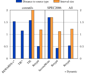
Figure 8: Distance to ground-truth types and size of the interval between inferred upper and lower bounds. Smaller distances represent more accurate types; smaller interval sizes represent increased confidence.

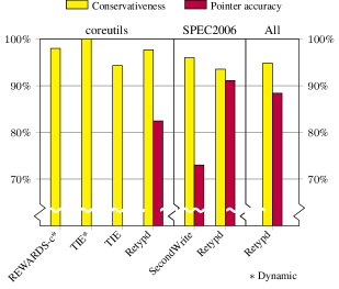
Figure 9: Conservativeness and pointer accuracy metric. Perfect type reconstruction would be 100% conservative and match on 100% of pointer levels. Note that the $y$ axis begins at 70%.

6.3 Sources of Imprecision

Although Retypd is built around a sound core of constraint simplification and solving, there are several ways that imprecision can occur. As described in § 2.5, disassembly failures can lead to unsound constraint generation. Second, the heuristics for converting from sketches to C types are lossy by necessity. Finally, we treat the source types as ground truth, leading to “failures” whenever Retypd recovers an accurate type that does not match the original program—a common situation with type-unsafe source code. A representative example of this last source of imprecision appears in Figure 6. This source code belongs to the miranda32 IRC client, which uses a plugin-based architecture; most of miranda32’s functionality is implemented by “service functions” with the fixed signature int ServiceProc(WPARAM,LPARAM). The types WPARAM and LPARAM are used in certain Windows APIs for generic 16- and 32-bit values. The two parameters are immediately cast to other types in the body of the service functions, as in Figure 6.

6.4 const Correctness

As a side-effect of separately modeling $\mathsf{.load}$ and $\mathsf{.store}$ capabilities, Retypd is easily able to recover information about how pointer parameters are used for input and/or output. We take this into account when converting sketches to C types; if a function’s sketch includes $.\mathsf{in}_{L}.\mathsf{load}$ but not $.\mathsf{in}_{L}.\mathsf{store}$ then we annotate the parameter at $L$ with const, as in Figure 5 and § 2.1. Retypd appears to be the first machine-code type-inference system to infer const annotations directly. On our benchmark suite, we found that 98% of parameter const annotations in the original source code were recovered by Retypd. Furthermore, Retypd inferred const annotations on many other parameters; unfortunately, since most C and C++ code does not use const in every possible situation, we do not have a straightforward way to detect how many of Retypd’s additional const annotations are correct. Manual inspection of the missed const annotations shows that most instances are due to imprecision when analyzing one or two common statically linked library functions. This imprecision then propagates outward to callers, leading to decreased const correctness overall. Still, we believe the 98% recovery rate shows that Retypd offers a useful approach to const inference.

6.5 Comparisons to Other Tools

We gathered results over several metrics that have been used to evaluate SecondWrite, TIE, and REWARDS. These metrics were defined by Lee et al. [2011] and are briefly reviewed here. TIE infers upper and lower bounds on each type variable, with the bounds belonging to a lattice of C-like types. The lattice is naturally stratified into levels, with the distance between two comparable types roughly being the difference between their levels in the lattice, with a maximum distance of 4. A recursive formula for computing distances between pointer and structural types is also used. TIE also determines a policy that selects between the upper and lower bounds on a type variable for the final displayed type. TIE considers three metrics based on this lattice: the conservativeness rate, the interval size, and the distance. A type interval is conservative if the interval bounds overapproximate the declared type of a variable. The interval size is the lattice distance from the upper to the lower bound on a type variable. The distance measures the lattice distance from the final displayed type to the ground-truth type. REWARDS and SecondWrite both use unification-based algorithms, and have been evaluated using the same TIE metrics. The evaluation of REWARDS using TIE metrics appears in Lee et al. [2011]. Distance and interval size: Retypd shows substantial improvements over other approaches in the distance and interval-size metrics, indicating that it generates more accurate types with less uncertainty. The mean distance to the ground-truth type was 0.54 for Retypd, compared to 1.15 for dynamic TIE, 1.53 for REWARDS, 1.58 for static TIE, and 1.70 for SecondWrite. The mean interval size shrunk to 1.2 with Retypd, compared to 1.7 for SecondWrite and 2.0 for TIE. Multi-level pointer accuracy: ElWazeer et al. [2013] also introduced a multi-level pointer-accuracy rate that attempts to quantify how many “levels” of pointers were correctly inferred. On SecondWrite’s benchmark suite, Retypd attained a mean multi-level pointer accuracy of 91%, compared with SecondWrite’s reported 73%. Across all benchmarks, Retypd averages 88% pointer accuracy. Conservativeness: The best type system would have a high conservativeness rate (few unsound decisions) coupled with a low interval size (tightly specified results) and low distance (inferred types are close to ground-truth types). In each of these metrics, Retypd performs about as well or better than existing approaches. Retypd’s mean conservativeness rate is 95%, compared to 94% for TIE. But note that TIE was evaluated only on coreutils; on that cluster, Retypd’s conservativeness was 98%. SecondWrite’s overall conservativeness is 96%, measured on a subset of the SPEC2006 benchmarks; Retypd attained a slightly lower 94% on this subset. It is interesting to note that Retypd’s conservativeness rate on coreutils is comparable to that of REWARDS, even though REWARDS’ use of dynamic execution traces suggests it would be more conservative than a static analysis by virtue of only generating feasible type constraints. Cluster Count Description Instructions Distance Interval Conserv. Ptr. Acc. Const freeglut-demos 3 freeglut samples 2K 0.66 1.49 97% 83% 100% coreutils 107 GNU coreutils 8.23 10K 0.51 1.19 98% 82% 96% vpx-d 8 VP$x$ decoders 36K 0.63 1.68 98% 92% 100% vpx-e 6 VP$x$ encoders 78K 0.63 1.53 96% 90% 100% sphinx2 4 Speech recognition 83K 0.42 1.09 94% 91% 99% putty 4 SSH utilities 97K 0.51 1.05 94% 86% 99% Retypd, as reported 0.54 1.20 95% 88% 98% Retypd, without clustering 0.53 1.22 97% 84% 97% Figure 10: Clusters in the benchmark suite. For each metric, the average over the cluster is given. If a cluster average is worse than Retypd’s overall average for a certain metric, a box is drawn around the entry.

6.6 Performance

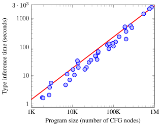
Figure 11: Type-inference time on benchmarks. The line indicates the best-fit exponential $t=0.000725\cdot N^{1.098}$, demonstrating slightly superlinear real-world scaling behavior. The coefficient of determination is $R^{2}=0.977$.

Figure 12: Type-inference memory usage on benchmarks. The line indicates the best-fit exponential $m=0.037\cdot N^{0.846}$, with coefficient of determination $R^{2}=0.959$.

Although the core simplification algorithm of Retypd has cubic worst-case complexity, it only needs to be applied on a per-procedure basis. This suggests that the real-world scaling behavior will depend on the distribution of procedure sizes, not on the whole-program size. In practice, Figure 12 suggests that Retypd gives nearly linear performance over the benchmark suite, which ranges in size from 2K to 840K instructions. To measure Retypd’s performance, we used numerical regression to find the best-fit model $T=\alpha N^{\beta}$ relating execution time $T$ to program size $N$. This results in the relation $T=0.000725\cdot N^{1.098}$ with coefficient of determination $R^{2}=0.977$, suggesting that nearly 98% of the variation in performance data can be explained by this model. In other words, on real-world programs Retypd demonstrates nearly linear scaling of execution time. The cubic worst-case per-procedure behavior of the constraint solver does not translate to cubic behavior overall. Similarly, we found that the sub-linear model $m=0.037\cdot N^{0.846}$ explains 96% of the memory usage in Retypd. Note. The regressions above were performed by numerically fitting exponential models in $(N,T)$ and $(N,m)$ space, rather than analytically fitting linear models in $\log$-$\log$ space. Our models then minimize the error in the predicted values of $T$ and $m$, rather than minimizing errors in $\log T$ or $\log m$. Linear regression in $\log$-$\log$ space results in the less-predicative models $T=0.0003\cdot N^{1.14}$ ($R^{2}=0.92$) and $m=0.08\cdot N^{0.77}$ ($R^{2}=0.88$). The constraint-simplification workload of Retypd would be straightforward to parallelize over the directed acyclic graph of strongly-connected components in the callgraph, further reducing the scaling constant. If a reduction in memory usage is required, Retypd could swap constraint sets to disk; the current implementation keeps all working sets in RAM.

7 Related Work

Machine-code type recovery: Hex-Ray’s reverse engineering tool IdaPro [Hex-Rays, 2015] is an early example of type reconstruction via static analysis. The exact algorithm is proprietary, but it appears that IdaPro propagates types through unification from library functions of known signature, halting the propagation when a type conflict appears. IdaPro’s reconstructed IR is relatively sparse, so the type propagation fails to produce useful information in many common cases, falling back to the default int type. However, the analysis is very fast. SecondWrite [ElWazeer et al., 2013] is an interesting approach to static IR reconstruction with a particular emphasis on scalability. The authors combine a best-effort VSA variant for points-to analysis with a unification-based type-inference engine. Accurate types in SecondWrite depend on high-quality points-to data; the authors note that this can cause type accuracy to suffer on larger programs. In contrast, Retypd is not dependent on points-to data for type recovery and makes use of subtyping rather than unification for increased precision. TIE [Lee et al., 2011] is a static type-reconstruction tool used as part of Carnegie Mellon University’s binary-analysis platform (BAP). TIE was the first machine-code type-inference system to track subtype constraints and explicitly maintain upper and lower bounds on each type variable. As an abstraction of the C type system, TIE’s type lattice is relatively simple; missing features, such as recursive types, were later identified by the authors as an important target for future research [Schwartz et al., 2013]. HOWARD [Slowinska et al., 2011] and REWARDS [Lin et al., 2010] both take a dynamic approach, generating type constraints from execution traces. Through a comparison with HOWARD, the creators of TIE showed that static type analysis can produce higher-precision types than dynamic type analysis, though a small penalty must be paid in conservativeness of constraint-set generation. TIE also showed that type systems designed for static analysis can be easily modified to work on dynamic traces; we expect the same is true for Retypd, though we have not yet performed these experiments. Most previous work on machine-code type recovery, including TIE and SecondWrite, either disallows recursive types or only supports recursive types by combining type-inference results with a points-to oracle. For example, to infer that $x$ has a the type struct S { struct S *, ...}* in a unification-based approach like SecondWrite, first we must have resolved that $x$ points to some memory region $M$, that $M$ admits a 4-byte abstract location $\alpha$ at offset 0, and that the type of $\alpha$ should be unified with the type of $x$. If pointer analysis has failed to compute an explicit memory region pointed to by $x$, it will not be possible to determine the type of $x$ correctly. The complex interplay between type inference, points-to analysis, and abstract-location delineation leads to a relatively fragile method for inferring recursive types. In contrast, our type system can infer recursive types even when points-to facts are completely absent. Robbins et al. [2013] developed an SMT solver equipped with a theory of rational trees and applied it to type reconstruction. Although this allows for recursive types, the lack of subtyping and the performance of the SMT solver make it difficult to scale this approach to real-world binaries. Except for test cases on the order of 500 instructions, precision of the recovered types was not assessed. Related type systems: The type system used by Retypd is related to the recursively constrained types (rc types) of Eifrig, Smith, and Trifonov [1995]. Retypd generalizes the rc type system by building up all types using flexible records; even the function-type constructor $\to$, taken as fundamental in the rc type system, is decomposed into a record with $\mathsf{in}$ and $\mathsf{out}$ fields. This allows Retypd to operate without the knowledge of a fixed signature from which type constructors are drawn, which is essential for analysis of stripped machine code. The use of CFL reachability to perform polymorphic subtyping first appeared in Rehof and Fähndrich [2001], extending previous work relating simpler type systems to graph reachability [Agesen, 1994; Palsberg and O’Keefe, 1995]. Retypd continues by adding type-safe handling of pointers and a simplification algorithm that allows us to compactly represent the type scheme for each function. CFL reachability has also been used to extend the type system of Java [Greenfieldboyce and Foster, 2007] and C++ [Foster et al., 2006] with support for additional type qualifiers. Our reconstructed const annotations can be seen as an instance of this idea, although our qualifier inference is not separated from type inference. To the best of our knowledge, no prior work has applied polymorphic type systems with subtyping to machine code.

8 Future Work

One interesting avenue for future research could come from the application of dependent and higher-rank type systems to machine-code type inference, although we rapidly approach the frontier where type inference is undecidable. A natural example of dependent types appearing in machine code is malloc, which could be typed as ${\verb|malloc|}:(n:{\verb|size_t|})\to\top_{n}$ where $\top_{n}$ denotes the common supertype of all $n$-byte types. The key feature is that the value of a parameter determines the type of the result. Higher-rank types are needed to properly model functions that accept pointers to polymorphic functions as parameters. Such functions are not entirely uncommon; for example, any function that is parameterized by a custom polymorphic allocator will have rank $\geq 2$. Retypd was implemented as an inference phase that runs after CodeSurfer’s main analysis loop. We expect that by moving Retypd into CodeSurfer’s analysis loop, there will be an opportunity for interesting interactions between IR generation and type reconstruction.

9 Conclusion

By examining a diverse corpus of optimized binaries, we have identified a number of common idioms that are stumbling blocks for machine-code type inference. For each of these idioms, we identified a type-system feature that could enable the difficult code to be properly typed. We gathered these features into a type system and implemented the inference algorithm in the tool Retypd. Despite removing the requirement for points-to data, Retypd is able to accurately and conservatively type a wide variety of real-world binaries. We assert that Retypd demonstrates the utility of high-level type systems for reverse engineering and binary analysis.

Acknowledgments

The authors would like to thank Vineeth Kashyap and the anonymous reviewers for their many useful comments on this manuscript, and John Phillips, David Ciarletta, and Tim Clark for their help with test automation.

Appendix A Constraint Generation

Type constraint generation is performed by a parameterized abstract interpretation $\textsc{Type}_{\textsc{A}}$; the parameter A is itself an abstract interpreter that is used to transmit additional analysis information such as reaching definitions, propagated constants, and value-sets (when available). Let $\mathcal{V}$ denote the set of type variables and $\mathcal{C}$ the set of type constraints. Then the primitive TSL value- and map- types for $\textsc{Type}_{\textsc{A}}$ are given by $\displaystyle\mathsf{BASETYPE}_{\textsc{Type}_{\textsc{A}}}$ $\displaystyle=\mathsf{BASETYPE}_{\textsc{A}}\times 2^{\mathcal{V}}\times 2^{\mathcal{C}}$ $\displaystyle\mathsf{MAP[}\alpha,\beta\mathsf{]}_{\textsc{Type}_{\textsc{A}}}$ $\displaystyle=\mathsf{MAP[}\alpha,\beta\mathsf{]}_{\textsc{A}}\times 2^{\mathcal{C}}$ Since type constraint generation is a syntactic, flow-insensitive process, we can regain flow sensitivity by pairing with an abstract semantics that carries a summary of flow-sensitive information. Parameterizing the type abstract interpretation by A allows us to factor out the particular way in which program variables should be abstracted to types (e.g. SSA form, reaching definitions, and so on).

A.1 Register Loads and Stores

The basic reinterpretations proceed by pairing with the abstract interpreter A. For example, ⬇ regUpdate(s, reg, v) = let (v’, t, c) = v (s’, m) = s s’’ = regUpdate(s’, reg, v’) (u, c’) = A(reg, s’’) in ( s’’, m $\cup$ c $\cup$ { t${\;\sqsubseteq\;}$u } )’ where A(reg, s) produces a type variable from the register reg and the A-abstracted register map s’’. Register loads are handled similarly: ⬇ regAccess(reg, s) = let (s’, c) = s (t, c’) = A(reg, s’) in ( regAccess(reg, s’), t, c $\cup$ c’ )’

Example A.1.

Suppose that A represents the concrete semantics for x86 and A(reg, $\cdot$) yields a type variable $(\mathsf{reg},\{\})$ and no additional constraints. Then the x86 expression mov ebx, eax is represented by the TSL expression regUpdate(S, EBX(), regAccess(EAX(), S)), where S is the initial state $(S_{\text{conc}},\mathcal{C})$. After abstract interpretation, $\mathcal{C}$ will become $\mathcal{C}\cup\{\mathsf{eax}{\;\sqsubseteq\;}\mathsf{ebx}\}$. By changing the parametric interpreter A, the generated type constraints may be made more precise.

Example A.2.

We continue with the example of mov ebx, eax above. Suppose that A represents an abstract semantics that is aware of register reaching definitions, and define A(reg, s) by ⬇ A(reg, s) = case reaching-defs(reg, s) of { p } $\rightarrow$ ($\mathsf{reg}_{p}$, {}) defs $\rightarrow$ let t = fresh c = { $\mathsf{reg}_{p}{\;\sqsubseteq\;}\mathsf{t}$ | p $\in$ defs } in (t, c) where reaching-defs yields the set of definitions of reg that are visible from state s. Then $\textsc{Type}_{\textsc{A}}$ at program point $q$ will update the constraint set $\mathcal{C}$ to $$\mathcal{C}\cup\{\mathsf{eax}_{p}{\;\sqsubseteq\;}\mathsf{ebx}_{q}\}$$ if $p$ is the lone reaching definition of EAX. If there are multiple reaching definitions $P$, then the constraint set will become $$\mathcal{C}\cup\{\mathsf{eax}_{p}{\;\sqsubseteq\;}t~{}|~{}p\in P\}\cup\{t{\;\sqsubseteq\;}\mathsf{ebx}_{q}\}$$

A.2 Addition and Subtraction

It is useful to track translations of a value through additions or subtraction of a constant. To that end, we overload the add(x,y) and sub(x,y) operations in the cases where x or y have statically-determined constant values. For example, if INT32(n) is a concrete numeric value then ⬇ let (v’, t, c) = v in ( add(v’, INT32(n)), t.+n, c ) In the case where neither operand is a statically-determined constant, we generate a fresh type variable representing the result and a 3-place constraint on the type variables: ⬇ add(x, y) = let (x’, t₁, c₁) = x (y’, t₂, c₂) = y t = fresh in ( add(x’, y’), t, c₁ $\cup$ c₂ $\cup$ { Add(t₁, t₂, t) } ) Similar interpretations are used for sub(x,y).

A.3 Memory Loads and Stores

Memory accesses are treated similarly to register accesses, except for the use of dereference accesses and the handling of points-to sets. For any abstract A-value a and A-state s, let A(a,s) denote a set of type variables representing the address A in the context s. Furthermore, define $\texttt{PtsTo}_{\textsc{A}}(a,s)$ to be a set of type variables representing the values pointed to by a in the context s. The semantics of the N-bit load and store functions memAccess_N and memUpdate_N are given by ⬇ memAccess${}_{\texttt{N}}$(s, a) = let (s₀, c_s) = s (a₀, t, c_t) = a c_pt = { x${\;\sqsubseteq\;}$t.load.$\sigma$N@0 | x $\in$ PtsTo(a₀,s₀) } in ( memAccess${}_{\texttt{N}}$(s₀, a₀), t.load.$\sigma$N@0, c_s $\cup$ c_t $\cup$ c_pt ) memUpdate${}_{\texttt{N}}$(s, a, v) = let (s₀, c_s) = s (a₀, t, c_t) = a (v₀, v, c_v) = v c_pt = { t.store.$\sigma$N@0${\;\sqsubseteq\;}$x | x $\in$ PtsTo(a₀,s₀) } in ( memUpdate${}_{\texttt{N}}$(s₀, a₀, v₀), c_s $\cup$ c_t $\cup$ c_v $\cup$ c_pt $\cup$ { v${\;\sqsubseteq\;}$t.store.$\sigma$N@0 } ) We achieved acceptable results by using a bare minimum points-to analysis that only tracks constant pointers to the local activation record or the data section. The use of the $\mathsf{.load}$ / $\mathsf{.store}$ accessors allows us to track multi-level pointer information without the need for explicit points-to data. The minimal approach tracks just enough points-to information to resolve references to local and global variables.

A.4 Procedure Invocation

Earlier analysis phases are responsible for delineating procedures and gathering data about each procedure’s formal-in and formal-out variables, including information about how parameters are stored on the stack or in registers. This data is transformed into a collection of locators associated to each function. Each locator is bound to a type variable representing the formal; the locator is responsible for finding an appropriate set of type variables representing the actual at a callsite, or the corresponding local within the procedure itself.

Example A.3.

Consider this simple program that invokes a 32-bit identity function. ⬇ q: call id ... id: ; begin procedure id() r: mov eax, [esp+arg0] ret The procedure id will have two locators: • A locator $L_{i}$ for the single parameter, bound to a type variable $\mathsf{id}_{i}$. • A locator $L_{o}$ for the single return value, bound to a type variable $\mathsf{id}_{o}$. At the procedure call site, the locator $L_{i}$ will return the type variable $\mathsf{ext4}_{p}$ representing the stack location ext4 tagged by its reaching definition. Likewise, $L_{o}$ will return the type variable $\mathsf{eax}_{q}$ to indicate that the actual-out is held in the version of eax that is defined at point $q$. The locator results are combined with the locator’s type variables, resulting in the constraint set $$\{\mathsf{ext4}_{p}{\;\sqsubseteq\;}\mathsf{id}_{i},\quad\mathsf{id}_{o}{\;\sqsubseteq\;}\mathsf{eax}_{q}\}$$ Within procedure id, the locator $L_{i}$ returns the type variable $\mathsf{arg0}_{\verb|id|}$ and $L_{o}$ returns $\mathsf{eax}_{r}$, resulting in the constraint set $$\{\mathsf{id}_{i}{\;\sqsubseteq\;}\mathsf{arg0}_{\verb|id|},\quad\mathsf{eax}_{r}{\;\sqsubseteq\;}\mathsf{id}_{o}\}$$ A procedure may also be associated with a set of type constraints between the locator type variables, called the procedure summary; these type constraints may be inserted at function calls to model the known behavior of a function. For example, invocation of fopen will result in the constraints $$\{\mathsf{fopen}_{i_{0}}{\;\sqsubseteq\;}\underline{\mathsf{char*}},\;\mathsf{fopen}_{i_{1}}{\;\sqsubseteq\;}\underline{\mathsf{char*}},\;\underline{\mathsf{FILE*}}{\;\sqsubseteq\;}\mathsf{fopen}_{o}\}$$ To support polymorphic function invocation, we instantiate fresh versions of the locator type variables that are tagged with the current callsite; this prevents type variables from multiple invocations of the same procedure from being linked.

Example A.4 (cont’d).

When using callsite tagging, the callsite constraints generated by the locators would be $$\{\mathsf{ext4}_{p}{\;\sqsubseteq\;}\mathsf{id}_{i}^{q},\quad\mathsf{id}_{o}^{q}{\;\sqsubseteq\;}\mathsf{eax}_{q}\}$$ The callsite tagging must also be applied to any procedure summary. For example, a call to malloc will result in the constraints $$\{\mathsf{malloc}^{p}_{i}{\;\sqsubseteq\;}\underline{\mathsf{size\_t}},\quad\underline{\mathsf{void*}}{\;\sqsubseteq\;}\mathsf{malloc}^{p}_{o}\}$$ If malloc is used twice within a single procedure, we see an effect like let-polymorphism: each use will be typed independently.

A.5 Other Operations

A.5.1 Floating-point

Floating point types are produced by calls to known library functions and through an abstract interpretation of reads to and writes from the floating point register bank. We do not track register-to-register moves between floating point registers, though it would be straightforward to add this ability. In theory, this causes us to lose precision when attempting to distinguish between typedefs of floating point values; in practice, such typedefs appear to be extremely rare.

A.5.2 Bit Manipulation

We assume that the operands and results of most bit-manipulation operations are integral, with some special exceptions: • Common idioms like xor reg,reg and or reg,-1 are used to initialize registers to certain constants. On x86 these instructions can be encoded with 8-bit immediates, saving space relative to the equivalent versions mov reg,0 and mov reg,-1. We do not assume that the results of these operations are of integral type. • We discard any constraints generated while computing a value that is only used to update a flag status. In particular, on x86 the operation test reg1,reg2 is implemented like a bitwise-and that discards its result, only retaining the effect on the flags. • For specific operations such as $y:=x\textsc{ and }\texttt{0xfffffffc}$ and $y:=x\textsc{ or }1$, we act as if they were equivalent to $y:=x$. This is because these specific operations are often used for bit-stealing; for example, requiring pointers to be aligned on 4-byte boundaries frees the lower two bits of a pointer for other purposes such as marking for garbage collection.

A.6 Additive Constraints

The special constraints Add and Sub are used to conditionally propagate information about which type variables represent pointers and which represent integers when the variables are related through addition or subtraction. The deduction rules for additive constraints are summarized in Figure 13. We obtained good results by inspecting the unification graph used for computing $\mathcal{L}(S_{i})$; the graph can be used to quickly determine whether a variable has pointer- or integer-like capabilities. In practice, the constraint set also should be updated with new subtype constraints as the additive constraints are applied, and a fully applied constraint can be dropped from $\mathcal{C}$. We omit these details for simplicity. Add Sub $X$ $i$ $I$ $p$ $P$ $I$ $i$ $i$ $I$ $P$ $P$ $p$ $p$ $p$ $Y$ $i$ $I$ $I$ $i$ $p$ $P$ $I$ $i$ $i$ $p$ $P$ $i$ $I$ $Z$ $I$ $i$ $P$ $p$ $P$ $p$ $I$ $i$ $p$ $I$ $i$ $P$ $p$ Figure 13: Inference rules for $\textsc{Add}(X,Y;Z)$ and $\textsc{Sub}(X,Y;Z)$. Lower case letters denote known integer or pointer types. Upper case letters denote inferred types. For example, the first column says that if $X$ and $Y$ are integral types in an $\textsc{Add}(X,Y;Z)$ constraint, then $Z$ is integral as well.

Appendix B Normal Forms of Proofs

A finite constraint set with recursive constraints can have an infinite entailment closure. In order to manipulate entailment closures efficiently, we need finite (and small) representations of infinite constraint sets. The first step towards achieving a finite representation of entailment is to find a normal form for every derivation. In Appendix D, finite models of entailment closure will be constructed that manipulate representations of these normal forms.

Lemma B.1.

For any statement $P$ provable from $\mathcal{C}$, there exists a derivation of $\mathcal{C}{\;\vdash\;}P$ that does not use rules S-Refl or T-Inherit.

Proof.

The redundancy of S-Refl is immediate. As for T-Inherit, any use of that rule in a proof can be replaced by $\textsc{S-Field}_{\oplus}$ followed by T-Left, or $\textsc{S-Field}_{\ominus}$ followed by T-Right. ∎ In the following, we make the simplifying assumption that $\mathcal{C}$ is closed under T-Left, T-Right, and T-Prefix. Concretely, we are requiring that 1. if $\mathcal{C}$ contains a subtype constraint $\alpha{\;\sqsubseteq\;}\beta$ as an axiom, it also contains the axioms $\textsc{Var}\;{\alpha}$ and $\textsc{Var}\;{\beta}$. 2. if $\mathcal{C}$ contains a term declaration $\textsc{Var}\;{\alpha}$, it also contains term declarations for all prefixes of $\alpha$.

Lemma B.2.

If $\mathcal{C}$ is closed under T-Left, T-Right, and T-Prefix then any statement provable from $\mathcal{C}$ can be proven without use of T-Prefix.

Proof.

By the previous lemma, we may assume that S-Refl and T-Inherit are not used in the proof. We will prove the lemma by transforming all subproofs that end in a use of T-Prefix to remove that use. To that end, assume we have a proof ending with the derivation of $\textsc{Var}\;{\alpha}$ from $\textsc{Var}\;{\alpha.\ell}$ using T-Prefix. We then enumerate the ways that $\textsc{Var}\;{\alpha.\ell}$ may have been proven. • If $\textsc{Var}\;{\alpha.\ell}\in\mathcal{C}$ then $\textsc{Var}\;{\alpha}\in\mathcal{C}$ already, so the entire proof tree leading to $\textsc{Var}\;{\alpha}$ may be replaced with an axiom from $\mathcal{C}$. • The only other way a $\textsc{Var}\;{\alpha.\ell}$ could be introduced is through T-Left or T-Right. For simplicity, let us only consider the T-Left case; T-Right is similar. At this point, we have a derivation tree that looks like $\displaystyle\displaystyle{\hbox{\hskip 20.21922pt\vbox{\hbox{\hskip-20.21921pt\hbox{\hbox{$\displaystyle\displaystyle\alpha.\ell{\;\sqsubseteq\;}\varphi$}}}\vbox{}}}\over\hbox{\hskip 16.6846pt\vbox{\vbox{}\hbox{\hskip-16.6846pt\hbox{\hbox{$\displaystyle\displaystyle{\hbox{$\displaystyle\displaystyle{\hbox{\hskip 16.6846pt\vbox{\hbox{\hskip-16.68459pt\hbox{\hbox{$\displaystyle\displaystyle\textsc{Var}\;{\alpha.\ell}$}}}\vbox{}}}\over\hbox{\hskip 12.37904pt\vbox{\vbox{}\hbox{\hskip-12.37904pt\hbox{\hbox{$\displaystyle\displaystyle\textsc{Var}\;{\alpha}$}}}}}}$}}$}}}}}}$ How was $\alpha.\ell{\;\sqsubseteq\;}\varphi$ introduced? If it were an axiom of $\mathcal{C}$ then our assumed closure property would imply already that $\textsc{Var}\;{\alpha}\in\mathcal{C}$. The other cases are: – $\varphi=\beta.\ell$ and $\alpha.\ell{\;\sqsubseteq\;}\varphi$ was introduced through one of the S-Field axioms. In either case, $\alpha$ is the left- or right-hand side of one of the antecedents to S-Field, so the whole subderivation including the T-Prefix axiom can be replaced with a single use of T-Left or T-Right. – $\ell=\mathsf{.store}$ and $\varphi=\alpha.\mathsf{load}$, with $\alpha.\ell{\;\sqsubseteq\;}\varphi$ introduced via S-Pointer. In this case, $\textsc{Var}\;{\alpha.\ell}$ is already an antecedent to S-Pointer, so we may elide the subproof up to T-Prefix to inductively reduce the problem to a simpler proof tree. – Finally, we must have $\alpha.\ell{\;\sqsubseteq\;}\varphi$ due to S-Trans. But in this case, the left antecedent is of the form $\alpha.\ell{\;\sqsubseteq\;}\beta$; so once again, we may elide a subproof to get a simpler proof tree. Each of these cases either removes an instance of T-Prefix or results in a strictly smaller proof tree. It follows that iterated application of these simplification rules results in a proof of $\textsc{Var}\;{\alpha}$ with no remaining instances of T-Prefix. ∎

Corollary B.1.

If $\mathcal{C}{\;\vdash\;}\textsc{Var}\;{\alpha}$, then either $\textsc{Var}\;{\alpha}\in\mathcal{C}$, or $\mathcal{C}{\;\vdash\;}\alpha{\;\sqsubseteq\;}\beta,\beta{\;\sqsubseteq\;}\alpha$ for some $\beta$. To simplify the statement of our normal-form theorem, recall that we defined the variadic rule S-Trans’ to remove the degrees of freedom from regrouping repeated application of S-Trans: $\displaystyle\displaystyle{\hbox{\hskip 71.17966pt\vbox{\hbox{\hskip-71.17964pt\hbox{\hbox{$\displaystyle\displaystyle\alpha_{1}{\;\sqsubseteq\;}\alpha_{2},\;\alpha_{2}{\;\sqsubseteq\;}\alpha_{3},\;\dots\;\alpha_{n-1}{\;\sqsubseteq\;}\alpha_{n}$}}}\vbox{}}}\over\hbox{\hskip 18.922pt\vbox{\vbox{}\hbox{\hskip-18.922pt\hbox{\hbox{$\displaystyle\displaystyle\alpha_{1}{\;\sqsubseteq\;}\alpha_{n}$}}}}}}$ (S-Trans’)

Theorem B.1 (Normal form of proof trees).

Let $\mathcal{C}$ be a constraint set that is closed under T-Left, T-Right, and T-Prefix. Then any statement provable from $\mathcal{C}$ has a derivation such that • There are no uses of the rules T-Prefix, T-Inherit, or S-Refl. • For every instance of S-Trans’ and every pair of adjacent antecedents, at least one is not the result of a S-Field application.

Proof.

The previous lemmas already handled the first point. As to the second, suppose that we had two adjacent antecedents that were the result of $\textsc{S-Field}_{\oplus}$: $\displaystyle\displaystyle{\hbox{\hskip 85.22105pt\vbox{\hbox{\hskip-85.22104pt\hbox{\hbox{$\displaystyle\displaystyle\cdots{\hbox{$\displaystyle\displaystyle{\hbox{\hskip 36.78519pt\vbox{\hbox{\hskip-36.78517pt\hbox{\hbox{$\displaystyle\displaystyle{\hbox{$\displaystyle\displaystyle{\hbox{\hskip 3.90453pt\vbox{\hbox{\hskip-3.90451pt\hbox{\hbox{$\displaystyle\displaystyle P$}}}\vbox{}}}\over\hbox{\hskip 15.47096pt\vbox{\vbox{}\hbox{\hskip-15.47095pt\hbox{\hbox{$\displaystyle\displaystyle\alpha{\;\sqsubseteq\;}\beta$}}}}}}$}}\quad{\hbox{$\displaystyle\displaystyle{\hbox{\hskip 3.95277pt\vbox{\hbox{\hskip-3.95277pt\hbox{\hbox{$\displaystyle\displaystyle Q$}}}\vbox{}}}\over\hbox{\hskip 16.31421pt\vbox{\vbox{}\hbox{\hskip-16.31421pt\hbox{\hbox{$\displaystyle\displaystyle\textsc{Var}\;{\beta.\ell}$}}}}}}$}}$}}}\vbox{}}}\over\hbox{\hskip 24.08206pt\vbox{\vbox{}\hbox{\hskip-24.08205pt\hbox{\hbox{$\displaystyle\displaystyle\alpha.\ell{\;\sqsubseteq\;}\beta.\ell$}}}}}}$}}\quad{\hbox{$\displaystyle\displaystyle{\hbox{\hskip 35.93585pt\vbox{\hbox{\hskip-35.93584pt\hbox{\hbox{$\displaystyle\displaystyle{\hbox{$\displaystyle\displaystyle{\hbox{\hskip 3.83508pt\vbox{\hbox{\hskip-3.83507pt\hbox{\hbox{$\displaystyle\displaystyle R$}}}\vbox{}}}\over\hbox{\hskip 14.8611pt\vbox{\vbox{}\hbox{\hskip-14.8611pt\hbox{\hbox{$\displaystyle\displaystyle\beta{\;\sqsubseteq\;}\gamma$}}}}}}$}}\quad{\hbox{$\displaystyle\displaystyle{\hbox{\hskip 3.35416pt\vbox{\hbox{\hskip-3.35416pt\hbox{\hbox{$\displaystyle\displaystyle S$}}}\vbox{}}}\over\hbox{\hskip 16.07474pt\vbox{\vbox{}\hbox{\hskip-16.07474pt\hbox{\hbox{$\displaystyle\displaystyle\textsc{Var}\;{\gamma.\ell}$}}}}}}$}}$}}}\vbox{}}}\over\hbox{\hskip 23.4722pt\vbox{\vbox{}\hbox{\hskip-23.4722pt\hbox{\hbox{$\displaystyle\displaystyle\beta.\ell{\;\sqsubseteq\;}\gamma.\ell$}}}}}}$}}\cdots$}}}\vbox{}}}\over\hbox{\hskip 3.61633pt\vbox{\vbox{}\hbox{\hskip-3.61632pt\hbox{\hbox{$\displaystyle\displaystyle T$}}}}}}$ First, note that the neighboring applications of $\textsc{S-Field}_{\oplus}$ must both use the same field label $\ell$, or else S-Trans would not be applicable. But now observe that we may move a S-Field application upwards, combining the two S-Field applications into one: $\displaystyle\displaystyle{\hbox{\hskip 63.90683pt\vbox{\hbox{\hskip-63.90683pt\hbox{\hbox{$\displaystyle\displaystyle\cdots{\hbox{$\displaystyle\displaystyle{\hbox{\hskip 56.40683pt\vbox{\hbox{\hskip-56.40681pt\hbox{\hbox{$\displaystyle\displaystyle{\hbox{$\displaystyle\displaystyle{\hbox{\hskip 35.33208pt\vbox{\hbox{\hskip-35.33206pt\hbox{\hbox{$\displaystyle\displaystyle{\hbox{$\displaystyle\displaystyle{\hbox{\hskip 3.90453pt\vbox{\hbox{\hskip-3.90451pt\hbox{\hbox{$\displaystyle\displaystyle P$}}}\vbox{}}}\over\hbox{\hskip 15.47096pt\vbox{\vbox{}\hbox{\hskip-15.47095pt\hbox{\hbox{$\displaystyle\displaystyle\alpha{\;\sqsubseteq\;}\beta$}}}}}}$}}\quad{\hbox{$\displaystyle\displaystyle{\hbox{\hskip 3.83508pt\vbox{\hbox{\hskip-3.83507pt\hbox{\hbox{$\displaystyle\displaystyle R$}}}\vbox{}}}\over\hbox{\hskip 14.8611pt\vbox{\vbox{}\hbox{\hskip-14.8611pt\hbox{\hbox{$\displaystyle\displaystyle\beta{\;\sqsubseteq\;}\gamma$}}}}}}$}}$}}}\vbox{}}}\over\hbox{\hskip 15.23149pt\vbox{\vbox{}\hbox{\hskip-15.23148pt\hbox{\hbox{$\displaystyle\displaystyle\alpha{\;\sqsubseteq\;}\gamma$}}}}}}$}}\quad{{\hbox{$\displaystyle\displaystyle{\hbox{\hskip 3.35416pt\vbox{\hbox{\hskip-3.35416pt\hbox{\hbox{$\displaystyle\displaystyle S$}}}\vbox{}}}\over\hbox{\hskip 16.07474pt\vbox{\vbox{}\hbox{\hskip-16.07474pt\hbox{\hbox{$\displaystyle\displaystyle\textsc{Var}\;{\gamma.\ell}$}}}}}}$}}}$}}}\vbox{}}}\over\hbox{\hskip 23.84259pt\vbox{\vbox{}\hbox{\hskip-23.84258pt\hbox{\hbox{$\displaystyle\displaystyle\alpha.\ell{\;\sqsubseteq\;}\gamma.\ell$}}}}}}$}}\cdots$}}}\vbox{}}}\over\hbox{\hskip 3.61633pt\vbox{\vbox{}\hbox{\hskip-3.61632pt\hbox{\hbox{$\displaystyle\displaystyle T$}}}}}}$ For completeness, we also compute the simplifying transformation for adjacent uses of $\textsc{S-Field}_{\ominus}$: the derivation $\displaystyle\displaystyle{\hbox{\hskip 85.83092pt\vbox{\hbox{\hskip-85.8309pt\hbox{\hbox{$\displaystyle\displaystyle\cdots{\hbox{$\displaystyle\displaystyle{\hbox{\hskip 37.15558pt\vbox{\hbox{\hskip-37.15556pt\hbox{\hbox{$\displaystyle\displaystyle{\hbox{$\displaystyle\displaystyle{\hbox{\hskip 3.90453pt\vbox{\hbox{\hskip-3.90451pt\hbox{\hbox{$\displaystyle\displaystyle P$}}}\vbox{}}}\over\hbox{\hskip 15.47096pt\vbox{\vbox{}\hbox{\hskip-15.47095pt\hbox{\hbox{$\displaystyle\displaystyle\beta{\;\sqsubseteq\;}\alpha$}}}}}}$}}\quad{\hbox{$\displaystyle\displaystyle{\hbox{\hskip 3.95277pt\vbox{\hbox{\hskip-3.95277pt\hbox{\hbox{$\displaystyle\displaystyle Q$}}}\vbox{}}}\over\hbox{\hskip 16.6846pt\vbox{\vbox{}\hbox{\hskip-16.68459pt\hbox{\hbox{$\displaystyle\displaystyle\textsc{Var}\;{\alpha.\ell}$}}}}}}$}}$}}}\vbox{}}}\over\hbox{\hskip 24.08206pt\vbox{\vbox{}\hbox{\hskip-24.08205pt\hbox{\hbox{$\displaystyle\displaystyle\alpha.\ell{\;\sqsubseteq\;}\beta.\ell$}}}}}}$}}\quad{\hbox{$\displaystyle\displaystyle{\hbox{\hskip 36.17532pt\vbox{\hbox{\hskip-36.17531pt\hbox{\hbox{$\displaystyle\displaystyle{\hbox{$\displaystyle\displaystyle{\hbox{\hskip 3.83508pt\vbox{\hbox{\hskip-3.83507pt\hbox{\hbox{$\displaystyle\displaystyle R$}}}\vbox{}}}\over\hbox{\hskip 14.8611pt\vbox{\vbox{}\hbox{\hskip-14.8611pt\hbox{\hbox{$\displaystyle\displaystyle\gamma{\;\sqsubseteq\;}\beta$}}}}}}$}}\quad{\hbox{$\displaystyle\displaystyle{\hbox{\hskip 3.35416pt\vbox{\hbox{\hskip-3.35416pt\hbox{\hbox{$\displaystyle\displaystyle S$}}}\vbox{}}}\over\hbox{\hskip 16.31421pt\vbox{\vbox{}\hbox{\hskip-16.31421pt\hbox{\hbox{$\displaystyle\displaystyle\textsc{Var}\;{\beta.\ell}$}}}}}}$}}$}}}\vbox{}}}\over\hbox{\hskip 23.4722pt\vbox{\vbox{}\hbox{\hskip-23.4722pt\hbox{\hbox{$\displaystyle\displaystyle\beta.\ell{\;\sqsubseteq\;}\gamma.\ell$}}}}}}$}}\cdots$}}}\vbox{}}}\over\hbox{\hskip 3.61633pt\vbox{\vbox{}\hbox{\hskip-3.61632pt\hbox{\hbox{$\displaystyle\displaystyle T$}}}}}}$ can be simplified to $\displaystyle\displaystyle{\hbox{\hskip 64.5167pt\vbox{\hbox{\hskip-64.5167pt\hbox{\hbox{$\displaystyle\displaystyle\cdots{\hbox{$\displaystyle\displaystyle{\hbox{\hskip 57.0167pt\vbox{\hbox{\hskip-57.01668pt\hbox{\hbox{$\displaystyle\displaystyle{\hbox{$\displaystyle\displaystyle{\hbox{\hskip 3.95277pt\vbox{\hbox{\hskip-3.95277pt\hbox{\hbox{$\displaystyle\displaystyle Q$}}}\vbox{}}}\over\hbox{\hskip 16.6846pt\vbox{\vbox{}\hbox{\hskip-16.68459pt\hbox{\hbox{$\displaystyle\displaystyle\textsc{Var}\;{\alpha.\ell}$}}}}}}$}}\quad{\hbox{$\displaystyle\displaystyle{\hbox{\hskip 35.33208pt\vbox{\hbox{\hskip-35.33206pt\hbox{\hbox{$\displaystyle\displaystyle{\hbox{$\displaystyle\displaystyle{\hbox{\hskip 3.83508pt\vbox{\hbox{\hskip-3.83507pt\hbox{\hbox{$\displaystyle\displaystyle R$}}}\vbox{}}}\over\hbox{\hskip 14.8611pt\vbox{\vbox{}\hbox{\hskip-14.8611pt\hbox{\hbox{$\displaystyle\displaystyle\gamma{\;\sqsubseteq\;}\beta$}}}}}}$}}\quad{\hbox{$\displaystyle\displaystyle{\hbox{\hskip 3.90453pt\vbox{\hbox{\hskip-3.90451pt\hbox{\hbox{$\displaystyle\displaystyle P$}}}\vbox{}}}\over\hbox{\hskip 15.47096pt\vbox{\vbox{}\hbox{\hskip-15.47095pt\hbox{\hbox{$\displaystyle\displaystyle\beta{\;\sqsubseteq\;}\alpha$}}}}}}$}}$}}}\vbox{}}}\over\hbox{\hskip 15.23149pt\vbox{\vbox{}\hbox{\hskip-15.23148pt\hbox{\hbox{$\displaystyle\displaystyle\gamma{\;\sqsubseteq\;}\alpha$}}}}}}$}}$}}}\vbox{}}}\over\hbox{\hskip 23.84259pt\vbox{\vbox{}\hbox{\hskip-23.84258pt\hbox{\hbox{$\displaystyle\displaystyle\alpha.\ell{\;\sqsubseteq\;}\gamma.\ell$}}}}}}$}}\cdots$}}}\vbox{}}}\over\hbox{\hskip 3.61633pt\vbox{\vbox{}\hbox{\hskip-3.61632pt\hbox{\hbox{$\displaystyle\displaystyle T$}}}}}}$ We also can eliminate the need for the subderivations $Q$ and $S$ except for the very first and very last antecedents of S-Trans’ by pulling the term out of the neighboring subtype relation; schematically, we can always replace $\displaystyle\displaystyle{\hbox{\hskip 68.45186pt\vbox{\hbox{\hskip-68.45184pt\hbox{\hbox{$\displaystyle\displaystyle\cdots{\hbox{$\displaystyle\displaystyle{\hbox{\hskip 36.78519pt\vbox{\hbox{\hskip-36.78517pt\hbox{\hbox{$\displaystyle\displaystyle{\hbox{$\displaystyle\displaystyle{\hbox{\hskip 3.90453pt\vbox{\hbox{\hskip-3.90451pt\hbox{\hbox{$\displaystyle\displaystyle P$}}}\vbox{}}}\over\hbox{\hskip 15.47096pt\vbox{\vbox{}\hbox{\hskip-15.47095pt\hbox{\hbox{$\displaystyle\displaystyle\alpha{\;\sqsubseteq\;}\beta$}}}}}}$}}\quad{\hbox{$\displaystyle\displaystyle{\hbox{\hskip 3.35416pt\vbox{\hbox{\hskip-3.35416pt\hbox{\hbox{$\displaystyle\displaystyle S$}}}\vbox{}}}\over\hbox{\hskip 16.31421pt\vbox{\vbox{}\hbox{\hskip-16.31421pt\hbox{\hbox{$\displaystyle\displaystyle\textsc{Var}\;{\beta.\ell}$}}}}}}$}}$}}}\vbox{}}}\over\hbox{\hskip 24.08206pt\vbox{\vbox{}\hbox{\hskip-24.08205pt\hbox{\hbox{$\displaystyle\displaystyle\alpha.\ell{\;\sqsubseteq\;}\beta.\ell$}}}}}}$}}\quad{\hbox{$\displaystyle\displaystyle{\hbox{\hskip 3.95901pt\vbox{\hbox{\hskip-3.95901pt\hbox{\hbox{$\displaystyle\displaystyle U$}}}\vbox{}}}\over\hbox{\hskip 19.16666pt\vbox{\vbox{}\hbox{\hskip-19.16664pt\hbox{\hbox{$\displaystyle\displaystyle\beta.\ell{\;\sqsubseteq\;}\gamma$}}}}}}$}}\cdots$}}}\vbox{}}}\over\hbox{\hskip 3.61633pt\vbox{\vbox{}\hbox{\hskip-3.61632pt\hbox{\hbox{$\displaystyle\displaystyle T$}}}}}}$ by $\displaystyle\displaystyle{\hbox{\hskip 71.3043pt\vbox{\hbox{\hskip-71.30429pt\hbox{\hbox{$\displaystyle\displaystyle\cdots{\hbox{$\displaystyle\displaystyle{\hbox{\hskip 39.63763pt\vbox{\hbox{\hskip-39.63762pt\hbox{\hbox{$\displaystyle\displaystyle{\hbox{$\displaystyle\displaystyle{\hbox{\hskip 3.90453pt\vbox{\hbox{\hskip-3.90451pt\hbox{\hbox{$\displaystyle\displaystyle P$}}}\vbox{}}}\over\hbox{\hskip 15.47096pt\vbox{\vbox{}\hbox{\hskip-15.47095pt\hbox{\hbox{$\displaystyle\displaystyle\alpha{\;\sqsubseteq\;}\beta$}}}}}}$}}\quad{\hbox{$\displaystyle\displaystyle{\hbox{\hskip 19.16666pt\vbox{\hbox{\hskip-19.16666pt\hbox{\hbox{$\displaystyle\displaystyle{\hbox{$\displaystyle\displaystyle{\hbox{\hskip 3.95901pt\vbox{\hbox{\hskip-3.95901pt\hbox{\hbox{$\displaystyle\displaystyle U$}}}\vbox{}}}\over\hbox{\hskip 19.16666pt\vbox{\vbox{}\hbox{\hskip-19.16664pt\hbox{\hbox{$\displaystyle\displaystyle\beta.\ell{\;\sqsubseteq\;}\gamma$}}}}}}$}}$}}}\vbox{}}}\over\hbox{\hskip 16.31421pt\vbox{\vbox{}\hbox{\hskip-16.31421pt\hbox{\hbox{$\displaystyle\displaystyle\textsc{Var}\;{\beta.\ell}$}}}}}}$}}$}}}\vbox{}}}\over\hbox{\hskip 24.08206pt\vbox{\vbox{}\hbox{\hskip-24.08205pt\hbox{\hbox{$\displaystyle\displaystyle\alpha.\ell{\;\sqsubseteq\;}\beta.\ell$}}}}}}$}}\quad{\hbox{$\displaystyle\displaystyle{\hbox{\hskip 3.95901pt\vbox{\hbox{\hskip-3.95901pt\hbox{\hbox{$\displaystyle\displaystyle U$}}}\vbox{}}}\over\hbox{\hskip 19.16666pt\vbox{\vbox{}\hbox{\hskip-19.16664pt\hbox{\hbox{$\displaystyle\displaystyle\beta.\ell{\;\sqsubseteq\;}\gamma$}}}}}}$}}\cdots$}}}\vbox{}}}\over\hbox{\hskip 3.61633pt\vbox{\vbox{}\hbox{\hskip-3.61632pt\hbox{\hbox{$\displaystyle\displaystyle T$}}}}}}$ This transformation even works if there are several S-Field applications in a row, as in $\displaystyle\displaystyle{\hbox{\hskip 99.91718pt\vbox{\hbox{\hskip-99.91716pt\hbox{\hbox{$\displaystyle\displaystyle\cdots{\hbox{$\displaystyle\displaystyle{\hbox{\hskip 63.17496pt\vbox{\hbox{\hskip-63.17494pt\hbox{\hbox{$\displaystyle\displaystyle{\hbox{$\displaystyle\displaystyle{\hbox{\hskip 36.78519pt\vbox{\hbox{\hskip-36.78517pt\hbox{\hbox{$\displaystyle\displaystyle{\hbox{$\displaystyle\displaystyle{\hbox{\hskip 3.90453pt\vbox{\hbox{\hskip-3.90451pt\hbox{\hbox{$\displaystyle\displaystyle P$}}}\vbox{}}}\over\hbox{\hskip 15.47096pt\vbox{\vbox{}\hbox{\hskip-15.47095pt\hbox{\hbox{$\displaystyle\displaystyle\alpha{\;\sqsubseteq\;}\beta$}}}}}}$}}\quad{\hbox{$\displaystyle\displaystyle{\hbox{\hskip 3.95277pt\vbox{\hbox{\hskip-3.95277pt\hbox{\hbox{$\displaystyle\displaystyle Q$}}}\vbox{}}}\over\hbox{\hskip 16.31421pt\vbox{\vbox{}\hbox{\hskip-16.31421pt\hbox{\hbox{$\displaystyle\displaystyle\textsc{Var}\;{\beta.\ell}$}}}}}}$}}$}}}\vbox{}}}\over\hbox{\hskip 24.08206pt\vbox{\vbox{}\hbox{\hskip-24.08205pt\hbox{\hbox{$\displaystyle\displaystyle\alpha.\ell{\;\sqsubseteq\;}\beta.\ell$}}}}}}$}}\quad{{\hbox{$\displaystyle\displaystyle{\hbox{\hskip 3.83508pt\vbox{\hbox{\hskip-3.83507pt\hbox{\hbox{$\displaystyle\displaystyle R$}}}\vbox{}}}\over\hbox{\hskip 21.38976pt\vbox{\vbox{}\hbox{\hskip-21.38976pt\hbox{\hbox{$\displaystyle\displaystyle\textsc{Var}\;{\beta.\ell.\ell^{\prime}}$}}}}}}$}}}$}}}\vbox{}}}\over\hbox{\hskip 34.23315pt\vbox{\vbox{}\hbox{\hskip-34.23314pt\hbox{\hbox{$\displaystyle\displaystyle\alpha.\ell.\ell^{\prime}{\;\sqsubseteq\;}\beta.\ell.\ell^{\prime}$}}}}}}$}}\quad{\hbox{$\displaystyle\displaystyle{\hbox{\hskip 3.95901pt\vbox{\hbox{\hskip-3.95901pt\hbox{\hbox{$\displaystyle\displaystyle U$}}}\vbox{}}}\over\hbox{\hskip 24.2422pt\vbox{\vbox{}\hbox{\hskip-24.24219pt\hbox{\hbox{$\displaystyle\displaystyle\beta.\ell.\ell^{\prime}{\;\sqsubseteq\;}\gamma$}}}}}}$}}\cdots$}}}\vbox{}}}\over\hbox{\hskip 3.61633pt\vbox{\vbox{}\hbox{\hskip-3.61632pt\hbox{\hbox{$\displaystyle\displaystyle T$}}}}}}$ which can be simplified to $\displaystyle\displaystyle{\hbox{\hskip 110.69762pt\vbox{\hbox{\hskip-110.6976pt\hbox{\hbox{$\displaystyle\displaystyle\cdots{\hbox{$\displaystyle\displaystyle{\hbox{\hskip 73.9554pt\vbox{\hbox{\hskip-73.95538pt\hbox{\hbox{$\displaystyle\displaystyle{\hbox{$\displaystyle\displaystyle{\hbox{\hskip 44.71318pt\vbox{\hbox{\hskip-44.71317pt\hbox{\hbox{$\displaystyle\displaystyle{\hbox{$\displaystyle\displaystyle{\hbox{\hskip 3.90453pt\vbox{\hbox{\hskip-3.90451pt\hbox{\hbox{$\displaystyle\displaystyle P$}}}\vbox{}}}\over\hbox{\hskip 15.47096pt\vbox{\vbox{}\hbox{\hskip-15.47095pt\hbox{\hbox{$\displaystyle\displaystyle\alpha{\;\sqsubseteq\;}\beta$}}}}}}$}}\quad{\hbox{$\displaystyle\displaystyle{\hbox{\hskip 24.2422pt\vbox{\hbox{\hskip-24.2422pt\hbox{\hbox{$\displaystyle\displaystyle{\hbox{$\displaystyle\displaystyle{\hbox{\hskip 24.2422pt\vbox{\hbox{\hskip-24.2422pt\hbox{\hbox{$\displaystyle\displaystyle{\hbox{$\displaystyle\displaystyle{\hbox{\hskip 3.95901pt\vbox{\hbox{\hskip-3.95901pt\hbox{\hbox{$\displaystyle\displaystyle U$}}}\vbox{}}}\over\hbox{\hskip 24.2422pt\vbox{\vbox{}\hbox{\hskip-24.24219pt\hbox{\hbox{$\displaystyle\displaystyle\beta.\ell.\ell^{\prime}{\;\sqsubseteq\;}\gamma$}}}}}}$}}$}}}\vbox{}}}\over\hbox{\hskip 21.38976pt\vbox{\vbox{}\hbox{\hskip-21.38976pt\hbox{\hbox{$\displaystyle\displaystyle\textsc{Var}\;{\beta.\ell.\ell^{\prime}}$}}}}}}$}}$}}}\vbox{}}}\over\hbox{\hskip 16.31421pt\vbox{\vbox{}\hbox{\hskip-16.31421pt\hbox{\hbox{$\displaystyle\displaystyle\textsc{Var}\;{\beta.\ell}$}}}}}}$}}$}}}\vbox{}}}\over\hbox{\hskip 24.08206pt\vbox{\vbox{}\hbox{\hskip-24.08205pt\hbox{\hbox{$\displaystyle\displaystyle\alpha.\ell{\;\sqsubseteq\;}\beta.\ell$}}}}}}$}}\quad{{\hbox{$\displaystyle\displaystyle{\hbox{\hskip 24.2422pt\vbox{\hbox{\hskip-24.2422pt\hbox{\hbox{$\displaystyle\displaystyle{\hbox{$\displaystyle\displaystyle{\hbox{\hskip 3.95901pt\vbox{\hbox{\hskip-3.95901pt\hbox{\hbox{$\displaystyle\displaystyle U$}}}\vbox{}}}\over\hbox{\hskip 24.2422pt\vbox{\vbox{}\hbox{\hskip-24.24219pt\hbox{\hbox{$\displaystyle\displaystyle\beta.\ell.\ell^{\prime}{\;\sqsubseteq\;}\gamma$}}}}}}$}}$}}}\vbox{}}}\over\hbox{\hskip 21.38976pt\vbox{\vbox{}\hbox{\hskip-21.38976pt\hbox{\hbox{$\displaystyle\displaystyle\textsc{Var}\;{\beta.\ell.\ell^{\prime}}$}}}}}}$}}}$}}}\vbox{}}}\over\hbox{\hskip 34.23315pt\vbox{\vbox{}\hbox{\hskip-34.23314pt\hbox{\hbox{$\displaystyle\displaystyle\alpha.\ell.\ell^{\prime}{\;\sqsubseteq\;}\beta.\ell.\ell^{\prime}$}}}}}}$}}\quad{\hbox{$\displaystyle\displaystyle{\hbox{\hskip 3.95901pt\vbox{\hbox{\hskip-3.95901pt\hbox{\hbox{$\displaystyle\displaystyle U$}}}\vbox{}}}\over\hbox{\hskip 24.2422pt\vbox{\vbox{}\hbox{\hskip-24.24219pt\hbox{\hbox{$\displaystyle\displaystyle\beta.\ell.\ell^{\prime}{\;\sqsubseteq\;}\gamma$}}}}}}$}}\cdots$}}}\vbox{}}}\over\hbox{\hskip 3.61633pt\vbox{\vbox{}\hbox{\hskip-3.61632pt\hbox{\hbox{$\displaystyle\displaystyle T$}}}}}}$ Taken together, this demonstrates that the $\textsc{Var}\;{\beta.\ell}$ antecedents to S-Field are automatically satisfied if the consequent is eventually used in an S-Trans application where $\beta.\ell$ is a “middle” variable. This remains true even if there are several S-Field applications in sequence. ∎ Since the S-Field Var antecedents are automatically satisfiable, we can use a simplified schematic depiction of proof trees that omits the intermediate Var subtrees. In this simplified depiction, the previous proof tree fragment would be written as $\displaystyle\displaystyle{\hbox{\hskip 70.97537pt\vbox{\hbox{\hskip-70.97536pt\hbox{\hbox{$\displaystyle\displaystyle\cdots{\hbox{$\displaystyle\displaystyle{\hbox{\hskip 24.08206pt\vbox{\hbox{\hskip-24.08206pt\hbox{\hbox{$\displaystyle\displaystyle{\hbox{$\displaystyle\displaystyle{\hbox{\hskip 15.47096pt\vbox{\hbox{\hskip-15.47096pt\hbox{\hbox{$\displaystyle\displaystyle{\hbox{$\displaystyle\displaystyle{\hbox{\hskip 3.90453pt\vbox{\hbox{\hskip-3.90451pt\hbox{\hbox{$\displaystyle\displaystyle P$}}}\vbox{}}}\over\hbox{\hskip 15.47096pt\vbox{\vbox{}\hbox{\hskip-15.47095pt\hbox{\hbox{$\displaystyle\displaystyle\alpha{\;\sqsubseteq\;}\beta$}}}}}}$}}$}}}\vbox{}}}\over\hbox{\hskip 24.08206pt\vbox{\vbox{}\hbox{\hskip-24.08205pt\hbox{\hbox{$\displaystyle\displaystyle\alpha.\ell{\;\sqsubseteq\;}\beta.\ell$}}}}}}$}}$}}}\vbox{}}}\over\hbox{\hskip 34.23315pt\vbox{\vbox{}\hbox{\hskip-34.23314pt\hbox{\hbox{$\displaystyle\displaystyle\alpha.\ell.\ell^{\prime}{\;\sqsubseteq\;}\beta.\ell.\ell^{\prime}$}}}}}}$}}\quad{\hbox{$\displaystyle\displaystyle{\hbox{\hskip 3.95901pt\vbox{\hbox{\hskip-3.95901pt\hbox{\hbox{$\displaystyle\displaystyle U$}}}\vbox{}}}\over\hbox{\hskip 24.2422pt\vbox{\vbox{}\hbox{\hskip-24.24219pt\hbox{\hbox{$\displaystyle\displaystyle\beta.\ell.\ell^{\prime}{\;\sqsubseteq\;}\gamma$}}}}}}$}}\cdots$}}}\vbox{}}}\over\hbox{\hskip 3.61633pt\vbox{\vbox{}\hbox{\hskip-3.61632pt\hbox{\hbox{$\displaystyle\displaystyle T$}}}}}}$ Any such fragment can be automatically converted to a full proof by re-generating Var subderivations from the results of the input derivations $P$ and/or $U$.

B.1 Algebraic Representation

Finally, consider the form of the simplified proof tree that elides the Var subderivations. Each leaf of the tree is a subtype constraint $c_{i}\in\mathcal{C}$, and there is a unique way to fill in necessary Var antecedents and S-Field applications to glue the constraints $\{\mathcal{c}_{i}\}$ into a proof tree in normal form. In other words, the normal form proof tree is completely determined by the sequence of leaf constraints $\{c_{i}\}$ and the sequence of S-Field applications applied to the final tree. In effect, we have a term algebra with constants $C_{i}$ representing the constraints $c_{i}\in\mathcal{C}$, an associative binary operator $\odot$ that combines two compatible constraints via S-Trans, inserting appropriate S-Field applications, and a unary operator $S_{\ell}$ for each $\ell\in\Sigma$ that represents an application of S-Field. The proof tree manipulations provide additional relations on this term algebra, such as $$S_{\ell}(R_{1})\odot S_{\ell}(R_{2})=\begin{cases}S\ell(R_{1}\odot R_{2})&\text{when }\langle\ell\rangle=\oplus\\ S\ell(R_{2}\odot R_{1})&\text{when }\langle\ell\rangle=\ominus\\ \end{cases}$$ The normalization rules described in this section demonstrate that every proof of a subtype constraint entailed by $\mathcal{C}$ can be represented by a term of the form $$S_{\ell_{1}}\left(S_{\ell_{2}}\left(\cdots S_{\ell_{n}}(R_{1}\odot\cdots\odot R_{k})\cdots\right)\right)$$

Appendix C The $\mathsf{StackOp}$ Weight Domain

In this section, we develop a weight domain $\mathsf{StackOp}_{\Sigma}$ that will be useful for modeling constraint sets by pushdown systems. This weight domain is generated by symbolic constants representing actions on a stack.

Definition C.1.

The weight domain $\mathsf{StackOp}_{\Sigma}$ is the idempotent $*$-semiring generated by the symbols ${\mathsf{pop}\;{x}}$, ${\mathsf{push}\;{x}}$ for all $x\in\Sigma$, subject only to the relation $${\mathsf{push}\;{x}}\otimes{\mathsf{pop}\;{y}}=\delta(x,y)=\begin{cases}\underline{1}&\text{if}~{}x=y\\ \underline{0}&\text{if}~{}x\neq y\end{cases}$$ To simplify the presentation, when $u=u_{1}\cdots u_{n}$ we will sometimes write $${\mathsf{pop}\;{u}}={\mathsf{pop}\;{u_{1}}}\otimes\cdots\otimes{\mathsf{pop}\;{u_{n}}}$$ and $${\mathsf{push}\;{u}}={\mathsf{push}\;{u_{n}}}\otimes\cdots\otimes{\mathsf{push}\;{u_{1}}}$$

Definition C.2.

A monomial in $\mathsf{StackOp}_{\Sigma}$ is called reduced if its length cannot be shortened through applications of the ${\mathsf{push}\;{x}}\otimes{\mathsf{pop}\;{y}}=\delta(x,y)$ rule. Every reduced monomial has the form $${\mathsf{pop}\;{u_{1}}}\cdots{\mathsf{pop}\;{u_{n}}}\otimes{\mathsf{push}\;{v_{m}}}\cdots{\mathsf{push}\;{v_{1}}}$$ for some $u_{i},v_{j}\in\Sigma$. Elements of $\mathsf{StackOp}_{\Sigma}$ can be understood to denote possibly-failing functions operating on a stack of symbols from $\Sigma$: $\displaystyle[\![{\underline{0}}]\!]$ $\displaystyle=\lambda s~{}.~{}\mathsf{fail}$ $\displaystyle[\![{\underline{1}}]\!]$ $\displaystyle=\lambda s~{}.~{}s$ $\displaystyle[\![{{\mathsf{push}\;{x}}}]\!]$ $\displaystyle=\lambda s~{}.~{}\mathsf{cons}(x,s)$ $\displaystyle[\![{{\mathsf{pop}\;{x}}}]\!]$ $\displaystyle=\lambda s~{}.~{}\text{case}~{}s~{}\text{of}$ $\displaystyle\qquad\mathsf{nil}\to\mathsf{fail}$ $\displaystyle\qquad\mathsf{cons}(x^{\prime},s^{\prime})\to\text{if }x=x^{\prime}\text{ then }s^{\prime}$ $\displaystyle\hskip 113.60558pt\text{else }\mathsf{fail}$ Under this interpretation, the semiring operations are interpreted as $\displaystyle[\![{X\oplus Y}]\!]$ $\displaystyle=\text{nondeterministic choice of }[\![{X}]\!]~{}\text{or}~{}[\![{Y}]\!]$ $\displaystyle[\![{X\otimes Y}]\!]$ $\displaystyle=[\![{Y}]\!]\circ[\![{X}]\!]$ $\displaystyle[\![{X^{*}}]\!]$ $\displaystyle=\text{nondeterministic iteration of }[\![{X}]\!]$ Note that the action of a pushdown rule $R=\langle{P};{u}\rangle\hookrightarrow\langle{Q};{v}\rangle$ on a stack configuration $c=(X,w)$ is given by the application $$[\![{{\mathsf{pop}\;{P}}\otimes{\mathsf{pop}\;{u}}\otimes{\mathsf{push}\;{v}}\otimes{\mathsf{push}\;{Q}}}]\!]\left(\mathsf{cons}(X,w)\right)$$ The result will either be $\mathsf{cons}(X^{\prime},w^{\prime})$ where $(X^{\prime},w^{\prime})$ is the configuration obtained by applying rule $R$ to configuration $c$, or $\mathsf{fail}$ if the rule cannot be applied to $c$.

Lemma C.1.

There is a one-to-one correspondence between elements of $\mathsf{StackOp}_{\Sigma}$ and regular sets of pushdown system rules over $\Sigma$.

Definition C.3.

The variance operator $\langle\cdot\rangle$ can be extended to $\mathsf{StackOp}_{\Sigma}$ by defining $$\langle{\mathsf{pop}\;{x}}\rangle=\langle{\mathsf{push}\;{x}}\rangle=\langle x\rangle$$

Appendix D Constructing the Transducer for a Constraint Set

D.1 Building the Pushdown System

Let $\mathcal{V}$ be a set of type variables and $\Sigma$ a set of field labels, equipped with a variance operator $\langle\cdot\rangle$. Furthermore, suppose that we have fixed a set $\mathcal{C}$ of constraints over $\mathcal{V}$. Finally, suppose that we can partition $\mathcal{V}$ into a set of interesting and uninteresting variables: $$\mathcal{V}=\mathcal{V}_{i}\amalg\mathcal{V}_{u}$$

Definition D.1.

Suppose that $X,Y\in\mathcal{V}_{i}$ are interesting type variables, and there is a proof $\mathcal{C}{\;\vdash\;}X.u{\;\sqsubseteq\;}Y.v$. We will call the proof elementary if the normal form of its proof tree only involves uninteresting variables on internal leaves. We write $$\mathcal{C}{\;\vdash\;}^{\mathcal{V}_{i}}_{\text{elem}}X.u{\;\sqsubseteq\;}Y.v$$ when $\mathcal{C}$ has an elementary proof of $X.u{\;\sqsubseteq\;}Y.v$. Our goal is to construct a finite state transducer that recognizes the relation ${\;\sqsubseteq\;}^{\mathcal{V}_{i}}_{\text{elem}}\subseteq\mathcal{V}^{\prime}_{i}\times\mathcal{V}^{\prime}_{i}$ between derived type variables defined by $${\;\sqsubseteq\;}^{\mathcal{V}_{i}}_{\text{elem}}=\left\{(X.u,Y.v)~{}|~{}\mathcal{C}{\;\vdash\;}^{\mathcal{V}_{i}}_{\text{elem}}X.u{\;\sqsubseteq\;}Y.v\right\}$$ We proceed by constructing an unconstrained pushdown system $\mathcal{P}_{\mathcal{C}}$ whose derivations model proofs in $\mathcal{C}$; a modification of Caucal’s saturation algorithm Caucal [1992] is then used to build the transducer representing $\mathsf{Deriv}_{\mathcal{P_{C}}}$.

Definition D.2.

Define the left- and right-hand tagging rules $\mathsf{lhs}$, $\mathsf{rhs}$ by $$\mathsf{lhs}(x)=\begin{cases}x_{\mathsf{L}}&\text{if}~{}x\in\mathcal{V}_{i}\\ x&\text{if}~{}x\in\mathcal{V}_{o}\end{cases}$$ $$\mathsf{rhs}(x)=\begin{cases}x_{\mathsf{R}}&\text{if}~{}x\in\mathcal{V}_{i}\\ x&\text{if}~{}x\in\mathcal{V}_{o}\end{cases}$$

Definition D.3.

The unconstrained pushdown system $\mathcal{P}_{\mathcal{C}}$ associated to a constraint set $\mathcal{C}$ is given by the triple $(\widetilde{\mathcal{V}},\widetilde{\Sigma},\Delta)$ where $\displaystyle\widetilde{\mathcal{V}}$ $\displaystyle=\left(\mathsf{lhs}(\mathcal{V}_{i})\amalg\mathsf{rhs}(\mathcal{V}_{i})\amalg\mathcal{V}_{o}\right)\times\{\oplus,\ominus\}$ $\displaystyle\cup\{{{}^{\#}\textsc{Start}},{{}^{\#}\textsc{End}}\}$ We will write an element $(v,\odot)\in\widetilde{\mathcal{V}}$ as $v^{\odot}$. The stack alphabet $\widetilde{\Sigma}$ is essentially the same as $\Sigma$, with a few extra tokens added to represent interesting variables: $$\widetilde{\Sigma}=\Sigma\cup\{v^{\oplus}~{}|~{}v\in\mathcal{V}_{i}\}\cup\{v^{\ominus}~{}|~{}v\in\mathcal{V}_{i}\}$$ To define the transition rules, we first introduce the helper functions: $\displaystyle\mathsf{rule}^{\oplus}(p.u{\;\sqsubseteq\;}q.v)$ $\displaystyle=\langle{\mathsf{lhs}(p)^{\langle u\rangle}};{u}\rangle\hookrightarrow\langle{\mathsf{rhs}(q)^{\langle v\rangle}};{v}\rangle$ $\displaystyle\mathsf{rule}^{\ominus}(p.u{\;\sqsubseteq\;}q.v)$ $\displaystyle=\langle{\mathsf{lhs}(q)^{\ominus\cdot\langle v\rangle}};{v}\rangle\hookrightarrow\langle{\mathsf{rhs}(p)^{\ominus\cdot\langle u\rangle}};{u}\rangle$ $\displaystyle\mathsf{rules}(c)$ $\displaystyle=\{\mathsf{rule}^{\oplus}(c),~{}\mathsf{rule}^{\ominus}(c)\}$ The transition rules $\Delta$ are partitioned into four parts $\Delta=\Delta_{\mathcal{C}}\amalg\Delta_{\mathsf{ptr}}\amalg\Delta_{\mathsf{start}}\amalg\Delta_{\mathsf{end}}$ where $\displaystyle\Delta_{\mathcal{C}}$ $\displaystyle=\bigcup_{c\in\mathcal{C}}\mathsf{rules}(c)$ $\displaystyle\Delta_{\mathsf{ptr}}$ $\displaystyle=\bigcup_{v\in\mathcal{V}^{\prime}}\mathsf{rules}(v.\mathsf{store}{\;\sqsubseteq\;}v.\mathsf{load})$ $\displaystyle\Delta_{\mathsf{start}}$ $\displaystyle=\left\{\langle{{{}^{\#}\textsc{Start}}};{v^{\oplus}}\rangle\hookrightarrow\langle{v^{\oplus}_{\mathsf{L}}};{\varepsilon}\rangle~{}|~{}v\in\mathcal{V}_{i}\right\}$ $\displaystyle\cup\left\{\langle{{{}^{\#}\textsc{Start}}};{v^{\ominus}}\rangle\hookrightarrow\langle{v^{\ominus}_{\mathsf{L}}};{\varepsilon}\rangle~{}|~{}v\in\mathcal{V}_{i}\right\}$ $\displaystyle\Delta_{\mathsf{end}}$ $\displaystyle=\left\{\langle{v^{\oplus}_{\mathsf{R}}};{\varepsilon}\rangle\hookrightarrow\langle{{{}^{\#}\textsc{End}}};{v^{\oplus}}\rangle~{}|~{}v\in\mathcal{V}_{i}\right\}$ $\displaystyle\cup\left\{\langle{v^{\ominus}_{\mathsf{R}}};{\varepsilon}\rangle\hookrightarrow\langle{{{}^{\#}\textsc{End}}};{v^{\ominus}}\rangle~{}|~{}v\in\mathcal{V}_{i}\right\}$

Note 1.

The $\{\oplus,\ominus\}$ superscripts on the control states are used to track the current variance of the stack state, allowing us to distinguish between uses of an axiom in co- and contra-variant position. The tagging operations $\mathsf{lhs}$, $\mathsf{rhs}$ are used to prevent derivations from making use of variables from $\mathcal{V}_{i}$, preventing $\mathcal{P}_{\mathcal{C}}$ from admitting derivations that represent non-elementary proofs.

Note 2.

Note that although $\Delta_{\mathcal{C}}$ is finite, $\Delta_{\mathsf{ptr}}$ contains rules for every derived type variable and is therefore infinite. We carefully adjust for this in the saturation rules below so that rules from $\Delta_{\mathsf{ptr}}$ are only considered lazily as $\mathsf{Deriv}_{\mathcal{P_{C}}}$ is constructed.

Lemma D.1.

For any pair $(X^{a}u,Y^{b}v)$ in $\mathsf{Deriv}_{\mathcal{P_{C}}}$, we also have $(Y^{\ominus\cdot b}v,X^{\ominus\cdot a}u)\in\mathsf{Deriv}_{\mathcal{P_{C}}}$.

Proof.

Immediate due to the symmetries in the construction of $\Delta$. ∎

Lemma D.2.

For any pair $(X^{a}u,Y^{b}v)$ in $\mathsf{Deriv}_{\mathcal{P_{C}}}$, the relation $$a\cdot\langle u\rangle=b\cdot\langle v\rangle$$ must hold.

Proof.

This is an inductive consequence of how $\Delta$ is defined: the relation holds for every rule in $\Delta_{\mathcal{C}}\cup\Delta_{\mathsf{ptr}}$ due to the use of the $\mathsf{rules}$ function, and the sign in the exponent is propagated from the top of the stack during an application of a rule from $\Delta_{\mathsf{start}}$ and back to the stack during an application of a rule from $\Delta_{\mathsf{end}}$. Since every derivation will begin with a rule from $\Delta_{\mathsf{start}}$, proceed by applying rules from $\Delta_{\mathcal{C}}\cup\Delta_{\mathsf{ptr}}$, and conclude with a rule from $\Delta_{\mathsf{end}}$, this completes the proof. ∎

Definition D.4.

Let $\mathsf{Deriv}_{\mathcal{P_{C}}}^{\prime}\subseteq\mathcal{V}^{\prime}_{i}\times\mathcal{V}^{\prime}_{i}$ be the relation on derived type variables induced by $\mathsf{Deriv}_{\mathcal{P_{C}}}$ as follows: $$\mathsf{Deriv}_{\mathcal{P_{C}}}^{\prime}=\left\{(X.u,Y.v)~{}|~{}(X^{\langle u\rangle}u,Y^{\langle v\rangle}v)\in\mathsf{Deriv}_{\mathcal{P_{C}}}\right\}$$

Lemma D.3.

If $(p,q)\in\mathsf{Deriv}_{\mathcal{P_{C}}}^{\prime}$ and $\sigma\in\Sigma$ has $\langle\sigma\rangle=\oplus$, then $(p\sigma,q\sigma)\in\mathsf{Deriv}_{\mathcal{P_{C}}}^{\prime}$ as well. If $\langle\sigma\rangle=\ominus$, then $(q\sigma,p\sigma)\in\mathsf{Deriv}_{\mathcal{P_{C}}}^{\prime}$ instead.

Proof.

Immediate, from symmetry considerations. ∎

Lemma D.4.

$\mathsf{Deriv}_{\mathcal{P_{C}}}$ can be partitioned into $\mathsf{Deriv}_{\mathcal{P_{C}}}^{\oplus}\amalg\mathsf{Deriv}_{\mathcal{P_{C}}}^{\ominus}$ where $\displaystyle\mathsf{Deriv}_{\mathcal{P_{C}}}^{\oplus}$ $\displaystyle=\left\{(X^{\langle u\rangle}u,Y^{\langle v\rangle}v)~{}|~{}(X.u,Y.v)\in\mathsf{Deriv}_{\mathcal{P_{C}}}^{\prime}\right\}$ $\displaystyle\mathsf{Deriv}_{\mathcal{P_{C}}}^{\ominus}$ $\displaystyle=\left\{(Y^{\ominus\cdot\langle v\rangle}v,X^{\ominus\cdot\langle u\rangle}u)~{}|~{}(X.u,Y.v)\in\mathsf{Deriv}_{\mathcal{P_{C}}}^{\prime}\right\}$ In particular, $\mathsf{Deriv}_{\mathcal{P_{C}}}$ can be entirely reconstructed from the simpler set $\mathsf{Deriv}_{\mathcal{P_{C}}}^{\prime}$.

Theorem D.1.

$\mathcal{C}$ has an elementary proof of the constraint $X.u{\;\sqsubseteq\;}Y.v$ if and only if $\left(X.u,Y.v\right)\in\mathsf{Deriv}_{\mathcal{P_{C}}}^{\prime}$.

Proof.

We will prove the theorem by constructing a bijection between elementary proof trees and derivations in $\mathcal{P}_{\mathcal{C}}$. Call a configuration $(p^{a},u)$ positive if $a=\langle u\rangle$. By D.2, if $(p^{a},u)$ is positive and $(p^{a},u)\stackrel{{\scriptstyle*}}{{\longrightarrow}}(q^{b},v)$ then $(q^{b},v)$ is positive as well. We will also call a transition rule positive when the configurations appearing in the rule are positive. Note that by construction, every positive transition rule from $\Delta_{\mathcal{C}}\cup\Delta_{\mathsf{ptr}}$ is of the form $\mathsf{rule}^{\oplus}(c)$ for some axiom $c\in\mathcal{C}$ or load/store constraint $c=(p.\mathsf{store}{\;\sqsubseteq\;}p.\mathsf{load})$. For any positive transition rule $R=\mathsf{rule}^{\oplus}(p.u{\;\sqsubseteq\;}q.v)$ and $\ell\in\Sigma$, let $S_{\ell}(R)$ denote the positive rule $$S_{\ell}(R)=\begin{cases}\langle{p^{\langle u\ell\rangle}};{u\ell}\rangle\hookrightarrow\langle{q^{\langle v\ell\rangle}};{v\ell}\rangle&\text{if }\langle\ell\rangle=\oplus\\ \langle{q^{\langle v\ell\rangle}};{v\ell}\rangle\hookrightarrow\langle{p^{\langle u\ell\rangle}};{u\ell}\rangle&\text{if }\langle\ell\rangle=\ominus\end{cases}$$ Note that by the construction of $\Delta$, each $S_{\ell}(R)$ is redundant, being a restriction of one of the existing transition rules $\mathsf{rule}^{\oplus}(p.u{\;\sqsubseteq\;}q.v)$ or $\mathsf{rule}^{\ominus}(p.u{\;\sqsubseteq\;}q.v)$ to a more specific stack configuration. In particular, adding $S_{\ell}(R)$ to the set of rules does not affect $\mathsf{Deriv}_{\mathcal{P_{C}}}$. Suppose we are in the positive state $(p^{\langle w\rangle},w)$ and are about to apply a transition rule $R=\langle{p^{\langle u\rangle}};{u}\rangle\hookrightarrow\langle{q^{\langle v\rangle}};{v}\rangle$. Then we must have $w=u\ell_{1}\ell_{2}\cdots\ell_{n}$, so that the left-hand side of the rule $S_{\ell_{n}}(\cdots(S_{\ell_{1}}(R))\cdots)$ is exactly $\langle p^{\langle w\rangle};w\rangle$. Let $R_{\mathsf{start}},R_{1},\cdots,R_{n},R_{\mathsf{end}}$ be the sequence of rule applications used in an arbitrary derivation $({{}^{\#}\textsc{Start}},p^{\langle u\rangle}u)\stackrel{{\scriptstyle*}}{{\longrightarrow}}({{}^{\#}\textsc{End}},q^{\langle v\rangle}v)$ and let $R\odot R^{\prime}$ denote the application of rule $R$ followed by rule $R^{\prime}$, with the right-hand side of $R$ exactly matching the left-hand side of $R^{\prime}$. Given the initial stack state $p^{\langle u\rangle}u$ and the sequence of rule applications, for each $R_{k}$ there is a unique rule $R_{k}^{\prime}=S_{\ell^{k}_{n}}(\cdots(S_{\ell^{k}_{1}}(R_{k}))\cdots)$ such that $\partial=R^{\prime}_{\mathsf{start}}\odot R^{\prime}_{1}\odot\cdots\odot R^{\prime}_{n}\odot R^{\prime}_{\mathsf{end}}$ describes the derivation exactly. Now normalize $\partial$ using the rule $S_{\ell}(R_{i})\odot S_{\ell}(R_{j})\mapsto S_{\ell}(R_{i}\odot R_{j})$; this process is clearly reversible, producing a bijection between these normalized expressions and derivations in $\mathsf{Deriv}_{\mathcal{P_{C}}}^{\oplus}$. To complete the proof, we obtain a bijection between normalized expressions and the normal forms of elementary proof trees. The bijection is straightforward: $R_{i}$ represents the introduction of an axiom from $\mathcal{C}$, $\odot$ represents an application of the rule S-Trans, and $S_{\ell}$ represents an application of the rule $\textsc{S-Field}_{\ell}$. This results in an algebraic expression describing the normalized proof tree as in § B.1, which completes the proof. ∎

D.2 Constructing the Initial Graph

In this section, we will construct a finite state automaton that accepts strings that encode some of the behavior of $\mathcal{P_{C}}$; the next section describes a saturation algorithm that modifies the initial automaton to create a finite state transducer for $\mathsf{Deriv}_{\mathcal{P_{C}}}^{\prime}$. The automaton $\mathcal{A_{C}}$ is constructed as follows: 1. Add an initial state ${{}^{\#}\textsc{Start}}$ and an accepting state ${{}^{\#}\textsc{End}}$. 2. For each left-hand side $\langle p^{a};u_{1}\cdots u_{n}\rangle$ of a rule in $\Delta_{\mathcal{C}}$, add the transitions $\displaystyle{{}^{\#}\textsc{Start}}$ $\displaystyle\stackrel{{\scriptstyle{\mathsf{pop}\;{p^{a\cdot\langle u_{1}\dots u_{n}\rangle}}}}}{{\longrightarrow}}p^{a\cdot\langle u_{1}\dots u_{n}\rangle}$ $\displaystyle p^{a\cdot\langle u_{1}\dots u_{n}\rangle}$ $\displaystyle\stackrel{{\scriptstyle{\mathsf{pop}\;{u_{1}}}}}{{\longrightarrow}}p^{a\cdot\langle u_{2}\dots u_{n}\rangle}u_{1}$ $\displaystyle\vdots$ $\displaystyle p^{a\cdot\langle u_{n}\rangle}u_{1}\dots u_{n-1}$ $\displaystyle\stackrel{{\scriptstyle{\mathsf{pop}\;{u_{n}}}}}{{\longrightarrow}}p^{a}u_{1}\dots u_{n}$ 3. For each right-hand side $\langle q^{b};v_{1}\cdots v_{n}\rangle$ of a rule in $\Delta_{\mathcal{C}}$, add the transitions $\displaystyle q^{b}v_{1}\dots v_{n}$ $\displaystyle\stackrel{{\scriptstyle{\mathsf{push}\;{v_{n}}}}}{{\longrightarrow}}q^{b\cdot\langle v_{n}\rangle}v_{1}\dots v_{n-1}$ $\displaystyle\vdots$ $\displaystyle q^{b\cdot\langle v_{2}\dots v_{n}\rangle}v_{1}$ $\displaystyle\stackrel{{\scriptstyle{\mathsf{push}\;{v_{1}}}}}{{\longrightarrow}}q^{b\cdot\langle v_{1}\dots v_{n}\rangle}$ $\displaystyle q^{b\cdot\langle v_{1}\dots v_{n}\rangle}$ $\displaystyle\stackrel{{\scriptstyle{\mathsf{push}\;{q^{b\cdot\langle v_{1}\dots v_{n}\rangle}}}}}{{\longrightarrow}}{{}^{\#}\textsc{End}}$ 4. For each rule $\langle{p^{a}};{u}\rangle\hookrightarrow\langle{q^{b}};{v}\rangle$, add the transition $$p^{a}u\stackrel{{\scriptstyle\underline{1}}}{{\longrightarrow}}q^{b}v$$ Algorithm 1 Converting a transducer from a set of pushdown system rules 1:procedure AllPaths($V,E,x,y$) $\triangleright$ Tarjan’s path algorithm. Return a finite state automaton recognizing the label sequence for all paths from $x$ to $y$ in the graph $(V,E)$. 2:     $\dots$ 3:     return $Q$ 4:end procedure 5: 6:procedure Transducer($\Delta_{\mathcal{C}}$) $\triangleright$ $\Delta_{\mathcal{C}}$ is a set of pushdown system rules $\langle{p^{a}};{u}\rangle\hookrightarrow\langle{q^{b}};{v}\rangle$ 7:     $V\leftarrow\{{{}^{\#}\textsc{Start}},{{}^{\#}\textsc{End}}\}$ 8:     $E\leftarrow\emptyset$ 9:     for all $\langle{p^{a}};{u_{1}\cdots u_{n}}\rangle\hookrightarrow\langle{q^{b}};{v_{1}\cdots v_{m}}\rangle\in\Delta_{\mathcal{C}}$ do 10:         $V\leftarrow V\cup\{p^{a\cdot\langle u_{1}\cdots u_{n}\rangle},q^{b\cdot\langle v_{1}\cdots v_{m}\rangle}\}$ 11:         $E\leftarrow E\cup\{({{}^{\#}\textsc{Start}},p^{a\cdot\langle u_{1}\cdots u_{n}\rangle},{\mathsf{pop}\;{p^{a\cdot\langle u_{1}\cdots u_{n}\rangle}}})\}$ 12:         $E\leftarrow E\cup\{(q^{b\cdot\langle v_{1}\cdots v_{m}\rangle},{{}^{\#}\textsc{End}},{\mathsf{push}\;{q^{b\cdot\langle v_{1}\cdots v_{m}\rangle}}})\}$ 13:         for $i\leftarrow 1\dots n-1$ do 14:              $V\leftarrow V\cup\{p^{a\cdot\langle u_{i+1}\cdots u_{n}\rangle}u_{1}\dots u_{i}\}$ 15:              $E\leftarrow E\cup\{(p^{a\cdot\langle u_{i}\cdots u_{n}\rangle}u_{1}\dots u_{i-1},p^{a\cdot\langle u_{i+1}\cdots u_{n}\rangle}u_{1}\dots u_{i},{\mathsf{pop}\;{u_{i}}})\}$ 16:         end for 17:         for $j\leftarrow 1\dots m-1$ do 18:              $V\leftarrow V\cup\{q^{b\cdot\langle v_{j+1}\cdots u_{m}\rangle}v_{1}\dots v_{j}\}$ 19:              $E\leftarrow E\cup\{(q^{b\cdot\langle v_{j+1}\cdots v_{m}\rangle}v_{1}\dots v_{j},q^{b\cdot\langle v_{j}\cdots v_{m}\rangle}v_{1}\dots v_{j-1},{\mathsf{push}\;{v_{j}}})\}$ 20:         end for 21:         $E\leftarrow E\cup\{(p^{a}u_{1}\dots u_{n},q^{b}v_{1}\dots v_{m},\underline{1})\}$ 22:     end for 23:     $E\leftarrow$ Saturated($V,E$) 24:     $Q\leftarrow$ AllPaths($V,E,{{}^{\#}\textsc{Start}},{{}^{\#}\textsc{End}}$) 25:     return $Q$ 26:end procedure

Definition D.5.

Following Carayol and Hague [2014], we call a sequence of transitions $\mathsf{p}_{1}\cdots\mathsf{p}_{n}$ productive if the corresponding element $\mathsf{p}_{1}\otimes\cdots\otimes\mathsf{p}_{n}$ in $\mathsf{StackOp}_{\Sigma}$ is not $\underline{0}$. A sequence is productive if and only if it contains no adjacent terms of the form ${\mathsf{pop}\;{y}},{\mathsf{push}\;{x}}$ with $x\neq y$.

Lemma D.5.

There is a one-to-one correspondence between productive transition sequences accepted by $\mathcal{A_{C}}$ and elementary proofs in $\mathcal{C}$ that do not use the axiom S-Pointer.

Proof.

A productive transition sequence must consist of a sequence of pop edges followed by a sequence of push edges, possibly with insertions of unit edges or intermediate sequences of the form $${\mathsf{push}\;{(}}u_{n})\otimes\cdots\otimes{\mathsf{push}\;{(}}u_{1})\otimes{\mathsf{pop}\;{(}}u_{1})\otimes\cdots\otimes{\mathsf{pop}\;{(}}u_{n})$$ Following a push or pop edge corresponds to observing or forgetting part of the stack. Following a $\underline{1}$ edge corresponds to applying a PDS rule from $\mathcal{P_{C}}$. ∎

D.3 Saturation

The label sequences appearing in D.5 are tantalizingly close to having the simple structure of building up a pop sequence representing an initial state of the pushdown automaton, then building up a push sequence representing a final state. But the intermediate terms of the form “push $u$, then pop it again” are unwieldy. To remove the necessity for those sequences, we can saturate $\mathcal{A}_{\mathcal{C}}$ by adding additional $\underline{1}$-labeled transitions providing shortcuts to the push/pop subsequences. We modify the standard saturation algorithm to also lazily instantiate transitions which correspond to uses of the S-Pointer-derived rules in $\Delta_{\mathsf{ptr}}$.

Lemma D.6.

The reachable states of the automaton $\mathcal{A_{C}}$ can be partitioned into covariant and contravariant states, where a state’s variance is defined to be the variance of any sequence reaching the state from ${{}^{\#}\textsc{Start}}$.

Proof.

By construction of $\Delta_{\mathcal{C}}$ and $\mathcal{A}_{\mathcal{C}}$. ∎

Lemma D.7.

There is an involution $n\mapsto\overline{n}$ on $\mathcal{A_{C}}$ defined by $$\overline{x^{a}u}=x^{\ominus\cdot a}u$$ $$\overline{{{}^{\#}\textsc{Start}}}={{}^{\#}\textsc{End}}$$ $$\overline{{{}^{\#}\textsc{End}}}={{}^{\#}\textsc{Start}}$$

Proof.

Immediate due to the use of the rule constructors $\mathsf{rule}^{\oplus}$ and $\mathsf{rule}^{\ominus}$ when forming $\Delta_{\mathcal{C}}$. ∎ In this section, the automaton $\mathcal{A_{C}}$ will be saturated by adding transitions to create a new automaton $\mathcal{A}_{\mathcal{C}}^{\mathsf{sat}}$.

Definition D.6.

A sequence is called reduced if it is productive and contains no factors of the form ${\mathsf{pop}\;{x}}\otimes{\mathsf{push}\;{x}}$. Reduced productive sequences all have the form of a sequence of pops, followed by a sequence of pushes. The goal of the saturation algorithm is twofold: 1. Ensure that for any productive sequence accepted by $\mathcal{A_{C}}$ there is an equivalent reduced sequence accepted by $\mathcal{A}_{\mathcal{C}}^{\mathsf{sat}}$. 2. Ensure that $\mathcal{A}_{\mathcal{C}}^{\mathsf{sat}}$ can represent elementary proofs that use S-Pointer. The saturation algorithm 2 proceeds by maintaining, for each state $q\in\mathcal{A_{C}}$, a set of reaching-pushes $R(q)$. The reaching push set $R(q)$ will contain the pair $(\ell,p)$ only if there is a transition sequence in $\mathcal{A_{C}}$ from $p$ to $q$ with weight ${\mathsf{push}\;{\ell}}$. When $q$ has an outgoing ${\mathsf{pop}\;{\ell}}$ edge to $q^{\prime}$ and $(\ell,p)\in R(q)$, we add a new transition $p\stackrel{{\scriptstyle\underline{1}}}{{\to}}q^{\prime}$ to $\mathcal{A_{C}}$. A special propagation clause is responsible for propagating reaching-push facts as if rules from $\Delta_{\mathsf{ptr}}$ were instantiated, allowing the saturation algorithm to work even though the corresponding unconstrained pushdown system has infinitely many rules. This special clause is justified by considering the standard saturation rule when $x.\mathsf{store}{\;\sqsubseteq\;}x.\mathsf{load}$ is added as an axiom in $\mathcal{C}$. An example appears in Figure 14: a saturation edge is added from $x^{\oplus}.\mathsf{store}$ to $y^{\oplus}.\mathsf{load}$ due to the pointer saturation rule, but the same edge would also have been added if the states and transitions corresponding to $p.\mathsf{store}{\;\sqsubseteq\;}p.\mathsf{load}$ (depicted with dotted edges and nodes) were added to $\mathcal{A}_{\mathcal{C}}$. Algorithm 2 Saturation algorithm 1:procedure Saturated($V,E$) $\triangleright$ $V$ is a set of vertices partitioned into $V=V^{\oplus}\amalg V^{\ominus}$ 2:     $E^{\prime}\leftarrow E$ $\triangleright$ $E$ is a set of edges, represented as triples $(\mathsf{src},\mathsf{tgt},\mathsf{label})$ 3:     for all $x\in V$ do 4:         $R(x)\leftarrow\emptyset$ 5:     end for 6:     for all $(x,y,e)\in E$ with $e={\mathsf{push}\;{\ell}}$ do $\triangleright$ Initialize the reaching-push sets $R(x)$ 7:         $R(y)\leftarrow R(y)\cup\{(\ell,x)\}$ 8:     end for 9:     repeat 10:         $R_{\text{old}}\leftarrow R$ 11:         $E^{\prime}_{\text{old}}\leftarrow E^{\prime}$ 12:         for all $(x,y,e)\in E^{\prime}$ with $e=\underline{1}$ do 13:              $R(y)\leftarrow R(y)\cup R(x)$ 14:         end for 15:         for all $(x,y,e)\in E^{\prime}$ with $e={\mathsf{pop}\;{\ell}}$ do 16:              for all $(\ell,z)\in R(x)$ do $\triangleright$ The standard saturation rule. 17:                  $E^{\prime}\leftarrow E^{\prime}\cup\{(z,y,\underline{1})\}$ 18:              end for 19:         end for 20:         for all $x\in V^{\ominus}$ do $\triangleright$ Lazily apply saturation rules corresponding to S-Pointer. 21:              for all $(\ell,z)\in R(x)$ with $\ell=\mathsf{.store}$ do $\triangleright$ See Figure 14 for an example. 22:                  $R(\overline{x})\leftarrow R(\overline{x})\cup\{(\mathsf{.load},z)\}$ 23:              end for 24:              for all $(\ell,z)\in R(x)$ with $\ell=\mathsf{.load}$ do 25:                  $R(\overline{x})\leftarrow R(\overline{x})\cup\{(\mathsf{.store},z)\}$ 26:              end for 27:         end for 28:     until $R=R_{\text{old}}$ and $E^{\prime}=E^{\prime}_{\text{old}}$ 29:     return $E^{\prime}$ 30:end procedure

{
  p =  y;
  x =  p;
 *x =  A;
  B = *y;
}

Figure 14: Saturation using an implicit application of $p.\mathsf{store}{\;\sqsubseteq\;}p.\mathsf{load}$. The initial constraint set was $\{y{\;\sqsubseteq\;}p,\quad p{\;\sqsubseteq\;}x,\quad A{\;\sqsubseteq\;}x.\mathsf{store},\quad y.\mathsf{load}{\;\sqsubseteq\;}B\}$, modeling the simple program on the right. The dashed edge was added by a saturation rule that only fires because of the lazy handling in 2. The dotted states and edges show how the graph would look if the corresponding rule from $\Delta_{\mathsf{ptr}}$ were explicitly instantiated. Once the saturation algorithm completes, the automaton $\mathcal{A}^{\mathsf{sat}}_{\mathcal{C}}$ has the property that, if there is a transition sequence from $p$ to $q$ with weight equivalent to $${\mathsf{pop}\;{u_{1}}}\otimes\cdots\otimes{\mathsf{pop}\;{u_{n}}}\otimes{\mathsf{push}\;{v_{m}}}\otimes\cdots\otimes{\mathsf{push}\;{v_{1}}},$$ then there is a path from $p$ to $q$ that has, ignoring $\underline{1}$ edges, exactly the label sequence $${\mathsf{pop}\;{u_{1}}},\dots,{\mathsf{pop}\;{u_{n}}},{\mathsf{push}\;{v_{m}}},\dots,{\mathsf{push}\;{v_{1}}}.$$

D.4 Shadowing

The automaton $\mathcal{A}^{\mathsf{sat}}_{\mathcal{C}}$ now accepts push/pop sequences representing the changes in the stack during any legal derivation in the pushdown system $\Delta$. After saturation, we can guarantee that every derivation is represented by a path which first pops a sequence of tokens, then pushes another sequence of tokens. Unfortunately, $\mathcal{A}^{\mathsf{sat}}_{\mathcal{C}}$ still accepts unproductive transition sequences which push and then immediately pop token sequences. To complete the construction, we form an automaton $Q$ by intersecting $\mathcal{A}^{\mathsf{sat}}_{\mathcal{C}}$ with an automaton for the language of words consisting of only pops, followed by only pushes. This final transformation yields an automaton $Q$ with the property that for every transition sequence $s$ accepted by $\mathcal{A}^{\mathsf{sat}}_{\mathcal{C}}$, $Q$ accepts a sequence $s^{\prime}$ such that ${[\![{s}]\!]}={[\![{s^{\prime}}]\!]}$ in $\mathsf{StackOp}$ and $s^{\prime}$ consists of a sequence of pops followed by a sequence of pushes. This ensures that $Q$ only accepts the productive transition sequences in $\mathcal{A}^{\mathsf{sat}}_{\mathcal{C}}$. Finally, we can treat $Q$ as a finite-state transducer by treating transitions labeled ${\mathsf{pop}\;{\ell}}$ as reading the symbol $\ell$ from the input tape, ${\mathsf{push}\;{\ell}}$ as writing $\ell$ to the output tape, and $\underline{1}$ as an $\varepsilon$-transition. $Q$ can be further manipulated through determinization and/or minimization to produce a compact transducer representing the valid transition sequences through $\mathcal{P}_{\mathcal{C}}$. Taken as a whole, we have shown that $Xu\stackrel{{\scriptstyle Q}}{{\mapsto}}Yv$ if and only if $X$ and $Y$ are interesting variables and there is an elementary derivation of $\mathcal{C}{\;\vdash\;}X.u{\;\sqsubseteq\;}Y.v$. We make use of this process in two places during type analysis: first, by computing $Q$ relative to the type variable of a function, we get a transducer that represents all elementary derivations of relationships between the function’s inputs and outputs. 3 is used to convert the transducer $Q$ back to a pushdown system $\mathcal{P}$, such that $Q$ describes all valid derivations in $\mathcal{P}$. Then the rules in $\mathcal{P}$ can be interpreted as subtype constraints, resulting in a simplification of the constraint set relative to the formal type variables. Second, by computing $Q$ relative to the set of type constants we obtain a transducer that can be efficiently queried to determine which derived type variables are bound above or below by which type constants. This is used by the Solve procedure in 2 to populate lattice elements decorating the inferred sketches. Algorithm 3 Converting a transducer to a pushdown system procedure TypeScheme(Q)      $\Delta\leftarrow\text{new PDS}$      $\Delta.\mathsf{states}\leftarrow Q.\mathsf{states}$      for all $p\stackrel{{\scriptstyle t}}{{\to}}q\in Q.\mathsf{transitions}$ do          if $t={\mathsf{pop}\;{\ell}}$ then               AddPDSRule($\Delta,\langle{p};{\ell}\rangle\hookrightarrow\langle{q};{\varepsilon}\rangle$)          else               AddPDSRule($\Delta,\langle{p};{\varepsilon}\rangle\hookrightarrow\langle{q};{\ell}\rangle$)          end if      end for      return $\Delta$ end procedure

Appendix E The Lattice of Sketches

Throughout this section, we fix a lattice $(\Lambda,<:,\vee,\wedge)$ of atomic types. We do not assume anything about $\Lambda$ except that it should have finite height so that infinite subtype chains eventually stabilize. For example purposes, we will take $\Lambda$ to be the lattice of semantic classes depicted in Figure 15. Our initial implementation of sketches did not use the auxiliary lattice $\Lambda$. We found that adding these decorations to the sketches helped preserve high-level types of interest to the end user during type inference. This allows us to recover high-level C and Windows typedefs such as size_t, FILE, HANDLE, and SOCKET that are useful for program understanding and reverse engineering, as noted by Lin et al. [2010]. Decorations also enable a simple mechanism by which the user can extend Retypd’s type system, adding semantic purposes to the types for known functions. For example, we can extend $\Lambda$ to add seeds for a tag #signal-number attached to the less-informative int parameter to signal(). This approach also allows us to distinguish between opaque typedefs and the underlying type, as in HANDLE and void*. Since the semantics of a HANDLE are quite distinct from those of a void*, it is important to have a mechanism that can preserve the typedef name. Figure 15: The sample lattice $\Lambda$ of atomic types.

E.1 Basic Definitions

Definition E.1.

A sketch is a regular tree with edges labeled by elements of $\Sigma$ and nodes labeled with elements of $\Lambda$. The set of all sketches, with $\Sigma$ and $\Lambda$ implicitly fixed, will be denoted $\mathsf{Sk}$. We may alternately think of a sketch as a prefix-closed regular language $\mathcal{L}(S)\subseteq\Sigma^{*}$ and a function $\nu:S\to\Lambda$ such that each fiber $\nu^{-1}(\lambda)$ is regular. It will be convenient to write $\nu_{S}(w)$ for the value of $\nu$ at the node of $S$ reached by following the word $w\in\Sigma^{*}$. By collapsing equal subtrees, we can represent sketches as deterministic finite state automata with each state labeled by an element of $\Lambda$, as in Figure 16. Since the regular language associated with a sketch is prefix-closed, all states of the associated automaton are accepting.

Lemma E.1.

The set of sketches $\mathsf{Sk}$ forms a lattice with meet and join operations $\sqcap,\sqcup$ defined according to Figure 18. $\mathsf{Sk}$ has a top element given by the sketch accepting the language $\{\varepsilon\}$, with the single node labeled by $\top\in\Lambda$. If $\Sigma$ is finite, $\mathsf{Sk}$ also has a bottom element accepting the language $\Sigma^{*}$, with label function $\nu_{\bot}(w)=\bot$ when $\langle w\rangle=\oplus$, or $\nu_{\bot}(w)=\top$ when $\langle w\rangle=\ominus$. We will use $X{\;\trianglelefteq\;}Y$ to denote the partial order on sketches compatible with the lattice operations, so that $X\sqcap Y=X$ if and only if $X{\;\trianglelefteq\;}Y$.

E.1.1 Modeling Constraint Solutions with Sketches

Sketches are our choice of entity for modeling solutions to the constraint sets of § 3.1.

Definition E.2.

A solution to a constraint set $\mathcal{C}$ over the type variables $\mathcal{V}$ is a set of bindings $S:\mathcal{V}\to\mathsf{Sk}$ such that • If $\overline{\kappa}$ is a type constant, $\mathcal{L}(S_{\kappa})=\{\varepsilon\}$ and $\nu_{S_{\kappa}}(\varepsilon)=\kappa$. • If $\mathcal{C}{\;\vdash\;}\textsc{Var}\;{X.v}$ then $v\in\mathcal{L}(X)$. • If $\mathcal{C}{\;\vdash\;}X.u{\;\sqsubseteq\;}Y.v$ then $\nu_{X}(u)<:\nu_{Y}(v)$. • If $\mathcal{C}{\;\vdash\;}X.u{\;\sqsubseteq\;}Y.v$ then $u^{-1}S_{X}{\;\trianglelefteq\;}v^{-1}S_{Y}$, where $v^{-1}S_{X}$ is the sketch corresponding to the subtree reached by following the path $v$ from the root of $S_{X}$. The main utility of sketches is that they are almost a free tree model of the constraint language. Any constraint set $\mathcal{C}$ is satisfiable over the lattice of sketches, as long as $\mathcal{C}$ cannot prove an impossible subtype relation in $\Lambda$.

Theorem E.1.

Suppose that $\mathcal{C}$ is a constraint set over the variables $\{\tau_{i}\}_{i\in I}$. Then there exist sketches $\{S_{i}\}_{i\in I}$ such that $w\in S_{i}$ if and only if $\mathcal{C}{\;\vdash\;}\textsc{Var}\;{\tau_{i}.w}$.

Proof.

The languages $\mathcal{L}(S_{i})$ can be computed an algorithm that is similar in spirit to Steensgaard’s method of almost-linear-time pointer analysis [Steensgaard, 1996]. Begin by forming a graph with one node $n(\alpha)$ for each derived type variable appearing in $\mathcal{C}$, along with each of its prefixes. Add a labeled edge $n(\alpha)\stackrel{{\scriptstyle\ell}}{{\to}}n(\alpha.\ell)$ for each derived type variable $\alpha.\ell$ to form a graph $G$. Now quotient $G$ by the equivalence relation $\sim$ defined by $n(\alpha)\sim n(\beta)$ if $\alpha{\;\sqsubseteq\;}\beta\in\mathcal{C}$, and $n(\alpha^{\prime})\sim n(\beta^{\prime})$ whenever there are edges $n(\alpha)\stackrel{{\scriptstyle\ell}}{{\to}}n(\alpha^{\prime})$ and $n(\beta)\stackrel{{\scriptstyle\ell^{\prime}}}{{\to}}n(\beta^{\prime})$ in $G$ with $n(\alpha)\sim n(\beta)$ where either $\ell=\ell^{\prime}$ or $\ell=\mathsf{.load}$ and $\ell^{\prime}=\mathsf{.store}$. The relation $\sim$ is the symmetrization of ${\;\sqsubseteq\;}$, with the first defining rule roughly corresponding to T-InheritL and T-InheritR, and the second rule corresponding to $\textsc{S-Field}_{\oplus}$ and $\textsc{S-Field}_{\ominus}$. The unusual condition on $\ell$ and $\ell^{\prime}$ is due to the S-Pointer rule. By construction, there exists a path with label sequence $u$ through $G/\!\!\sim$ starting at the equivalence class of $\tau_{i}$ if and only if $\mathcal{C}{\;\vdash\;}\textsc{Var}\;{\tau_{i}.u}$. We can take this as the definition of the language accepted by $S_{i}$. ∎ Working out the lattice elements that should label $S_{i}$ is a trickier problem; the basic idea is to use the same pushdown system construction that appears during constraint simplification to answer queries about which type constants are upper and lower bounds on a given derived type variable. The computation of upper and lower lattice bounds on a derived type variable appears in § D.4. Algorithm 1 Computing sketches from constraint sets procedure InferShapes($\mathcal{C}_{\text{initial}},B$)      $\mathcal{C}\leftarrow$ Substitute($\mathcal{C}_{\text{initial}},B$)      $G\leftarrow\emptyset$ $\triangleright$ Compute constraint graph modulo $\sim$      for all $p.\ell_{1}\dots\ell_{n}\in\mathcal{C}.\mathsf{derivedTypeVars}$ do          for $i\leftarrow 1\dots n$ do               $s\leftarrow$ FindEquivRep($p.\ell_{1}\dots\ell_{i-1},G$)               $t\leftarrow$ FindEquivRep($p.\ell_{1}\dots\ell_{i},G$)               $G.\mathsf{edges}\leftarrow G.\mathsf{edges}\cup(s,t,\ell_{i})$          end for      end for      for all $x{\;\sqsubseteq\;}y\in\mathcal{C}$ do          $X\leftarrow$ FindEquivRep($x,G$)          $Y\leftarrow$ FindEquivRep($y,G$)          Unify($X,Y,G$)      end for      repeat$\triangleright$ Apply additive constraints and update $G$          $\mathcal{C}_{\text{old}}\leftarrow\mathcal{C}$          for all $c\in\mathcal{C}_{\text{old}}$ with $c=\textsc{Add}(\_)$ or $\textsc{Sub}(\_)$ do               $D\leftarrow$ ApplyAddSub($c,G,\mathcal{C}$)               for all $\delta\in D$ with $\delta=X{\;\sqsubseteq\;}Y$ do                   Unify($X,Y,B$)               end for          end for      until $\mathcal{C}_{\text{old}}=\mathcal{C}$      for all $v\in\mathcal{C}.\mathsf{typeVars}$ do $\triangleright$ Infer initial sketches          $S\leftarrow\text{new Sketch}$          $\mathcal{L}(S)\leftarrow$ AllPathsFrom($v,G$)          for all states $w\in S$ do               if $\langle w\rangle=\oplus$ then                   $\nu_{S}(w)\leftarrow\top$               else                   $\nu_{S}(w)\leftarrow\bot$               end if          end for          $B[v]\leftarrow S$      end for end procedure procedure Unify($X,Y,G$) $\triangleright$ Make $X\sim Y$ in $G$      if $X\neq Y$ then          MakeEquiv($X,Y,G$)          for all $(X^{\prime},\ell)\in G.\mathsf{outEdges}(X)$ do               if $(Y^{\prime},\ell)\in G.\mathsf{outEdges}(Y)$ for some $Y^{\prime}$ then                   Unify($X^{\prime},Y^{\prime},G$)               end if          end for      end if end procedure

E.1.2 Sketch Narrowing at Function Calls

Figure 16: Sketch representing a linked list of strings struct  LL  {  str  s;  struct  LL*  a;  }*. Figure 17: Sketch for $Y$ representing _Out_ url * u; It was noted in § 3.2 that the rule T-InheritR leads to a system with structural typing: any two types in a subtype relation must have the same fields. In the language of sketches, this means that if two type variables are in a subtype relation then the corresponding sketches accept exactly the same languages. Superficially, this seems problematic for modeling typecasts that narrow a pointed-to object as motivated by the idioms in § 2.4. The missing piece that allows us to effectively narrow objects is instantiation of callee type schemes at a callsite. To demonstrate how polymorphism enables narrowing, consider the example type scheme $\forall{F}.\,{\mathcal{C}}\!\Rightarrow\!{F}$ from § 2.1. The function close_last can be invoked by providing any actual-in type $\alpha$ such that $\alpha{\;\sqsubseteq\;}F.\mathsf{in}_{\mathsf{stack}0}$; in particular, $\alpha$ can have more capabilities than $F.\mathsf{in}_{\mathsf{stack}0}$ itself. That is, we can pass a more constrainted (“more capable”) type as an actual-in to a function that expected a less constrained input. In this way, we recover aspects of the physical, nonstructural subtyping utilized by many C and C++ programs via the pointer-to-member or pointer-to-substructure idioms described in § 2.4.

Example E.1.

Suppose we have a reverse DNS lookup function reverse_dns with C type signature void reverse_dns
(num addr,url* result). Furthermore, assume that the implementation of reverse_dns works by writing the resulting URL to the location pointed to by result, yielding a constraint of the form $\underline{\mathsf{url}}{\;\sqsubseteq\;}\texttt{result}.\mathsf{store}.\sigma\mathsf{32@0}$. So reverse_dns will have an inferred type scheme of the form $$\forall\alpha,\beta.(\alpha{\;\sqsubseteq\;}\underline{\mathsf{num}},\underline{\mathsf{url}}{\;\sqsubseteq\;}\beta.\mathsf{store}.\sigma\mathsf{32@0})\Rightarrow\alpha\times\beta\to\mathsf{void}$$ Now suppose we have the structure LL of Figure 16 representing a linked list of strings, with instance LL * myList. Can we safely invoke reverse_dns(addr, (url*) myList)? Intuitively, we can see that this should be possible: since the linked list’s payload is in its first field, a value of type LL* also looks like a value of type str*. Furthermore, myList is not const, so it can be used to store the function’s output. Is this intuition borne out by Retypd’s type system? The answer is yes, though it takes a bit of work to see why. Let us write $S_{\beta}$ for the instantiated sketch of $\beta$ at the callsite of reverse_dns in question; the constraints $\mathcal{C}$ require that $S_{\beta}$ satisfy $.\mathsf{store}.\sigma\mathsf{32@0}\in\mathcal{L}(S_{\beta})$ and $\underline{\mathsf{url}}<:\nu_{S_{\beta}}(.\mathsf{store}.\sigma\mathsf{32@0})$. The actual-in has the type sketch $S_{X}$ seen in Figure 16, and the copy from actual-in to formal-in will generate the constraint $X{\;\sqsubseteq\;}\beta$. Since we have already satisfied the two constraints on $S_{\beta}$ coming from its use in reverse_dns, we can freely add other words to $\mathcal{L}(S_{\beta})$, and can freely set their node labels to almost any value we please subject only to the constraint $S_{X}{\;\trianglelefteq\;}S_{\beta}$. This is simple enough: we just add every word in $\mathcal{L}(S_{X})$ to $\mathcal{L}(S_{\beta})$. If $w$ is a word accepted by $\mathcal{L}(S_{X})$ that must be added to $\mathcal{L}(S_{\beta})$, we will define $\nu_{S_{\beta}}(w):=\nu_{S_{X}}(w)$. Thus, both the shape and the node labeling on $S_{X}$ and $S_{\beta}$ match, with one possible exception: we must check that $X$ has a nested field $.\mathsf{store}.\sigma\mathsf{32@0}$, and that the node labels satisfy the relation $$\nu_{S_{\beta}}(.\mathsf{store}.\sigma\mathsf{32@0})<:\nu_{S_{X}}(.\mathsf{store}.\sigma\mathsf{32@0})$$ since $.\mathsf{store}.\sigma\mathsf{32@0}$ is contravariant and $S_{X}{\;\trianglelefteq\;}S_{\beta}$. $X$ does indeed have the required field, and $\underline{\mathsf{url}}<:\underline{\mathsf{str}}$; the function invocation is judged to be type-safe.

Appendix F Additional Algorithms

This appendix holds a few algorithms referenced in the main text and other appendices. Algorithm 1 Type scheme inference procedure InferProcTypes($\mathsf{CallGraph}$)      $T\leftarrow\emptyset$ $\triangleright$ $T$ is a map from procedure to type scheme.      for all $S\in$ Postorder($\mathsf{CallGraph.sccs}$) do          $\mathcal{C}\leftarrow\emptyset$          for all $P\in S$ do               $T\left[P\right]\leftarrow\emptyset$          end for          for all $P\in S$ do               $\mathcal{C}\leftarrow\mathcal{C}~{}\cup$ Constraints($P,T$)          end for          $\mathcal{C}\leftarrow$ InferShapes($\mathcal{C},\emptyset$)          for all $P\in S$ do               $\mathcal{V}\leftarrow P.\mathsf{formalIns}\cup P.\mathsf{formalOuts}$               $Q\leftarrow$Transducer($\mathcal{C},\mathcal{V}\cup\overline{\Lambda}$)               $T\left[P\right]\leftarrow$TypeScheme($Q$)          end for      end for end procedure procedure Constraints($P,T$)      $\mathcal{C}\leftarrow\emptyset$      for all $i\in P.\mathsf{instructions}$ do          $C\leftarrow C~{}\cup$ AbstractInterp($\mathsf{TypeInterp},i$)          if $i$ calls $Q$ then               $\mathcal{C}\leftarrow\mathcal{C}~{}\cup$ Instantiate($T[Q],i$)          end if      end for      return $\mathcal{C}$ end procedure Algorithm 2 C type inference procedure InferTypes($\mathsf{CallGraph},T$)      $B\leftarrow\emptyset$ $\triangleright$ $B$ is a map from type variable to sketch.      for all $S\in$ ReversePostorder($\mathsf{CallGraph.sccs}$) do          $\mathcal{C}\leftarrow\emptyset$          for all $P\in S$ do               $T\left[P\right]\leftarrow\emptyset$          end for          for all $P\in S$ do               $\mathcal{C}_{\partial}\leftarrow T[P]$               Solve($\mathcal{C}_{\partial},B$)               RefineParameters($P,B$)               $\mathcal{C}\leftarrow$ Constraints($P,T$)               Solve($\mathcal{C},B$)          end for      end for      $A\leftarrow\emptyset$      for all $x\in B.\mathsf{keys}$ do          $A[x]\leftarrow$ SketchToAppxCType($B[x]$)      end for      return $A$ end procedure procedure Solve($\mathcal{C},B$)      $\mathcal{C}\leftarrow$ InferShapes($\mathcal{C},B$)      $Q\leftarrow$Transducer($\mathcal{C},\overline{\Lambda}$)      for all $\lambda\in\Lambda$ do          for all $Xu$ such that $\lambda\stackrel{{\scriptstyle Q}}{{\mapsto}}Xu$ do               $\nu_{B[X]}(u)\leftarrow\nu_{B[X]}(u)\vee\lambda$          end for          for all $Xu$ such that $Xu\stackrel{{\scriptstyle Q}}{{\mapsto}}\lambda$ do               $\nu_{B[X]}(u)\leftarrow\nu_{B[X]}(u)\wedge\lambda$          end for      end for end procedure Algorithm 3 Procedure specialization procedure RefineParameters($P,B$)      for all $i\in P.\mathsf{formalIns}$ do          $\lambda\leftarrow\top$          for all $a\in P.\mathsf{actualIns}(i)$ do               $\lambda\leftarrow\lambda\sqcup B[a]$          end for          $B[i]\leftarrow B[i]\sqcap\lambda$      end for      for all $o\in P.\mathsf{formalOuts}$ do          $\lambda\leftarrow\bot$          for all $a\in P.\mathsf{actualOuts}(o)$ do               $\lambda\leftarrow\lambda\sqcap B[a]$          end for          $B[o]\leftarrow B[o]\sqcup\lambda$      end for end procedure Language $$\mathcal{L}(X\sqcap Y)=\mathcal{L}(X)\cup\mathcal{L}(Y)$$ $$\mathcal{L}(X\sqcup Y)=\mathcal{L}(X)\cap\mathcal{L}(Y)$$ Node labels $$\nu_{X\sqcap Y}(w)=\begin{cases}\nu_{X}(w)\wedge\nu_{Y}(w)&\text{if }\langle w\rangle=\oplus\\ \nu_{X}(w)\vee\nu_{Y}(w)&\text{if }\langle w\rangle=\ominus\end{cases}$$ $$\nu_{X\sqcup Y}(w)=\begin{cases}\nu_{X}(w)&\text{if }w\in\mathcal{L}(X)\setminus\mathcal{L}(Y)\\ \nu_{Y}(w)&\text{if }w\in\mathcal{L}(Y)\setminus\mathcal{L}(X)\\ \nu_{X}(w)\vee\nu_{Y}(w)&\text{if }w\in\mathcal{L}(X)\cap\mathcal{L}(Y),\\ &\quad\langle w\rangle=\oplus\\ \nu_{X}(w)\wedge\nu_{Y}(w)&\text{if }w\in\mathcal{L}(X)\cap\mathcal{L}(Y),\\ &\quad\langle w\rangle=\ominus\end{cases}$$ Figure 18: Lattice operations on the set of sketches.

Appendix G Other C Type Resolution Policies

Example G.1.

The initial type-simplification stage results in types that are as general as possible. Often, this means that types are found to be more general than is strictly helpful to a (human) observer. A policy called RefineParameters is used to specialize type schemes to the most specific scheme that is compatible with all uses. For example, a C++ object may include a getter function with a highly polymorphic type scheme, since it could operate equally well on any structure with a field of the right type at the right offset. But we expect that in every calling context, the getter will be called on a specific object type (or perhaps its derived types). By specializing the function signature, we make use of contextual clues in exchange for generality before presenting a final C type to the user.

Example G.2.

Suppose we have a C++ class ⬇ { public: char * filename() const { return m_filename; } private: FILE * m_handle; char * m_filename; }; In a 32-bit binary, the implementation of MyFile::filename (if not inlined) will be roughly equivalent to the C code ⬇ dword get_filename(const void * this) { char * raw_ptr = (char*) this; dword * field_ptr = (dword*) (raw_ptr + 4); return *field_ptr; } Accordingly, we would expect the most-general inferred type scheme for MyFile::filename to be $$\forall\alpha,\beta.(\beta{\;\sqsubseteq\;}\texttt{dword},\alpha.\mathsf{load}.\sigma\mathsf{32@4}{\;\sqsubseteq\;}\beta)\Rightarrow\alpha\to\beta$$ indicating that get_filename will accept a pointer to anything which has a value of some 32-bit type $\beta$ at offset 4, and will return a value of that same type. If the function is truly used polymorphically, this is exactly the kind of precision that we wanted our type system to maintain. But in the more common case, get_filename will only be called with values where this has type MyFile* (or perhaps a subtype, if we include inheritance). If every callsite to get_filename passes it a pointer to MyFile*, it may be best to specialize the type of get_function to the monomorphic type $$\mathsf{get\_filename}:\texttt{const~{}MyFile*}\to\texttt{char*}$$ The function RefineParameters in 3 is used to specialize each function’s type just enough to match how the function is actually used in a program, at the cost of reduced generality.

Example G.3.

A useful but less sound heuristic is represented by the reroll policy for handling types which look like unrolled recursive types: ⬇ reroll(x): if there are u and $\ell$ with x.$\ell$u = x.$\ell$, and sketch(x) ${\;\trianglelefteq\;}$ sketch(x.$\ell$): replace x with x.$\ell$ else: policy does not apply In practice, we often need to add other guards which inspect the shape of $x$ to determine if the application of reroll appears to be appropriate or not. For example, we may require $x$ to have at least one field other than $\ell$ to help distinguish a pointer-to-linked-list from a pointer-to-pointer-to-linked-list.

Appendix H Details of the § 2.1 Example

The results of constraint generation for the example program in § 2.1 appears in Appendix H. The constraint-simplification algorithm builds the automaton $Q$ (Figure 19) to recognize the simplified entailment closure of the constraint set. $Q$ recognizes exactly the input/output pairs of the form $$\left(\mathsf{close\_last}.\mathsf{in}_{\mathsf{stack}0}(.\mathsf{load}.\sigma\mathsf{32@0})^{*}.\mathsf{load}.\sigma\mathsf{32@4},(\mathrm{int}~{}|~{}\mathrm{\#FileDescriptor})\right)$$ and $$\left((\mathrm{int}~{}|~{}\mathrm{\#SuccessZ}),\mathsf{close\_last}.\mathsf{out}_{\mathsf{eax}}\right)$$ To generate the simplified constraint set, a type variable $\tau$ is synthesized for the single internal state in $Q$. The path leading from the start state to $\tau$ generates the constraint $$\mathsf{close\_last}.\mathsf{in}_{\mathsf{stack}0}{\;\sqsubseteq\;}\tau$$ The loop transition generates $$\tau.\mathsf{load}.\sigma\mathsf{32@0}{\;\sqsubseteq\;}\tau$$ and the two transitions out of $\tau$ generate $\displaystyle\tau.\mathsf{load}.\sigma\mathsf{32@4}$ $\displaystyle{\;\sqsubseteq\;}\mathrm{int}$ $\displaystyle\tau.\mathsf{load}.\sigma\mathsf{32@4}$ $\displaystyle{\;\sqsubseteq\;}\mathrm{\#FileDescriptor}$ Finally, the two remaining transitions from start to end generate $\displaystyle\mathrm{int}$ $\displaystyle{\;\sqsubseteq\;}\mathsf{close\_last}.\mathsf{out}_{\mathsf{eax}}$ $\displaystyle\mathrm{\#SuccessZ}$ $\displaystyle{\;\sqsubseteq\;}\mathsf{close\_last}.\mathsf{out}_{\mathsf{eax}}$ To generate the simplified constraint set, we gather up these constraints (applying some lattice operations to combine inequalities that only differ by a lattice constant) and close over the introduced $\tau$ by introducing an $\exists\tau$ quantifier. The result is the constraint set of § 2.1. Figure 19: The automaton $Q$ for the constraint system in § 2.1.

 

⬇ _text:08048420 close_last proc near _text:08048420 close_last: _text:08048420 mov edx,dword [esp+fd] AR_close_last_INITIAL[4:7] <: EDX_8048420_close_last[0:3] close_last.in@stack0 <: AR_close_last_INITIAL[4:7] EAX_804843F_close_last[0:3] <: close_last.out@eax _text:08048424 jmp loc_8048432 _text:08048426 db 141, 118, 0, 141, 188, 39 _text:0804842C times 4 db 0 _text:08048430 _text:08048430 loc_8048430: _text:08048430 mov edx,eax EAX_8048432_close_last[0:3] <: EDX_8048430_close_last[0:3] _text:08048432 _text:08048432 loc_8048432: _text:08048432 mov eax,dword [edx] EDX_8048420_close_last[0:3] <: unknown_loc_106 EDX_8048430_close_last[0:3] <: unknown_loc_106 unknown_loc_106.load.32@0 <: EAX_8048432_close_last[0:3] _text:08048434 test eax,eax _text:08048436 jnz loc_8048430 _text:08048438 mov eax,dword [edx+4] EDX_8048420_close_last[0:3] <: unknown_loc_111 EDX_8048430_close_last[0:3] <: unknown_loc_111 unknown_loc_111.load.32@4 <: EAX_8048438_close_last[0:3] _text:0804843B mov dword [esp+fd],eax EAX_8048438_close_last[0:3] <: AR_close_last_804843B[4:7] _text:0804843F jmp __thunk_.close AR_close_last_804843B[4:7] <: close:0x804843F.in@stack0 close:0x804843F.in@stack0 <: #FileDescriptor close:0x804843F.in@stack0 <: int close:0x804843F.out@eax <: EAX_804843F_close_last[0:3] int <: close:0x804843F.out@eax _text:08048443 _text:08048443 close_last endp

Figure 20: The constraints obtained by abstract interpretation of the example code in § 2.1.