Condensation Transition in a conserved generalized interacting Zero Range Process

Abstract

A conserved generalized zero range process is considered in which two sites interact such that particles hop from the more populated site to the other with a probability $p$. The steady state particle distribution function $P(n)$ is obtained using both analytical and numerical methods. The system goes through several phases as $p$ is varied. In particular, a condensate phase appears for $p_{l}<p<p_{c}$, where the bounding values depend on the range of interaction, with $p_{c}<0.5$ in general. Analysis of $P(n)$ in the condensate phase using a known scaling form shows there is universal behaviour in the short range process while the infinite range process displays non-universality. In the non-condensate phase above $p_{c}$, two distinct regions are identified: $p_{c}<p\leq 0.5$ and $p>0.5$; a scale emerges in the system in the latter and this feature is present for all ranges of interaction.

I Introduction

Condensation in various stochastic processes have attracted a lot of attention recently. Jamming in traffic flow Loan ; chowdhury ; kaup , pathological phases in quantum gravity Bialas , condensation of edges in complex networks krapivsky ; bian , wealth condensation in microeconomics bouch ; budra and clustering in shaken granular gases van are some well known examples. In the condensate phase, a macroscopic fraction of particles lies in a small region of the system. A non-equilibrium system in which condensation occurs in real space is the mass transport model where mass accumulates locally in the condensate phase satya ; zia ; Waclaw . The zero-range process (ZRP) which was introduced in spitzer as a mathematical model of interacting particle system is a special case of the mass transport model. It has been one of the most studied models in the literature of non-equilibrium phenomena in recent years kafri ; evans1 ; evans2 ; gross ; godr ; jeon ; gross ; godr ; ferrari ; arm1 ; arm2 .

In the ZRP, particles hop from one site to another on a one dimensional chain of $L$ sites and the hop rate usually depends only on the occupation number of the departure sites in the non-interacting case. The particle number $N$ is given by $\rho L$ where $\rho$ is the density and constant in a conserved system. A condensation can occur if $\rho$ exceeds a critical value $\rho_{c}$ evans2 , mostly studied in the asymmetric case. In the condensate phase, all excess particles accumulate on a single site. This is exhibited in the form of a bump occurring near the tail of the particle distribution function. In the cases considered so far, the departure and destination sites are fixed and are nearest neighbours apart from some exceptional cases and on graphs Waclaw3 .

In this paper we have considered a modified model with conservation (i.e. particle number is fixed), where a pair of sites are chosen between which a particle transfer takes place. However, which one will be the departure/destination site depends on the occupation number of both sites. Precisely, we consider that the hop will take place from the more populated site to the other with probability $p$ and in the reverse direction with probability $1-p$. If the two interacting sites are equally populated, a hop takes place randomly with equal probability from either of them. Also, if a site is empty, there is a particle transfer from the occupied site with probability $p$ while there is no question of a reverse transfer. Interactions have been incorporated in some modified ZRP and mass transport models evans2 ; satya97 ; coco ; luck ; Waclaw1 where hopping probability depends on the occupation numbers of two or more sites. Our model is clearly different from such cases as well as from the non-interacting models. We call this a generalized interacting zero range process; the $p=1/2$ limit corresponds to the conventional zero range process.

In section II, we describe the general features of the model and a mean-field approach is discussed in section III. Results using numerical simulations are presented in section IV. In the last section, a short summary and some discussions have been made.

II The model: Limits and general features

The present model is inspired by its analogy to certain physical problems. In case the hops occur between nearest neighbours (short range (SR) case), it can be easily mapped to a traffic problem with hard core repulsion, where particles can move either way. The equivalent dynamical rule is movement towards the neighbour located further with probability $p$ (Fig. 1). Note that this is simply opposite to the dynamics considered in spp where particles move towards their nearest neighbour (and annihilate when they collide). In the model considered in this paper, for $p=1$, the particle will always travel away from its nearer neighbour so as to avoid a collision. The $p=1$ ($p=0)$ limit (in the SR model) can also be regarded as a system of identically (oppositely) charged particles. We considered also the long range (LR) version of the model where the pair of interacting sites are chosen randomly.

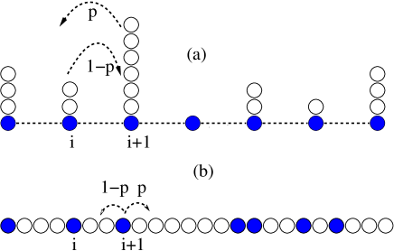
Figure 1: Mapping between (a) the short range ZRP and (b) the traffic model. (a) Sites are shown by filled circles and particles by open circles. Here a particle hops from the $i+1$th site which is more populated to the $i$th site with probability $p$ and from the $i$th site to $i+1$th site with probability $1-p$. (b) The corresponding traffic problem in one dimension, where the occupation number corresponds to the number of empty sites (open circles) to the right of the vehicles (filled circles) and the motion is towards the neighbour located further with probability $p$.

We intend to obtain the particle distribution function $P(n)$ as time $t\to\infty$, i.e., the probability that there are $n$ particles on a site in the steady state for different values of $p$ with a fixed value of $\rho$.

For the limiting case $p=1$, there will be hops to lesser populated sites always. A steady state will correspond to all sites having identical number of particles equal to $\rho$ ($\rho\geq 1$) if there were no transfers between equally populated sites. However, since we allow transfers even in this case, one may expect the probability $P(n)$ to be peaked at $n=\rho$ with a finite width. On the other hand, for small $p$, there will be more transfers from lesser populated sites leading to a tendency of accumulation of particles on a single site which corresponds to a condensate phase. Hence one can expect a transition between the condensate and non condensate phase at a critical value of $p$. The condensate-non-condensate phase transition, if any, is qualitatively similar to the jamming transition in the traffic model; the condensate phase corresponding to the jammed phase. Thus the non-condensate phase is also termed as the fluid phase.

In general, for mass transport models it was found that in the condensate state, $P(n)$ can be analysed using the scaling form satya :

$$P(n)\propto\frac{1}{L^{\gamma+1}}f[\frac{n-M}{L^{\gamma}}],$$ (1)

where $M$ is related to the excess mass. Our goal will be to find out whether a similar scaling form is valid for the present case and the value of the exponent $\gamma$ in the condensate phase. Results are essentially independent of the value of $\rho$ apart from trivial scaling factors and presented for $\rho=5$ for all cases.

III Mean-field approach

The long range model can be regarded as a mean field model for which a master equation for $P(n)$ can be written as

$$\frac{dP(n,t)}{dt} = -p\sum_{m<n}P(n,t)P(m,t)-(1-p)\sum_{m>n}P(n,t)P(m,t)$$ (2)

$$-p\sum_{m>n}P(n,t)P(m,t)-(1-p)\sum_{1\leq m<n}P(n,t)P(m,t)+p\sum_{m<n+1}P(n+1,t)P(m,t)+$$

$$(1-p)\sum_{m>n+1}P(n+1,t)P(m,t)+p\sum_{m>n-1}P(n-1,t)P(m,t)+(1-p)\sum_{1\leq m<n-1}P(n-1,t)P(m,t)$$

$$-2[P(n,t)]^{2}+[P(n+1,t)]^{2}+[P(n-1,t)]^{2}$$

for $n\geq 1$ and

$$\frac{dP(0,t)}{dt} = -p\sum_{m>0}P(0,t)P(m,t)+pP(1,t)P(0,t)+(1-p)\sum_{m>1}P(1,t)P(m,t)+[P(1,t)]^{2}$$ (3)

for $n=0$. Here the transition rates have been assumed to be unity and $t$ taken to be a dimensionless variable. The upper limit in the summations is $\rho L$ unless otherwise restricted. The conditions to be satisfied by $P(n,t)$ are $\sum_{n}P(n,t)=1$ (normalisation) and $\langle n\rangle=\sum_{n}nP(n,t)=\rho$ (conservation) at all times. We have used the notation $P(n,t\to\infty)=P(n)$.

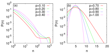
Figure 2: ME: Occupation probability distribution $P(n)$ for (a) lower values of $p$ and (b) higher values of $p$. System size is $L=256$.

Solving these equations numerically, we calculated $P(n)$, the steady state value (see Fig. 2). The initial values $P(n,t=0)$ are taken to be completely random. For lower values of $p$ a bump appears at $n={\mathcal{O}}(\rho L$) indicating the presence of a condensate. A systematic study of the distribution function for small $p$, however, is difficult as the tail of the distribution takes very long time to equilibrate and this leads to accumulation of numerical errors in solving the differential equations. At small $p$, the bump changes shape as the observation time is increased while for small $n$, $P(n)$ remains more or less constant even at later times. Although the evidence of the transition is present in the results as the bump disappears for larger values of $p$, the ME results are less reliable for small $p$ and it is not possible to locate the transition point very accurately. Nevertheless, one can check whether eq. (1) is valid here by plotting the rescaled probabilities for different values of $L$ and achieve a data collapse using trial values of $\gamma$. In Fig. 3, the data for $p=0.05$ are shown where we see that with $\gamma=0.99\pm 0.005$, the data collapse is fairly appreciable.

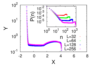
Figure 3: ME: Scaling collapse of occupation probability distribution $P(n)$, where $Y=P(n)L^{\gamma+1}$ has been plotted against $X=\frac{(n-L)}{L^{\gamma}}$. Inset is for the occupation probability distribution $P(n)$ for different system sizes. Particle density is $\rho=5$ and $p=0.05$.

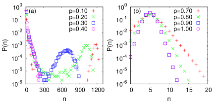
Figure 4: LR: Occupation probability distribution $P(n)$ is for (a) lower values of $p$ and (b) higher values of $p$. System size is $L=256$.

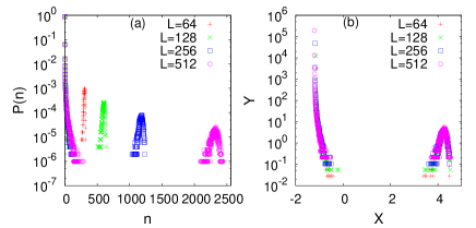
Figure 5: LR: (a) Occupation probability distribution $P(n)$ for different system sizes for $p=0.10$ and (b) the scaling collapse of the same. Here $Y=P(n)L^{\gamma+1}$ has been plotted against $X=\frac{(n-L)}{L^{\gamma}}$. Particle density is $\rho=5$.

IV Results using numerical simulations

In this section we discuss results obtained using numerical simulation considering both the long range and short range models. In general, we have taken systems with size $L\leq 1024$ and taken averages over at least two thousand configurations. Initially, all the sites are randomly occupied. Asynchronous dynamics have been used to update the state of the system.

IV.1 Condensate to fluid phase transition

IV.1.1 Long Range (LR) case

As the master equation (ME) approach poses difficulty to analyse the tail of the distribution for small $p$, we used Monte Carlo simulation to calculate $P(n)$. The steady state results for LR case show clearly the presence of the bump right from $p=0$ up to a value $p=p_{c}$ (see Fig. 4(a)). Simple inspection shows that the transition point $p_{c}$ beyond which the bump vanishes is close to $p=0.33$. It is possible to analyse $P(n)$ for $p<p_{c}$ and do a scaling analysis using data for different values of $L$. We find that indeed the scaling form given by (1) is valid with $M=cL$ as the data for different system sizes collapse to a single curve when an appropriate value of $\gamma$ is used (see Fig. 5). The proportionality constant $c$ is in general equal to $1$ to obtain a good collapse. However, there are some intricacies involved in this choice which is discussed later in section V.

The value of $\gamma$ (Table 1) shows a slow decrease with $p$. This implies the LR case has a non-universal behaviour. This non-universality is presumably related to the fact that the location of the secondary peak in $P(n)$ depends on $p$ as shown in Fig. 4(a).

The estimate of the transition point can be more accurately made from the calculation of fluctuations. In the condensate phase, $P(n)$ has considerably large values only for $n$ close to zero and $\rho L$. As an approximation, one can take $P(n)$ to be a double delta function at these two values, such that

$$P(n)=A\delta(n)+B\frac{1}{L^{\gamma+1}}\delta(\frac{n-cL}{L^{\gamma}}).$$ (4)

The constants $A$ and $B$ can be found out from the conditions $\int P(n)dn=1$ (normalisation condition) and $\int nP(n)dn=\rho$ (fixed average value). This gives

$$A+B/L=1$$

and

$$Bc=\rho.$$

In the thermodynamic limit $B/L$ vanishes giving $A=1$. Using these values, the fluctuation $\sqrt{\langle\Delta n^{2}}\rangle=\sqrt{\langle n^{2}\rangle-{\langle n\rangle}^{2}}$ equals $\sqrt{\rho cL-\rho^{2}}$. Hence to the leading order, $\sqrt{\langle\Delta n^{2}}\rangle$ is $\mathcal{O}(L^{1/2})$ with the proportionality constant equal to $\sqrt{\rho c}$. No $p$ dependence is present here. Also, we note that for small enough $p$, $c$ is very close to $\rho$ as the second bump peaks at $\rho L$ very sharply. Hence in the limit $p\to 0$, $\sqrt{\langle\Delta n^{2}}\rangle$ is given by $\rho L^{1/2}$.

On the other hand, in the fluid phase, the fluctuation should be finite and hence should either remain constant or decrease with $L$. We indeed note from the simulation results that $\sqrt{\langle\Delta n^{2}\rangle}$ increases with $L$ for small $p$ values while for large values of $p$, $\sqrt{\langle\Delta n^{2}\rangle}$ is independent of $L$, shown in Fig. 6(a). We also find that $\sqrt{\langle\Delta n^{2}\rangle}$ shows a general variation as $\sim L^{\alpha}$ for a fixed value of $p$. The value of the exponent is almost constant, $\alpha\sim 0.50$, up to a value of $p$, then it sharply decreases to zero with $p$ (see inset of Fig. 6(a)). One can estimate the transition point $p_{c}$ as the point (approximately) up to which the fluctuation varies as $\sim L^{1/2}$ and we get $p_{c}=0.33\pm 0.02$ from this data. The proportionality constant, theoretically predicted as $\rho=5$ for very small $p$, decreases from about $4.8$ at $p=0$ to close to $4.3$ at $p_{c}$. This variation is not surprising as the value of $c$ depends on $p$. Hence we find very good agreement with the theoretical prediction for the exponent $\alpha$ as well as the associated proportionality constant.

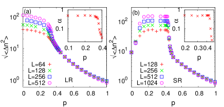
Figure 6: Fluctuation of occupation number $\sqrt{\langle\Delta n^{2}\rangle}$ as a function of $p$ for different system sizes. Inset is for the variation of the exponent $\alpha$ as a function of $p$. (a) long range case (LR) (b) short range case (SR). The error bars are less than the size of the data points.

Table 1: Exponent $\gamma$ for different values of $p$.

$p$	$\gamma$ for $\rho$	$\gamma$ for $\rho$
	$=5$ (LR)	$=5$ (SR)
$0.05$	$0.992\pm 0.002$	-
$0.10$	$0.970\pm 0.003$	-
$0.15$	$0.954\pm 0.003$	$1.000\pm 0.001$
$0.20$	$0.940\pm 0.005$	$1.000\pm 0.001$
$0.25$	$0.910\pm 0.010$	$0.997\pm 0.004$
$0.30$	$0.850\pm 0.01$	$0.997\pm 0.004$
$0.35$	-	$0.995\pm 0.005$
$0.40$	-	$0.998\pm 0.005$

We present snapshots at the steady state in support of the different behaviour of the particle distribution function $P(n)$. We show snapshots for $p=0.05$, $0.45$ and $0.70$. In the first case, there is a condensate forming; even though there are a few sites with finite occupancy, the occupancy of the most populated site is order of magnitude higher than the others (Fig. 7(a)). For $p_{c}<p<0.5$, there are no such unique site indicating the absence of the condensate, however, the fluctuation in the occupancy is appreciable as seen from Fig. 7(b). As $p\to 1$, all sites are occupied with almost equal number ($n\sim\rho$) (Fig. 7(c)).

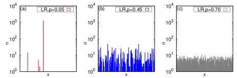
Figure 7: LR: Snapshots of occupation of sites for different values of $p$. System size is $L=256$ and density $\rho=5$. Here $x$ varies from $1$ to $256$.

IV.1.2 Short Range (SR) case

There are some obvious intrinsic differences between the long and the short range processes. For example, in the extreme case of $p=0$, it is expected that many sites will become unoccupied as a rich-gets-richer strategy is imposed. However, the condensate will have difficulty to form in the short range model as the sites which are populated may not interact at all. Hence a large number of sites, separated by finite distances, become populated though none of them have a macroscopically large occupation number. As a result, the distribution function does not show a condensate state. Simulation made for the short range (SR) model shows that this continues up to a value of $p=p_{l}$.

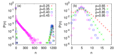
Figure 8: SR: Occupation probability distribution $P(n)$ is for (a) lower values of $p>p_{l}$ and (b) higher values of $p$. System size is $L=256$.

Hence in the short range case, only for $p\gtrsim 0.15$ and $p\lesssim 0.44$, $P(n)$ shows a bump near $\rho L$ and thus there is a non-zero lower bound of $p=p_{l}$ for the condensate to form (see Fig. 8(a) for $P(n)$ at $p>p_{l}$; and section IVB for $P(n)$ at $p<p_{l}$). As in the LR case, the scaling form (1) is also valid here with $M\simeq L$ in SR (see Fig. 9). However, in contrast to the long range case, $\gamma$ is very close to unity and does not show any systematic dependence on $p$ (see Table 1) indicating universal behaviour. This is explained from the fact that the secondary peak positions are almost independent of $p$ except perhaps very close to $p_{l}\simeq 0.15$.

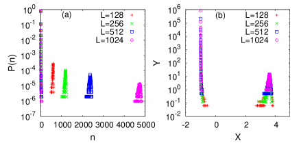
Figure 9: SR: (a) Occupation probability distribution $P(n)$ for different system sizes for $p=0.35$ and (b) the scaling collapse of the same. Here $Y=P(n)L^{\gamma+1}$ has been plotted against $X=\frac{(n-L)}{L^{\gamma}}$. Particle density is $\rho=5$.

Using the same argument as in the LR case, one can estimate $p_{c}$ for the SR case from the data for $\sqrt{\langle\Delta n^{2}\rangle}$. For the SR case also, $\sqrt{\langle\Delta n^{2}\rangle}$ shows system size dependent behaviour for lower values of $p$ only (see Fig. 6(b)). In Fig. 6(b) (inset), we show that here also $\sqrt{\langle\Delta n^{2}\rangle}\sim L^{\alpha}$ with $\alpha$ very close to $0.50$ up to a value of $p$ and shows an even sharper drop beyond this value. The estimated transition point is $p_{c}=0.44\pm 0.01$. The proportionality constant here is not sensitive to the value of $p$ and varies in the range $4.4\pm 0.2$ (theoretical prediction is $5$). This is because the secondary peaks in the condensate phase occur more or less at the same position independent of $p$ in the SR case. Hence once again good agreement is obtained with the theoretical estimates.

We also present snapshots in support of the appearance of the variety of phases. At low values of $p$, ($p<p_{l}$), occupied sites cannot interact as they are separated by empty sites. The snapshot shows occupancy at many sites, mostly separated by one or a few empty sites (Fig. 10(a)). Hence $P(n)$ does not show condensation for $p<p_{l}$ but may show a long tail (details in section IVB). In the condensed phase $p_{c}>p>p_{l}$, a finite fraction of particles lies in a single site (Fig. 10(b)). Immediately above $p_{c}$, the melting of the condensate state is manifested as we see the majority of particles populating a cluster of sites slowly disappear in the bulk as $p$ is increased (Figs. 10(c)-10(e)). For even higher value of $p$, all sites are almost equally occupied ($n\sim\rho$) as in LR.

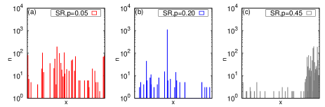
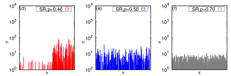
Figure 10: SR: Snapshots of occupation of sites for different values of $p$. System size is $L=256$ and density $\rho=5$. Here $x$ varies from $1$ to $256$.

IV.1.3 Signature of the phase transition point in other quantities

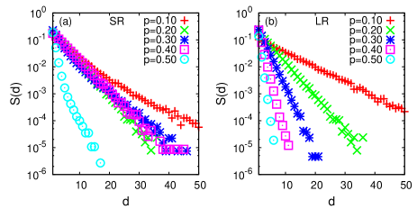
Figure 11: Distribution of interval size $S(d)$ for different values of $p$. Left panel is for the short range model and right one is for the long range model. System size is $L=256$ and density $\rho=5$.

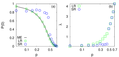
Figure 12: (a) Fraction of empty sites $P(0)$ as a function of $p$ for ME, LR and SR methods. (b) Variation of decay exponent of separation of two occupied sites $\lambda$ with $p$ for LR and SR methods.

The signature of the transition point is present in the variation of several quantities in the short range case. The distribution $S(d)$ for the interval size $d$ between two occupied sites is calculated which shows an exponential decay: $S(d)\propto\exp(-\lambda d)$ for all $p$ (Fig. 11). The decay becomes sharper as $p$ increases. $S(d)$ has been fitted with the form $\sim\exp(-\lambda x)$ and $\lambda$ has been estimated for all values of $p$. The exponent $\lambda$ increases continuously with $p$ for LR but for SR $\lambda$ is found to remain rather small up to $p_{c}$ and it increases rapidly beyond this point in the SR model (see Fig. 12(b)). This corresponds to having large intervals below $p_{c}$. Few occupied sites are found for $p_{l}<p<p_{c}$ and the variation of $\lambda$ with $p$ is a quantitative verification of that.

In the condensate phase, number of empty sites is appreciably large while as $p\rightarrow 1$, all sites become occupied. Fraction of empty sites $P(0)$ in the steady state has been studied for both the long and short range cases (see Fig. 12(a)). An estimate is also available from the ME approach which gives steady state values for all $p$ for small $n$. No special behaviour is noted in $P(0)$ at $p_{c}$ in the long range model. On the other hand, the short range case clearly shows a jump in $P(0)$ at $p_{c}$. Once again the long range model, expectedly, does not show any special behaviour.

IV.2 Nature of $P(n)$ in different phases: a comparative picture

In this subsection we present a detailed study of the functional behaviour of the distribution $P(n)$ in different phases. The behaviour of $P(n)$ in the condensate phase ($p_{l}<p<p_{c}$) has already been discussed. Exactly at $p_{c}$, the behaviour is expected to be a power law. Since numerical estimate of $p_{c}$ cannot be exact, one can only verify this for $p$ close to $p_{c}$ and a reasonably good agreement is indeed found. The entire region $p>p_{c}$ is a fluid phase. In the short range case, one may also interpret the $p<p_{l}$ region as a fluid phase as the condensate is absent. However, at $p=0$ the system enters an absorbing (or frozen) state and even for $<0<p<p_{l}$, the dynamics are quite restricted. We thus identify this region as a pseudo frozen phase. We note the tendency of developing a bump at larger values of $n$ as $p\to p_{l}\simeq 0.15$ (Fig. 13).

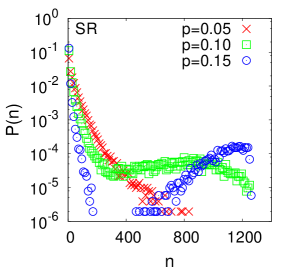
Figure 13: SR: Distribution of occupation number $P(n)$ for $p\leqslant p_{l}$ for SR. System size is $L=256$ and density $\rho=5$.

For $0.5>p>p_{c}$, there is a considerable number of sites which are near empty. In the SR case, an interesting feature is noted: the occupied sites form a cluster which vanishes gradually as $p\to 0.5$ (see snapshots in Figs. 10). This is a kind of “melting” of the highly occupied site which exists up to $p=p_{c}$. The LR case shows no such features for $p>p_{c}$; naturally in the globally connected case, such local correlations cannot exist.

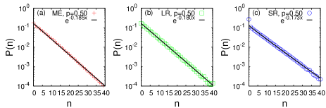
Figure 14: Distribution of occupation number $P(n)$ for $p=0.5$ for (a) ME, (b) LR and (c) SR. System size is $L=256$ and density $\rho=5$.

Both in the long and short range cases, for $p>0.5$, $P(n)$ shows the presence of a peak (i.e. a most probable value) indicating the emergence of a scale. In fact for $p>0.5$, the two models give almost identical results and the results from ME being more reliable as $p$ increases, also show very good agreement. Between $p=0.5$ and 1, $P(n)$ interpolates between a perfectly exponential and a Gaussian form.

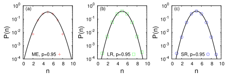
Figure 15: Distribution of occupation number $P(n)$ and fitted curve using equation 5 for $p=0.95$ for (a) ME, (b) LR and (c) SR. System size is $L=256$ and density $\rho=5$.

$P(n)$ decreases exponentially with $n$ at $p=0.5$ for all the three cases (Fig. 14). The fitting form is $A\exp(-bx)$. The exponents are (1) ME: $A=0.169$, $b=0.185$; (2) LR: $A=0.166$, $b=0.181$; (3) SR: $A=0.119$, $b=0.154$. Hence although the qualitative behaviour is independent of the range, the value of the exponent $b$ is case sensitive. We also note the very good agreement of the results obtained from ME and LR.

For large values of $p$ ($p>0.5$), $P(n)$ can be fitted to a Gaussian form for ME, LR and SR methods (Fig. 15). Fittings show better agreement as $p\rightarrow 1$ and width of the distribution decreases with $p$. The Gaussian form is:

$$f(x)\sim e^{-a(n-\tilde{n})^{2}}.$$ (5)

The value of $a$ and $\tilde{n}$ are listed in Table II.

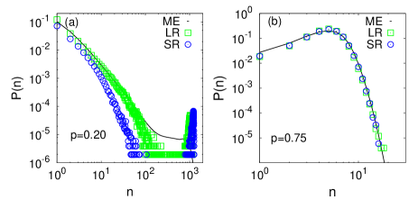
Figure 16: (a) Distribution of occupation number $P(n)$ for $p=0.20$. (b) Distribution of occupation number $P(n)$ for $p=0.75$. System size is $L=256$ and density $\rho=5$.

Table 2: Table for the estimates of the values of the exponents $a$ and $\tilde{n}$ using equation (5).

$p$	$a$ for	$\tilde{n}$ for	$a$ for	$\tilde{n}$ for	$a$ for	$\tilde{n}$ for
	ME	ME	LR	LR	SR	SR
$0.55$	$0.014$	$0.892$	$0.019$	$1.910$	$0.013$	$0.664$
$0.60$	$0.034$	$3.984$	$0.043$	$4.215$	$0.023$	$3.523$
$0.65$	$0.060$	$4.682$	$0.077$	$4.761$	$0.058$	$4.777$
$0.70$	$0.092$	$4.895$	$0.121$	$4.926$	$0.105$	$4.972$
$0.75$	$0.128$	$4.967$	$0.177$	$4.982$	$0.163$	$5.010$
$0.80$	$0.169$	$4.990$	$0.244$	$4.991$	$0.231$	$5.007$
$0.85$	$0.214$	$4.997$	$0.316$	$5.000$	$0.307$	$5.007$
$0.90$	$0.259$	$4.999$	$0.391$	$5.000$	$0.390$	$5.007$
$0.95$	$0.306$	$4.999$	$0.468$	$5.000$	$0.480$	$5.007$
$1.00$	$0.352$	$4.999$	$0.541$	$5.000$	$0.546$	$5.000$

In the condensed phase, $P(n)$ is quite different for the LR and SR cases. As mentioned before, the secondary peak of the distribution occurs very close to $n=\rho L$ for SR model while for LR model, the peak position changes to lesser values of $n$ as $p$ approaches $p_{c}$. Fig. 16(a) shows that the actual values of $P(n)$ for LR and SR differ appreciably even for small $n$ for a fixed value of $p$ in the condensate phase. The results from the ME approach, as mentioned before, does not show perfect agreement with the LR results at larger values of $n$ due to computational difficulties at low $p$ values. But in the fluid phase, there is very good agreement of the values of $P(n)$ for all the three methods (Fig. 16(b)).

V Summary and discussions

In summary, we have studied a general form of the the well known zero range process. A condensate phase is obtained keeping the density constant and tuning the hopping probability $p$. A variety of rich behaviour is observed as $p$ is increased; the system passes through different phases for $0\leq p<p_{l}$, $p_{l}<p\leq p_{c}$, $p_{c}<p<0.5$ and beyond $p=0.5$. Severals snapshots are presented which show the system configuration in the different phases.

Naively one would expect $p_{c}$, the point below which a condensate phase forms, to be equal to $0.5$ as hopping from lesser populated sites are more probable below $p=0.5$. However we get $p_{c}<0.5$ for both the SR and LR models. This is due to the reason that when an empty site is involved, the other site will always get less populated, which makes the probability of forming the condensate lesser. Why the short range process has a higher $p_{c}$ compared to the long range case may be explained from the fact that when an occupied site becomes isolated in the former, no more transfer takes place from it.

Our results are mainly based on finite size scaling analysis. The choice of parameters for the data collapse of $P(n)$ is a tricky question and we have taken the values which give the manifestly best collapses. In particular, if the value of the exponent $\gamma$ is close to unity the data collapses for the secondary bump in $P(n)$ are not sensitive to the value of $c$ for obvious reasons. However, for the long range case, $\gamma$ deviates from unity at larger values of $p$ and the best collapses are obtained for $c=1$ in general. Hence, we have used $c=1$ everywhere in the plots of the data collapse.

The transition points as well as the exponent associated with the scaling function for the particle number distribution function depend on the range of interaction. Only the short range case shows universality. Excellent agreement is reached for the analytical and simulation methods (for LR) when reliable steady state values can be obtained while solving the master equation numerically. The model shows range independent behaviour for $p>0.5$ where a typical scale emerges. $P(n)$ is exponential for $p=p_{c}$ while it can be approximated by a Gaussian form deep inside the fluid phase.

Acknowledgements: AK acknowledges financial support from UGC sanction no. F.7-48/2007(BSR). PS acknowledges financial support from CSIR (Govt. of India) project. The authors thank Satya N. Majumdar for very helpful discussions and suggestions.

References

- (1) O. J. O’Loan, M. R. Evans and M. E. Cates, Phys. Rev. E 58, 1404 (1998).
- (2) D. Chowdhury, L. Santen and A. Schadschneider, Phys. Rep. 329, 199 (2000).
- (3) J. Kaupuˇzs, R. Mahnke, and R. J. Harris, Phys. Rev. E 72, 056125 (2005).
- (4) P. Bialas, Z. Burda and D. Johnston, Nucl. Phys. B493, 505 (1997).
- (5) P. L. Krapivsky, S. Redner and F. Leyvraz, Phys. Rev. Lett. 85, 4629 (2000).
- (6) G. Bianconi and A. L. Barabási, Phys. Rev. Lett. 86, 5632 (2001).
- (7) J. P. Bouchaud and M. M ̵́ezard, Physica A 282, 536 (2000).
- (8) Z. Burda, D. Johnston, J. Jurkiewicz, M. Kaminski, M. A. Nowak, G. Papp and I. Zahed, Phys. Rev. E 65, 026102 (2002).
- (9) K. van der Weele, D. van der Meer, M. Versluis and D. Lohse, Europhys. Lett. 53, 328 (2001).
- (10) Satya N. Majumdar, M. R. Evans and R. K. P. Zia, Phys. Rev. Lett. 94 180601 (2005).
- (11) M. R. Evans, S. N. Majumdar and R. K. P. Zia, J. Stat. Phys. 123 357 (2006).
- (12) B. Waclaw, J. Sopik, W. Janke and H. Meyer-Ortmanns, Journal of Statistical Mechanics: Theory and Experiment P10021 (2009).
- (13) F. Spitzer, Adv. Math. 5 246 (1970).
- (14) M. R. Evans and T. Hanney, J. Phys. A 38 R195 (2005).
- (15) Y. Kafri, E. Levine, D. Mukamel, G. M. Schutz and J. Török, Phys. Rev. Lett. 89 035702 (2002).
- (16) M. R. Evans, E. Levine, P. K. Mohanty and D. Mukamel, Eur. Phys. J. B 41 223 (2004).
- (17) S. Großkinsky, G. M. Schütz and H. Spohn, J. Stat. Phys. 113 389 (2003).
- (18) C. Godrèche and J. -M. Luck, J. Phys. A 38 7215 (2005).
- (19) I. Jeon, P. March and B. Pittel, Ann. Probab. 28 1162 (2000).
- (20) P. A. Ferrari, C. Landim and V. V. Sisko., J. Stat. Phys. 128 1153 (2007).
- (21) I. Armendáriz and M. Loulakis, Prob. Theory Related Fields 145 175 (2009).
- (22) I. Armendáriz and M. Loulakis, Stoch. Proc. Appl. 121 1138 (2011).
- (23) B. Waclaw, J Sopik, W. Janke and H. Meyer-Ortmanns, J. Phys. A 42 315003 (2009).
- (24) M. R. Evans, T. Hanney, and S. N. Majumdar, Phys. Rev. Lett. 97 010602 (2006).
- (25) J. M. Luck and C. Godrèche J. Stat. Mech. (2007) P08005.
- (26) M. R. Evans and B. Wacklaw, J. Phys. A 47 095001 (2014).
- (27) C. Cocozza-Thivent, Z. Wahrscheinlichkeits, theor. Verwandte Geb. 70 509 (1985).
- (28) S. Biswas, P. Sen and P. Ray, J. Phys.: Conf. Ser. 297 012003 (2011).