Formation and plasma circulation of solar prominences

Abstract

Solar prominences are long-lived cool and dense plasma curtains in the hot and rarefied outer solar atmosphere or corona. The physical mechanism responsible for their formation and especially for their internal plasma circulation has been uncertain for decades. The observed ubiquitous down flows in quiescent prominences are difficult to interpret as plasma with high conductivity seems to move across horizontal magnetic field lines. Here we present three-dimensional numerical simulations of prominence formation and evolution in an elongated magnetic flux rope as a result of in-situ plasma condensations fueled by continuous plasma evaporation from the solar chromosphere. The prominence is born and maintained in a fragmented, highly dynamic state with continuous reappearance of multiple blobs and thread structures that move mainly downward dragging along mass-loaded field lines. The prominence plasma circulation is characterized by the dynamic balance between the drainage of prominence plasma back to the chromosphere and the formation of prominence plasma via continuous condensation. Plasma evaporates from the chromosphere, condenses into the prominence in the corona, and drains back to the chromosphere, establishing a stable chromosphere-corona plasma cycle. Synthetic images of the modeled prominence with the Solar Dynamics Observatory Atmospheric Imaging Assembly closely resemble actual observations, with many dynamical threads underlying an elliptical coronal cavity.

1 INTRODUCTION

Solar prominences are about 100 times denser and cooler than their surrounding hot corona, with their weight supported by the magnetic field against gravity. They exist for days to weeks above polarity inversion lines (PIL), which separate positive and negative magnetic flux regions in the photosphere. Prominences are frequently found inside coronal cavities, which are tunnel-like elliptical dark regions (Gibson et al., 2010) at the solar limb, with up to 40 % density depletion (Fuller et al., 2008), around the prominences. The magnetic structure hosting a prominence and its cavity is believed to be a helical magnetic flux rope confined by overlying magnetic loops, which is consistent with observed spinning plasma motions (Wang & Stenborg, 2010) as well as linear polarization signatures (Bak-Stȩślicka et al., 2013). A flux rope was present in early two-dimensional (2D) theoretical prominence models (Kuperus & Raadu, 1974) and 2D magnetohydrostatic solutions for prominence-embedded flux ropes have been demonstrated analytically (Low & Zhang, 2004) and numerically (Blokland & Keppens, 2011; Hillier & van Ballegooijen, 2013).

Static prominence models assume that quiescent prominences change little with time. However, high resolution observations have found that quiescent prominences consist of fine and vertically oriented plasma threads, that continuously evolve with downward motions (4 to 35 km s^-1) (Engvold, 1976; Berger et al., 2008; Chae et al., 2008). Moreover, episodic dark plumes may rise (Berger et al., 2008, 2011) from the bottom of prominences and propagate upward between threads with speeds about 10 to 20 km s^-1. The heavy prominence material suspended above the light coronal plasma can be liable to Rayleigh–Taylor (RT) instability (Ryutova et al., 2010) which has been investigated in several numerical magnetohydrodynamic (MHD) models (Khomenko et al., 2014; Hillier et al., 2011; Terradas et al., 2015; Keppens et al., 2015). However, none of these models addressed prominence formation and mass cycling, or studied a realistic 3D flux rope.

The idea that prominences form via in situ condensation of coronal plasma was inferred from thermal instability theory (Parker, 1953; Field, 1965) and is supported by observations in extreme ultraviolet (EUV) channels (Liu et al., 2012; Berger et al., 2012). Moreover, continuous condensations must happen to compensate mass loss of quiescent prominences, which requires an incessant supply of hot plasma from chromosphere to corona. Such hot plasma flows have not been convincingly detected, although persistent horizontal flows of H$\alpha$-emitting cool plasma originating from the chromosphere into a prominence was observed (Chae et al., 2008) and the episodic dark rising plumes filled with hot plasma may provide a small fraction of the needed mass (Berger et al., 2010). Numerical modeling of condensations as a result of runaway radiative cooling started with one-dimensional hydrodynamic simulations along individual magnetic field lines (Antiochos et al., 1999; Karpen et al., 2001; Xia et al., 2011; Luna et al., 2012) and progressed in recent years to 2D MHD simulations in magnetic arcades (Xia et al., 2012; Keppens & Xia, 2014). These models add localized heating at footpoints of magnetic loops to evaporate plasma from chromosphere to corona leading to continuous condensations. However, restricted by 1D or 2D setups, they cannot fully establish the internal dynamics of prominences. Recent work on prominence formation via in situ condensation in a 2D (Kaneko & Yokoyama, 2015) and 3D flux rope (Xia et al., 2014a) did not reproduce internal dynamics and mass drainage and only found a small prominence fragment that settled in a magnetostatic equilibrium.

We here report a set of 3D models that for the first time ever demonstrate continuous formation of prominence condensations in a coronal cavity, achieving a balanced chromosphere-corona plasma cycle characterized by vertical flows in thin prominence threads. The numerical methods and the simulation procedure are explained in Section 2. We present the results in Section 3. Finally, the results are discussed in Section 4.

2 SIMULATION STRATEGY

Since the magnetic topology of quiescent prominences is believed to be an elongated magnetic flux rope, we first perform isothermal MHD simulations to simulate the formation of a magnetic flux rope driven by footpoint motions and flux cancellation (van Ballegooijen & Martens, 1989; Xia et al., 2014b). Our 3D model is set up in a Cartesian box covering 200 Mm $\times$ 120 Mm $\times$ 80 Mm , in $x$ (-100 Mm to 100 Mm), $y$ (-60 Mm to 60 Mm), and $z$ (0 to 80 Mm) directions, where a finite beta corona of 1 MK constant temperature is initially constructed with density and gas pressure prescribed from hydrostatic equilibrium with a bottom $10^{9}$ cm^-3 number density. We start from a bipolar magnetic field in the shape of an elongated sheared arcade. This arcade field itself is generated by linear force-free field extrapolation from an analytically prescribed bipolar magnetogram with two opposite polarity regions shaped like two parallel baguettes. This magnetogram $B_{m}$ is formulated as:

$$B_{m}=\begin{cases}B_{0}\exp(-\frac{(x-x_{1}+x_{L})^{2}}{2\delta x^{2}}-\frac{(y-y_{1})^{2}}{2\delta y^{2}})-B_{0}\exp(-\frac{(x-x_{2}+x_{L})^{2}}{2\delta x^{2}}-\frac{(y-y_{2})^{2}}{2\delta y^{2}})&\text{if $x<x_{1}-x_{L}$}\\ B_{0}\exp(-\frac{(y-y_{1})^{2}}{2\delta y^{2}})-B_{0}\exp(-\frac{(y-y_{2})^{2}}{2\delta y^{2}})&\text{if $x_{1}-x_{L}\leq x\leq x_{1}+x_{L}$}\\ B_{0}\exp(-\frac{(x-x_{1}-x_{L})^{2}}{2\delta x^{2}}-\frac{(y-y_{1})^{2}}{2\delta y^{2}})-B_{0}\exp(-\frac{(x-x_{2}-x_{L})^{2}}{2\delta x^{2}}-\frac{(y-y_{2})^{2}}{2\delta y^{2}})&\text{if $x>x_{1}+x_{L}$}\\ \end{cases}$$

where $B_{0}=20$ G, $x_{1}=x_{2}=0$ Mm, $y_{1}=-y_{2}=25$ Mm, $x_{L}=50$ Mm, $\delta x=10$ Mm, and $\delta y=13$ Mm. An exact Green’s function method (Chiu & Hilton, 1977) is used to generate an initial linear force-free field with constant $\alpha=-0.08$. Since our simulation box is intended to start at low chromospheric heights, this magnetogram is placed 4 Mm below the bottom plane of the simulation box.

A composite surface flow is imposed at the bottom boundary with the formula as:

$$v_{y}^{b}=-f(t)C_{1}\frac{\partial|B_{m}|}{\partial y}\exp(-y^{2}/y_{d}^{2}),v_{x}^{b}=-v_{y}^{b}$$

where $y_{d}=35$ Mm quantifies an additional Gaussian width parameter away from the polarity inversion line (PIL), $f(t)$ is a linear ramp function to switch on and off the driving flow, and the amplitude factor $C_{1}$ is chosen so that the driving speed has a maximum value of 12.8 km s^-1 and the maximum initial Alfvén Mach number is 0.0155. The flow is a combination of a shearing flow and a converging flow relative to the PIL. The shearing flow roughly mimics the effective shearing of an east-west bipolar arcade by the differential rotation of the solar surface. The converging flow from the strong field regions to weak field regions is an effective result of magnetic element diffusion caused by random supergranular motions (Leighton, 1964). Flows far away from the PIL are suppressed by the exponential factor for an easier handling of the side boundaries.

The model evolution is performed by solving the isothermal MHD equations given by

$$\frac{\partial\rho}{\partial t}+\nabla\cdot\left(\rho\mathbf{v}\right) =0,$$ (1)

$$\frac{\partial\left(\rho\mathbf{v}\right)}{\partial t}+\nabla\cdot\left(\rho\mathbf{vv}+p_{\rm tot}\mathbf{I}-\frac{\mathbf{BB}}{\mu_{0}}\right) =\rho\mathbf{g},$$ (2)

$$\frac{\partial\mathbf{B}}{\partial t}+\nabla\cdot\left(\mathbf{vB}-\mathbf{Bv}\right) =0,$$ (3)

where $\rho$, $\mathbf{v}$, $\mathbf{B}$, and $\mathbf{I}$ are the plasma density, velocity, magnetic field, and unit tensor, respectively, while the total pressure is $p_{\rm tot}\equiv p+\frac{B^{2}}{2\mu_{0}}$ and $\mathbf{g}=-g_{\odot}r_{\odot}^{2}/(r_{\odot}+z)^{2}\mathbf{\hat{z}}$ is the gravitational acceleration with $r_{\odot}$ the solar radius and $g_{\odot}$ the solar surface gravitational acceleration. To normalize the equations for computation, we use 10 Mm, $10^{9}$ cm^-3, 116.45 km s^-1 , and 2 Gauss as the unit of length, number density, velocity, and magnetic field, respectively. We use the Adaptive Mesh Refinement (AMR) Versatile Advection Code (MPI-AMRVAC) (Keppens et al., 2012; Porth et al., 2014) to numerically solve these equations with a third-order accurate scheme combining a Harten-Lax-van Leer scheme (Harten et al., 1983) with a third-order limited reconstruction (Čada & Torrilhon, 2009) and a three-step Runge–Kutta time integration. To numerically maintain close to zero divergence of the magnetic field, we use the Generalized Lagrangian Multiplier method (Dedner et al., 2002). The model domain at this phase is discretized on a three-level AMR grid which has an effective resolution of $400\times 240\times 240$ with the smallest cells of 500 km $\times$ 500 km $\times$ 333 km. The simulation setup is completed by the following boundary conditions. We force zero vertical velocity on the bottom face and zero velocity on the other five faces of the box by antisymmetric boundary conditions. We extrapolate the magnetic field at the bottom boundary and the top boundary from inner physical values, keeping the normal gradient zero, with a one-sided third-order finite difference representation. Then we modify the normal component to enforce the divergence-free condition in a second-order centered difference evaluation. The magnetic fields at the four side boundaries are kept fixed. The density values in the side boundary cells are copied from the neighbouring cells of the physical domain. We fix the gravitationally stratified density at the bottom and adopt a gravitationally stratified density profile at the top.

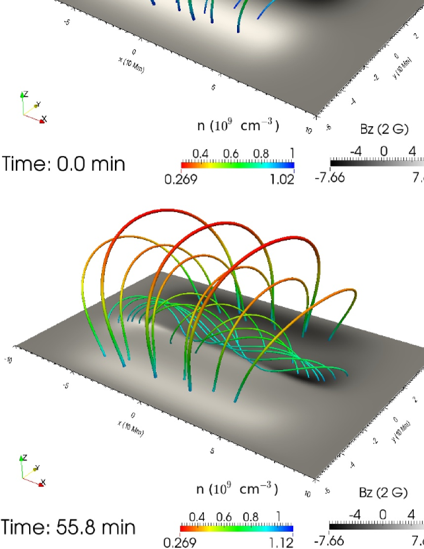
Figure 1: The formation process of a magnetic flux rope in the solar corona. In these panels depicting six subsequent moments, magnetic field lines colored by number density ($n$) show the forming flux rope and overlying arcade loops and greyscale of the bottom plane indicating vertical magnetic field strength.

The bottom flows drive those coronal loops that root in the inner halves of the main arcade polarities to move towards aligning with the PIL. As footpoints from opposite polarities collide on the PIL, magnetic reconnections occur due to finite numerical resistivity, to join arched loops into helical loops in a head-to-tail style. These helical loops, winding about the same central axial field line, form a helical magnetic flux rope (see Figure 1). We completely switch off the driving flows after 100 minutes and let the flux rope relax to an equilibrium state. In the end of this stage, a large-scale elongated flux rope is formed with its flux surface touching the bottom plane. The length of the flux rope is about 160 Mm and the diameter of its cross section is about 34 Mm. The density distribution does not change much compared to the initial state and the magnetic field has negligible Lorentz force.The magnetic field strength of the flux rope is about 6 to 7 Gauss which is consistent with the field strength of a quiescent prominence since spectral polarimetric measurements show that the magnetic field in a quiescent prominence ranges from 3 to 30 G and it is predominantly horizontal making an acute angle with respect to the axis of the prominence (Leroy et al., 1983; Bommier et al., 1994; Orozco Suárez et al., 2014).

In the second stage, we perform a full MHD simulation to produce a modeled solar atmosphere in thermal equilibrium containing the magnetic flux rope which was generated in the isothermal MHD modeling described above. To setup the initial state based on the isothermal flux rope, we kept the magnetic field unchanged and modified the density and temperature profiles from their isothermal states to a static vertically stratified solar atmosphere including chromosphere, transition region, and corona. We set the region below a height of 2.7 Mm to have chromospheric temperature 9600 K and above this height, the temperature increases with height in such a way that the vertical thermal conduction flux has a constant value of $2\times 10^{5}$ erg cm^-2 s^-1. The density is then derived assuming a hydrostatic atmosphere with the number density at the bottom being $1.1\times 10^{13}$ cm^-3. We now consider the full MHD equations with the energy equation as:

$$\frac{\partial E}{\partial t}+\nabla\cdot\left(E\mathbf{v}+p_{\rm tot}\mathbf{v}-\frac{\mathbf{BB}}{\mu_{0}}\cdot\mathbf{v}\right)=\rho\mathbf{g}\cdot\mathbf{v}+H-R+\nabla\cdot\left(\boldsymbol{\kappa}\cdot\nabla T\right),\\$$ (4)

where total pressure $p_{\rm tot}\equiv p+B^{2}/2\mu_{0}$, gas pressure $p=2.3n_{\rm H}k_{\rm B}T$, and total energy $E=p/(\gamma-1)+\rho v^{2}/2+B^{2}/2\mu_{0}$. We again use MPI-AMRVAC with the same combination of schemes as the isothermal model. The field-aligned ($\boldsymbol{\kappa}=\kappa_{\parallel}\mathbf{\hat{b}\hat{b}}$) thermal conduction is solved separately using a Runge-Kutta type Super Time Stepping scheme (Meyer et al., 2012) and $\kappa_{\parallel}=10^{-6}T^{5/2}$ erg cm^-1 s^-1 K^-1 is the Spitzer conductivity. Optically thin radiative cooling $R=1.2n_{\rm H}^{2}\Lambda(T)$ is added using an exact integration scheme (Townsend, 2009). To maintain a hot corona, the coronal heating is simulated by adding the parametrized heating term $H=H_{0}=c_{0}e^{-z/\lambda}$ with $c_{0}=10^{-4}$ erg cm^-3 s^-1 and $\lambda=60$ Mm. We increased the highest AMR level of the mesh to 4, resulting in an effective resolution of $800\times 480\times 480$ with the smallest cells of 250 km $\times$ 250 km $\times$ 166 km. We modified the boundary conditions from the isothermal model to set zero velocity and fixed magnetic field at all boundaries. The gas pressure is fixed at the bottom and flexible at the top according to gravitational stratification. At side boundaries, the gas pressure copies values from the inner layer in the physical domain. This modified plasma state is not in thermal equilibrium, so we numerically solve the full MHD equations involving optically thin radiative loss, anisotropic thermal conduction and coronal heating until the system relaxes to a quasi-equilibrium after 114.5 minutes. Our endstate in this phase is reached when all thermal quantities settle into a stable 3D configuration where the magnitude of the remaining velocity is less than 10 km s^-1 and it is representative of a stable flux rope configuration with hot coronal plasma trapped inside it, where twisted field lines connect chromospheric to coronal plasma regions.

In the third stage, we aim to form the macroscopic prominence in the stable flux rope obtained in the second stage. In order to simulate the chromospheric evaporation, which is an efficient way to bring material from the chromosphere to the corona, a relatively strong localized heating $H_{1}$ is added to the energy equation in addition to the global coronal heating $H_{0}$, namely, $H=H_{0}+H_{1}$. We only add the localized heating $H_{1}$ in two fixed cylinders which coincide with the two footpoint regions of the flux rope. These two cylinders are centered on $(x,y)$ positions on the bottom plane at (64, 6) Mm and (-64, -6) Mm, with a radius of 20 Mm. Within them, $H_{1}$ is constant in the chromosphere and decays rapidly with height above the approximate location of the transition region:

$$H_{1}=\begin{cases}f(t)c_{1}e^{-((z-zh)/H_{m})^{2}}&\text{if $z>zh$}\\ f(t)c_{1}&\text{if $z\leq zh$}\end{cases}$$

where $c_{1}=10^{-2}$ erg cm^-3 s^-1, $zh=5$ Mm and $H_{m}=3.16$ Mm. This final stage is simulated for a total of over four hours, and it is this stage which is presented in what follows.

3 RESULTS

As chromospheric plasma gets evaporated into the corona, the lower part of the flux rope slowly evolves into a thermally unstable situation due to the dominating radiative cooling. After about 100 minutes of gradual evolution, we then witness the runaway cooling stage when the decrease of temperature amplifies the radiation, leading to the formation of dynamic blobs and threads. To get an overall impression of the evolution, we quantify the temporal evolution of the mass, the average density, as well as the average velocity of all prominence plasma and all coronal plasma in the computational box (see Figure 2a,b). In this quantification, prominence plasma has its number density higher than $10^{10}$ cm^-3, its temperature lower than 20,000 K, and its altitude higher than 8 Mm. The change in local density and temperature conditions ultimately reaches the threshold to trigger thermal instability, with plasma condensations forming at a rapid pace after 80 minutes, accompanied by a decrease in coronal mass. At time 134.5 minutes, the mass of the prominence reaches a maximal $3.1\times 10^{13}$ g, to then start decreasing as some blobs have by now fallen into the chromosphere. After 164.5 minutes, the mass of the prominence settles and starts to oscillate around an average value of $1.65\times 10^{13}$ g while the mass of the coronal volume reaches a stable value of $8.3\times 10^{14}$ g. The number density of the prominence instantly adopts a value consistent with observations, as it oscillates around a mean value of $1.88\times 10^{10}$ cm^-3. The average temperature of the prominence and the corona are 17,500 K and 1,660,000 K, respectively. For the entire 80 minutes following, we see lots of dynamics in the prominence as a whole, but the drainage of prominence mass into the chromosphere is balanced by new-born prominence material in continuously forming condensations.

If we concentrate on the later stable phase after 164.5 minutes, the average vertical velocity of the prominence plasma is $-4.87$ km s^-1, showing that the prominence plasma is generally descending at a speed much slower than free-fall speed, which is consistent with observations (Liu et al., 2012). To understand the mass flows, we quantify the mass flux through a horizontal plane at the bottom of the corona, including the total mass flux as well as contributions from prominence plasma, coronal plasma, and prominence-corona transition region (PCTR) plasma (Figure 2c). Because of the chromospheric evaporation, the upward mass flux increases in the first 7 minutes and then decreases, impeded by the build-up of a high gas pressure inside the flux rope. As soon as the condensations begin, the evaporating mass flow increases slowly and then gradually settles at around $3.1\times 10^{12}$ g s^-1. Prominence plasma with surrounding PCTR plasma starts to fall down through this plane back into the chromosphere after 110 minutes. The corresponding mass fluxes of prominence plasma and PCTR plasma oscillate with time and eventually stabilize at around $-10^{12}$ g s^-1 and $-2.1\times 10^{12}$ g s^-1, respectively. The total mass flux oscillates around zero, implying a dynamical equilibrium where a steady mass cycling is fully operational. We can draw the analogy with the water cycle on Earth, since we have solar chromospheric plasma that evaporates from the footpoints of the flux rope to reach higher altitudes into the corona where radiative condensations accumulate mass in prominence blobs that ultimately fall back to the chromosphere.

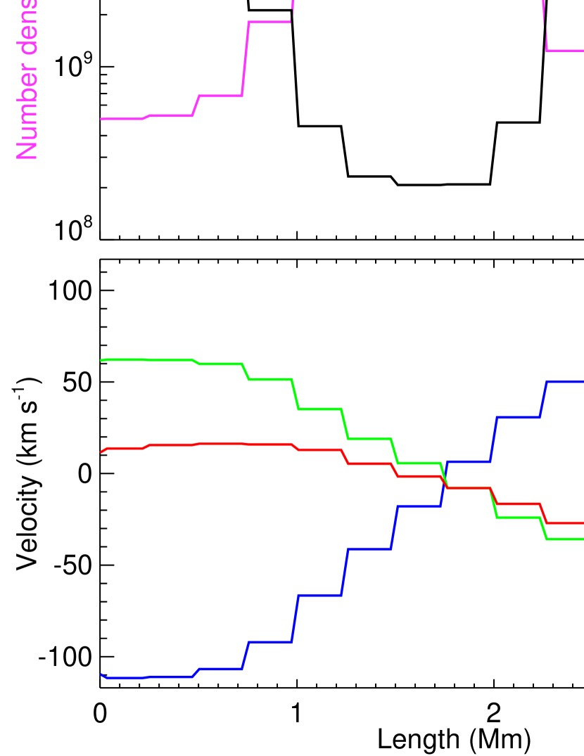
Figure 3: Prominence, magnetic field lines and shearing flows at time 203.2 minutes. a, a global view of the prominence with the yellow translucent density contours at $4\times 10^{9}$ cm^-3, the red density contours at $10^{10}$ cm^-3, magnetic field lines (colored by temperature Te) threading through the prominence, a purple magnetic field line representing the axis of the flux rope, and the bottom plane colored by $B_{z}$. b, close-up view of the region in white rectangular box in a with a white straight line cutting through a thread and the number density (pink curve), temperature (black curve) and velocities (blue curve $V_{x}$, green curve $V_{y}$, red curve $V_{z}$) along the cutting line displayed in c.

The most striking finding of our model is the extremely dynamic and intrinsically fragmented appearance of the prominence matter, from its first instant of formation throughout its steady plasma cycle. The prominence plasma is born in thin threads and blobs distributed over different places in the flux rope as visualized for a particular instant in Figure 3a. Some of the blobs appear and then reside in the central dipped region of fairly left-right symmetrical, twisted field lines. Some blobs form and then surf along the shallow elbows of asymmetrically twisted field lines. A few blobs also pop up and then seemingly follow arched regions of weakly twisted field lines. Although every condensation has a different size and shape, the cross sections perpendicular to their long axis are roughly round. The diameter of these cross sections range from 1000 km to 1800 km. A typical variation of the temperature, density and velocity field across an individual blob is shown for the thread in the zoomed panel of Figure 3b. There are typically shearing flows at both sides of the thread (Figure 3c). These flows themselves influence the thread dynamical evolution and the velocity difference across the thread reaches up to 115 km s^-1 with local Alfvén Mach number up to 1.

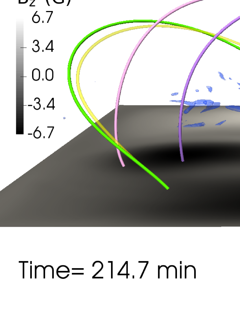
Figure 4: Falling prominence blobs dragging down magnetic field lines. At time 143.1 minutes, three particle tracers, shown as the red, green, and yellow small squares, are added in prominence blobs (translucent blue contours). At a later time 214.7 minutes, these particle tracers descend with trajectories colored by the time step of particles. The red and green traced blobs drag down the green and pink field lines in their dips while the yellow marked blob slides along the purple field line. The translucent yellow field line is threading through the red tracer at time 143.1 minutes.

We already mentioned that the average vertical velocity in prominence matter is a few kilometers per second downwards. To see how the complex plasma motions of prominence fragments interact with the magnetic field, we use particle tracers to follow fluid elements. At time 143.1 minutes, we position massless and uncharged particles, which move passively with the local velocity field, in the cores of prominence threads, where plasma density is higher than $2\times 10^{10}$ cm^-3 with temperature lower than 20,000 K and plasma $\beta$ (the ratio between gas and magnetic pressure) ranges from 0.2 to 0.25. Each particle evolution involves integrating the advection equation with velocity information interpolated from the MHD run. In this integration process we introduce particle time steps different from fluid time steps (limited by Courant–Friedrichs–Lewy condition) adopted in the time integration of the MHD equations: within one MHD fluid time step, the particles evolve more than one particle time step since particles are restricted to travel a distance shorter than the size of a grid cell in one particle time step. To evaluate the velocity of a particle at a particle time between two fluid time steps, we need both spatial and temporal interpolations on the velocity data from the MHD run. We first get two velocities at the particle position by linear spatial interpolation of the fluid velocity, one for each fluid time step. Then we do another linear interpolation in time between these two velocities to quantify the instantaneous local velocity field. We solve the equation of motion of the particle itself using an adaptive step size fourth-order Runge–Kutta scheme. As the magnetic field is frozen-in the plasma due to the high conductivity in the solar atmosphere, these tracer particles allow us to disentangle the movement of individual magnetic field lines and the fluid dynamics. We find that generally, those condensations that form and collect in the dips of helical magnetic field lines move downward under gravity dragging the field lines down to make the dips deeper (Figure 4). Note that the translucent yellow field line at time 143.1 minutes is bent by the falling blob to become the green field line at a later time 214.7 minutes. A typical descending speed is about 6 km s^-1 for the central condensations. On the other hand, condensations forming in the legs of arched magnetic field lines slip down along the field lines without significant deformation of these field lines. The heated arcade loops of the flux rope rise against the overlying constraining magnetic arcade, and this also leads to interchange motions with upward rising flux rope loops and downward sinking coronal loops in higher up regions above the prominence.

To validate our model, we have made synthetic observations on our simulations with technique details described in Xia et al. (2014a), for direct comparison with those from the Solar Dynamics Observatory (SDO) Atmospheric Imaging Assembly (AIA) instrument. Synthetic EUV images are generated from different viewing angles through the AIA wavebands at 211, 193, 171, and 304 Å, which have main contribution temperatures around 1.8, 1.5, 0.8, and 0.08 MK, respectively. To mimic absorption of background extreme ultraviolet emission by the prominence plasma, we exclude emission coming from behind prominence plasma with density higher than $2\times 10^{10}$ cm^-3. To view along the axis of the prominence, we select a horizontal line of sight that deviates from the $x$-axis by 8.4 degrees. Viewing along the axis of the prominence, the flux rope region becomes brighter and reaches a maximum sequentially in the 211, 193, and 171 Å  extreme ultraviolet channels at time 55.8 minutes, 78.7 minutes, and 95.9 minutes, respectively. At time 40.1 minutes, bright horn-like structures in the 304 Å  image protrude from the chromosphere, showing that the prominence plasma first forms at low altitudes. Later on, dynamic dark clumps and threads, the dense cores of the condensations, appear in the lower part of the flux rope in the 211 and 171 Å  hot channels, while they are bright in the 304 Å  cool channel (Figure 5). Smaller clumps tend to form at higher altitudes and fall down into the chromosphere along curved trajectories. Larger clumps and threads often present vertical pillars collected in the dipped region of the flux rope. A dark coronal cavity enclosed by a bright elliptical loop appears above the dark condensations in hot channels, with higher contrast in hotter channels. The coronal cavity expands slowly with time and reaches a height of 54 Mm at the end of our simulation. In the bottom row of Figure 5, we plot AIA observations of a real prominence on August 10, 2011 for direct comparison. Our modeled prominence closely resembles the real observed one. We prepared a movie (Supplementary Movie 1) to show the temporal evolution of the axial view on the modeled prominence in AIA 211, 193, 171, and 304 Å  channels. While observations on solar prominences are limited to one or two viewing angles, we can observe our simulated prominence from any viewing angle. When we put the line of sight along the $y$-axis, we witness the prominence formation from the flank. From this vantage point, the weak EUV brightness in the initial corona is quite homogeneous until the localized heating induces sudden brightening of the flux rope where many thin helical loops prominently appear in the 211 and 193 Å  images. At time 40.1 minutes, two oblique condensations, far from each other, grow in the dipped portions of asymmetric twisted loops. In fact, these widely separated threads are those that resemble the horns in the axial view. At time 95.9 minutes, two long condensed threads, about 40 Mm long in 304 Å, stretch horizontally across helical field lines at altitudes of about 20 Mm. Then numerous fragmented condensations appear and cluster in several places. They follow different curved trajectories of varying shape and size. Many of them slip into the left and right footpoints of the flux rope, while others linger in the central dipped regions (see Supplementary Movie 2).

4 CONCLUSIONS AND DISCUSSION

The model described above demonstrated the physical mechanism responsible for the formation of prominences in realistic 3D coronal environments and self-consistently explained the vertical flows in thin prominence threads, which reveal the plasma circulation of long-lived prominences. Their longevity is in analogy with the water cycle on Earth where plasma evaporates from the chromosphere into the corona, in-situ condensations happen continuously to form threads by runaway cooling, while prominence threads descend and eventually fall back to the chromosphere, dragging along the mass-loaded magnetic field lines. This offers completely new insights on how prominence matter gets recycled between chromospheric and coronal heights, and revolutionizes all previous models where a more static, large-scale structure to model prominences is adopted. Since many prominences erupt into interplanetary space at the end of their lives, they are vital ingredients in coronal mass ejections (CME) which may have severe impact on the terrestrial space environment. To better understand prominence eruption and CMEs, realistic prominence models are needed. Our model represents a milestone for constructing realistic prominence models and can now be used to initiate and study the eruption phase in details.

Figure 2: Quantifying the formation and mass circulation of a virtual prominence. a, evolution of prominence mass (solid line) and coronal mass (dashed line) in the box. b, evolution of average plasma number density of the prominence (solid line) and the corona (dashed line). c, evolution of mass flux, through the bottom coronal plane ($z=8$ Mm), of prominence plasma (dashed line), coronal plasma (dashed dotted line), prominence-corona transition region (PCTR) (dotted line), and all plasma together (solid line). The PCTR is where the plasma density is lower than $10^{9}$ cm^-3 and temperature lower than 100,000 K.

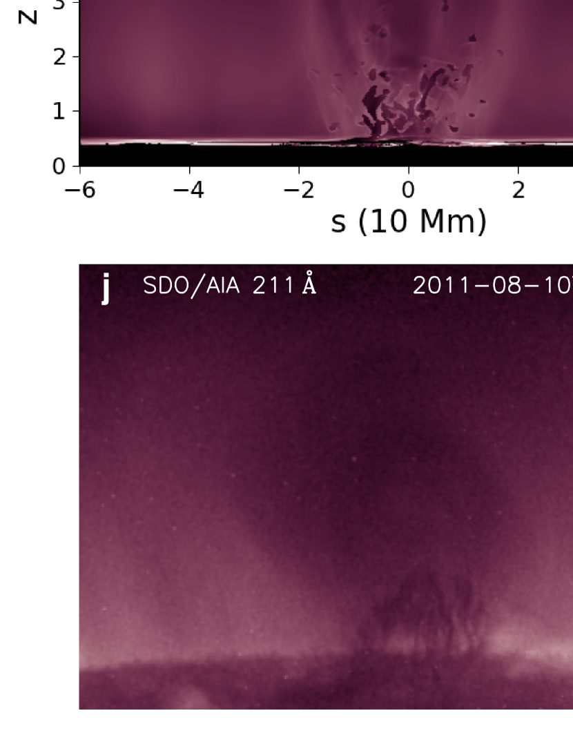
Figure 5: Synthetic EUV images of the forming prominence viewed along the axis of the prominence and comparison with observations. Synthetic SDO/AIA EUV images of the simulated prominence at wavebands 211, 171, and 304 Å, at time 40.1 minutes (a–c), 143.1 minutes (d–f), and 203.2 minutes (g–i) and SDO/AIA observations on a real prominence and its cavity (j–l). Supplementary Movie 1 shows the temporal evolution of these synthetic views.

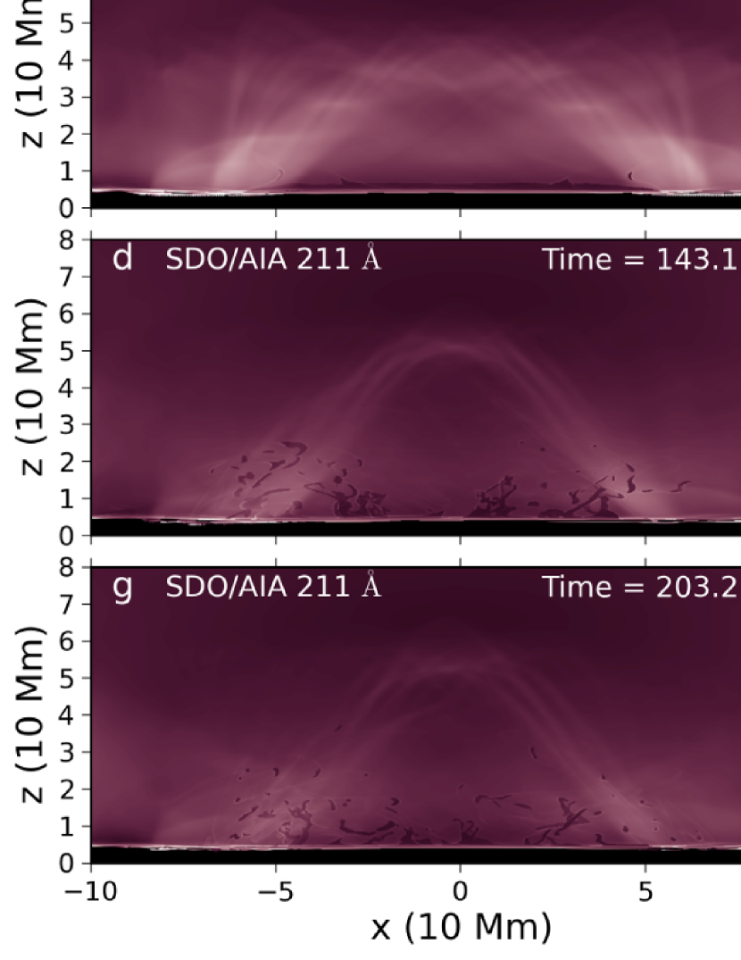
Figure 6: Synthetic EUV images of the forming prominence with the line of sight along the $y$-axis nearly perpendicular to the axis of the prominence. Synthetic SDO/AIA EUV images of the simulated prominence at wavebands 211, 171, and 304 Å, at time 40.1 minutes (a–c), 143.1 minutes (d–f), and 203.2 minutes (g–i). Supplementary Movie 2 shows the temporal evolution of these synthetic views.

References

- Antiochos et al. (1999) Antiochos, S. K., MacNeice, P. J., Spicer, D. S., & Klimchuk, J. A. 1999, ApJ, 512, 985
- Bak-Stȩślicka et al. (2013) Bak-Stȩślicka, U., Gibson, S. E., Fan, Y., Bethge, C., Forland, B., & Rachmeler, L. A. 2013, ApJ, 770, L28
- Berger et al. (2011) Berger, T., Testa, P., Hillier, A., Boerner, P., Low, B. C., Shibata, K., Schrijver, C., Tarbell, T., & Title, A. 2011, Nature, 472, 197
- Berger et al. (2012) Berger, T. E., Liu, W., & Low, B. C. 2012, ApJ, 758, L37
- Berger et al. (2008) Berger, T. E., Shine, R. A., Slater, G. L., Tarbell, T. D., Title, A. M., Okamoto, T. J., Ichimoto, K., Katsukawa, Y., Suematsu, Y., Tsuneta, S., Lites, B. W., & Shimizu, T. 2008, ApJ, 676, L89
- Berger et al. (2010) Berger, T. E., Slater, G., Hurlburt, N., Shine, R., Tarbell, T., Title, A., Lites, B. W., Okamoto, T. J., Ichimoto, K., Katsukawa, Y., Magara, T., Suematsu, Y., & Shimizu, T. 2010, ApJ, 716, 1288
- Blokland & Keppens (2011) Blokland, J. W. S. & Keppens, R. 2011, Astron. Astrophys., 532, A93
- Bommier et al. (1994) Bommier, V., Landi Degl’Innocenti, E., Leroy, J.-L., & Sahal-Brechot, S. 1994, Sol. Phys., 154, 231
- Chae et al. (2008) Chae, J., Ahn, K., Lim, E.-K., Choe, G. S., & Sakurai, T. 2008, ApJ, 689, L73
- Chiu & Hilton (1977) Chiu, Y. T. & Hilton, H. H. 1977, ApJ, 212, 873
- Dedner et al. (2002) Dedner, A., Kemm, F., Kröner, D., Munz, C.-D., Schnitzer, T., & Wesenberg, M. 2002, J. Comput. Phys., 175, 645
- Engvold (1976) Engvold, O. 1976, Sol. Phys., 49, 283
- Field (1965) Field, G. B. 1965, ApJ, 142, 531
- Fuller et al. (2008) Fuller, J., Gibson, S. E., de Toma, G., & Fan, Y. 2008, ApJ, 678, 515
- Gibson et al. (2010) Gibson, S. E., Kucera, T. A., Rastawicki, D., Dove, J., de Toma, G., Hao, J., Hill, S., Hudson, H. S., Marqué, C., McIntosh, P. S., Rachmeler, L., Reeves, K. K., Schmieder, B., Schmit, D. J., Seaton, D. B., Sterling, A. C., Tripathi, D., Williams, D. R., & Zhang, M. 2010, ApJ, 724, 1133
- Harten et al. (1983) Harten, A., Lax, P. D., & van Leer, B. 1983, SIAM Review, 25, 35
- Hillier et al. (2011) Hillier, A., Isobe, H., Shibata, K., & Berger, T. 2011, ApJ, 736, L1
- Hillier & van Ballegooijen (2013) Hillier, A. & van Ballegooijen, A. 2013, ApJ, 766, 126
- Kaneko & Yokoyama (2015) Kaneko, T. & Yokoyama, T. 2015, ApJ, 806, 115
- Karpen et al. (2001) Karpen, J. T., Antiochos, S. K., Hohensee, M., Klimchuk, J. A., & MacNeice, P. J. 2001, ApJ, 553, L85
- Keppens et al. (2012) Keppens, R., Meliani, Z., van Marle, A. J., Delmont, P., Vlasis, A., & van der Holst, B. 2012, J. Comput. Phys., 231, 718
- Keppens & Xia (2014) Keppens, R. & Xia, C. 2014, ApJ, 789, 22
- Keppens et al. (2015) Keppens, R., Xia, C., & Porth, O. 2015, ApJ, 806, L13
- Khomenko et al. (2014) Khomenko, E., Díaz, A., de Vicente, A., Collados, M., & Luna, M. 2014, Astron. Astrophys., 565, A45
- Kuperus & Raadu (1974) Kuperus, M. & Raadu, M. A. 1974, Astron. Astrophys., 31, 189
- Leighton (1964) Leighton, R. B. 1964, ApJ, 140, 1547
- Leroy et al. (1983) Leroy, J. L., Bommier, V., & Sahal-Brechot, S. 1983, Sol. Phys., 83, 135
- Liu et al. (2012) Liu, W., Berger, T. E., & Low, B. C. 2012, ApJ, 745, L21
- Low & Zhang (2004) Low, B. C. & Zhang, M. 2004, ApJ, 609, 1098
- Luna et al. (2012) Luna, M., Karpen, J. T., & DeVore, C. R. 2012, ApJ, 746, 30
- Meyer et al. (2012) Meyer, C. D., Balsara, D. S., & Aslam, T. D. 2012, Mon. Not. R. Astron. Soc., 422, 2102
- Orozco Suárez et al. (2014) Orozco Suárez, D., Asensio Ramos, A., & Trujillo Bueno, J. 2014, Astron. Astrophys., 566, A46
- Parker (1953) Parker, E. N. 1953, ApJ, 117, 431
- Porth et al. (2014) Porth, O., Xia, C., Hendrix, T., Moschou, S. P., & Keppens, R. 2014, ApJ, 214, 4
- Ryutova et al. (2010) Ryutova, M., Berger, T., Frank, Z., Tarbell, T., & Title, A. 2010, Sol. Phys., 267, 75
- Terradas et al. (2015) Terradas, J., Soler, R., Luna, M., Oliver, R., & Ballester, J. L. 2015, ApJ, 799, 94
- Townsend (2009) Townsend, R. H. D. 2009, ApJ, 181, 391
- Čada & Torrilhon (2009) Čada, M. & Torrilhon, M. 2009, J. Comput. Phys., 228, 4118
- van Ballegooijen & Martens (1989) van Ballegooijen, A. A. & Martens, P. C. H. 1989, ApJ, 343, 971
- Wang & Stenborg (2010) Wang, Y.-M. & Stenborg, G. 2010, ApJ, 719, L181
- Xia et al. (2012) Xia, C., Chen, P. F., & Keppens, R. 2012, ApJ, 748, L26
- Xia et al. (2011) Xia, C., Chen, P. F., Keppens, R., & van Marle, A. J. 2011, ApJ, 737, 27
- Xia et al. (2014a) Xia, C., Keppens, R., Antolin, P., & Porth, O. 2014a, ApJ, 792, L38
- Xia et al. (2014b) Xia, C., Keppens, R., & Guo, Y. 2014b, ApJ, 780, 130