Effective acoustic properties of a meta-material consisting of small Helmholtz resonators

Abstract

We investigate the acoustic properties of meta-materials that are inspired by sound-absorbing structures. We show that it is possible to construct meta-materials with frequency-dependent effective properties, with large and/or negative permittivities. Mathematically, we investigate solutions $u^{\varepsilon}:\Omega_{\varepsilon}\to\mathbb{R}$ to a Helmholtz equation in the limit $\varepsilon\to 0$ with the help of two-scale convergence. The domain $\Omega_{\varepsilon}$ is obtained by removing from an open set $\Omega\subset\mathbb{R}^{n}$ in a periodic fashion a large number (order $\varepsilon^{-n}$) of small resonators (order $\varepsilon$). The special properties of the meta-material are obtained through sub-scale structures in the perforations.

Keywords: Helmholtz equation, homogenization, resonance, perforated domain, frequency dependent effective properties

MSC: 78M40, 35P25, 35J05

1 Introduction

In this article, we are interested in the acoustic properties of a particular meta-material, inspired by sound absorbing structures. We define a complex geometry, consisting of many small cavities, and study the Helmholtz equation in this geometry. The acoustic properties of the meta-material are determined by the Helmholtz equation since the acoustic pressure $p$ of a time-harmonic sound wave of fixed frequency $\omega$ is of the form $p(x,t)=u(x)e^{i\omega t}$, where $u$ solves a Helmholtz equation.

In standard homogenization settings, nothing special can be expected concerning the acoustic properties of a meta-material (e.g. large or negative coefficients). Instead, in this contribution, we introduce a setting where the small inclusions are resonators and where the effective behavior of the meta-material introduces new features.

Let us describe these statements in a more mathematical language: We consider a domain $\Omega_{\varepsilon}\subset\mathbb{R}^{n}$, $n=2$ or $n=3$, which is obtained by removing small obstacles of typical size $\varepsilon>0$ from a domain $\Omega\subset\mathbb{R}^{n}$. For a fixed frequency $\omega\in\mathbb{R}$, we study solutions $u^{\varepsilon}\in H^{1}(\Omega_{\varepsilon})$ to the Helmholtz equation

$$\begin{split}-\Delta u^{\varepsilon}&=\omega^{2}u^{\varepsilon}\quad\,\text{ in }\Omega_{\varepsilon}\,,\\ \partial_{n}u^{\varepsilon}&=0\quad\quad\ \ \text{ on }\partial\Omega_{\varepsilon}\setminus\partial\Omega\,,\\ u^{\varepsilon}&=g\quad\quad\ \ \text{ on }\partial\Omega\,.\end{split}$$ (1.1)

The first boundary condition expresses that the obstacles are sound-hard (homogeneous Neumann condition, $n$ denotes the exterior normal at $\partial\Omega_{\varepsilon}$), the second boundary condition prescribes a pressure at the external boundary, $g\in H^{1}(\Omega)$ is responsible for the generation of a sound wave in the domain.

When $\Omega_{\varepsilon}$ is obtained from $\Omega$ by a standard periodic perforation procedure, then the homogenization of equation (1.1) is well-established. One finds an effective coefficient $A_{*}$ and a volume correction factor $\lambda\in(0,\infty)$ such that, for small $\varepsilon>0$, the solution $u^{\varepsilon}$ looks essentially like the solution $u^{*}$ of the effective equation $-\nabla\cdot(A_{*}\nabla u^{*})=\omega^{2}\lambda u^{*}$. In this effective system, neither $A^{*}$ nor $\lambda$ are frequency dependent.

In contrast to such a standard approach we investigate (1.1) for a domain $\Omega_{\varepsilon}$, where every single inclusion (perforation) has the shape of a small resonator. This is possible by introducing a three-scale problem: The macro-scale is $\mathrm{diam}(\Omega)=O(1)$, the micro-scale of the single inclusion is $O(\varepsilon)$, and the single inclusion contains a subscale feature of either size $O(\varepsilon^{2})$ (in dimension $n=3$) or $O(\varepsilon^{3})$ (in dimension $n=2$). In this three-scale domain $\Omega_{\varepsilon}$, the solutions $u^{\varepsilon}$ exhibit a more interesting behavior. We perform the homogenization procedure and find that, for small $\varepsilon>0$, the solution $u^{\varepsilon}$ to (1.1) looks essentially like the solution $v$ to the effective system

$$-\nabla\cdot\left(A_{*}\nabla v\right)=\omega^{2}\Lambda\,v\quad\text{ in }\Omega\,.$$ (1.2)

The form of this system is as in the standard homogenization setting, two effective coefficients $A_{*}$ and $\Lambda\in\mathbb{R}$ modify the original equation when describing the system with a macroscopic equation on $\Omega$. But, due to the more complex geometry, we obtain a parameter $\Lambda=\Lambda(\omega)$, which is frequency dependent. It can change sign and it can be arbitrarily large due to a resonance effect in the single cavity. The resonance frequency is given by the well-known formula for Helmholtz resonators, $\omega_{*}=\sqrt{A/(LV)}$, where the real numbers $A$, $L$, and $V$ characterize the geometric properties of the resonators (area of a channel cross section, length of the channel, volume of the resonator).

Usually, small inclusions correspond to a high resonance frequency, and not to some finite frequency $\omega_{*}$. But, as was shown in [30], a finite resonance frequency can be obtained when a singular structure is included in the geometry: We consider a setting where, in every periodicity cell $Y\subset\mathbb{R}^{n}$, a resonator region $R_{Y}\subset Y$ is separated from an exterior region $Q_{Y}\subset Y$ by the sound-hard obstacle $\Sigma_{Y}^{\varepsilon}\subset Y$, cp. Figure 1. But the separation is not complete, the obstacle leaves open a small channel that connects $R_{Y}$ and $Q_{Y}$. The scaling of the channel depends on the dimension. In two space dimensions ($n=2$), the relative scaling of the opening is $\varepsilon^{p}$ with $p=2$, hence the channel width of the single inclusion $\Sigma_{k}^{\varepsilon}\subset\Omega$ (where $k\in\mathbb{Z}^{n}$ is the index of the $k$-th inclusion) is of order $\varepsilon^{3}$. In dimension $n=3$ the exponent is $p=1$, the channel opening diameter of the single inclusion $\Sigma_{k}^{\varepsilon}\subset\Omega$ is therefore of order $\varepsilon^{2}$. In both cases, the scaling is such that the quantity $A_{\varepsilon}/(L_{\varepsilon}V_{\varepsilon})$ is of order $1$, where $A_{\varepsilon}$ is the channel opening, $L_{\varepsilon}$ is the channel length and $V_{\varepsilon}$ is the volume. Let us check this condition: For $n=2$ we have $A_{\varepsilon}/(L_{\varepsilon}V_{\varepsilon})\sim\varepsilon^{p+1}/(\varepsilon^{1}\varepsilon^{n})=1$, for $n=3$ we have $A_{\varepsilon}/(L_{\varepsilon}V_{\varepsilon})\sim(\varepsilon^{p+1})^{2}/(\varepsilon^{1}\varepsilon^{n})=1$.

1.1 Main result

We investigate a large domain $\Omega\subset\mathbb{R}^{n}$ that contains meta-material in some region $D\subset\Omega$. The single small resonator is denoted as $\Sigma_{k}^{\varepsilon}$, with $k\in\mathbb{Z}^{n}$ such that $\varepsilon\left(k+Y\right)\subset D$, where $Y:=(-\frac{1}{2},\frac{1}{2})^{n}$. The union of all resonators $\Sigma_{\varepsilon}=\bigcup_{k}\Sigma_{k}^{\varepsilon}\subset D$ defines the perforated domain $\Omega_{\varepsilon}:=\Omega\setminus\Sigma_{\varepsilon}$. In order to analyze the effect of the resonator region $D$, we study solutions $u^{\varepsilon}$ to the Helmholtz equation (1.1) and investigate their behavior inside and outside of $D$ in the limit $\varepsilon\to 0$.

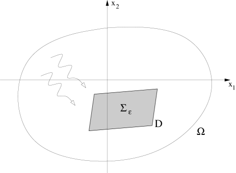
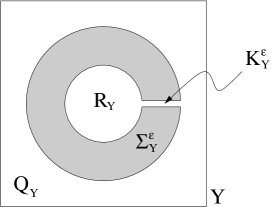
Figure 1: Sketch of the scattering problem. Left: The sub-region $D\subset\Omega$ contains the small Helmholtz resonators, given by $\Sigma_{\varepsilon}\subset D$. The number of resonators in the region $D$ is of order $\varepsilon^{-n}$. We are interested in the effective properties of the meta-material in $D$. Right: The microscopic geometry with the single resonator $R_{Y}$. The channel width inside $Y$ is of the order $\varepsilon^{p}$.

We derive an effective Helmholtz equation with the tool of two-scale convergence. Essentially, the effective system is given by (1.2). In this equation, the effective permittivity $\Lambda:\Omega\to\mathbb{R}$ is $\Lambda(x)=1$ for $x\in\Omega\setminus D$ (outside the region that contains the resonators) and $\Lambda(x)=\Lambda_{\mathrm{\tiny eff}}$ for $x\in D$, where the real number

$$\Lambda_{\mathrm{\tiny eff}}:=Q-\frac{A}{L}\left(\omega^{2}-\frac{A}{LV}\right)^{-1}$$ (1.3)

is determined by the positive real numbers $A$, $L$, $V$ and $Q$ which characterize the geometric properties of the resonators (area of a channel cross section, length of the channel, volume of the resonator, volume of the exterior), cf. Section 1.3 below. The number $\Lambda_{\mathrm{\tiny eff}}$ represents the permittivity of the effective medium. Due to resonance properties of $\Sigma_{Y}^{\varepsilon}$, it can be negative and it can be large in absolute value (with both signs). The resonance frequency $\omega_{*}=\sqrt{A/(LV)}$ is determined by the geometry.

The ellipticity matrix is $A_{*}(x)=\text{{\bf 1}}_{\mathbb{R}^{n}}$ for $x\in\Omega\setminus D$, whereas for $x\in D$ it is given as a cell problem integral:

$$\left(A_{*}\right)_{ij}(x):=\left(A_{\mathrm{\tiny eff}}\right)_{ij} :=\int_{Q_{Y}}\left[\delta_{ij}+\partial_{y_{i}}\chi_{j}(y)\right]\,dy\quad\text{ for }i,j\in\{1,...,n\}\,,$$ (1.4)

where $\delta_{ij}$ denotes the Kronecker Delta and $\chi_{j}$ is the solution to the cell problem (2.11). The set $Q_{Y}\subset Y$ is the part of the periodicity cell $Y$ that is exterior to the obstacle and $Q:=|Q_{Y}|$ is its volume.

Let us formulate here our main result in a condensed form. Theorem 1.1 characterizes the effective influence of the scattering region $D$ on waves in $\Omega$. Theorem 1.1 is a consequence of the stronger result in Theorem 3.1, which includes a characterization of $u^{\varepsilon}$ in $D$.

Theorem 1.1 (Effective Helmholtz equation).

Let $\Omega\subset\mathbb{R}^{n}$ be a domain and let $D\subset\Omega$ contain the obstacle set $\Sigma_{\varepsilon}\subset D$ as described in Section 1.3. Let $u^{\varepsilon}\in H^{1}(\Omega_{\varepsilon})$ be a sequence of solutions to (1.1) satisfying

$$\|u^{\varepsilon}\|_{L^{2}(\Omega_{\varepsilon})}\leq C\,.$$ (1.5)

Let $\Lambda_{\mathrm{\tiny eff}}$ and $\Lambda$ be defined by the algebraic relation (1.3), which uses the geometric constants $A,L,V,Q>0$. Let $A_{*}$ be defined by (1.4) with the help of cell problems. Let $v\in H^{1}(\Omega)$ be a solution to the effective Helmholtz equation

$$-\nabla\cdot\left(A_{*}\nabla v\right) =\omega^{2}\Lambda\,v\quad\text{ in }\Omega\,,$$ (1.6)

$$v =g\quad\quad\quad\text{ on }\partial\Omega\,.$$ (1.7)

If the solution $v$ to the effective system is unique, then there holds

$$u^{\varepsilon}|_{\Omega\setminus D}\to v|_{\Omega\setminus D}\quad\text{ in }L^{2}(\Omega\setminus D)\,.$$ (1.8)

Remark 1.2.

For almost every $\omega\in\mathbb{R}$ the solution to (1.6)-(1.7) is unique, since the generalized Eigenvalue-problem (1.6) has a discrete set of Eigenvalues $\omega^{2}$.

The result of Theorem 1.1 yields that the field $u^{\varepsilon}$ is determined outside the resonator region $D$ by the effective system (1.6)–(1.7). Inside $D$, the solutions $u^{\varepsilon}$ are oscillatory due to the micro-structure. We describe the two-scale limit of $u^{\varepsilon}$ in $D$ in Subsection 1.4.

1.2 Literature

Homogenization theory is concerned with the derivation of effective equations. The most elementary task is to consider a sequence $u^{\varepsilon}$ of solutions to a family of partial differential equations that contains a small parameter $\varepsilon$, very often the periodicity of the geometry or the periodicity of a coefficient. The goal is to find an equation that characterizes the weak limit $u^{*}$ of the sequence $u^{\varepsilon}$. Our result is of that form. The general theory has origins in [29] and it was greatly simplified by introducing the notion of two-scale convergence [1, 26]. The theory was later extended in several directions, e.g. to stochastic problems [21], to problems with multiple scales [2], and to problems with measure valued limits [8, 14].

Perforated media. Our result treats perforated media in the sense that an equation with constant coefficients is considered on a domain $\Omega_{\varepsilon}$ which is obtained by removing many small subdomains from a macroscopic domain $\Omega$. A simple boundary condition is imposed on the boundary $\partial\Omega_{\varepsilon}\setminus\partial\Omega$. Perforated media have been studied with Dirichlet boundary conditions in [16] and with Neumann boundary conditions in [17], the scattering problem has been analyzed in [15]. For perforations along a lower dimensional manifold see e.g. [19]. Periodically perforated domains can also be treated with the tool of two-scale convergence, which shortens the proofs of some of the original results. The difference between our result and those mentioned above is that we introduce a sub-scale structure in the perforation to allow for resonances. This leads to more interesting terms in the effective equation.

Resonances in Maxwell’s equations. Resonances in the single periodicity cell can create interesting effects in the homogenization limit. One of the fascinating examples is the construction of negative index materials for light as suggested in [27, 28] with its possible applications to cloaking (see [23] and the references therein). The meta-material for the Maxwell’s equations has qualitatively new features, namely a negative effective permittivity and a negative effective permeability. The astonishing properties of such a material had been anticipated in [31], but the mathematical analysis of negative index meta-materials is much younger. Model equations have been studied in [22], non-rigorous results appeared in [13, 20]. The mathematical theory that confirmed negative effective permeability appeared in [11, 24] for metals and in [7] for dielectrics. The full result on the negative effective index meta-material can be found in [25].

Generation of resonances. At first sight, a resonance effect in a structure of order $\varepsilon$ seems impossible when the frequency $\omega$ is kept fixed: One expects that an object of order $\varepsilon$ has a resonance at wave-length of order $\varepsilon$ and hence a resonance frequency of order $\varepsilon^{-1}$. Indeed, in order to obtain interesting features in the limit $\varepsilon\to 0$, one has to introduce some singular behavior of the micro-structure.

(a) Large contrast. The simplest setting uses a large contrast, e.g. a parameter $a_{\varepsilon}$ that is of order $1$ outside the structure and $\varepsilon^{2}$ in the structure [7, 12, 13, 25]. In many cases, the large contrast must be combined with one of the features (b)-(d) below.

(b) Fibers. Interesting effects within the framework of homogenization can be obtained when fibers are present in the structure [4, 5, 6, 13]. On the one hand a fiber can be regarded as a classical periodic micro-structure ($\varepsilon$-periodic in each direction). On the other hand, the exterior of the fiber (in the single cell) is not a simply connected set, which makes some standard two-scale limit characterizations impossible. Other effects are related to the fact that the length of a single fiber is of order $O(1)$. For implications in Maxwell equations see e.g. [9, 10, 13, 25].

(c) Split rings. More complicated is the three-dimensional construction of a split ring: For $\varepsilon>0$, the ring is simply connected, but the slit closes in the limit $\varepsilon\to 0$ such that the limiting object is no longer simply connected. This change of topology is exploited in [11, 24].

(d) Disconnected subregions. In the work at hand we use a different construction, based on the Helmholtz resonator that has been studied mathematically in [30]. Again, a topological effect plays a role: Every cell has an interior part $R_{Y}$ (the resonator) and an exterior part $Q_{Y}$. For every $\varepsilon>0$, the two subdomains are connected by a thin channel, but since the channel gets thinner and thinner, the limiting object for $\varepsilon\to 0$ is no longer connected, it has the two disconnected components $R_{Y}$ and $Q_{Y}$.

In both settings (c) and (d) it is the change of the topology that makes the resonance in the small object at finite frequency possible. We note that the analysis of spectral properties in perforated domains require other methods if the low- and high-frequency parts of the spectrum are studied separately, see [3, 21, 32].

1.3 Geometry

Let $\Omega\subset\mathbb{R}^{n}$ be open and bounded and let $D\subset\Omega$ be an open set with Lipschitz boundary such that $\bar{D}\subset\Omega$. The set $D$ contains the periodic perforations, it is the scatterer in the effective equations.

Microscopic geometry. We start the construction from the periodicity cube $Y:=(-\frac{1}{2},\frac{1}{2})^{n}$. Since we will always impose periodicity conditions on the cube $Y$, we may identify it with the torus $\mathbb{T}^{n}$. We assume that $Y$ is the disjoint union

$$Y=R_{Y}\cup\bar{\Sigma}_{Y}\cup Q_{Y}\,,$$

each of the three sets $R_{Y},\Sigma_{Y},Q_{Y}$ is open and connected with Lipschitz boundary, $\bar{R}_{Y},\bar{\Sigma}_{Y}\subset(-\frac{1}{2},\frac{1}{2})^{n}$ do not touch the boundary, and $R_{Y}\cup Q_{Y}$ is not connected, see Figure 1.

Channel construction. The channel is constructed starting from a one-dimensional line-segment $\Gamma_{Y}\subset\Sigma_{Y}$ that connects $\partial R_{Y}$ with $\partial Q_{Y}$. We may write the segment with its tangential vector $\tau_{\Gamma_{Y}}\in\mathbb{R}^{n}$ as $\Gamma_{Y}=\{\gamma_{0}+t\tau_{\Gamma_{Y}}:t\in(0,L)\}$ with $L$ denoting the length of the segment. For ease of notation we assume in the following that the line segment has the tangential vector $\tau_{\Gamma_{Y}}=e_{1}$ and that $\Gamma_{Y}\subset\mathbb{R}\times\{0\}\subset\mathbb{R}^{n}$. In this case, we have $\gamma_{0}=(y_{R},0)$ and $\Gamma_{Y}=(y_{R},y_{Q})\times\{0\}$ with $y_{Q}:=y_{R}+L<1/2$.

For technical reasons in the study of the asymptotic behavior of cell solutions, we assume that the boundaries $\partial R_{Y}$ and $\partial Q_{Y}$ are flat in the vicinity of $(y_{R},0)$ and $(y_{Q},0)$: For some $\delta>0$ there holds $\partial R_{Y}\cap B_{\delta}((y_{R},0))\subset\{y_{R}\}\times\mathbb{R}^{n-1}$ and similarly for $\partial Q_{Y}$.

We now construct the channel as $K_{Y}^{\varepsilon}:=B_{\alpha\varepsilon^{p}}(\Gamma_{Y})\cap\Sigma_{Y}$, where $\alpha>0$ is fixed and $B_{\alpha\varepsilon^{p}}$ denotes the generalized ball around a set. In our simplified setting, the channel is the cylinder $K_{Y}^{\varepsilon}=(y_{R},y_{Q})\times B^{n-1}_{\alpha\varepsilon^{p}}(0)\subset Y$, where $B^{n-1}_{\alpha\varepsilon^{p}}(0)$ is the $n-1$-dimensional ball with radius ${\alpha\varepsilon^{p}}$. The Helmholtz resonator $\Sigma_{Y}^{\varepsilon}$ is defined as

$$\Sigma_{Y}^{\varepsilon}:=\Sigma_{Y}\setminus\bar{K}_{Y}^{\varepsilon}=Y\setminus\left(\bar{R}_{Y}\cup\bar{K}_{Y}^{\varepsilon}\cup\bar{Q}_{Y}\right).$$ (1.9)

In the following, three geometric quantities will be crucial: (i) The length $L$ of the channel. (ii) The relative cross section area $A$ of the channel, $A=2\alpha$ for $n=2$ and $A=\alpha^{2}\pi$ for $n=3$. (iii) The volume $V=|R_{Y}|$ of the inner connected component $R_{Y}$. We will see that in the effective equation resonances appear at frequencies $\omega^{2}$ that are close to the ratio $A/(LV)$.

Macroscopic geometry. In order to define the domain $\Omega_{\varepsilon}$, we use indices $k\in\mathbb{Z}^{n}$ and shifted small cubes $Y_{k}^{\varepsilon}:=\varepsilon(k+Y)$. We denote by $\mathcal{K}:=\{k\in\mathbb{Z}^{n}\,|\,Y_{k}^{\varepsilon}\subset D\}$ the set of indices $k$ such that the small cube $Y_{k}^{\varepsilon}$ is contained in $D$. Here and in the following, in summations or unions over $k$, the index $k$ takes all values in the index set $\mathcal{K}$. The number of relevant indices is of the order $|\mathcal{K}|=O(\varepsilon^{-n})$.

Using the local subset $\Sigma_{Y}^{\varepsilon}\subset Y$ we define the union $\Sigma_{\varepsilon}$ of scaled obstacles and the perforated domain $\Omega_{\varepsilon}$ by

$$\Sigma_{\varepsilon}:=\bigcup_{k\in\mathcal{K}}\Sigma_{k}^{\varepsilon}:=\bigcup_{k\in\mathcal{K}}\varepsilon(k+\Sigma^{\varepsilon}_{Y})\,,\quad\quad\Omega_{\varepsilon}:=\Omega\setminus\bar{\Sigma}_{\varepsilon}\,.$$ (1.10)

Also the other microscopic quantities have their counterpart in the macroscopic domain: The union $K_{\varepsilon}$ of the channels, the union $Q_{\varepsilon}$ of exterior components and the union $R_{\varepsilon}$ of interior components are

$$K_{\varepsilon}:=\bigcup_{k\in\mathcal{K}}\varepsilon(k+K_{Y}^{\varepsilon})\,,\quad Q_{\varepsilon}:=\bigcup_{k\in\mathcal{K}}\varepsilon(k+Q_{Y})\,,\quad R_{\varepsilon}:=\bigcup_{k\in\mathcal{K}}\varepsilon(k+R_{Y})\,.$$ (1.11)

1.4 Characterization of solutions in $D$

Outside the scatterer region $D$, the function $v$ of the effective system (1.6)–(1.7) is the weak limit of $u^{\varepsilon}$. In the following, we want to describe the meaning of $v$ in the scatterer region $D$.

If we denote by $\tilde{u^{\varepsilon}}\in L^{2}(\Omega)$ the trivial extension of $u^{\varepsilon}$ by zero, then the uniform bound (1.5) implies the existence of a subsequence and of a two-scale limit $u_{0}=u_{0}(x,y)$ such that $\tilde{u^{\varepsilon}}\stackrel{{\scriptstyle 2s}}{{\rightharpoonup}}u_{0}$ (for the definition of two-scale convergence we refer to [1]). Proposition 2.1 below yields that the two-scale limit for $x\in D$ is of the form

$$\begin{split}u_{0}(x,y)=\begin{cases}v(x)&\;\;\text{ for }y\in Q_{Y},\\ w(x)&\;\;\text{ for }y\in R_{Y},\\ 0&\;\;\text{ for }y\in\Sigma_{Y}.\end{cases}\end{split}$$ (1.12)

This characterization clarifies the meaning of $v$. Outside the perforated region $D\subset\Omega$, there is no micro-structure and the sequence $u^{\varepsilon}$ converges strongly to $v$. Instead, for $x\in D$, the function $v$ describes the value of $u_{0}$ in the exterior $Q_{Y}$ of the Helmholtz resonator. Outside $D$, the limit function $v$ is comparable to $u^{\varepsilon}$, while inside $D$ the function $v$ stands for the values of $u^{\varepsilon}$ outside the scatterers. This fits with the result $v\in H^{1}(\Omega)$ from Lemma 2.2 below: It is the function $v$ that has a weak continuity property across the boundaries of $D$.

2 Two-scale limits

We will always work with the assumption that the sequence $u^{\varepsilon}$ is uniformly bounded in $L^{2}(\Omega_{\varepsilon})$ as demanded in (1.5). We remark that (1.5) implies also a uniform $H^{1}$-bound,

$$\|u^{\varepsilon}\|_{H^{1}(\Omega_{\varepsilon})}\leq C$$ (2.1)

for some $\varepsilon$-independent constant $C>0$. Since the boundary values are given by $g\in H^{1}(\Omega)$ and since the domain $\Omega$ is bounded, the estimate (2.1) follows immediately from (1.5) by testing (1.1) with the solution $u^{\varepsilon}$.

In this section we derive Relation (1.12) for the two-scale limit $u_{0}$. Moreover, we provide a characterization for the two-scale limit of the gradients $\nabla u^{\varepsilon}$.

2.1 The two-scale limit $u_{0}$

The following proposition provides a first characterization of $u_{0}$. We use the sequence $\tilde{u^{\varepsilon}}\in L^{2}(\Omega)$ of trivial extensions of $u^{\varepsilon}$ (obtained by setting $\tilde{u^{\varepsilon}}(x):=0$ for $x\in\Sigma_{\varepsilon}$).

Proposition 2.1 (The two-scale limit $u_{0}$).

Let $u^{\varepsilon}\in H^{1}(\Omega_{\varepsilon})$ be a sequence of solutions to (1.1). We assume that the sequence satisfies the uniform bound (1.5) and that $\tilde{u^{\varepsilon}}\in L^{2}(\Omega)$ converges in two scales to some limit function $u_{0}\in L^{2}(\Omega\times Y)$. Then there exist $v\in L^{2}(\Omega)$ and $w\in L^{2}(D)$ such that

1. For $x\in\Omega\setminus D$ one has $u_{0}(x,y)=v(x)$.

2. For $x\in D$ one has

   $$\begin{split}u_{0}(x,y)=\begin{cases}v(x)&\;\;\text{ for }y\in Q_{Y},\\ w(x)&\;\;\text{ for }y\in R_{Y},\\ 0&\;\;\text{ for }y\in\Sigma_{Y}.\end{cases}\end{split}$$ (2.2)

Proof.

We start with the characterization of $u_{0}(x,y)$ for $(x,y)\in D\times\Sigma_{Y}$. Therefore, we consider localized test functions $\varphi_{\varepsilon}(x):=\theta(x)\Psi\left(\frac{x}{\varepsilon}\right)$ with $\theta\in C_{c}^{\infty}(D)$ and $\Psi\in C^{\infty}(Y)$ with $\text{supp}(\Psi)\subset\Sigma_{Y}$. On the one hand we find, exploiting the two-scale convergence of $\tilde{u}^{\varepsilon}$,

$$\int_{\Omega}\tilde{u^{\varepsilon}}(x)\varphi_{\varepsilon}(x)\,dx\rightarrow\int_{D}\theta(x)\int_{\Sigma_{Y}}u_{0}(x,y)\Psi(y)\,dy\,dx\,.$$

On the other hand one obtains, using the fact that $\text{supp}(\varphi_{\varepsilon})\subset(\Sigma_{\varepsilon}\cup\bar{K}_{\varepsilon})$, the definition of $\tilde{u^{\varepsilon}}$, the $L^{2}(\Omega)$-bound for $\tilde{u^{\varepsilon}}$ and the vanishing volume fraction of the channels $K_{\varepsilon}$,

$$\int_{\Omega}\tilde{u^{\varepsilon}}(x)\varphi_{\varepsilon}(x)\,dx=\int_{K_{\varepsilon}}\tilde{u^{\varepsilon}}(x)\varphi_{\varepsilon}(x)\,dx\rightarrow 0\,.$$

Since the test functions were arbitrary, we conclude $u_{0}(x,y)=0$ for $(x,y)\in D\times\Sigma_{Y}$.

We next show that $u_{0}(x,y)$ is independent of $y$ for $(x,y)\in D\times Q_{Y}$. As before we consider localized test functions $\varphi_{\varepsilon}(x):=\theta(x)\Psi\left(\frac{x}{\varepsilon}\right)$ with $\theta\in C_{c}^{\infty}(D)$ and $\Psi\in C^{\infty}_{per}(Y,\mathbb{R}^{n})$ with $\text{supp}(\Psi)\subset Q_{Y}$. Multiplying $\nabla u^{\varepsilon}$ by $\varepsilon\varphi_{\varepsilon}$ and integrating by parts gives

$$\varepsilon\int_{\Omega_{\varepsilon}}\nabla u^{\varepsilon}(x)\cdot\varphi_{\varepsilon}(x)\,dx=-\int_{\Omega_{\varepsilon}}u^{\varepsilon}(x)\left[(\nabla_{y}\cdot\Psi)\left(\frac{x}{\varepsilon}\right)\theta(x)+\varepsilon\Psi\left(\frac{x}{\varepsilon}\right)\cdot\nabla_{x}\theta(x)\right]\,dx\,.$$ (2.3)

Note that no boundary terms appear due to the compact support of $\theta$ and $\Psi$. We can now pass to the limit $\varepsilon\rightarrow 0$. Due to the uniform $L^{2}$-bound of $\nabla u^{\varepsilon}$, cf. (2.1), the left hand side of (2.3) vanishes in the limit as $\varepsilon\rightarrow 0$. On the right hand side we exploit the two-scale convergence of $\tilde{u^{\varepsilon}}$ to find

$$\int_{\Omega_{\varepsilon}}u^{\varepsilon}(x)\left[(\nabla_{y}\cdot\Psi)\left(\frac{x}{\varepsilon}\right)\theta(x)+\varepsilon\Psi\left(\frac{x}{\varepsilon}\right)\cdot\nabla_{x}\theta(x)\right]\,dx$$

$$\qquad=\int_{\Omega}\tilde{u^{\varepsilon}}(x)\left[(\nabla_{y}\cdot\Psi)\left(\frac{x}{\varepsilon}\right)\theta(x)+\varepsilon\Psi\left(\frac{x}{\varepsilon}\right)\cdot\nabla_{x}\theta(x)\right]\,dx$$

$$\qquad\stackrel{{\scriptstyle\varepsilon\rightarrow 0}}{{\rightarrow}}\int_{D}\theta(x)\int_{Q_{Y}}u_{0}(x,y)(\nabla_{y}\cdot\Psi)(y)\,dy\,dx\,.$$

Since the test functions $\theta,\Psi$ were arbitrary, this implies that $\nabla_{y}u_{0}(x,.)=0$ in the sense of distributions in $Q_{Y}$ for almost every $x\in D$. Therefore $u_{0}$ does not depend on $y$ for $(x,y)\in D\times Q_{Y}$. We may therefore write $u_{0}(x,y)=v(x)$ for some $v\in L^{2}(D)$.

For the domains $(\Omega\setminus D)\times Y$ and $D\times R_{Y}$ one proceeds analogously to show that $u_{0}(x,.)$ does not depend on $y$. ∎

2.2 Two-scale convergence of the gradients

Due to the uniform bound (2.1) we can find also a two-scale limit of the sequence $\nabla u^{\varepsilon}$ (upon extending by zero). The subsequent Lemma provides a first characterization of the two-scale limit. We use the space $H_{per}^{1}(Q_{Y})$ of those functions in $H^{1}(Q_{Y})$ for which also their periodic extension to $\mathbb{R}^{n}$ is locally of class $H^{1}$.

Lemma 2.2.

Let $u^{\varepsilon}\in H^{1}(\Omega_{\varepsilon})$ be a sequence of solutions to (1.1) that satisfies the uniform bound (1.5). Let $\xi^{\varepsilon}\in L^{2}(\Omega;\mathbb{R}^{n})$ be the trivial extension of $\nabla u^{\varepsilon}$ by zero and let $v$ be the exterior field of Proposition 2.1. We assume that $\xi^{\varepsilon}$ converges in two scales to some limit function $\xi_{0}\in L^{2}(\Omega\times Y)^{n}$. Then the following holds:

1. The exterior field $v$ is of class $H^{1}(\Omega)$.

2. For $x\in\Omega\setminus D$ one has $\xi_{0}(x,y)=\nabla_{x}v(x)$.

3. There exists $v_{1}\in L^{2}(D;H_{per}^{1}(Q_{Y}))$ such that for $x\in D$ one has

   $$\begin{split}\xi_{0}(x,y)=\begin{cases}\nabla_{x}v(x)+\nabla_{y}v_{1}(x,y)&\;\;\text{ for }y\in Q_{Y},\\ 0&\;\;\text{ for }y\in R_{Y}\cup\Sigma_{Y}.\end{cases}\end{split}$$ (2.4)

We note that the lemma implies for the interior of the resonators

$$\nabla u^{\varepsilon}\,{\bf 1}_{R_{\varepsilon}}\stackrel{{\scriptstyle 2s}}{{\rightharpoonup}}0\quad\text{ as }\varepsilon\rightarrow 0\,.$$ (2.5)

Proof.

Step 1. Regularity of $v$. We consider the domain $\hat{\Omega}_{\varepsilon}:=\Omega\setminus(\bar{\Sigma}_{\varepsilon}\cup\bar{K}_{\varepsilon}\cup\bar{R}_{\varepsilon})$, which is obtained from $\Omega$ by removing the union of obstacles $\Sigma_{\varepsilon}$, slits $K_{\varepsilon}$ and interior regions $R_{\varepsilon}$. In particular, the perforation of $\hat{\Omega}_{\varepsilon}$ in each periodicity cell is a Lipschitz domain without substructure. We construct a sequence $\hat{v}^{\varepsilon}\in H^{1}(\Omega)$ by setting $\hat{v}^{\varepsilon}:=u^{\varepsilon}$ in $\hat{\Omega}_{\varepsilon}$ and extending to $\Omega$. Actually, it is well known that there exists a family of extension operators $\mathcal{P}_{\varepsilon}:H^{1}(\hat{\Omega}_{\varepsilon})\rightarrow H^{1}(\Omega)$ such that

$$\left\|\mathcal{P}_{\varepsilon}u^{\varepsilon}\right\|_{H^{1}(\Omega)}\leq C\|u^{\varepsilon}\|_{H^{1}(\hat{\Omega}_{\varepsilon})}$$

for some $C>0$ independent of $\varepsilon$, see [18], Chapter 1. Essentially, $\mathcal{P}_{\varepsilon}$ is defined by using in each perforation the harmonic extension of the boundary values. Hence, $\hat{v}^{\varepsilon}:=\mathcal{P}_{\varepsilon}u^{\varepsilon}$ is uniformly bounded in $H^{1}(\Omega)$. We therefore find, up to a subsequence, a limit function $\hat{v}\in H^{1}(\Omega)$ such that $\hat{v}^{\varepsilon}$ converges in two scales and strongly in $L^{2}(\Omega)$ to the ($y$-independent) function $\hat{v}=\hat{v}(x)$.

Since $\hat{v}^{\varepsilon}=u^{\varepsilon}$ in $\hat{\Omega}_{\varepsilon}$, the strong limit $\hat{v}$ coincides with the two-scale limit of $u^{\varepsilon}$ in the exterior of the resonators, i.e. $\hat{v}=v$. This proves $v\in H^{1}(\Omega)$.

Step 2. Characterization outside $D$. Outside of $D$, the elliptic equation for $u^{\varepsilon}$ implies that the solution sequence is locally $H^{2}$-bounded. Therefore, the distributional convergence $\nabla u^{\varepsilon}\to\nabla v$ is locally a strong $L^{2}$-convergence. In this case the two-scale limit of gradients coincides with the strong limit.

Step 3. Characterization in $D$: The case $y\in Q_{Y}\cup\Sigma_{Y}$. Concerning the characterization for $(x,y)\in D\times Q_{Y}$ we refer to a standard argument, which can be found e.g. in the proof of Theorem 2.9 in [1]. It provides the existence of a two-scale function $v_{1}\in L^{2}(D;H_{per}^{1}(Q_{Y}))$ such that

$$\xi_{0}(x,y)=\nabla_{x}v(x)+\nabla_{y}v_{1}(x,y)\quad\text{for }(x,y)\in D\times Q_{Y}.$$ (2.6)

We emphasize that characterization (2.6) heavily relies on the fact that the union of exterior domains is connected.

The claim for $y\in\Sigma_{Y}$ follows as in the proof of Proposition 2.1: We exploit the vanishing volume fraction of the channels and the uniform bound for $\nabla u^{\varepsilon}$.

Step 4. Characterization in $D$: The case $y\in R_{Y}$. For $y\in R_{Y}$ we argue as follows: Let $\theta\in C_{c}^{\infty}(D)$ and $\Psi\in C_{c}^{\infty}(R_{Y},\mathbb{R}^{n})$ be arbitrary. In three space dimensions, $n=3$, we exploit the relation $\mathrm{curl}(\nabla u^{\varepsilon})=0$, while in two space dimensions the $\mathrm{curl}$-operator has to be replaced by a rotated divergence. In the following, we perform the calculations only for $n=3$. Multiplying the identity $\mathrm{curl}(\nabla u^{\varepsilon})=0$ with $\varepsilon\,\theta(x)\Psi\left(\frac{x}{\varepsilon}\right)$ and integrating by parts one finds

$$0 =\int_{\Omega_{\varepsilon}}\mathrm{curl}(\nabla u^{\varepsilon})(x)\cdot\varepsilon\Psi\left(\frac{x}{\varepsilon}\right)\theta(x)\,dx$$

$$=\int_{\Omega_{\varepsilon}}\nabla u^{\varepsilon}(x)\cdot\left[\mathrm{curl}_{y}\Psi\left(\frac{x}{\varepsilon}\right)\theta(x)-\varepsilon\Psi\left(\frac{x}{\varepsilon}\right)\wedge\nabla_{x}\theta(x)\right]\,dx$$

$$\stackrel{{\scriptstyle\varepsilon\rightarrow 0}}{{\rightarrow}}\int_{D}\int_{R_{Y}}\xi_{0}(x,y)\cdot\mathrm{curl}_{y}\Psi(y)\theta(x)\,dy\,dx\,.$$

Since $\theta\in C_{c}^{\infty}(D)$ was arbitrary we conclude that for a.e. $x\in D$ and every $\Psi\in C_{c}^{\infty}(R_{Y},\mathbb{R}^{3})$ there holds

$$\int_{R_{Y}}\xi_{0}(x,y)\cdot\mathrm{curl}_{y}\Psi(y)\,dy=0\,.$$

We obtained that the (distributional) curl of $\xi_{0}$ vanishes. Since the interior domain $R_{Y}$ is simply connected, $\xi_{0}(x,\cdot)$ must be a gradient: There exists a potential $w_{1}\in L^{2}(D;H^{1}(R_{Y}))$ such that $\xi_{0}(x,\cdot)=\nabla_{y}w_{1}(x,\cdot)$ for a.e. $x\in D$. With an analogous calculation the same result can be obtained also in two space dimensions, $n=2$.

We next show that $w_{1}(x,\cdot)$ is constant for a.e. $x\in D$. This implies $\xi_{0}(x,y)=\nabla_{y}w_{1}(x,y)=0$; with that, the lemma is proven.

We consider microscopic test-functions $\psi\in C^{\infty}(\bar{R}_{Y})$ with vanishing values at the entrance of the channel. More precisely, denoting by $\Gamma_{Y}^{\varepsilon,R}:=\bar{R}_{Y}\cap\bar{K}_{Y}^{\varepsilon}=\{y_{R}\}\times\overline{B^{n-1}_{\alpha\varepsilon^{p}}(0)}$ the interface between $R_{Y}$ and the channel $K_{Y}^{\varepsilon}$ we define, for $\delta>0$ fixed, the set

$$\mathcal{A}_{\delta}(R_{Y}):=\left\{\psi\in C^{\infty}(\bar{R}_{Y})\,|\,\psi=0\,\text{ on }\{y_{R}\}\times B_{\delta}^{n-1}(0)\right\}.$$ (2.7)

Note that for $\delta>0$ fixed and $\varepsilon$ sufficiently small each $\psi_{\delta}\in\mathcal{A}_{\delta}(R_{Y})$ satisfies $\psi_{\delta}=0$ on $\Gamma_{Y}^{\varepsilon,R}$. Let now $\theta\in C_{c}^{\infty}(D)$ and $\psi_{\delta}\in\mathcal{A}_{\delta}(R_{Y})$ be arbitrary. We multiply $-\Delta u^{\varepsilon}$ with $\varepsilon\,\theta(x)\psi_{\delta}\left(\frac{x}{\varepsilon}\right)$ and integrate by parts to find

$$\begin{split}&\varepsilon\int_{\Omega_{\varepsilon}}(-\Delta u^{\varepsilon})(x)\,\theta(x)\psi_{\delta}\left(\frac{x}{\varepsilon}\right)\,dx\\ &\qquad=\int_{R_{\varepsilon}}\nabla u^{\varepsilon}\cdot\left[\varepsilon\nabla_{x}\theta(x)\psi_{\delta}\left(\frac{x}{\varepsilon}\right)+\theta(x)\nabla_{y}\psi_{\delta}\left(\frac{x}{\varepsilon}\right)\right]\,dx\,.\end{split}$$ (2.8)

Note that no boundary terms appear due to the Neumann boundary conditions of $u^{\varepsilon}$ and the fact that the test function $\Psi_{\delta}$ vanishes at the interface between $R_{Y}$ and the channel. We next pass to the limit in (LABEL:eq:testnabla). Exploiting that $\Delta u^{\varepsilon}$ is uniformly bounded in $L^{2}(\Omega_{\varepsilon})$ we find that the left hand side of (LABEL:eq:testnabla) vanishes in the limit as $\varepsilon\rightarrow 0$. On the right hand side we use the uniform boundedness of $\nabla u^{\varepsilon}$ to conclude that the first term vanishes in the limit, while for the second term we obtain

$$\int_{\Omega_{\varepsilon}}\nabla u^{\varepsilon}\cdot\theta(x)\nabla_{y}\psi_{\delta}\left(\frac{x}{\varepsilon}\right)\,dx \stackrel{{\scriptstyle\varepsilon\rightarrow 0}}{{\rightarrow}}\int_{D}\int_{R_{Y}}\xi_{0}(x,y)\cdot\nabla_{y}\psi_{\delta}(y)\theta(x)\,dy\,dx$$

$$=\int_{D}\int_{R_{Y}}\nabla_{y}w_{1}(x,y)\cdot\nabla_{y}\psi_{\delta}(y)\theta(x)\,dy\,dx\,.$$

In the last line we used the characterization $\xi_{0}(x,y)=\nabla_{y}w_{1}(x,y)$. Since $\theta$ was arbitrary we conclude, for a.e. $x\in D$ and every test function $\psi_{\delta}(y)\in\mathcal{A}_{\delta}(R_{Y})$,

$$\int_{R_{Y}}\nabla_{y}w_{1}(x,y)\cdot\nabla_{y}\psi_{\delta}(y)\,dy=0\,.$$ (2.9)

In the above equality the test functions $\psi_{\delta}$ are restricted to the set $\mathcal{A}_{\delta}(R_{Y})$. We claim that (2.9) holds for all functions $\psi\in C^{\infty}(\bar{R}_{Y})$. Indeed, in the limit $\delta\rightarrow 0$ the set $\{y_{R}\}\times B^{n-1}_{\delta}(0)$ shrinks to a set of vanishing $H^{1}$-capacity. In particular, for every $\psi\in C^{\infty}(\bar{R}_{Y})$ there exists an approximating sequence $\psi_{\delta}\in\mathcal{A}_{\delta}(R_{Y})$ with $\psi_{\delta}\rightarrow\psi$ in $H^{1}(R_{Y})$ as $\delta\rightarrow 0$. We therefore conclude that for every $\psi\in C^{\infty}(\bar{R}_{Y})$

$$\int_{R_{Y}}\nabla_{y}w_{1}(x,y)\cdot\nabla_{y}\psi(y)\,dy=0\,.$$

We obtain that $w_{1}(x,\cdot)$ is a solution to

$$-\Delta_{y}w_{1}(x,\cdot) =0\quad\text{ in }R_{Y},$$

$$\partial_{n}w_{1}(x,\cdot) =0\quad\text{ on }\partial R_{Y}\,.$$

All solutions to this elliptic problem are constant functions, as can be shown by testing with $w_{1}$. We obtain $\xi_{0}(x,y)=\nabla_{y}w_{1}(x,y)=0$ for $(x,y)\in D\times R_{Y}$, which concludes the proof. ∎

In the next lemma we relate, via cell problems, the two-scale function $v_{1}$ (the exterior two-scale corrector) to the field $v$ (which represents average values outside the resonators). The procedure follows the standard arguments, our interest is to show rigorously that the channels do not affect the equations for the exterior corrector function $v_{1}$. As before, $n$ denotes exterior normal vectors on boundaries.

Lemma 2.3 (Characterization of $v_{1}$).

Let $v$ and $v_{1}$ be as in Proposition 2.1 and Lemma 2.2. Then the microscopic function $v_{1}$ can be written as

$$v_{1}(x,y)=\sum_{i=1}^{n}\chi_{i}(y)\partial_{x_{i}}v(x)\,,$$ (2.10)

where the shape functions $\chi_{i}\in H_{per}^{1}(Q_{Y})$ with $i\in\{1,...,n\}$ satisfy the following cell problem with Neumann boundary conditions on $\partial Q_{Y}\setminus\partial Y$ and periodicity boundary conditions on $\partial Y$:

$$\begin{split}\Delta_{y}\chi_{i}&=0\quad\text{in }Q_{Y}\,,\\ \partial_{n}\chi_{i}&=-e_{i}\cdot n\quad\text{on }\partial Q_{Y}\setminus\partial Y\,.\end{split}$$ (2.11)

Proof.

For an arbitrary microscopic test function $\psi\in H_{per}^{1}(Q_{Y})$ we will prove that there holds, for a.e. $x\in D$,

$$\int_{Q_{Y}}\left[\nabla_{x}v(x)+\nabla_{y}v_{1}(x,y)\right]\cdot\nabla_{y}\psi(y)\,dy=0\,.$$ (2.12)

Equation (2.12) implies the claim of the lemma. Indeed, (2.12) is the weak formulation of the Neumann problem

$$-\Delta_{y}v_{1}(x,y)=-\nabla_{y}\cdot\left[\nabla_{x}v(x)+\nabla_{y}v_{1}(x,y)\right] =0\quad\text{in }Q_{Y}\,,$$

$$(\nabla_{x}v(x)+\nabla_{y}v_{1}(x,y))\cdot n =0\quad\text{on }\partial Q_{Y}\setminus\partial Y\,,$$

supplemented with periodicity boundary conditions on $\partial Y$. By linearity of this problem, $v_{1}$ depends linearly on $\nabla_{x}v$. This yields the representation formula (2.10).

Derivation of (2.12): In the following we fix a small parameter $\delta>0$ in such a way that the $\delta$-neighbourhood of $Q_{Y}$ in $Y$ does not intersect the interior domain $R_{Y}$, i.e. $B_{\delta}(Q_{Y})\cap R_{Y}=\emptyset$. Let $\theta\in C_{c}^{\infty}(D)$ be arbitrary. We consider microscopic test-functions $\psi\in H^{1}_{per}(Y)$ with $\text{supp}(\psi)\subset B_{\delta}(Q_{Y})$. We emphasize that all $H^{1}_{per}(Q_{Y})$-functions are admissible, we do not prescribe any boundary conditions on the channel opening. We multiply the Helmholtz equation (1.1) with $\varphi_{\varepsilon}(x):=\varepsilon\theta(x)\psi\left(\frac{x}{\varepsilon}\right)$ to find

$$\int_{\Omega_{\varepsilon}}\nabla u^{\varepsilon}(x)\cdot\left[\nabla_{y}\psi\left(\frac{x}{\varepsilon}\right)\theta(x)+\varepsilon\nabla_{x}\theta(x)\psi\left(\frac{x}{\varepsilon}\right)\right]\,dx=\varepsilon\omega^{2}\int_{\Omega_{\varepsilon}}u^{\varepsilon}(x)\theta(x)\psi\left(\frac{x}{\varepsilon}\right)\,dx\,.$$ (2.13)

Due to the uniform $H^{1}$-bound on $u^{\varepsilon}$ the second term on the left hand side of (2.13) and the right hand side vanish in the limit $\varepsilon\rightarrow 0$. Concerning the first term on the left hand side we calculate, using that $\text{supp}(\psi)\subset Q_{Y}\cup\Sigma_{Y}$ and thus $\Omega_{\varepsilon}\cap\,\text{supp}\left(\psi\left(\frac{\cdot}{\varepsilon}\right)\theta\right)\subset(Q_{\varepsilon}\cup K_{\varepsilon})$,

$$\int_{\Omega_{\varepsilon}}\nabla u^{\varepsilon}(x)\cdot\nabla_{y}\psi\left(\frac{x}{\varepsilon}\right)\theta(x)\,dx$$

$$\qquad=\int_{Q_{\varepsilon}}\nabla u^{\varepsilon}(x)\cdot\nabla_{y}\psi\left(\frac{x}{\varepsilon}\right)\theta(x)\,dx+\int_{K_{\varepsilon}}\nabla u^{\varepsilon}(x)\cdot\nabla_{y}\psi\left(\frac{x}{\varepsilon}\right)\theta(x)\,dx$$

$$\qquad\stackrel{{\scriptstyle\varepsilon\rightarrow 0}}{{\rightarrow}}\int_{D}\int_{Q_{Y}}(\nabla_{x}v(x)+\nabla_{y}v_{1}(x,y))\cdot\nabla_{y}\psi(y)\theta(x)\,dy\,dx\,.$$

In the last line we exploited the uniform $H^{1}$-bound of $u^{\varepsilon}$ and the vanishing volume fraction of the channels $K_{\varepsilon}$. Moreover, we used characterization (2.4) for the two-scale limit of $\nabla u^{\varepsilon}$. We obtain

$$\int_{D}\int_{Q_{Y}}(\nabla_{x}v(x)+\nabla_{y}v_{1}(x,y))\cdot\nabla_{y}\psi(y)\theta(x)\,dy\,dx=0$$

and hence, since $\theta\in C_{c}^{\infty}(D)$ was arbitrary, the claim (2.12). ∎

3 Proof of the main result

In this section we prove that the external field $v$ of Proposition 2.1 satisfies the effective Helmholtz equation (1.6). Let us start by formulating the strong version of our main result.

Theorem 3.1 (Characterization of two-scale limits of solutions).

Let $u^{\varepsilon}\in H^{1}(\Omega_{\varepsilon})$ be as in Theorem 1.1: For every $\varepsilon$, the function $u^{\varepsilon}$ solves the Helmholtz equation (1.1) in a domain $\Omega_{\varepsilon}$, which is obtained by removing from $\Omega\subset\mathbb{R}^{n}$ a family of small resonators. We assume that the family $u^{\varepsilon}$ satisfies the uniform bound (1.5). Due to this boundedness, we can extract a two-scale convergent subsequence and study $v\in L^{2}(\Omega)$ of Proposition 2.1.

Then the field $v$ is of class $v\in H^{1}(\Omega)$ and it is a solution to the effective Helmholtz equation

$$-\nabla\cdot\left(A_{*}\nabla v\right) =\omega^{2}\Lambda\,v\quad\text{ in }\Omega\,,$$ (3.1)

$$v =g\quad\quad\quad\text{ on }\partial\Omega\,.$$ (3.2)

The effective coefficients are $\Lambda(x)=1$ and $A_{*}(x)=\text{{\bf 1}}_{\mathbb{R}^{n}}$ for $x\in\Omega\setminus D$, whereas for $x\in D$ the factor $\Lambda(x)=\Lambda_{\mathrm{\tiny eff}}$ and the matrix $A_{*}(x)=A_{\mathrm{\tiny eff}}$ are defined in (1.3) and (1.4).

In order to prove Theorem 3.1 we have to introduce an additional quantity, namely the current $j_{*}$. To define this additional effective quantity, we first observe that a rescaled flux in the channels is bounded in $L^{1}(\Omega)$: The sequence

$$j^{\varepsilon}(x):=-\frac{1}{L\varepsilon}{\bf 1}_{K_{\varepsilon}}(x)\partial_{x_{1}}u^{\varepsilon}(x)\,,$$ (3.3)

where ${\bf 1}_{K_{\varepsilon}}$ is the characteristic function of the channels, satisfies

$$\int_{\Omega}|j^{\varepsilon}|=\int_{K_{\varepsilon}}\frac{1}{L\varepsilon}|\partial_{x_{1}}u^{\varepsilon}|\leq\frac{|K_{\varepsilon}|^{\frac{1}{2}}}{L\varepsilon}\left(\int_{K_{\varepsilon}}|\partial_{x_{1}}u^{\varepsilon}|^{2}\right)^{\frac{1}{2}}\leq C,$$

where $C$ is independent of $\varepsilon$. In the last inequality we exploited that the volume of the channels is of order $\varepsilon^{2}$ (opening area times length times number is $\varepsilon^{3}\varepsilon\varepsilon^{-2}$ for $n=2$ and $(\varepsilon^{2})^{2}\varepsilon\varepsilon^{-3}$ for $n=3$), and that $u^{\varepsilon}$ is uniformly bounded in $H^{1}(\Omega_{\varepsilon})$.

In view of this estimate we find a subsequence $\varepsilon\rightarrow 0$ and a limit $j_{*}\in\mathcal{M}(\bar{\Omega})$ such that $j^{\varepsilon}\rightarrow j_{*}$ weakly star in the space of Radon measures along the subsequence.

Definition 3.2 (The current $j_{*}$).

We define the current $j_{*}\in\mathcal{M}(\bar{\Omega})$ as the weak star limit of $j^{\varepsilon}$ in the space of Radon measures, i.e. through

$$-\frac{1}{L{\varepsilon}}\int_{K_{\varepsilon}}\partial_{x_{1}}u^{\varepsilon}(x)\theta(x)\,dx\quad\stackrel{{\scriptstyle{\varepsilon}\rightarrow 0}}{{\rightarrow}}\quad\int_{\bar{\Omega}}\theta(x)\,dj_{*}(x)$$ (3.4)

for all test-functions $\theta\in C(\bar{\Omega})$.

At a later stage, cf. Proposition 3.3, we will see that the measure $j_{*}\in\mathcal{M}(\Omega)$ is absolutely continuous with respect to the Lebesgue measure and that its density coincides, up to a prefactor, with the interior field $w(\cdot)$ from characterization (2.2). In particular, the limit $j_{*}$ does not depend on the choice of the subsequence $\varepsilon\rightarrow 0$.

Note that, by definition of the set $K_{\varepsilon}$, the current $j_{*}$ vanishes outside the perforated region $\bar{D}$. The integral on the right hand side of (3.4) may be replaced by an integral over $\bar{D}$:

$$\int_{\bar{\Omega}}\theta(x)\,dj_{*}(x)=\int_{\bar{D}}\theta(x)dj_{*}(x)\quad\text{ for all }\theta\in C(\bar{\Omega})\,.$$ (3.5)

The proof of Theorem 3.1 consists of three steps: (1) Establish a relation between the current $j_{*}$ and the interior field $w$. This is achieved in Proposition 3.3. (2) Derivation of a geometric flow rule, which relates the current $j_{*}$ to the difference $v-w$ between exterior field $v$ and interior field $w$. This is the result of Proposition 3.4. (3) Derivation of a Helmholtz equation for $v$, cf. Proposition 3.6.

3.1 Relation between current and the interior field

In this subsection we prove that the current $j_{*}$ can be expressed in terms of the interior field $w$. We recall that $V=|R_{Y}|$ is the relative volume of the single resonator domain.

Proposition 3.3 (Relation between the current and the interior field).

In the situation of Theorem 3.1, let the current $j_{*}\in\mathcal{M}({\bar{\Omega}})$ be as in Definition 3.2 and let $w\in L^{2}(D)$ be the interior field of Proposition 2.1. Then for every function $\theta\in C_{c}^{\infty}(\Omega)$ there holds

$$\int_{\Omega}\theta(x)\,dj_{*}(x)=V\omega^{2}\int_{D}\theta(x)w(x)\,dx\,.$$ (3.6)

In particular, taking into account (3.5), one obtains that $j_{*}=j\,dx$, where $j$ is the $L^{2}(\Omega)$-function

$$j(x)=\begin{cases}V\omega^{2}w(x)&\text{ for }x\in D\,,\\ 0&\text{ for }x\in\Omega\setminus D\,.\end{cases}$$ (3.7)

Proof.

Let $\theta\in C_{c}^{\infty}(\Omega)$ be arbitrary. Our aim is to multiply the Helmholtz equation (1.1) with an oscillatory test function of the form $\varphi_{\varepsilon}(x):=\theta(x)\Phi_{\varepsilon}\left(\frac{x}{\varepsilon}\right){\bf 1}_{Y^{\varepsilon}}(x)$, where $Y^{\varepsilon}:=\bigcup_{k\in\mathcal{K}}Y_{k}^{\varepsilon}$ denotes the union of $\varepsilon$-cubes that are contained in the resonator region $D$. The function $\Phi_{\varepsilon}:Y\setminus\bar{\Sigma}_{Y}^{\varepsilon}\rightarrow\mathbb{R}$ is defined as follows:

$$\begin{split}\Phi_{\varepsilon}(y)=\begin{cases}L\;\;&\text{ for }y\in R_{Y}\text{ (interior)},\\ 0\;\,&\text{ for }y\in Q_{Y}\text{ (exterior)},\\ \Phi(y_{1})&\text{ for }y\in K_{Y}^{\varepsilon}\text{ (channel)},\end{cases}\end{split}$$ (3.8)

where $L$ is the length of the channel and $\Phi(\cdot)$ is affine on the interval $(y_{R},y_{Q})$ with $\Phi(y_{R})=L$ and $\Phi(y_{Q})=0$. In particular, $\Phi_{\varepsilon}\in H^{1}(Y\setminus\bar{\Sigma}^{\varepsilon}_{Y})$ with

$$\nabla_{y}\Phi_{\varepsilon}(y)=-e_{1}\,{\bf 1}_{K_{Y}^{\varepsilon}}(y)\,,$$

where $e_{1}$ denotes the first unit vector. We note that the oscillatory test function $\varphi_{\varepsilon}$ is of class $H^{1}(\Omega_{\varepsilon})$, since the jump set $\partial Y^{\varepsilon}$ of the function ${\bf 1}_{Y^{\varepsilon}}$ is contained in the set where $\Phi_{\varepsilon}\left(\frac{\cdot}{\varepsilon}\right)$ vanishes. We now multiply the Helmholtz equation (1.1) with $\varphi_{\varepsilon}$ and integrate by parts to find

$$\int_{\Omega_{\varepsilon}}\nabla u_{\varepsilon}(x)\cdot\nabla\varphi_{\varepsilon}(x)\,dx=\omega^{2}\int_{\Omega_{\varepsilon}}u^{\varepsilon}(x)\varphi_{\varepsilon}(x)\,dx\,.$$ (3.9)

Concerning the left hand side of (3.9) we calculate

$$\int_{\Omega_{\varepsilon}}\nabla u_{\varepsilon}(x)\cdot\nabla\varphi_{\varepsilon}(x)\,dx$$

$$\qquad=\int_{\Omega_{\varepsilon}}\nabla u_{\varepsilon}(x)\cdot\nabla\theta(x)\Phi_{\varepsilon}\left(\frac{x}{\varepsilon}\right){\bf 1}_{Y^{\varepsilon}}(x)\,dx-\frac{1}{\varepsilon}\int_{K_{\varepsilon}}\partial_{x_{1}}u^{\varepsilon}(x)\theta(x)\,dx$$

$$\qquad=L\int_{R_{\varepsilon}}\nabla u_{\varepsilon}(x)\cdot\nabla\theta(x)\,dx+\int_{K_{\varepsilon}}\nabla u_{\varepsilon}(x)\cdot\nabla\theta(x)\Phi_{\varepsilon}\left(\frac{x}{\varepsilon}\right)\,dx$$

$$\qquad\qquad-\frac{1}{\varepsilon}\int_{K_{\varepsilon}}\partial_{x_{1}}u^{\varepsilon}(x)\theta(x)\,dx\,.$$

In the limit $\varepsilon\rightarrow 0$, the first term vanishes due to (2.5). The second term vanishes due to the uniform bound (2.1) and the vanishing volume fraction of the channels. In the third term we use the definition of $j_{*}$ in (3.4). Together, we find

$$\int_{\Omega_{\varepsilon}}\nabla u_{\varepsilon}(x)\cdot\nabla\varphi_{\varepsilon}(x)\,dx\quad\stackrel{{\scriptstyle\varepsilon\rightarrow 0}}{{\rightarrow}}\quad L\int_{\bar{\Omega}}\theta(x)\,dj_{*}(x)\,.$$

Concerning the right hand side of (3.9) we calculate, using the properties of the microscopic test-function $\Phi_{\varepsilon}$,

$$\omega^{2}\int_{\Omega_{\varepsilon}}u^{\varepsilon}(x)\varphi_{\varepsilon}(x)\,dx=L\omega^{2}\int_{R_{\varepsilon}}u^{\varepsilon}(x)\theta(x)\,dx+\omega^{2}\int_{K_{\varepsilon}}u^{\varepsilon}(x)\varphi_{\varepsilon}(x)\,dx$$

$$\qquad\stackrel{{\scriptstyle\varepsilon\rightarrow 0}}{{\rightarrow}}L\omega^{2}\int_{D}\int_{R_{Y}}w(x)\theta(x)\,dy\,dx=LV\omega^{2}\int_{D}w(x)\theta(x)\,dx\,.$$

In the second line we again exploited the vanishing volume fraction of the channels and characterization (2.2) of the two-scale limit $u_{0}$.

Our calculations show that (3.9) provides, in the limit $\varepsilon\to 0$ and upon dividing by $L$, relation (3.6). This concludes the proof of the proposition. ∎

3.2 Geometric flow rule: A second relation for the current

In this section we establish the geometric flow rule, which relates the current $j_{*}$ to the difference between the exterior field $v$ and the interior field $w$.

Proposition 3.4 (Geometric flow rule).

In the situation of Theorem 3.1, let $j_{*}=j\,dx$ be the current from Definition 3.2, let $w$ be the interior field and $v$ the exterior field of Proposition 2.1. Then there holds, for $x\in D$,

$$j(x)=-\frac{A}{L}(v(x)-w(x))\,.$$ (3.10)

We call (3.10) a geometric flow rule, since it establishes a relation between a suitable average of gradients $\partial_{x_{1}}u^{\varepsilon}$ on the left hand side with an averaged slope $(v-w)/L$, that is to be expected by the values near the end-points of the channel.

The geometric flow rule together with Proposition 3.3 provides already a relation between the exterior field $v$ and the interior field $w$.

Remark 3.5.

Combining the flux relation (3.7) with the geometric flow rule (3.10) we obtain that, for almost every $x\in D$:

$$-\frac{A}{VL}v(x) =\left(\omega^{2}-\frac{A}{VL}\right)w(x)\,.$$ (3.11)

In particular, resonances of the system occur for frequencies $\omega^{2}$ that are close to the ratio $A/(VL)$.

Proof of the geometric flow rule, Proposition 3.4.

We will prove that for arbitrary Lipschitz domains $E\subset D$ the limit measure $j_{*}=j\,dx$ satisfies

$$\int_{E}\,j(x)\,dx=-\frac{A}{L}\int_{E}(v(x)-w(x))\,dx\,.$$ (3.12)

Once this is shown, we have verified (3.10) and hence the proposition. We will use essentially the same test-function as in the proof of Proposition 3.3. But while in Proposition 3.3 we concluded results from the Helmholtz equation, we use the test-functions here in a more elementary way: We want to compare values of functions with averages of derivatives.

Step 1. The two-scale test function. We use the microscopic test-function $\Phi_{\varepsilon}:Y\setminus\bar{\Sigma}_{Y}^{\varepsilon}\to\mathbb{R}$ that was defined in (3.8). In particular, $\Phi_{\varepsilon}\in H^{1}(Y\setminus\bar{\Sigma}^{\varepsilon}_{Y})$ with

$$\nabla_{y}\Phi_{\varepsilon}(y)=-e_{1}\,{\bf 1}_{K_{Y}^{\varepsilon}}(y)\,.$$

To construct a macroscopic test-function, we define $I_{\varepsilon}:=\{k\in\mathbb{Z}^{n}|Y_{k}^{\varepsilon}\subset E\}$, the set of all indices $k$ such that the cell $Y_{k}^{\varepsilon}$ is contained in the test-set $E\subset D$. The number of elements of $I_{\varepsilon}$ is of order $M_{\varepsilon}:=|I_{\varepsilon}|=O(\varepsilon^{-n})$. As a slightly smaller test-set we use $Y_{E}^{\varepsilon}:=\bigcup_{k\in I_{\varepsilon}}Y_{k}^{\varepsilon}\subset E$, the union of $\varepsilon$-cells that are contained in $E$. With the characteristic function $\Theta^{\varepsilon}_{E}:\Omega\to[0,1]$, $\Theta^{\varepsilon}_{E}(x)=1$ for $x\in Y_{E}^{\varepsilon}$ and $\Theta^{\varepsilon}_{E}(x)=0$ for $x\not\in Y_{E}^{\varepsilon}$, we set

$$\varphi_{\varepsilon}(x):=\Theta^{\varepsilon}_{E}(x)\Phi_{\varepsilon}\left(\frac{x}{\varepsilon}\right)\,.$$ (3.13)

We note that $\varphi_{\varepsilon}$ is of the class $H^{1}$, since the jump set $\partial Y_{E}^{\varepsilon}$ of the function $\Theta^{\varepsilon}_{E}$ is contained in the set where the function $\Phi_{\varepsilon}\left(\frac{\cdot}{\varepsilon}\right)$ vanishes.

Step 2. First calculation of $B_{\varepsilon}$. The proof of the proposition consists of calculating, in two different ways, the following expression $B_{\varepsilon}$:

$$B_{\varepsilon} :=\int_{\Omega_{\varepsilon}}\nabla u^{\varepsilon}(x)\cdot\nabla\varphi_{\varepsilon}(x)\,dx\,.$$

On the one hand, we can calculate with the definition of $j_{*}=j\,dx$:

$$B_{\varepsilon} =\frac{1}{\varepsilon}\int_{Y_{E}^{\varepsilon}\cap R_{\varepsilon}}\nabla u^{\varepsilon}(x)\cdot\nabla_{y}\Phi_{\varepsilon}\left(\frac{x}{\varepsilon}\right)\,dx+\frac{1}{\varepsilon}\int_{Y_{E}^{\varepsilon}\cap K_{\varepsilon}}\nabla u^{\varepsilon}(x)\cdot\nabla_{y}\Phi_{\varepsilon}\left(\frac{x}{\varepsilon}\right)\,dx$$

$$\qquad+\frac{1}{\varepsilon}\int_{Y_{E}^{\varepsilon}\cap Q_{\varepsilon}}\nabla u^{\varepsilon}(x)\cdot\nabla_{y}\Phi_{\varepsilon}\left(\frac{x}{\varepsilon}\right)\,dx$$

$$=-\frac{1}{\varepsilon}\int_{Y_{E}^{\varepsilon}\cap K_{\varepsilon}}\partial_{1}u^{\varepsilon}(x)\,dx\to L\int_{E}j(x)\,dx\,.$$

In the first equality we decomposed the integral and in the second equality we exploited that $\nabla_{y}\Phi_{\varepsilon}$ is either $0$ or $-e_{1}$. In the last step we used the definition of the limit measure $j_{*}=j\,dx$ and the fact that the volume of $E\setminus Y^{\varepsilon}_{E}$ vanishes in the limit $\varepsilon\rightarrow 0$.

Step 3. Second calculation of $B_{\varepsilon}$. In order to prepare the second calculation of $B_{\varepsilon}$ (which is based on an integration by parts), we have to define the interface sets: We recall that the channel in the periodicity cell is $K_{Y}^{\varepsilon}=(y_{R},y_{Q})\times B^{n-1}_{\alpha\varepsilon^{p}}(0)\subset Y$, the interface to the inner set $R_{Y}$ is therefore $\Gamma_{Y}^{\varepsilon,R}:=\bar{K}_{Y}^{\varepsilon}\cap\bar{R}_{Y}=\{y_{R}\}\times\overline{B^{n-1}_{\alpha\varepsilon^{p}}(0)}$. Analogously, the interface to the outer set $Q_{Y}$ is $\Gamma_{Y}^{\varepsilon,Q}:=\bar{K}_{Y}^{\varepsilon}\cap\bar{Q}_{Y}=\{y_{Q}\}\times\overline{B^{n-1}_{\alpha\varepsilon^{p}}(0)}$.

The function $\Phi_{\varepsilon}$ has the gradients $0$ and $-e_{1}$ on the two sides of $\Gamma_{Y}^{\varepsilon,R}$, and it has the gradients $-e_{1}$ and $0$ on the two sides of $\Gamma_{Y}^{\varepsilon,Q}$. Therefore, the jumps (always right trace minus left trace) are given by

$$\left[\nabla\Phi_{\varepsilon}\right]_{\Gamma_{Y}^{\varepsilon,R}}=-e_{1}\,,\qquad\left[\nabla\Phi_{\varepsilon}\right]_{\Gamma_{Y}^{\varepsilon,Q}}=e_{1}\,.$$ (3.14)

We now calculate the number $B_{\varepsilon}$ by performing an integration by parts in all the three integrals, $Y_{E}^{\varepsilon}\cap R_{\varepsilon}$, $Y_{E}^{\varepsilon}\cap Q_{\varepsilon}$, and $Y_{E}^{\varepsilon}\cap K_{\varepsilon}$. Since the test-function is harmonic, $\Delta\varphi_{\varepsilon}=0$, in all the three sets, we obtain, denoting by $\Gamma_{R}^{\varepsilon}:=\bigcup_{k\in I_{\varepsilon}}\varepsilon(k+\Gamma_{Y}^{\varepsilon,R})$ and by $\Gamma_{Q}^{\varepsilon}:=\bigcup_{k\in I_{\varepsilon}}\varepsilon(k+\Gamma_{Y}^{\varepsilon,Q})$ the union of interfaces,

$$B_{\varepsilon} =-\int_{\Gamma^{\varepsilon}_{R}}u^{\varepsilon}\ e_{1}\cdot\left[\nabla\varphi_{\varepsilon}\right]_{\Gamma^{\varepsilon}_{R}}\,d\mathcal{H}^{n-1}-\int_{\Gamma^{\varepsilon}_{Q}}u^{\varepsilon}\ e_{1}\cdot\left[\nabla\varphi_{\varepsilon}\right]_{\Gamma^{\varepsilon}_{Q}}\,d\mathcal{H}^{n-1}$$

$$=\frac{1}{\varepsilon}\int_{\Gamma^{\varepsilon}_{R}}u^{\varepsilon}\,d\mathcal{H}^{n-1}-\frac{1}{\varepsilon}\int_{\Gamma^{\varepsilon}_{Q}}u^{\varepsilon}\,d\mathcal{H}^{n-1}\,.$$

In the remainder of this proof we want to compare the first integral with the values of $u^{\varepsilon}$ inside the resonators, i.e. with $w$, and the second integral with the values outside the resonators, i.e. with $v$. More precisely, we claim that

$$\frac{1}{\varepsilon}\int_{\Gamma^{\varepsilon}_{R}}u^{\varepsilon}\,d\mathcal{H}^{n-1}\to A\int_{E}w\qquad\text{and}\qquad\frac{1}{\varepsilon}\int_{\Gamma^{\varepsilon}_{Q}}u^{\varepsilon}\,d\mathcal{H}^{n-1}\to A\int_{E}v$$ (3.15)

as $\varepsilon\to 0$. Once (3.15) is shown, the proof of the proposition is complete: In combination with Step 2 we have found

$$L\int_{E}j(x)\,dx=\lim_{\varepsilon\to 0}B_{\varepsilon}=A\int_{E}(w-v)(x)\,dx$$

and hence (3.12).

Step 4. Verification of (3.15). In order to verify the limits (3.15) we want to construct an averaged function, rescale and use Lemma A.1 in the appendix. We consider the following function $U_{\varepsilon}$ on $Y\setminus\bar{\Sigma}_{Y}^{\varepsilon}$ (we recall that $M_{\varepsilon}=|I_{\varepsilon}|$ denotes the number of considered cells)

$$U_{\varepsilon}(y):=\frac{1}{M_{\varepsilon}}\sum_{k\in I_{\varepsilon}}u^{\varepsilon}(\varepsilon(k+y))\,.$$ (3.16)

Linearity of the Helmholtz equation implies that the rescaled function $U_{\varepsilon}$ satisfies $-\Delta U_{\varepsilon}=\omega^{2}\varepsilon^{2}U_{\varepsilon}$ on $Y\setminus\Sigma_{Y}^{\varepsilon}$. The (weak) two-scale convergence of $u^{\varepsilon}(x)$ to $u_{0}(x,y)$ with $u_{0}(x,y)=w(x)$ for $y\in R_{Y}$ and $u_{0}(x,y)=v(x)$ for $y\in Q_{Y}$ implies the weak $L^{2}$-convergence of $U^{\varepsilon}$ to constant functions,

$$U_{\varepsilon}|_{R_{Y}}\rightharpoonup-\int_{E}w\qquad\text{and}\qquad U_{\varepsilon}|_{Q_{Y}}\rightharpoonup-\int_{E}v\,.$$ (3.17)

Since also the homogeneous Neumann boundary conditions on $\partial\Sigma_{Y}^{\varepsilon}$ are satisfied, the sequence $U_{\varepsilon}$ satisfies all assumptions of Lemma A.1 in the appendix. Assertion (A.5) of the lemma provides

$$-\int_{\Gamma_{Y}^{\varepsilon,R}}U_{\varepsilon}(y)\,d\mathcal{H}^{n-1}(y)\to-\int_{E}w\quad\text{ and }\quad-\int_{\Gamma_{Y}^{\varepsilon,Q}}U_{\varepsilon}(y)\,d\mathcal{H}^{n-1}(y)\to-\int_{E}v\,.$$ (3.18)

It remains to relate inlet averages of $U_{\varepsilon}$ (which live in the unit cell $Y$) with inlet averages of $u^{\varepsilon}$ (which live on $\Omega$). With the number of resonators in $E$ satisfying $M_{\varepsilon}\varepsilon^{n}\to|E|$ we calculate

$$-\int_{\Gamma_{Y}^{\varepsilon,R}}U_{\varepsilon}(y)\,d\mathcal{H}^{n-1}(y) =-\int_{\Gamma_{Y}^{\varepsilon,R}}\frac{1}{M_{\varepsilon}}\sum_{k\in I_{\varepsilon}}u^{\varepsilon}(\varepsilon(k+y))\,d\mathcal{H}^{n-1}(y)$$

$$=\frac{1}{A\varepsilon^{2}}\frac{1}{M_{\varepsilon}}\sum_{k\in I_{\varepsilon}}\int_{\Gamma_{Y}^{\varepsilon,R}}u^{\varepsilon}(\varepsilon(k+y))\,d\mathcal{H}^{n-1}(y)$$

$$=\frac{1}{A\varepsilon^{2}}\frac{1}{M_{\varepsilon}}\frac{1}{\varepsilon^{n-1}}\int_{\Gamma^{\varepsilon}_{R}}u^{\varepsilon}(x)\,d\mathcal{H}^{n-1}(x)$$

$$=\left(\frac{1}{A|E|\varepsilon}+\frac{o(1)}{\varepsilon}\right)\int_{\Gamma^{\varepsilon}_{R}}u^{\varepsilon}(x)\,d\mathcal{H}^{n-1}(x)\,.$$

The convergence result (3.18) thus implies

$$\frac{1}{A\varepsilon}\int_{\Gamma^{\varepsilon}_{R}}u^{\varepsilon}(x)\,d\mathcal{H}^{n-1}(x)\to\int_{E}w(x)\,dx\,,$$

as $\varepsilon\to 0$, which was the first claim in (3.15). The second claim follows analogously from the second convergence in (3.18). ∎

3.3 Effective equation

In this section we derive the effective equation for the exterior field $v$. We recall that we denoted interior and exterior volume as $V=|R_{Y}|$ and $Q=|Q_{Y}|$.

Proposition 3.6 (Effective equation for the exterior field).

In the situation of Theorem 3.1, let $v$ be the exterior field and $w$ the interior field of Proposition 2.1. Then there holds

$$-\nabla\cdot\left(A_{*}\nabla v\right)=\Xi_{v,w}\quad\text{in }\Omega$$ (3.19)

in the sense of distributions with the effective coefficient matrix $A_{*}$, see (1.4). On the right hand side, we used the abbreviation

$$\begin{split}\Xi_{v,w}(x):=\begin{cases}v(x)&\;\;\text{ for }x\in\Omega\setminus D,\\ Qv(x)+Vw(x)&\;\;\text{ for }x\in D.\end{cases}\end{split}$$ (3.20)

Proof.

Let $\theta\in C_{c}^{\infty}(\Omega)$ be arbitrary. The weak form of the Helmholtz equation (1.1) provides

$$\int_{\Omega_{\varepsilon}}\nabla u^{\varepsilon}(x)\cdot\nabla\theta(x)\,dx=\omega^{2}\int_{\Omega_{\varepsilon}}u^{\varepsilon}(x)\theta(x)\,dx\,.$$ (3.21)

On the left hand side of (3.21) we can directly pass to the limit $\varepsilon\rightarrow 0$. Exploiting the characterization from Lemma 2.2 one obtains

$$\int_{\Omega_{\varepsilon}}\nabla u^{\varepsilon}(x)\cdot\nabla_{x}\theta(x)\,dx$$

$$\stackrel{{\scriptstyle\varepsilon\rightarrow 0}}{{\rightarrow}}\int_{\Omega}\int_{Y}\xi_{0}(x,y)\cdot\nabla_{x}\theta(x)\,dy\,dx$$

$$=\int_{D}\int_{Q_{Y}}\left[\nabla_{x}v(x)+\nabla_{y}v_{1}(x,y)\right]\cdot\nabla_{x}\theta(x)\,dy\,dx+\int_{\Omega\setminus D}\nabla_{x}v(x)\cdot\nabla_{x}\theta(x)\,dx$$

$$=\int_{D}\int_{Q_{Y}}\left[\nabla_{x}v(x)+\sum_{i=1}^{n}\nabla_{y}\chi_{i}(y)\partial_{x_{i}}v(x)\right]\cdot\nabla_{x}\theta(x)\,dy\,dx$$

$$\qquad\qquad+\int_{\Omega\setminus D}\nabla_{x}v(x)\cdot\nabla_{x}\theta(x)\,dx$$

$$=\int_{D}A_{\mathrm{\tiny eff}}\nabla_{x}v(x)\cdot\nabla_{x}\theta(x)\,dx+\int_{\Omega\setminus D}\nabla_{x}v(x)\cdot\nabla_{x}\theta(x)\,dx$$

$$=\int_{\Omega}A_{*}(x)\nabla_{x}v(x)\cdot\nabla_{x}\theta(x)\,dx\,,$$

where in the fourth line we exploited the representation formula (2.10) for $v_{1}$ and in the last two lines the definitions of $A_{\mathrm{\tiny eff}}$ and $A_{*}$ from (1.4).

On the right hand side of (3.21) we use the characterization from Proposition 2.1 to find, in the limit $\varepsilon\rightarrow 0$,

$$\omega^{2}\int_{\Omega_{\varepsilon}}u^{\varepsilon}(x)\theta(x)\,dx$$

$$\rightarrow\,\omega^{2}\int_{\Omega}\int_{Y}u_{0}(x,y)\theta(x)\,dy\,dx$$

$$=\,\omega^{2}\int_{D}\left(\int_{Q_{Y}}v(x)\theta(x)\,dy+\int_{R_{Y}}w(x)\theta(x)\,dy\right)\,dx+\omega^{2}\int_{\Omega\setminus D}v(x)\theta(x)\,dx$$

$$=\,\omega^{2}\int_{D}\left(Qv(x)+Vw(x)\right)\theta(x)\,dx+\omega^{2}\int_{\Omega\setminus D}v(x)\theta(x)\,dx$$

$$=\,\omega^{2}\int_{\Omega}\Xi_{v,w}(x)\theta(x)\,dx\,.$$

To sum up, we obtain

$$\int_{\Omega}A_{*}(x)\nabla_{x}v(x)\cdot\nabla_{x}\theta(x)\,dx=\omega^{2}\int_{\Omega}\Xi_{v,w}(x)\theta(x)\,dx\,.$$

Since $\theta$ was arbitrary, this provides the claim (3.19). ∎

Proof of Theorem 3.1.

Theorem 3.1 is a direct consequence of Proposition 3.6. Indeed, by exploiting the Relation (3.11) between $v$ and $w$ one immediately obtains, for $x\in\Omega$,

$$\Xi_{v,w}(x)=\Lambda(x)v(x)\,.$$

The effective equation (3.19) is therefore identical to the one of Theorem 3.1. ∎

Appendix A Averages on channel interfaces

The proof of Proposition 3.4 is based on the following auxiliary lemma. It shows that, in the limit $\varepsilon\to 0$, averages on interfaces coincide with bulk averages — on the volume side of the interface.

Lemma A.1 (Averages on thin channel interfaces).

We consider the obstacle $\Sigma_{Y}^{\varepsilon}\subset Y$ that separates, inside the unit cell, the resonator $R_{Y}$ from the outer domain $Q_{Y}$, but leaves a thin channel $K_{Y}^{\varepsilon}$ that connects $R_{Y}$ and $Q_{Y}$ (as introduced in Section 1.3). Let $U_{\varepsilon}:Y\setminus\Sigma_{Y}^{\varepsilon}$ be a sequence of $H^{1}$-functions that is $L^{2}$-bounded and that solves the Helmholtz equation

$$-\Delta U_{\varepsilon} =\omega^{2}\varepsilon^{2}U_{\varepsilon}\quad\ \,\text{ in }Y\setminus\Sigma_{Y}^{\varepsilon}\,,$$ (A.1)

$$\partial_{n}U_{\varepsilon} =0\qquad\qquad\text{ on }\partial\Sigma_{Y}^{\varepsilon}\,.$$ (A.2)

Note that we impose no boundary condition on $\partial Y$. The only additional assumption is, for two numbers $\xi_{R},\xi_{Q}\in\mathbb{R}$, the weak convergence

$$U_{\varepsilon}|_{R_{Y}} \rightharpoonup\xi_{R}\qquad\text{ in }L^{2}(R_{Y})\,,$$ (A.3)

$$U_{\varepsilon}|_{Q_{Y}} \rightharpoonup\xi_{Q}\qquad\text{ in }L^{2}(Q_{Y})\,,$$ (A.4)

as $\varepsilon\to 0$. We denote the interface between $R_{Y}$ and channel $K_{Y}^{\varepsilon}$ by $\Gamma_{Y}^{\varepsilon,R}:=\bar{R}_{Y}\cap\bar{K}_{Y}^{\varepsilon}=\{y_{R}\}\times\overline{B_{\alpha\varepsilon^{p}}^{n-1}}$ and, accordingly, the outer interface by $\Gamma_{Y}^{\varepsilon,Q}:=\bar{Q}_{Y}\cap\bar{K}_{Y}^{\varepsilon}=\{y_{Q}\}\times\overline{B_{\alpha\varepsilon^{p}}^{n-1}}$. Under the above assumptions we obtain, in the limit $\varepsilon\to 0$, the convergence of interface averages:

$$-\int_{\Gamma_{Y}^{\varepsilon,R}}U_{\varepsilon}(y)\,d\mathcal{H}^{n-1}(y)\to\xi_{R}\qquad\text{ and }\qquad-\int_{\Gamma_{Y}^{\varepsilon,Q}}U_{\varepsilon}(y)\,d\mathcal{H}^{n-1}(y)\to\xi_{Q}\,.$$ (A.5)

Remark A.2.

It is easy to obtain local $H^{1}$-estimates for the solution sequence $U_{\varepsilon}$ (as we will show in Step 1 of the proof). The assertion of the lemma is interesting since the channels degenerate in the limit $\varepsilon\to 0$. Indeed, let us imagine the channels had a constant cross-section which does not degenerate in the limit $\varepsilon\to 0$. In that case, the trace theorem provided that the traces of $U_{\varepsilon}$ along $\Gamma_{R}^{\varepsilon}$ converge to the trace of the limit function, i.e. the trace of the constant function $\xi_{R}$, which is $\xi_{R}$. The average of that function over $\Gamma_{Y}^{\varepsilon,R}$ is $\xi_{R}$, hence (A.5) follows.

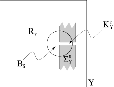
Figure 2: Sketch of the geometry around the end-point of the channel.

The subsequent proof is a sketch in so far as technical details in Step 2 are omitted.

Sketch of proof.

Step 1. Local $H^{1}$ estimate. We choose a cut-off function $\theta\in C_{c}^{\infty}(Y)$ which is identical to $1$ in $R_{Y}\cup\Sigma_{Y}^{\varepsilon}\cup K_{Y}^{\varepsilon}$ and use $\theta^{2}U_{\varepsilon}$ as a test function in equation (A.1) to obtain

$$\int_{Y\setminus\Sigma_{Y}^{\varepsilon}}|\nabla U_{\varepsilon}|^{2}\theta^{2}=-2\int_{Y\setminus\Sigma_{Y}^{\varepsilon}}\theta\nabla U_{\varepsilon}\cdot\nabla\theta\,U_{\varepsilon}+\omega^{2}\varepsilon^{2}\int_{Y\setminus\Sigma_{Y}^{\varepsilon}}|U_{\varepsilon}|^{2}\theta^{2}\,.$$

With Youngs inequality we conclude from the $L^{2}$-boundedness of $U_{\varepsilon}$ the $L^{2}$-boundedness of $\theta\nabla U_{\varepsilon}$.

Step 2. Estimates for $\partial_{1}U_{\varepsilon}$. We now want to obtain estimates for higher derivatives of the solution sequence. We recall that the lateral boundaries of the channel are straight and aligned with $e_{1}$. Furthermore, in a neighborhood of $\Gamma_{Y}^{\varepsilon,R}$, the boundary $\partial R_{Y}$ was assumed to be contained in a hypersurface with normal $e_{1}$.

We examine the solution in the ball $B_{\delta}:=B_{\delta}((y_{R},0))$, where $\delta>0$ is chosen so small that the boundary $\partial\Sigma_{Y}^{\varepsilon}\cap B_{\delta}$ consists of two pieces, a subset of the cylinder $\partial K_{Y}^{\varepsilon}$ and a subset of the plane $\{y_{R}\}\times\mathbb{R}^{n-1}$.

We study the function $V_{\varepsilon}:=\partial_{1}U_{\varepsilon}$ in $B_{\delta}$. The function $V_{\varepsilon}$ solves the Helmholtz $-\Delta V_{\varepsilon}=\omega^{2}\varepsilon^{2}V_{\varepsilon}$ (in the distributional sense) in $B_{\delta}\setminus\Sigma_{Y}^{\varepsilon}$. On the plane part of the boundary, $\partial\Sigma_{Y}^{\varepsilon}\cap\left(\{y_{R}\}\times\mathbb{R}^{n-1}\right)\cap B_{\delta}$, it satisfies the Dirichlet condition $V_{\varepsilon}=0$ (since $U_{\varepsilon}$ satisfies the homogeneous Neumann condition). On the cylindrical part of the boundary, $\partial K_{Y}^{\varepsilon}\cap\partial\Sigma_{Y}^{\varepsilon}\cap B_{\delta}$, it satisfies the homogeneous Neumann condition ($\partial_{\nu}V_{\varepsilon}=\partial_{1}\partial_{\nu}U_{\varepsilon}=0$).

The homogeneous boundary conditions allow to derive an estimate for $V_{\varepsilon}$: Multiplication of the Helmholtz equation for $V_{\varepsilon}$ with the solution $V_{\varepsilon}$ (multiplied with a cut-off function) provides local $H^{1}$-estimates for $V_{\varepsilon}$.

The above is not a rigorous proof: A priori, the function $V_{\varepsilon}$ is only of class $L^{2}$ (as a derivative of $U_{\varepsilon}$), hence testing the equation with $V_{\varepsilon}$ is not allowed. To obtain a rigorous proof, one has to proceed as follows: (a) Localize the problem and formulate boundary value problems for $U_{\varepsilon}$ and $V_{\varepsilon}$ in $B_{\delta}$ (or, better, for their truncated counterparts). (b) Show with the help of the Lax-Milgram lemma that the $V_{\varepsilon}$ problem posesses a solution $V_{\varepsilon}$ of class $H^{1}$. (c) Prove that the $y_{1}$-integrated solution solves the $U_{\varepsilon}$-problem and conclude from the uniqueness of the $U_{\varepsilon}$-problem that the $H^{1}$-function $V_{\varepsilon}$ coincides with $\partial_{1}U_{\varepsilon}$. We omit these technical details.

Step 3. Full high order estimate. In two space dimensions, we have obtained local $H^{2}$ estimates at this point: The second derivatives in the second direction can be expressed as $\partial_{2}^{2}U_{\varepsilon}=-\partial_{1}^{2}U_{\varepsilon}-\varepsilon^{2}\omega^{2}U_{\varepsilon}\in L^{2}$. We conclude that all second derivatives are bounded, $\|\Theta D^{2}U_{\varepsilon}\|_{L^{2}}\leq C$ for a cut-off function $\Theta$.

In space dimension $n=3$ we consider, for fixed $\zeta\in\mathbb{R}$, slices $S_{\zeta}:=\{y=(y_{1},y_{2},y_{3})|\,y_{1}=\zeta\}$. In every slice $S_{\zeta}$ the function $U_{\varepsilon}|_{S_{\zeta}}$ solves the two-dimensional problem $\Delta_{2}U_{\varepsilon}:=(\partial_{2}^{2}+\partial_{3}^{2})U_{\varepsilon}=-\partial_{1}^{2}U_{\varepsilon}-\varepsilon^{2}\omega^{2}U_{\varepsilon}\in L^{2}(S_{\zeta})$ for almost every $\zeta$. This provides estimates for all second spatial derivatives in $L^{2}$, locally around the interface.

Step 4. Sobolev embedding and conclusion. From the compact embedding $H^{2}(R_{Y})\subset C^{0}(R_{Y})$ we conclude that, up to a subsequence, the solution sequence $U_{\varepsilon}|_{R_{Y}}$ converges not only weakly in $H^{2}(R_{Y})$ to $\xi_{R}$, but also strongly in $C^{0}(R_{Y})$. This implies the first claim of (A.5). The second claim is shown by exactly the same calculation for $\Gamma_{Y}^{\varepsilon,Q}$. ∎

Acknowledgements

Support of both authors by DFG grant Schw 639/6-1 is greatfully acknowledged.

References

• [1] G. Allaire. Homogenization and two-scale convergence. SIAM J. Math. Anal., 23(6):1482–1518, 1992.
• [2] G. Allaire and M. Briane. Multiscale convergence and reiterated homogenisation. Proc. Roy. Soc. Edinburgh Sect. A, 126(2):297–342, 1996.
• [3] G. Allaire and C. Conca. Bloch wave homogenization and spectral asymptotic analysis. J. Math. Pures Appl. (9), 77(2):153–208, 1998.
• [4] M. Bellieud and G. Bouchitté. Homogenization of elliptic problems in a fiber reinforced structure. Nonlocal effects. Ann. Scuola Norm. Sup. Pisa Cl. Sci. (4), 26(3):407–436, 1998.
• [5] M. Bellieud and I. Gruais. Homogenization of an elastic material reinforced by very stiff or heavy fibers. Non-local effects. Memory effects. J. Math. Pures Appl. (9), 84(1):55–96, 2005.
• [6] G. Bouchitté and M. Bellieud. Homogenization of a soft elastic material reinforced by fibers. Asymptot. Anal., 32(2):153–183, 2002.
• [7] G. Bouchitté, C. Bourel, and D. Felbacq. Homogenization of the 3D Maxwell system near resonances and artificial magnetism. C. R. Math. Acad. Sci. Paris, 347(9-10):571–576, 2009.
• [8] G. Bouchitté and D. Felbacq. Low frequency scattering by a set of parallel metallic rods. In Mathematical and numerical aspects of wave propagation (Santiago de Compostela, 2000), pages 226–230. SIAM, Philadelphia, PA, 2000.
• [9] G. Bouchitté and D. Felbacq. Homogenization near resonances and artificial magnetism from dielectrics. C. R. Math. Acad. Sci. Paris, 339(5):377–382, 2004.
• [10] G. Bouchitté and D. Felbacq. Homogenization of a wire photonic crystal: the case of small volume fraction. SIAM J. Appl. Math., 66(6):2061–2084, 2006.
• [11] G. Bouchitté and B. Schweizer. Homogenization of Maxwell’s equations in a split ring geometry. Multiscale Model. Simul., 8(3):717–750, 2010.
• [12] G. Bouchitté and B. Schweizer. Plasmonic waves allow perfect transmission through sub-wavelength metallic gratings. Netw. Heterog. Media, 8(4):857–878, 2013.
• [13] Y. Chen and R. Lipton. Tunable double negative band structure from non-magnetic coated rods. New Journal of Physics, 12(8):083010, 2010.
• [14] K. D. Cherednichenko, V. P. Smyshlyaev, and V. V. Zhikov. Non-local homogenized limits for composite media with highly anisotropic periodic fibres. Proc. Roy. Soc. Edinburgh Sect. A, 136(1):87–114, 2006.
• [15] V. Chiadò Piat and M. Codegone. Scattering problems in a domain with small holes. RACSAM Rev. R. Acad. Cienc. Exactas Fís. Nat. Ser. A Mat., 97(3):447–454, 2003.
• [16] D. Cioranescu and F. Murat. A strange term coming from nowhere. In Topics in the mathematical modelling of composite materials, volume 31 of Progr. Nonlinear Differential Equations Appl., pages 45–93. Birkhäuser Boston, Boston, MA, 1997.
• [17] D. Cioranescu and J. Saint Jean Paulin. Homogenization in open sets with holes. J. Math. Anal. Appl., 71(2):590–607, 1979.
• [18] D. Cioranescu and J. Saint Jean Paulin. Homogenization of reticulated structures, volume 136 of Applied Mathematical Sciences. Springer-Verlag, New York, 1999.
• [19] C. Dörlemann, M. Heida, and B. Schweizer. Transmission conditions for the Helmholtz equation in perforated domains. Preprint 2015-02 of the TU Dortmund, 2015. http://hdl.handle.net/2003/34074.
• [20] S. Guenneau, F. Zolla, and A. Nicolet. Homogenization of 3D finite photonic crystals with heterogeneous permittivity and permeability. Waves Random Complex Media, 17(4):653–697, 2007.
• [21] V. V. Jikov, S. M. Kozlov, and O. A. Oleĭnik. Homogenization of differential operators and integral functionals. Springer-Verlag, Berlin, 1994. Translated from the Russian by G. A. Yosifian [G. A. Iosifyan].
• [22] R. Kohn and S. Shipman. Magnetism and homogenization of micro-resonators. Multiscale Modeling & Simulation, 7(1):62–92, 2007.
• [23] R. V. Kohn, J. Lu, B. Schweizer, and M. I. Weinstein. A variational perspective on cloaking by anomalous localized resonance. Comm. Math. Phys., 328(1):1–27, 2014.
• [24] A. Lamacz and B. Schweizer. Effective Maxwell equations in a geometry with flat rings of arbitrary shape. SIAM J. Math. Anal., 45(3):1460–1494, 2013.
• [25] A. Lamacz and B. Schweizer. A negative index meta-material for Maxwell´s equations. Preprint 2015-06 of the TU Dortmund, 2015. http://hdl.handle.net/2003/34176.
• [26] G. Nguetseng. A general convergence result for a functional related to the theory of homogenization. SIAM J. Math. Anal., 20(3):608–623, 1989.
• [27] S. O’Brien and J. Pendry. Magnetic activity at infrared frequencies in structured metallic photonic crystals. J. Phys. Condens. Mat., 14:6383 – 6394, 2002.
• [28] J. Pendry. Negative refraction makes a perfect lens. Phys. Rev. Lett., 85(3966), 2000.
• [29] E. Sánchez-Palencia. Nonhomogeneous media and vibration theory, volume 127 of Lecture Notes in Physics. Springer-Verlag, Berlin, 1980.
• [30] B. Schweizer. The low-frequency spectrum of small Helmholtz resonators. Proc. A., 471(2174):20140339, 18, 2015.
• [31] V. Veselago. The electrodynamics of substances with simultaneously negative values of $\varepsilon$ and $\mu$. Soviet Physics Uspekhi, 10:509–514, 1968.
• [32] V. V. Zhikov. Two-scale convergence and spectral problems of homogenization. Tr. Semin. im. I. G. Petrovskogo, (22):105–120, 333, 2002.