GeoReach: An Efficient Approach for Evaluating Graph Reachability Queries with Spatial Range Predicates

Abstract

Graphs are widely used to model data in many application domains. Thanks to the wide spread use of GPS-enabled devices, many applications assign a spatial attribute to graph vertices (e.g., geo-tagged social media). Users may issue a Reachability Query with Spatial Range Predicate (abbr. RangeReach). RangeReach finds whether an input vertex can reach any spatial vertex that lies within an input spatial range. An example of a RangeReach query is: Given a social graph, find whether Alice can reach any of the venues located within the geographical area of Arizona State University. The paper proposes GeoReach an approach that adds spatial data awareness to a graph database management system (GDBMS). GeoReach allows efficient execution of RangeReach queries, yet without compromising a lot on the overall system scalability (measured in terms of storage size and initialization/maintenance time). To achieve that, GeoReach is equipped with a light-weight data structure, namely SPA-Graph, that augments the underlying graph data with spatial indexing directories. When a RangeReach query is issued, the system employs a pruned-graph traversal approach. Experiments based on real system implementation inside Neo4j proves that GeoReach exhibits up to two orders of magnitude better query response time and up to four times less storage than the state-of-the-art spatial and reachability indexing approaches.

I Introduction

Graphs are widely used to model data in many application domains, including social networking, citation network analysis, studying biological function of genes, and brain simulation. A graph contains a set of vertices and a set of edges that connect these vertices. Each graph vertex or edge may possess a set of properties (aka. attributes). Thanks to the wide spread use of GPS-enabled devices, many applications assign a spatial attribute to a vertex (e.g., geo-tagged social media). Figure 1 depicts an example of a social graph that has two types of vertices: Person and Venue and two types of edges: Follow and Like. Vertices with type Person have two properties (i.e., attributes): name and age. Vertices with type Venue have two properties: name and spatial location. A spatial location attribute represents the spatial location of the entity (i.e., Venue) represented by such vertex. In Figure 1, vertices $\{e,f,g,h,i\}$ are spatial vertices which represent venues.

Figure 1: Location-Aware Social Graph

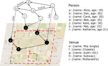
Graph Database Management Systems (GDBMSs) emerged as a prominent NoSQL approach to store, query, and analyze graph data [15, 8, 25, 24, 28]. Using a GDBMS, users can pose reachability analysis queries like: (i) Find out whether two vertices in the graph are reachable, e.g., Are Alice (vertex $a$) and Katharine (vertex $l$) reachable in the social graph given in Figure 1. (ii) Search for graph paths that match a given regular language expression representing predicates on graph elements, e.g., Find all venues that Alice’s Followees and/or her Followees’ Followees also liked. Similarly, users may issue a Reachability Query with Spatial Range Predicate (abbr. RangeReach). A RangeReach query takes as input a graph vertex $v$ and a spatial range $R$ and returns true only if $v$ can reach any spatial vertex (that possesses a spatial attribute) which lies within the extent of $R$ (formal definition is given in Section II). An example of a RangeReach query is: Find out whether Alice can reach any of the Venues located within the geographical area of Arizona State University (depicted as a dotted red rectangle $R$ in Figure 1). As given in Figure 1, The answer to this query is true since Alice can reach Sushi 101 (vertex $g$) which is located within $R$. Another query example is to find out whether Katharine can reach any of the venues located within $R$. The answer to this query is false due to the fact that the only venue reachable from Katharine, Subway (vertex $h$), is not located within $R$.

There are several straightforward approaches to execute a RangeReach query: (1) Traversal Approach: The naive approach traverses the graph, checks whether each visited vertex is a spatial vertex and returns true as the answer if the vertex’s spatial attribute lies within the input query range $R$. This approach yields no storage/maintenance overhead since no pre-computed data structure is maintained. However, the Traversal approach may lead to high query response time since the algorithm may traverse the whole graph to answer the query. (2) Transitive Closure (TC) Approach: this approach leverages the pre-computed transitive closure [27] of the graph to retrieve all vertices that are reachable from $v$ and returns true if at least one spatial vertex (located in the spatial range $R$) that is reachable from $v$. The TC approach achieves the lowest query response time, however it needs to pre-compute (and maintain) the graph transitive closure which is deemed notoriously infeasible especially for large-scale graphs. (3) Spatial-Reachability Indexing (SpaReach) Approach: uses a spatial index [3, 22] to locate all spatial vertices $V_{R}$ that lie within the spatial range $R$ and then uses a reachability index [35] to find out whether $v$ can reach any vertex in $V_{R}$. SpaReach achieves better query response time than the Traversal approach but it still needs to necessarily probe the reachability index for spatial vertices that may never be reached from the $v$. Moreover, SpaReach has to store and maintain two index structures which may preclude the system scalability.

In this paper, we propose GeoReach, a scalable and time-efficient approach that answers graph reachability queries with spatial range predicates (RangeReach). GeoReach is equipped with a light-weight data structure, namely SPA-Graph, that augments the underlying graph data with spatial indexing directories. When a RangeReach query is issued, the system employs a pruned-graph traversal approach. As opposed to the SpaReach approach, GeoReach leverages the Spa-Graph’ s auxiliary spatial indexing information to alternate between spatial filtering and graph traversal and early prunes those graph paths that are guaranteed: (a) not to reach any spatial vertex or (b) to only reach spatial vertices that outside the input spatial range query. As opposed to the TC and SpaReach approaches, GeoReach decides the amount of spatial indexing entries (attached to the graph) that strikes a balance between query processing efficiency on one hand and scalability (in terms of storage overhead) on the other hand. In summary, the main contributions of this paper are as follows:

• To the best of the authors’ knowledge, the paper is the first that formally motivates and defines RangeReach, a novel graph query that enriches classic graph reachability analysis queries with spatial range predicates. RangeReach finds out whether an input graph vertex can reach any spatial vertex that lies within an input spatial range.

• The paper proposes GeoReach a generic approach that adds spatial data awareness to an existing GDBMS. GeoReach allows efficient execution of RangeReach queries issued on a GDBMS, yet without compromising a lot on the overall system scalability (measured in terms of storage size and initialization/maintenance time).

• The paper experimentally evaluates GeoReach  using real graph datasets based on a system implementation inside Neo4j (an open source graph database system). The experiments show that GeoReach exhibits up to two orders of magnitude better query response time and occupies up to four times less storage than the state-of-the-art spatial and reachability indexing approaches.

The rest of the paper is organized as follows: Section II lays out the preliminary background and related work. The SPA-Graph data structure, GeoReach query processing, initialization and maintenance algorithms are explained in Sections III to V. Section VI experimentally evaluates the performance of GeoReach. Finally, Section VII concludes the paper.

II Preliminaries and Background

This section highlights the necessary background and related research work. Table I summarizes the main notations in the paper.

II-A Preliminaries

Notation	Description
$G=\{V,E\}$	A graph $G$ with a set of vertices $V$ and set of edges $E$
$V_{v}^{out}$	The set of vertices that can be reached via a direct edge from a vertex $v$
$V_{v}^{in}$	The set of vertices that can reach (via a direct edge) vertex $v$
$RF(v)$	The set of vertices that are reachable from (via any number of edges) vertex $v$
$V_{S}$	The set of spatial vertices in $G$ such that $V_{S}\subseteq V$
$RF_{S}(v)$	The set of spatial vertices that are reachable from (via any number of edges) vertex $v$
$n$	The cardinality of V ($n=|V|$); the number of vertices in $G$
$m$	The cardinality of E ($m=|E|$); the number of edges in $G$
$v_{1}\leadsto v_{2}$	$v_{2}$ is reachable from $v_{1}$ via connected path in $G$ (such that both $v_{1}$ and $v_{2}$ $\in$ $V$)
MBR($P$)	Minimum bounding rectangle of a set of spatial polygons $P$ (e.g., points, rectangles)

TABLE I: Notations.

Graph Data. GeoReach deals with a directed property graph $G=(V,E)$ where (1) $V$ is a set of vertices such that each vertex has a set of properties (attributes) and (2) $E$ is a set of edges in which every edge can be represented as a tuple of two vertices $v_{1}$ and $v_{2}$ ($v_{1},v_{2}\in V$). The set of spatial vertices $V_{S}\subseteq V$ such that each $v\in V_{S}$ has a spatial attribute (property) $v.spatial$. The spatial attribute $v.spatial$ may be a geometrical point, rectangle, or a polygon. For ease of presentation, we assume that a spatial attribute of spatial vertex is represented by a point. Figure 1 depicts an example of a directed property graph. Spatial Vertices $V_{S}$ are represented by black colored circles and are located in a two-dimensional planer space while white colored circles represent regular vertices that do not possess a spatial attribute. Arrows indicate directions of edges in the graph.

Graph Reachability ($v_{1}\leadsto v_{2}$). Given two vertices $v_{1}$ and $v_{2}$ in a graph $G$, $v_{1}$ can reach $v_{2}$ ($v_{1}\leadsto v_{2}$) or in other words $v_{2}$ is reachable from $v_{1}$ if and only if there is at least one graph path from $v_{1}$ to $v_{2}$. For example, in Figure 1, vertex $a$ can reach vertex $f$ through the graph path a->c->i->f so it can be represented as $a\leadsto f$. On the other hand, $c$ cannot reach $h$.

Reachability with Spatial Range Predicate (RangeReach). RangeReach queries find whether a graph vertex can reach a specific spatial region (range) $R$. Given a vertex $v\in V$ in a Graph $G$ and a spatial range $R$, RangeReach can be described as follows:

$$\emph{\small RangeReach(v, R)}=\left\{\,\begin{IEEEeqnarraybox}[]{[}][c]{l?s}\IEEEstrut{true}&if$\exists$~{}$v'$suchthat\\ {}&~{}(1)~{}$v' \in V_{S}$\\ {}&~{}(2)~{}$v'.spatial$lieswithin$R$\\ {}&~{}(3)~{}$v \leadsto v'$\\ {false}&Otherwise.\IEEEstrut\end{IEEEeqnarraybox}\right.$$ (1)

As given in Equation 1, if any spatial vertex $v^{\prime}\in V_{S}$ that lies within the extent of the spatial range $R$ is reachable from the input vertex $v$, then RangeReach($v$, $R$) returns true (i.e., $v\leadsto R$). For example, in Figure 1, RangeReach($a$, $R$) = true since $a$ can reach at least one spatial vertex $f$ in $R$. However, RangeReach($l$, $R$) = false since $l$ can merely reach a spatial vertex $h$ which is not located in $R$. Vertex $d$ cannot reach $R$ since it cannot reach any vertex.

II-B Related Work

This section presents previous work on reachability indexes, spatial indexes, and straightforward solutions to processing graph reachability queries with spatial range predicates (RangeReach).

Reachability Index. Existing solutions to processing graph reachability queries ($u\leadsto v$) can be divided into three categories [35]: (1) Pruned Graph Traversal [6, 30, 34]: These approaches pre-compute some auxiliary reachability information offline. When a query is issued, the query processing algorithm traverses the graph using a classic traversal algorithm, e.g., Depth First Search (DFS) or Breadth First Search (BFS), and leverages the pre-computed reachability information to prune the search space. (2) Transitive closure retrieval [1, 7, 17, 18, 27, 31, 32]: this approach pre-computes the transitive closure of a graph offline and compresses it to reduce its storage footprint. When a query $u\leadsto v$ is posed, the transitive closure of the source vertex $u$ is fetched and decomposed. Then the query processing algorithm checks whether the terminal vertex $v$ lies in the transitive closure of $u$. and (3) Two-Hop label matching [5, 8, 10, 11, 12, 26]: The two-hop label matching approach assigns each vertex $v$ in the graph an out-label set $L_{out}(v)$ and an in-label set $L_{in}(v)$. When a reachability query is answered, the algorithm decides that $u\leadsto v$ if and only if $L_{out}(v)\cap L_{in}(v)\not\neq\varnothing$. Since the two label sets do not contain all in and out vertices, size of the reachability index reduces.

Spatial Index. A spatial index  [21, 23, 29] is used for efficient retrieval of either multi-dimensional objects (e.g., $\langle$$x$,$y$$\rangle$ coordinates of an object location) or objects with spatial extents, e.g., polygon areas represented by their minimum boundary rectangles (MBR). Spatial index structures can be broadly classified to hierarchical (i.e., tree-based) and non-hierarchical index structures. Hierarchical tree-based spatial index structures can be classified into another two broad categories: (a) the class of data-partitioning trees, also known as the class of Grow-and-Post trees [20], which refers to the class of hierarchical data structures that basically extend the B-tree index structure [2, 13] to support multi-dimensional and spatial objects. The main idea is to recursively partition the spatial data based on a spatial proximity clustering, which means that the spatial clusters may overlap. Examples of spatial index structures in this category include R-tree [16] and R*-tree [3]. (b) the class of space-partitioning trees that refers to the class of hierarchical data structures that recursively decomposes the space into disjoint partitions. Examples of spatial index structures in this category include the Quad-tree [14] and k-d tree [4].

Spatial Data in Graphs. Some existing graph database systems, e.g., Neo4j, allow users to define spatial properties on graph elements. However, these systems do not provide native support for RangeReach queries. Hence, users need to create both a spatial index and a reachability index to efficiently answer a RangeReach queries (drawbacks of this approach are given in the following section). On the other hand, existing research work [19] extends the RDF data with spatial data to support RDF queries with spatial predicates (including range and spatial join). However, such technique is limited to RDF and not general graph databases. It also does not provide an efficient solution to handle reachability queries.

II-C Straightforward Solutions

There are three main straightforward approaches to process a RangeReach query, described as follows:

Approach I: Graph Traversal. This approach executes a spatial reachability query using a classical graph traversal algorithm like DFS (Depth First Search) or BFS (Breadth First Search). When RangeReach($v$, $R$) is invoked, the system traverses the graph from the starting vertex $v$. For each visited vertex, the algorithm checks whether it is a spatial vertex and returns true as the query answer if the vertex’s location lies within the input query range $R$ because the requirement of spatial reachability is satisfied and hence $v\leadsto R$. Otherwise, the algorithm keeps traversing the graph. If all vertices that $v$ can reach do not lie in $R$, that means $v$ cannot reach $R$.

Approach II: Transitive Closure (TC). This approach pre-computes the transitive closure of the graph and stores it as an adjacency matrix in the database. Transitive closure of a graph stores the connectivity component of the graph which can be used to answer reachability query in constant time. Since the final result will be determined by spatial vertices, only spatial vertices are stored. When RangeReach($v$, $R$) is invoked, the system retrieves all spatial vertices that are reachable from $v$ by means of the transitive closure. The system then returns true if at least one spatial vertex that is reachable from $v$ is also located in the spatial range $R$.

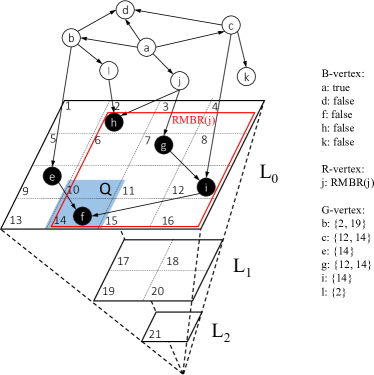
Approach III: SpaReach. This approach constructs two indexes a-priori: (1) A Spatial Index: that indexes all spatial vertices in the graph and (2) A Reachability Index: that indexes the reachability information of all vertices in the graph. When a RangeReach query is issued, the system first takes advantage of the spatial index to locate all spatial vertices $V_{R}$ that lie within the spatial range $R$. For each vertex $v^{\prime}\in V_{R}$, a reachability query against the reachability index is issued to test whether $v$ can reach $v^{\prime}$. For example, to answer RangeReach($a$, $R$) in Figure 2, spatial index is exploited first to retrieve all spatial vertices that are located in $R$. From the range query result, it can be known that $g$, $i$ and $f$ are located in rectangle $R$. Then graph reachability index is accessed to determine whether $a$ can reach any located-in vertex. Hence, it is obvious RangeReach($a$, $R$) = true by using this approach.

Critique. The Graph Traversal approach yields no storage/maintenance overhead since no pre-computed data structure is maintained. However, the traversal approach may lead to high query response time ($O(m)$ where $m$ is the number of edges in the graph) since the algorithm may traverse the whole graph to answer the query. The TC approach needs to pre-compute (and maintain) the graph transitive closure which is deemed notoriously infeasible especially for large-scale graphs. The transitive closure computation is $O(kn^{3})$ or $O(nm)$ and the TC storage overhead is $O(kn^{2})$ where $n$ is total number of vertices and $k$ is the ratio of spatial vertices to the total number of vertices in the graph. To answer a RangeReach query, the TC approach takes $O(kn)$ time since it checks whether each reachable spatial vertex in the transitive closure is located within the query rectangle. On the other hand, SpaReach builds a reachability index, which is a time-consuming step, in $O(n^{3})$ [32] time. The storage overhead of a spatial index is $O(n)$ and that of a reachability index is $O(nm^{1/2})$. To store the two indices, the overall storage overhead is $O(nm^{1/2})$. Storage cost of this approach is far less than TC approach but still not small enough to accommodate large-scale graphs. The query time complexity of a spatial index is $O(kn)$ while that of reachability index is $m^{1/2}$. But for a graph reachability query, checking is demanded for each spatial vertex in the result set generated by the range query. Hence, cost of second step reachability query is $O(knm^{1/2})$. The total cost should be $O(knm^{1/2})$. Query performance of Spa-Reach is highly impacted by the size of the query rectangle since the query rectangle determines how many spatial vertices are located in the region. In Figure 1, query rectangle $R$ overlaps with three spatial vertices. For example, to answer RangeReach($l$, $R$), all three vertices $\{f,g,i\}$ will be checked against the reachability index to decide whether any of them is reachable from $l$ and in fact neither of them is reachable. In a large graph, a query rectangle will possibly contain a large number of vertices. That will definitely lead to high unreasonable high query response time.

Figure 2: SPA-Graph Overview

III Our Approach: GeoReach

In this section, we give an overview of GeoReach an efficient and scalable approach for executing graph reachability queries with spatial range predicates.

III-A Data Structure

In this section, we explain how GeoReach augments a graph structure with spatial indexing entries to form what we call SPatially-Augmented Graph (SPA-Graph). To be generic, GeoReachstores the newly added spatial indexing entries the same way other properties are stored in a graph database system. The structure of a SPA-Graph is similar to that of the original graph except that each vertex $v\in V$ in a SPA-Graph $G=\{V,E\}$ stores spatial reachability information. A SPA-Graph has three different types of vertices, described as follows:

• B-Vertex: a B-Vertex $v$ ($v\in V$) stores an extra bit (i.e., boolean), called Spatial Reachability Bit (abbr. GeoB) that determines whether $v$ can reach any spatial vertex ($u\in V_{S}$) in the graph. GeoB of a vertex $v$ is set to 1 (i.e., true) in case $v$ can reach at least one spatial vertex in the graph and reset to 0 (i.e., false) otherwise.

• R-Vertex: an R-Vertex $v$ ($v\in V$) stores an additional attribute, namely Reachability Minimum Bounding Rectangle (abbr. RMBR($v$)). RMBR($v$) represents the minimum bounding rectangle MBR($S$) (represented by a top-left and a lower-right corner point) that encloses all spatial polygons which represent all spatial vertices $S$ that are reachable from vertex $v$ (RMBR($v$) = MBR($RF_{S}(v)$), $RF_{S}(v)$ = $\{u|v\leadsto u,u\in V_{S}\}$).

• G-Vertex: a G-Vertex $v$ stores a list of spatial grid cells, called the reachability grid list (abbr. ReachGrid($v$)). Each grid cell $C$ in ReachGrid($v$) belongs to a hierarchical grid data structure that splits the total physical space into $n$ spatial grid cells. Each spatial vertex $u\in V_{S}$ will be assigned a unique cell ID $(k\in[1,n])$ in case $u$ is located within the extents of cell $k$, noted as Grid$(u)=k$. Each cell $C\in$ ReachGrid($v$) contains at least one spatial vertex that is reachable from $v$ (ReachGrid($v$) = $\cup~{}$Grid($u$), $\{u|v\leadsto u,~{}{u\in{V_{S}}}\}$).

Lemma III.1

Let $v$ ($v\in V$) be a vertex in a SPA-Graph $G=\{V,E\}$ and $V_{v}^{out}$ be the set of vertices that can be reached via a direct edge from a vertex $v$. The reachability minimum bounding rectangle of $v$ (RMBR($v$)) is equivalent to the minimum bounding rectangle that encloses all its out-edge neighbors $V_{v}^{out}$ and their reachability minimum bounding rectangles. RMBR($v$) = MBR${}_{v^{\prime}\in V_{v}^{out}}$(RMBR($v^{\prime}$), $v^{\prime}.spatial$).

Proof:

Based on the reachability definition, the set of reachable vertices $RF(v)$ from a vertex $v$ is equal to the union of the set of vertices that is reached from $v$ via a direct edge ($V_{v}^{out}$) and all vertices that are reached from each vertex $v^{{}^{\prime}}\in V_{v}^{out}$. Hence, the set ($RF_{S}(v)$) of reachable spatial vertices from $v$ is given in Equation 2.

$$RF_{S}(v)=\bigcup\limits_{v^{{}^{\prime}}\in V_{v}^{out}}(v^{\prime}\cup RF_{S}(v^{{}^{\prime}}))$$ (2)

And since RMBR($v$) = MBR($RF_{S}(v)$), then the the reachability minimum bounding rectangle of $v$ is as follows:

$$\begin{split}{RMBR}(v)&={MBR}(\bigcup\limits_{v^{{}^{\prime}}\in V_{v}^{out}}(v^{\prime}\cup RF_{S}(v^{{}^{\prime}}))))\\ &={MBR}_{v^{\prime}\in V_{v}^{out}}(RMBR(v^{\prime}),v^{\prime}.spatial)\end{split}$$ (3)

That concludes the proof. ∎

Lemma III.2

The set of reachable spatial grid cells from a given vertex $v$ is equal to the union of all spatial grid cells reached from its all its out-edge neighbors and grid cells that contain the spatial neighbors

$$ReachGrid(v)=\bigcup\limits_{v^{\prime}\in V_{v}^{out}}(ReachGrid(v^{\prime})\cup Grid(v^{\prime}))$$ (4)

Proof:

Similar to that of Lemma III.1. ∎

Example. Figure 2 gives an example of a SPA-Graph. GeoB of vertex $b$ is set to $1$ (true) since $b$ can reach three spatial vertices $e$, $f$ and $h$. GeoB for $d$ is $0$ since $d$ cannot reach any spatial vertex in the graph. Figure 2 also gives an example of a Reachability Minimum Bounding Rectangle RMBR of vertex $j$ (i.e., RMBR($j$)). All reachable spatial vertices from $j$ are $g$, $i$, $h$ and $f$. Figure 2 also depicts an example of ReachGrid. There are three layers of grids, denoted as $L_{0}$, $L_{1}$, $L_{2}$ from top to bottom. The uppermost layer $L_{0}$ is split into $4\times 4$ grid cells; each cell is assigned a unique id from $1$ to $16$. We denote grid cell with id $1$ as $G_{1}$ for brevity. The middle layer gird $L_{1}$ is split into four cells $G_{17}$ to $G_{20}$. Each cell in $L_{1}$ covers four times larger space than each cell in $L_{0}$. $G_{17}$ in $L_{1}$ covers exactly the same area of $G_{1}$, $G_{2}$, $G_{5}$, $G_{6}$ in $L_{0}$. The bottom layer $L_{2}$ contains only a single grid cell which covers all four grids in $L_{1}$ and represents the whole physical space. All spatial vertices reachable from vertex $a$ are located in $G_{2}$, $G_{7}$, $G_{9}$, $G_{12}$ and $G_{14}$, respectively. Hence, ReachGrid($a$) can be $\{2,7,9,12,14\}$. Notice that vertex $e$ and $f$ are both located in $G_{9}$ and $G_{14}$ covered by $G_{19}$ in ReachGrid($a$) can be replaced by $G_{19}$. Then, ReachGrid($a$) = $\{2,7,12,19\}$. In fact, there exist more options to represent ReachGrid($a$), such as $\{17,18,19,20\}$ or $\{21\}$ by merging into only a single grid cell in $L_{2}$. When we look into ReachGrid of connected vertices, for instance $g$, ReachGrid($g$) is $\{12,14\}$ and ReachGrid($i$) is $\{14\}$. It is easy to verify that ReachGrid($g$) is ReachGrid($i$)$\cup$Grid($i.spatial$), which accords with lemma III.2.

SPA-Graph Intuition. The main idea behind the SPA-Graph is to leverage the spatial reachability bit, reachability minimum bounding rectangle and reachability grid list stored in a B-Vertex, R-Vertex or a G-Vertex to prune graph paths that are guaranteed (or not) to satisfy both the spatial range predicate and the reachability condition. That way, GeoReach cuts down the number of traversed graph vertices and edges and hence significantly reduce the overall latency of a RangeReach query.

III-B Query Processing

Algorithm 1 Reachability Query with Spatial Range Predicate

1: Function RangeReach($v$, $R$)

2: if v is a spatial vertex and $v.spatial$ Lie In $R$ then return true

3: Terminate $\leftarrow$ true

4: if $v$ is a B-vertex then

5:    if GeoB($v$) = true then Terminate $\leftarrow$ false

6: else if $v$ is a R-vertex then

7:    if $R$ full contains RMBR($v$) then return true

8:    if $R$ no overlap with RMBR($v$) then return false

9:    Terminate $\leftarrow$ false

10: else if $v$ is a G-vertex then

11:    for each grid $G_{i}\in$ ReachGrid($v$) do

12:       if $R$ fully contains $G_{i}$ then return true

13:       $G_{i}$ partially overlaps with $R$ then Terminate $\leftarrow$ false

14: if Terminate = false then

15:    for each vertex $v^{\prime}\in V_{v}^{out}$ do

16:       if RangeReach($v^{\prime}$, $R$) = true then return true

17: return false

This section explains the RangeReach query processing algorithm. The main objective is to visit as less graph vertices and edges as possible to reduce the overall query latency. The query processing algorithm accelerates the SPA-Graph traversal procedure by pruning those graph paths that are guaranteed (or not) to satisfy the spatial reachability constraint. Algorithm 1 gives pseudocode for query processing. The algorithm takes as input a graph vertex $v$ and query rectangle $R$. It then starts traversing the graph starting from $v$. For each visited vertex $v$, three cases might happen, explained as follows:

Case I (B-vertex): In case GeoB is false, a B-vertex cannot reach any spatial vertex and hence the algorithm stops traversing all graph paths after this vertex. Otherwise, further traversal from current B-vertex is required when GeoB value is true. Line 4 to 5 in algorithm 1 is for processing such case.

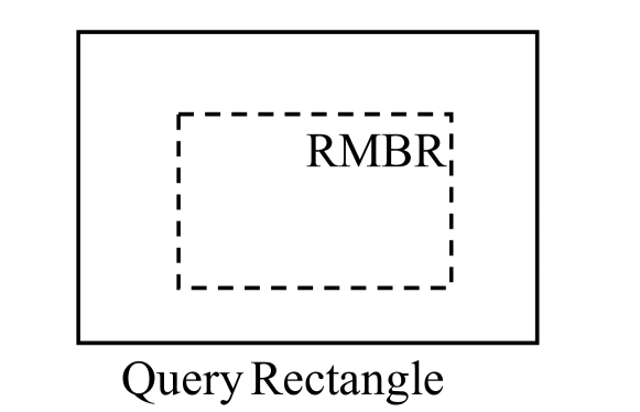
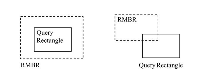
Case II (R-vertex): For a visited R-vertex $u$, there are three conditions that may happen (see figure 3). They are the case from line 6 to 9 in algorithm 1:

• Case II.A: RMBR($u$) lies within the query rectangle (see Figure 3(b)). In such case, the algorithm terminates and returns true as the answer to the query since there must exist at least a spatial vertex that is reachable from $v$.

• Case II.B: The spatial query region $R$ does not overlap with RMBR($u$) (see Figure 3(a)). Since all reachable spatial vertices of $u$ must lie inside RMBR($u$), there is no reachable vertex can be located in the query rectangle. As a result, graph paths originating at $u$ can be pruned.

• Case III.C: RMBR($u$) is partially covered by the query rectangle (see Figure 3(c)). In this case, the algorithm keeps traversing the graph by fetching the set of vertices $V_{v}^{out}$ that can be reached via a direct edge from $v$.

(a) No Overlap

(b) Lie In

(c) Partially Covered By

Figure 3: Relationships between RMBR and a query rectangle

Case III (G-vertex): For a G-vertex $u$, it store many reachable grids from $u$. Actually, it can be regarded as many smaller RMBRs. So three cases may also happen. Algorithm 1 line 13 to 18 is for such case. Three cases will happen are explained as follows:

• Case III.A: The query rectangle $R$ fully contains any grid cell in ReachGrid($u$). In such case, the algorithms terminates and returns true as the query answer.

• Case III.B: The query rectangle have no overlap with all grids in ReachGrid($u$). This case means that $v$ cannot reach any grids overlapped with $R$. Then we never traverse from $v$ and this search branch is pruned.

• Case III.C: If the query rectangle fully contains none of the reachable grid and partially overlap with any reachable grid, it corresponds to Partially Covered By case for RMBR. So further traversal is performed.

Figure 2 gives an example of RangeReach that finds whether vertex $a$ can reach query rectangle $Q$ (the shaded one in figure 2). At the beginning of the traversal, the algorithm checks the category of $a$. In case, It is a B-vertex and its GeoB value is true, the algorithm recursively traverses out-edge neighbors of $a$ and perform recursive checking. Therefore, the algorithm retrieves vertices $b$, $c$, $d$ and $j$. For vertex $b$, it is a G-vertex and its reachable grids are $G_{2}$ and $G_{19}$. $G_{19}$ cover the range of four grids in $L_{0}$. They are $G_{9}$, $G_{10}$, $G_{13}$ and $G_{14}$. The spatial range is merely partially covered by $Q$ (Case III.C), hence it is possible for $b$ to reach $Q$. We cannot make an assured decision in this step so $b$ is recorded for future traversal. Another neighbor is $c$. ReachGrid($c$) is $\{12,14\}$ which means that $G_{12}$ and $G_{14}$ are reachable from $c$. $G_{14}$ lies in $Q$ (Case III.A). In such case, since $a\leadsto c$, we can conclude that $a\leadsto R$. The algorithm then halts the graph traversal at this step and returns true as the query answer.

IV SPA-Graph Analysis

This section analyzes each SPA-Graph vertex type rom two perspectives: (1) Storage Overhead: the amount of storage overhead that each vertex type adds to the system (2) Pruning Power: the probability that the query processing algorithm terminates when a vertex of such type is visited during the graph traversal.

B-vertex. When visiting a B-Vertex, in case GeoB is false, the query processing algorithm prunes all subsequent graph paths originated at such vertex. That is due to the fact that such vertex cannot reach any spatial vertex in the graph. Otherwise, the query processing algorithm continues traversing the graph. As a result, pruned power of a B-vertex lies in the condition that GeoB is false. For a given graph, number of vertices that can reach any space is a certain value. So probability that a vertex can reach any spatial vertex is denoted as $P_{true}$. This is also the probability of a B-vertex whose GeoB value is true. Probability of a B-vertex whose GeoB value is false, denoted as $P_{false}$, will be $1-P_{true}$. To sum up, pruned power of a B-vertex is $1-P_{true}$ or $P_{false}$

(a)

(b)

(c)

Figure 4: R-vertex Pruning Power

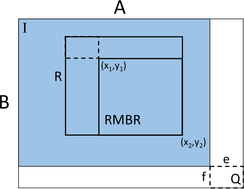
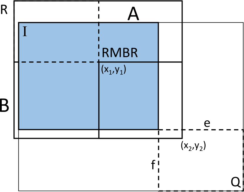
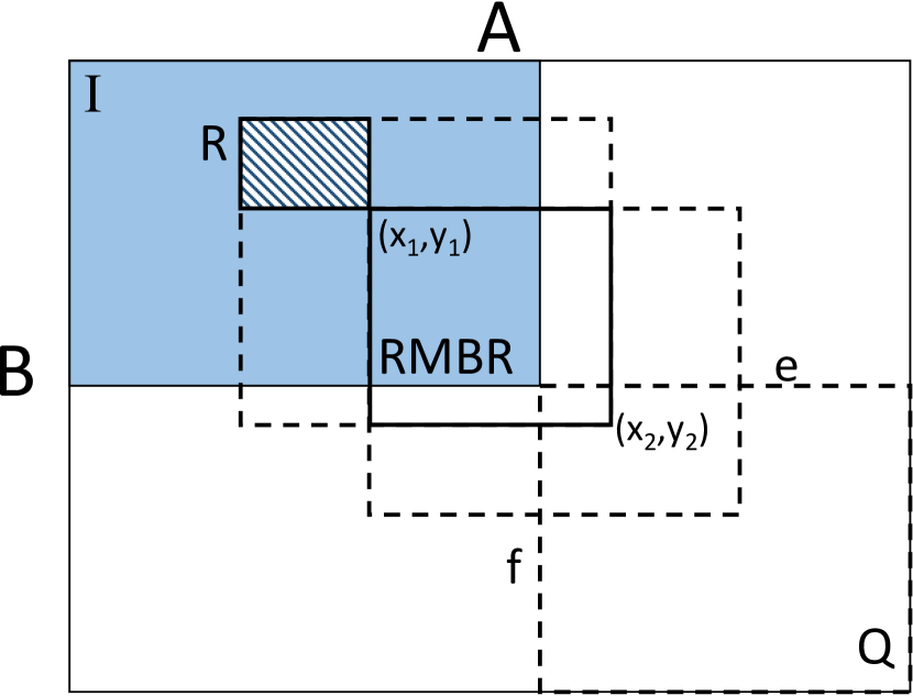
R-vertex. When an R-vertex is visited, the condition whether the vertex can reach any space still exists. If the R-vertex cannot reach any space, we assign the R-vertex a specific value to represent it(e.g. set coordinates of RMBR’s bottom-left point bigger than that of the top-right point). In this case, pruned power of a R-vertex will be the same with a B-vertex, which is $P_{false}$. Otherwise, when the R-vertex can reach some space, it will be more complex. Because information of RMBR and query rectangle $R$ have some impact on the pruned power of this R-vertex. The algorithm stops traversing the graph in both the No Overlap and Lie In cases depicted in Figures 3(a) and 3(b). Figure 4 shows the two cases that R-vertex will stop the traversal. In Figure 4, width and height of the total 2D space are denoted as $A$ and $B$. Assume that the query rectangle can be located anywhere in the space with equal probability. We use $(x_{1},y_{1})$ and $(x_{2},y_{2})$ to represent the RMBR’s top-left corner and lower-right point coordinates, respectively. Then all possible areas where top-left vertex of query rectangle $Q$ should be part of the total space, denoted as $I$ (see the shadowed area in the figure. Its area is determined by size of query rectangle. Denote width and height of $Q$ are $e$ and $f$, then area of $I$, $A_{I}=(A-e)\times(B-f)$.

First, we estimate probability of No Overlap case. Figure 4(a) shows one case of No Overlap. If the query rectangle $Q$ do not overlap with RMBR, top-left vertex of $Q$ must lie outside rectangle $R$ which is forms the overlap region (drawn with solid line in Figure 4(b)). Area of $R$ (denoted as $A_{R}$) is obviously determined by the RMBR location and size of $Q$. It can be easily observed that $A_{R}=(x_{2}-(x_{1}-e))\times(y_{2}-(y_{1}-f))$. Another possible case is demonstrated in Figure 4(b). In such case, if we calculate $R$ in the same way, range of $R$ will exceeds area of $I$ which contains all possible locations. As a result, $A_{R}=A_{I}$ in this case. As we can see, area of overlap region is determined by the range of $R$ and $I$ altogether. Then we can have a general representation of the overlap area $A_{Overlap}=(min(A-e,x_{2})-max(0,x_{1}-e))\times(min(B-f,y_{2})-max(0,x_{2}-f)$. The No Overlap area is $A_{I}-A_{Overlap}$ and the probability of having a No Overlap case is calculated as follows:

$$P_{NoOverlap}=\frac{A_{I}-A_{Overlap}}{A_{I}}=1-\frac{A_{Overlap}}{A_{I}}.$$ (5)

Figure 4(c) depicts the Lie In case. When top-left vertex of $Q$ lies in region $R$, then such Lie In case will happen. To ensure that $R$ exists, it is necessary that $e>(x_{2}-x_{1})$ and $f>(y_{2}-y_{1})$. If it is not, then probability of such case must be 0. If this requirement is satisfied, then $A_{R}=(x_{1}-(x_{2}-e))\times(y_{1}-(y_{2}-f))$. Recall what is met in the above-mentioned case, $R$ may exceed the area of $I$. Similarly, more general area should be $A_{R}=(min(A-e,x_{1})-max(0,x_{1}-(x_{2}-e)))\times(min(B-f,y_{1})-max(0,y_{1}-(y_{2}-f)))$. Probability of such case should be $\frac{A_{R}}{A_{I}}$. To sum up, we have

$$P_{LieIn}=\begin{cases}\frac{A_{R}}{A_{I}}&\mbox{$e>(x_{2}-x_{1})$ and $f>(y_{2}-y_{1})$}\\ 0&\mbox{else}\end{cases}$$ (6)

After we sum up all conditional probabilities based on $P_{true}$ and $P_{false}$, pruning power of an R-vertex is equal to $(P_{\small NoOverlap}+P_{\small LieIn})\times P_{true}+P_{false}$. Evidently, the pruning power of an R-vertex is more powerful than a B-vertex. When the storage overhead of an R-vertex is considered, coordinates of RMBR’s top-left and lower-right vertices should be stored. Thus its storage will be at least four bytes depending on the spatial data precision. That means the storage overhead of a G-Vertex is always higher than that of a B-Vertex.

G-vertex. For a high resolution grid, it is of no doubt that a G-vertex possesses a high pruning power. However, this comes at the cost of higher storage overhead because more grid cells occupies more space. When a G-vertex is compared with an R-vertex, the area of an R-vertex is much larger than a grid. In this case, an R-vertex can be seen as a a simplified G-vertex for which the grid cell size is equal to that of RMBR. One extreme case of R-vertex is that the vertex can reach only one spatial vertex. In such case, RMBR is location of the reachable spatial vertex. Such R-vertex can still be counted as a G-vertex whose grid size $x\rightarrow 0$. According the rule, it should be with higher storage overhead and more accuracy. Actually, storing it as a G-vertex will cost an integer while any R-vertex requires storage for four float or even double number.

V Initialization & Maintenance

Algorithm 2 GeoReach Initialization Algorithm

1: Function Initialize(Graph $G=\{V,E\}$)

2: /*PHASE I: SPA-Graph Vertex Initialization */

3: for each Vertex $v$ $\in$ $V$ according their sequence in topology do

4:    InitializeVertex($G$, $v$, MAX_REACH_GRIDS, MAX_RMBR)

5: /* PHASE II: Reachable Grid Cells Merging */

6: for each G-vertex $v$ do

7:    for each layer $L_{i}$ from $L_{1}$ to $L_{bottom}$ do

8:       for each grid cell $G_{i}$ in $L_{i}$ do

9:          if Number of reachable grids in corresponding region in $L_{i-1}$ is larger than MERGE_COUNT then

10:             Add $G_{i}$ in $L_{i}$ into ReachGrid($v$)

11:             Remove reachable grid cells that are covered by $G_{i}$ in higher layers

This section describes the SPA-Graph initialization algorithm. The GeoReach initialization algorithm (Pseudocode is given in Algorithm 2) takes as input a graph Graph $G=\{V,E\}$ and runs in two main phases: (1) Phase I: SPA-Graph Vertex Type Initialization: this phase leverages the tradeoff between query response time and storage overhead explained in Section IV to determine the type of each vertex. (2) Phase II: Reachable Grid Cells Merging: This step further reduces the storage overhead of each G-Vertex in the SPA-Graph by merging a set of grid cells into a single grid cell. Details of each phase are described in Section V-A and V-B

V-A SPA-Graph Vertex Type Initialization

Algorithm 3 SPA-Graph Vertex Initialization Algorithm

1: Function InitializeVertex(Graph $G=\{V,E\}$, Vertex $v$)

2: Type $\leftarrow$ InitializeType(v)

3: switch (Type)

4: case B-vertex:

5:    Set $v$ B-vertex and GeoB($v$) = true

6: case G-vertex:

7:    ReachGrid($v$) $\leftarrow$ $\emptyset$

8:    for each Vertex $v{{}^{\prime}}$ $\in$ $V_{v}^{out}$ do

9:       Maintain-GVertex($v$, $v^{\prime}$)

10:       if Number of grids in ReachGrid($v$) ¿ MAX_REACH_GRIDS then

11:          Set $v$ R-vertex and break

12:    Type $\leftarrow$ R-vertex

13:    if Number of grids in ReachGrid($v$) = 0 then

14:       Set $v$ B-vertex, GeoB($v$) $\leftarrow$ false and break

15: case R-vertex:

16:    RMBR($v$) $\leftarrow$ $\emptyset$

17:    for each Vertex $v{{}^{\prime}}$ $\in$ $V_{v}^{out}$ do

18:       Maintain-RVertex($v$, $v^{\prime}$)

19:       if Area(RMBR($v$)) ¿ MAX_RMBR then

20:          Set $v$ B-vertex, GeoB($v$) $\leftarrow$ true and break

21: end switch

To determine the type of each vertex, the initialization algorithm takes into account the following system parameters:

• MAX_RMBR: This parameter represents a threshold that limits space area of each RMBR. If a vertex $v$ is an R-vertex, area of RMBR($v$) cannot be larger than MAX_RMBR. Otherwise, $v$ will be degraded to a B-vertex.

• MAX_REACH_GRIDS: This parameter sets up the maximum number of grid cells in each ReachGrid. If a vertex $v$ is a G-vertex, number of grid cells in ReachGrid($v$) cannot exceed MAX_REACH_GRIDS. Otherwise, $v$ will be degraded to an R-vertex.

Algorithm 3 gives the pseudocode of the vertex initialization algorithm. Vertices are processed based on their topological sequence in the graph. For each vertex, the algorithm first determines the initial vertex type using the InitializeType function (pseudocode omitted for brevity). For a vertex $v$, categories of vertex $v^{\prime}$ ($\{v^{\prime}|~{}v^{\prime}\in V_{v}^{out}\}$) will be checked. If there is any B-vertex $v^{\prime}$ with GeoB($v^{\prime}$) = true, $v$ is directly initialized to a B-vertex with GeoB($v$) = true. Otherwise, if there is any R-vertex, the function will return an R-vertex type, which means that $v$ is initialized to R-vertex. If either of the above happens, the function returns G-vertex type. Based on the initial vertex type, the algorithm may encounter one of the following three cases:

Case I (B-vertex): The algorithm directly sets $v$ as a B-vertex and GeoB($v$) = true because there must exist one out-edge neighbor $v^{\prime}$ of $v$ such that GeoB($v^{\prime}$) = true.

Case III (R-vertex): For each $v^{\prime}$ ($v^{\prime}\in V_{v}^{out}$), the algorithm calls the Maintain-RVertex algorithm. Algorithm 4 shows the pseudocode of the Maintain-RVertex algorithm. Maintain-RVertex aggregates RMBR information. After each aggregation step, area of RMBR($v$) will be compared with MAX_RMBR: In case the area of RMBR($v$) is larger than MAX_RMBR, the algorithm sets $v$ to be a B-vertex with a true GeoBvalue and terminates. When $v^{\prime}$ is either a G-vertex or an R-vertex, the algorithm uses the new bounding rectangle returned from MBR(RMBR($v$), RMBR($v^{\prime}$), $v^{\prime}.spatial$) to update the current RMBR($v$). The algorithm calculates the RMBR of a G-vertex in case III. In case $v^{\prime}$ is a B-vertex, GeoB($v^{\prime}$) must be reset to false. The algorithm then updates RMBR($v$) to MBR(RMBR($v$), $v.spatial$).

Algorithm 4 Maintain R-vertex

1: Function Maintain-RVertex(From-side vertex $v$, To-side vertex $v^{\prime}$)

2: switch (Type of $v^{\prime}$)

3: case B-vertex:

4:    if GeoB($v^{\prime}$) = true then

5:       Set $v^{\prime}$ B-vertex and GeoB($v$) $\leftarrow$ true

6:    else if RMBR($v$) fully contains MBR($v^{\prime}.spatial$) then

7:       return  false

8:    else

9:       RMBR($v$) $\leftarrow$ MBR(RMBR($v$), $v^{\prime}.spatial$)

10: case R-vertex:

11:    if RMBR($v$) fully contains MBR(RMBR($v^{\prime}$), $v^{\prime}.spatial$) then

12:       return  false

13:    else

14:       RMBR($v$) $\leftarrow$ MBR(RMBR($v$), RMBR($v^{\prime}$), $v^{\prime}.spatial$)

15: case G-vertex:

16:    if RMBR($v$) fully contains MBR(RMBR($v^{\prime}$), $v^{\prime}.spatial$) then

17:       return  false

18:    else

19:       RMBR($v$) $\leftarrow$ MBR(RMBR($v$), RMBR($v^{\prime}$), $v^{\prime}.spatial$)

20: end switch

21: return  true

Case II (G-vertex): For each vertex $v^{\prime}$ ($v^{\prime}\in V_{v}^{out}$), Maintain-GVertex (pseudocode omitted for the sake of space) is invoked to calculate the ReachGrid of $v^{\prime}$. In case $v^{\prime}$ is a B-vertex with GeoB($v^{\prime}$) = false and $v^{\prime}$ is a spatial vertex, the grid cell that contains the location of $v^{\prime}$ will be added into ReachGrid($v$). If $v^{\prime}$ is a G-vertex, all grid cells in ReachGrid($v^{\prime}$) and Grid($v^{\prime}.spatial$) will be added into ReachGrid($v$). It does not matter whether $v^{\prime}$ is a spatial vertex or not. If $v^{\prime}$ is not a spatial vertex, Grid($v^{\prime}.spatial$) is $\emptyset$. After accumulating information from each neighbor $v^{\prime}$, the algorithm changes the type of $v$ to R-vertex immediately in case the number of reachable grid cells in ReachGrid($v$) is larger than MAX_REACH_GRIDS. Therefore, the algorithm sets the Type to R-vertex since RMBR($v$) should be calculated for possible future usage, e.g. RMBR of in-edge neighbors of $v$(it will be shown in R-vertex case).

Example. Figure 2 depicts a SPA-Graph with MAX_RMBR = 0.8A and MAX_REACH_GRIDS = 4, where A is area of the whole space. Each vertex is attached with some information and affiliated to one category of GeoReach index. Their affiliations are listed in the figure. It is obvious that those vertices which cannot reach any spatial vertices will be stored as B-vertex and have a false boolean GeoB value to represent such condition. Vertices $d$, $f$, $h$, $i$, $j$ and $k$ are assigned a false value. Other vertices are G-vertex initially. ReachGrid($a$) = $\{2,7,9,12,14\}$, ReachGrid($b$) = $\{2,9,14\}$, ReachGrid($c$) = $\{12,14\}$, ReachGrid($e$) = $\{14\}$, ReachGrid($g$) = $\{12,14\}$, ReachGrid($i$) = $\{14\}$, ReachGrid($j$) = $\{2,7,12,14\}$ and ReachGrid($l$) = $\{2\}$. Because of MAX_REACH_GRIDS, some of them will be degraded to an R-vertex. Number of reachable grids in ReachGrid($a$) and ReachGrid($j$) are 4 and 5, respectively. Both of them are larger than or equal to MERGE_COUNT. They will be degraded to R-vertex first. Then area of their RMBR are compared with MAX_RMBR. Area of RMBR($a$) is apparently over 80% of the total space area. According to MAX_RMBR, $a$ is stored as a B-vertex with a true value while $j$ is stored as an R-vertex with an RMBR.

V-B Reachable Grid Cells Merging

After the type of each vertex is decided, the initialization algorithm performs the reachable grid cells merging phase (lines 5 to  11 in Algorithm 2). In this phase, the algorithm merges adjacent grid cells to reduce the overall storage overhead of each G-Vertex. To achieve that, the algorithm assumes a system parameter, namely MERGE_COUNT. This parameter determines how GeoReach merges spatially adjacent grid cells according to MERGE_COUNT. In each spatial region with four grid cells, the number of reachable grid cells should not be less than MERGE_COUNT. Otherwise, we merge the four grid cells into a single grid cell in the lower layer.

For each G-vertex $v$, all grid cells in grid cell layers $L_{1}$ to $L_{bottom}$ are checked. When a grid cell $G_{i}$ in $L_{i}$ is processed, four grid cells in $L_{i-1}$ that cover the same space with $G_{i}$ will be accessed. If number of reachable grid cells is larger than or equal to MERGE_COUNT, $G_{i}$ should be added in ReachGrid($v$) first. Then all grid cells covered by $G_{i}$ in layers from $L_{0}$ to $L_{i-1}$ should be removed. In order to achieve that, a recursive approach is implemented as follows. For each grid cell in $L_{i-1}$ that is reachable from $v$, the algorithm directly remove it from ReachGrid($v$). The removal stops at this grid in this layer. No recursive checking is required on grid cells in higher layers for which the space is covered by the reachable grid cell. Since all those reachable grid cells have been removed already. For those grid cells that are not reachable from $v$, the algorithm cannot assure that they do not cover some reachable grids in a higher layer. Hence, the recursive removal is invoked until the algorithm reaches the highest layer or other reachable grid cells are visited.

The SPA-Graph in Figure 2 has a MERGE_COUNT set to 2. There is no merging in $e$, $i$ and $l$ because their ReachGrids contain only one grid. The rest are $b$, $c$ and $g$. In ReachGrid($b$), for each grid in $L_{1}$, we make the MERGE_COUNT checking. $G_{17}$ covers four grids $G_{1}$, $G_{2}$, $G_{5}$ and $G_{6}$ in $L_{0}$. In such four-grids region, only $G_{2}$ is reachable from $b$. The merging will not happen in $G_{17}$. It is the same case in $G_{18}$ and $G_{20}$. However, there are two grids, $G_{9}$ and $G_{14}$ covered by $G_{19}$ in $L_{1}$. As a result, the two grids in $L_{0}$ will be removed from ReachGrid($b$) with $G_{19}$ being added instead. For the grid $G_{21}$ in $L_{2}$, the same checking in $L_{1}$ will be performed. Since, only $G_{19}$ is reachable, no merging happens. Finally, ReachGrid($b$) = $\{2,19\}$. Similarly, we can have ReachGrid($c$) = $\{12,14\}$ and ReachGrid($g$) = $\{12,14\}$ where no merging occurs.

Algorithm 5 Maintain B-vertex

1: Function Maintain-BVertex(From-side vertex $v$, To-side vertex $v^{\prime}$)

2: if GeoB($v$) = true then

3:    return false

4: else

5:    switch (Type of $v^{\prime}$)

6:    case B-vertex:

7:       if GeoB($v^{\prime}$) = true then

8:          GeoB($v$) $\leftarrow$ true

9:       else if $v^{\prime}.spatial$ $\neq$ NULL then

10:          ReachGrid($v$) $\leftarrow$ Grid($v^{\prime}.spatial$)

11:       else

12:          return  false

13:    case R-vertex:

14:       RMBR($v$) $\leftarrow$ MBR(RMBR($v^{\prime}$), $v^{\prime}.spatial$)

15:    case G-vertex:

16:       ReachGrid($v$) $\leftarrow$ ReachGrid($v^{\prime}$)$\cup$Grid($v^{\prime}.spatial$)

17:    end switch

18: return  true

V-C SPA-Graph Maintenance

When the structure of a graph is updated, i.e., adding or deleting edges and/or vertices, GeoReachneeds to maintain the SPA-Graph structure accordingly. Moreover, when the spatial attribute of a vertex changes, GeoReachmay need to maintain the RMBRand/or ReachGridproperties of that vertex and other connected vertices as well. As a matter of fact, all graph updates can be simulated as a combination of adding and/or deleting a set of edges.

Adding an edge. When an edge is added to the graph, the directly-influenced vertices are those that are connected to another vertex by the newly added edge. The spatial reachability information of the to-side vertex will not be influenced by the new edge. Based upon Lemmas III.1 and III.2, the spatial reachability information, i.e., RMBRor ReachGrid, of the to-side vertex should be modified based on the the from-side vertex. On the other hand, the from-side vertex may remain the same or change. In the former case, there is no recursive updates required for the in-edge neighbors of the from-side vertex. Otherwise, the recursive updates are performed in the reverse direction until no change occurs or there is no more in-edge neighbor. A queue $Q$ will be exploited to track the updated vertices. When $Q$ is not empty, which means there are still some in-edge neighbors waiting for updates, the algorithm retrieves the next vertex in the queue. For such vertex, all its in-edge neighbors are updated by using the reachability information stored on this vertex. Updated neighbors will then be pushed into the queue. The algorithm halts when the queue is empty. Depending on category of the from-side vertex, corresponding maintenance functions, including Maintain-BVertex, Maintain-RVertex and Maintain-GVertex are used to update the newly added spatial reachability information.

Algorithm 5 is used when the from-side vertex is a B-vertex. In algorithm 5, if the from-side vertex $v$ is already a B-vertex with GeoB($v$) = true. The added edge will never cause any change on $v$. Hence a false value is returned. In case GeoB($v$) = false, the algorithm considers type of the to-side vertex $v^{\prime}$.

• B-vertex. If GeoB($v^{\prime}$) = true, it is no doubt that GeoB($v$) will be set to true and a true value will be returned. Otherwise, the algorithm checks whether $v^{\prime}$ is spatial. If it is, ReachGrid($v$) is updated with Grid($v^{\prime}spatial$). Otherwise, the algorithm returns false because $v$ is not changed.

• R-vertex. In such case, it is certain that $v$ will be updated to an R-vertex. The algorithm merely updates RMBR($v$) with MBR(RMBR($v^{\prime}$), $v^{\prime}.spatial$).

• G-vertex. It is similar to the R-vertex case. Type of $v^{\prime}$ can decide that $v$ should be a G-vertex and the algorithm updates ReachGrid($v$) with ReachGrid($v^{\prime}$)$\cup$Grid($v^{\prime}.spatial$)

Maintain-BVertex and Maintain-RVertex are what we use in the initialization. However, there is a new condition that should be taken into consideration. When the from-side vertex $v$ is an R-vertex and the to-side vertex $v^{\prime}$ is a G-vertex, the algorithm needs to update the RMBR($v$) with ReachGrid($v^{\prime}$). Under such circumstance, first a dummy RMBR($v^{\prime}$) will be constructed using ReachGrid($v^{\prime}$). Although it is not the exact RMBR of $v^{\prime}$, it is still precise. Error of the width and height will not be greater than size of a grid cell. No matter what function is invoked to update the from-side vertex, GeoReach takes into account the system parameters MAX_RMBR and MAX_REACH_GRIDS are checked on RMBR and ReachGrid, respectively.

Deleting an edge. When an edge is removed, the to-side vertex will be not impacted by the deleting which is the same with adding an edge. To maintain the correctness of spatial reachability information stored on the from-side vertex, the only way is to reinitialize its spatial reachability information according to all its current out-edge neighbors. If its structure is different from the original state due to the deleting, the structure of all its in-edge neighbors will be rebuilt recursively. A queue $Q$ is used to keep track of the changed vertices. The way GeoReachmaintains the queue and the operations on each vertex in the queue are similar to the AddEdge procedure. Maintenance cost of deleting an edge will be $O(kn^{3})$ because the whole GeoReach index may be reinitialized.

VI Experimental Evaluation

In this section, we present a comprehensive experimental evaluation of GeoReach performance. We compare the following approaches: GeoMT0, GeoMT2, GeoMT3, GeoP, GeoRMBR and SpaReach. GeoMT0, GeoMT2 and GeoMT3 are approaches that store only ReachGrid by setting MAX_REACH_GRIDS to the total number of grids in the space and MAX_RMBR to A where A represent the area of the whole 2D space. Their difference lies in the value of MERGE_COUNT. GeoMT0 is an approach where MERGE_COUNT is 0. In such approach, no higher layer grids are merged. MERGE_COUNT is set to 2 and 3 respectively in GeoMT2 and GeoMT3. GeoP is an approach in which MERGE_COUNT = 0, MAX_REACH_GRIDS = 200 and MAX_RMBR = A. In such approach, reachable grids in ReachGrid will not be merged. If the number of reachable grids of ReachGrid($v$) is larger than 200 then $v$ will be degraded to an R-vertex. Since MAX_RMBR = A, there will be no B-vertex. In GeoRMBR, MAX_REACH_GRIDS = 0, MAX_RMBR = A, hence only RMBR s are stored. In all ReachGrid related approaches, the total space is split into $128\times 128$ pieces in the highest grid layer. SpaReach approach is implemented with both spatial index and reachability index. Graph structure is stored in Neo4j graph database. Reachability index is stored as attributes of each graph vertex in Neo4j database. Reachability index we use is proposed in [33]. Spatial index used SpaReach approaches is implemented by gist index in postgresql. To integrate Neo4j and postgresql databases, for each vertex in the graph, we assign it an id to uniquely identify it.

Experimental Environment. The source code for evaluating query response time is implemented in Java and compiled with java-7-openjdk-amd64. Source codes of index construction are implemented in c++ and complied using g++ 4.8.4. Gist index is constructed automatically by using command line in Postgresql shell. All evaluation experiments are run on a computer with an 3.60GHz CPU, 32GB RAM running Ubuntu 14.04 Linux OS.

TABLE II: Graph Datasets (K = $10^{3}$)

Dataset	$|V|$	$|E|$	$d_{avg}$	$l$
citeseerx	6540K	15011K	2.30	59
go-uniprot	6968K	34770K	4.99	21
patent	3775K	16519K	4.38	32
uniprot22m	1595K	1595K	1.00	4
uniprot100m	16087K	16087K	1.00	9
uniprot150m	25038K	25038K	1.00	10

Datasets. We evaluate the performance of our methods using six real datasets [9, 33] (see Table II). Number of vertices and edges are listed in column $|V|$ and $|E|$. Column $d_{avg}$ and $l$ are average degree of vertices and length of the longest path in the graph, respectively. Citeseerx and patent are real life citation graphs extracted from CiteSeerx and US patents [33]. Go-uniprot is a graph generated from Gene Ontology and annotation files from Uniprot [33]. Uniprot22m, uniprot100m and uniprot150m are RDF graphs from UniProt database [33]. The aforementioned datasets represent graphs that possess no spatial attributes. For each graph, we simulate spatial data by assigning a spatial location to a subset of the graph vertices. During the experiments, we change the ratio of spatial vertices to the total number of vertices from 20% to 80%. During the experiments, we vary the spatial distribution to be: uniform, zipf, and clustered distributions. Unless mentioned otherwise, the number of spatial clusters is set to 4 by default.

VI-A Query Response Time

In this section, we fist compare the query response time performance of SpaReach to our GeoP approach. Afterwards, we change tunable parameters in GeoReach to evaluate influence of these thresholds. For each dataset, we change the spatial selectivity of the input query rectangle from 0.0001 to 0.1. For each query spatial selectivity, we randomly generate 500 queries by randomly selecting 500 random vertices and 500 random spatial locations of the query rectangle. The reported query response time is calculated as the average time taken to answer the 500 queries.

(a) uniprot150m

(b) patent

(c) go-uniprot

(d) citeseerx

Figure 5: Query response time (80% spatial vertex ratio, randomly-distributed spatial data, and spatial selectivity ranging from 0.0001 to 0.1)

Figure 5 depicts the query response time of GeoP and SpaReach on four datasets. 80% of vertices in the graph are spatial and they are randomly-distributed in space. For brevity, we omit the results of the other two datasets, i.e., uniprot22m and uniprot100m, since they have almost the same graph structure and exihibit the same performance. As it turns out In Figure 5, GeoP outperforms SpaReach for any query spatial selectivity in uniprot150m, go-uniprot and citeseerx. For these datasets, SpaReach approach cost more time when query selectivity increases. When we increasing the query range size, the range query step tends to return a larger number of spatial vertices. Hence, the graph reachability checking step has to check more spatial vertices. Figure 5(c) and 5(d) show similar experiment results. In conclusion, GeoP is much more query-efficient in relatively sparse graphs. Patent dataset is the densest graph with richer reachability information. Figure 5(b) indicates that even when spatial selectivity set to 0.0001, GeoP can achieve almost the same performance as SpaReach. When spatial selectivity increases, GeoP outperforms SpaReach again. In a denser graph, the performance difference between the two approaches is smaller than in sparse graphs especially when the spatial selectivity is low.

TABLE III: Query Response Time in three datasets, 80% spatial vertex ratio, and spatial selectivity ranging from 0.0001 to 0.1

	uniprot150m					patent					citeseerx
Selectivity	MT0	MT2	MT3	GeoP	RMBR	MT0	MT2	MT3	GeoP	RMBR	MT0	MT2	MT3	GeoP	RMBR
0.0001	68	68	67	66	66	643	762	741	1570	2991	202	212	203	210	234
0.001	65	77	78	66	65	168	258	185	559	1965	34	460	471	207	215
0.01	66	66	65	65	65	87	143	98	217	915	32	408	410	189	200
0.1	69	65	65	75	66	51	108	59	155	348	33	399	399	160	183

Table III compares the query response time of all our approaches for the uniprot150m, patent go-uniprot and citeseerx datasets with randomly distributed spatial vertices and spatial ratio of 80%. In uniprot150m, all our approaches almost have the same performance. The same pattern happens with the uniprot22m, uniprot100m and go-uniprot datasets. So we use uniprot150m as a representative.

For the patent graph with random-distributed spatial vertices and spatial ratio of 20%, query efficiency difference can be easily caught. GeoMT0 keeps information of exact reachable grids of every vertex which brings us fast query speed, but also the highest storage overhead. RMBR stores general spatial boundary of reachable vertices which is the most scalable. However, such approach spend the most time in answering the query. Since GeoMT3 is an approach that MERGE_COUNT is set to 3, just few grids in GeoMT3 are merged. As a result, its query time is merely little bit longer than GeoMT0. There are more grids getting merged in GeoMT2 than in GeoMT3. Inaccuracy caused by more integration lowers efficiency of GeoMT3 in query. GeoP is combination of ReachGrid and RMBR. Its query efficiency is lower than GeoMT0 and better than GeoRMBR. In this case, GeoMT2 outperforms GeoP. But it is not always the case. By tuning MAX_REACH_GRIDS to a larger number, GeoP can be more efficient in query.

In citeseerx, GeoMT0 keeps the best performance as expected. Performance of GeoP is in between GeoMT0 and GeoRMBR as what is shown in patent. But GeoMT2 and GeoMT3 reveal almost the same efficiency and they are worse than GeoRMBR. Distinct polarized graph structure accounts for the abnormal appearance. In citeseerx, all vertices can be divided into two groups. One group consists of vertices that cannot reach any vertex. The other group contains a what we call center vertex. The center vertex has huge number of out-edge neighbor vertices and is connected by huge number of vertices as well. Because the center vertex can reach that many vertices, it can reach nearly all grid cells in space. As a result, vertices that can reach the center vertex can also reach all grid cells in space. So no matter what value is MAX_REACH_GRIDS, reachable grids in ReachGrid of these vertices will be merged into only one grid in a lower layer until to the bottom layer which is the whole space. Then such ReachGrid can merely function as a GeoB which owns poorer locality than RMBR.

VI-B Storage Overhead

(a) uniprot150m

(b) patent

(c) go-uniprot

(d) citeseerx

Figure 6: Storage Overhead (Randomly distributed, spatial vertex ratio from 0.8 to 0.2)

(a) uniprot150m

(b) patent

(c) go-uniprot

(d) citeseerx

Figure 7: Storage Overhead for varying spatial data distribution (randomly, cluster and zipf distributed) and 0.8 spatial vertex ratio)

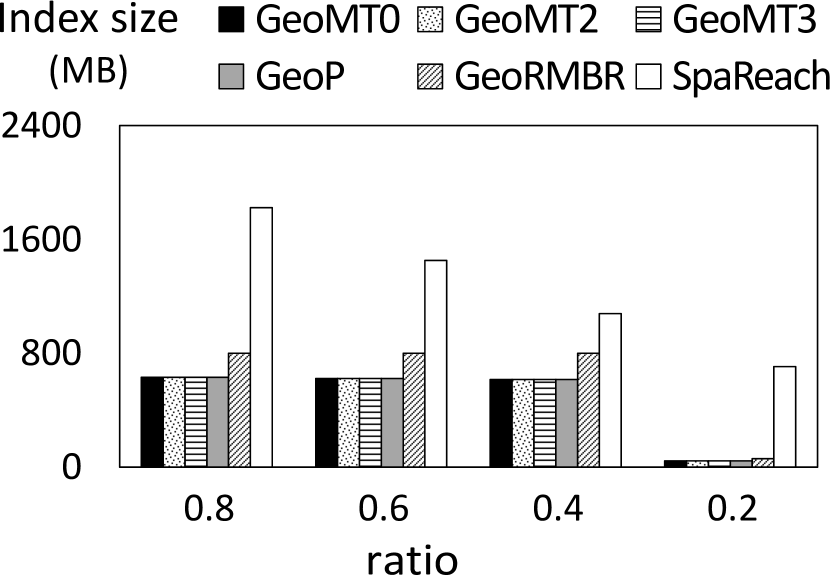
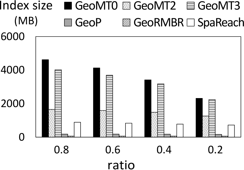
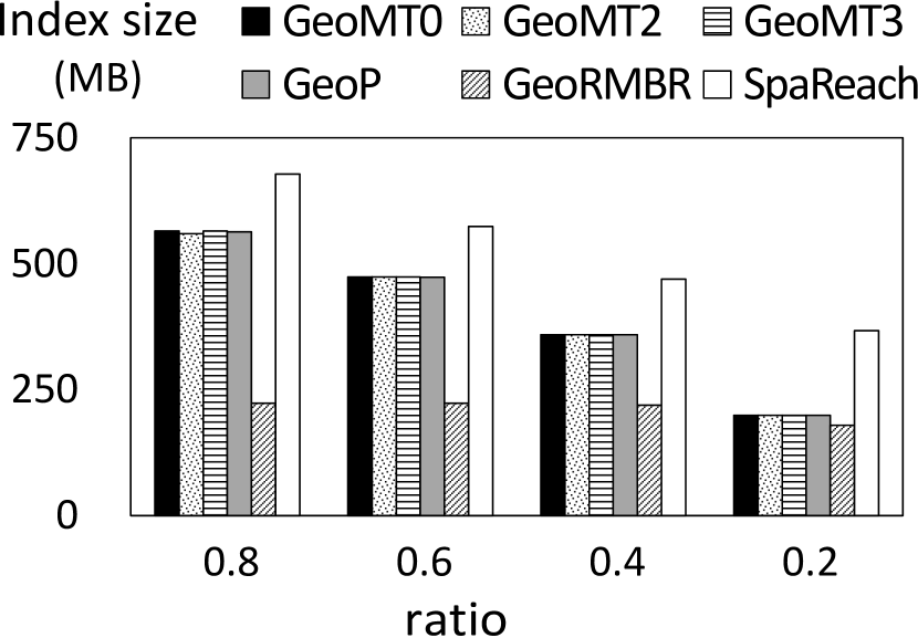
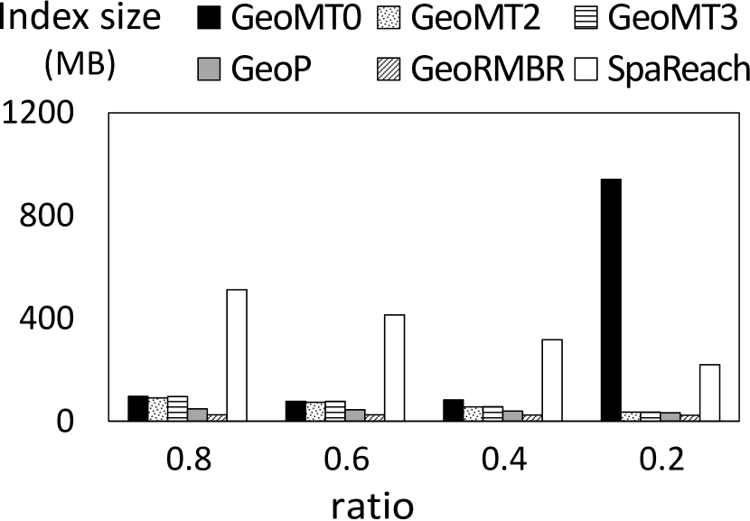
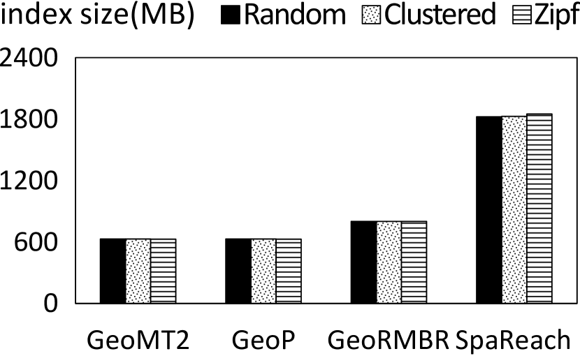
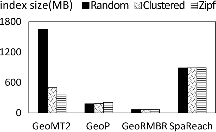
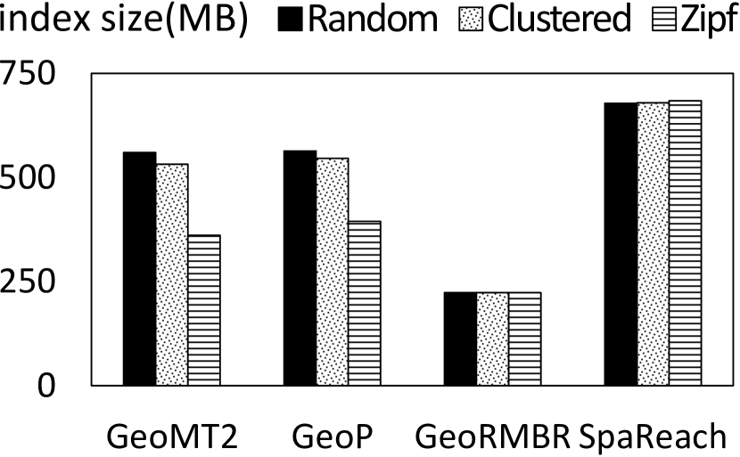
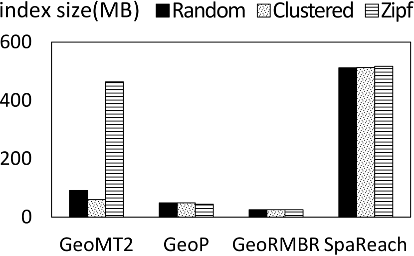
Figure 6(a) gives the storage overhead of all approaches for the uniprot150m dataset. In this experiment, the spatial vertices are randomly distributed in space. Since uniprot22m and uniprot100m share the same pattern with uniprot150m (even spatial distribution of vertices varies), they are not shown in the figure. The experiments show that GeoReach and all its variants require less storage overhead than SpaReach because of the additional overhead introduced by the spatial index. When there are less spatial vertices, SpaReach obviously occupies less space because size of spatial index lessens. However, SpaReach always requires more storage than any other approaches. Storage overhead of GeoReach approaches shows a two-stages pattern which means it is either very high (ratio = 0.8, 0.6 and 0.4) or very low (ratio = 0.2). The reason is as follows. These graphs are sparse and almost all vertices reach the same vertex. This vertex cannot reach any other vertex. Let us call it an end vertex. If the end vertex is a spatial vertex, then all vertices that can reach the end vertex will keep their spatial reachability information (no matter what category they are) in storage. But if it is not, majority of vertices will store nothing for spatial reachability information. GeoMT0 and GeoP are of almost the same index size because of sparsity and end-point phenomenon in these graphs. Such characteristic causes that almost each vertex can just reach only one grid which makes MAX_REACH_GRIDS invalid in approach GeoMT0 (number of reachable grids is always less than MAX_REACH_GRIDS) which makes GeoMT0 and GeoP have nearly the same size. For similar reason, MERGE_COUNT becomes invalid in these datasets which makes GeoMT2 and GeoMT3 share the same index size with GeoMT0 and GeoP. We also find out that index size of GeoRMBR is slightly larger than GeoMT0 approaches. Intuitively, RMBR should be more scalable than ReachGrid. But most of the vertices in these three graphs can reach only one grid. In GeoRMBR, for each vertex that have reachable spatial vertices, we assign an RMBR which will be stored as coordinates of RMBR’s top-left and lower-right points. It is more scalable to store one grid id than two coordinates. So when a graph is highly sparse, index size of GeoMT0 is possible to be less than GeoRMBR.

Figure 6(c) shows that in go-uniprot all GeoReach approaches performs better than SpaReach. When we compare all the GeoReach approaches, GeoMT0, GeoMT2 and GeoMT3 lead to almost the same storage overhead. That happens due to the fact that go-uniprot is a very sparse graph. A vertex can only reach few grids in the whole space. Grid cells in ReachGrid can hardly be spatially adjacent to each other which causes no integration. The graph sparsity makes the number of reachable grids in ReachGrid always less than MAX_REACH_GRIDS which leads to less R-vertices and more G-vertices. In consequence, go-uniprot, GeoMT0, GeoMT2, GeoMT3 and GeoP lead to the same storage overhead. It is rational that GeoRMBR requires the least storage because RMBR occupies less storage than ReachGrid.

When graphs are denser, results become more complex. Figure 6(b) shows index size of different approaches in patent dataset with randomly-distributed spatial vertices. GeoRMBR and GeoP, take the first and the second least storage and are far less than other approaches because both of them use RMBR which is more scalable. GeoMT0 takes the most storage in all spatial ratios for that ReachGrid takes high storage overhead. GeoMT2 and GeoMT3 require less storage than GeoMT0 because spatially-adjacent reachable grids in GeoMT0 are merged which brings us scalability. GeoMT3 are more scalable than GeoMT2 because MERGE_COUNT in GeoMT2 is 2 which causes more integration. There are three approaches, GeoMT3, GeoP and GeoRMBR, that outperform SpaReach approach. By tuning parameters in GeoReach, we are able achieve different performance in storage overhead and can also outperform SpaReach.

Figure 6(d) depicts index size of all approaches in citeseerx with randomly distributed spatial vertices. Spatial vertices ratio ranges from 0.8 to 0.2. All GeoReach approaches outperform SpaReach except for one outlier when spatial vertices ratio is 0.2. GeoMT0 consumes huge storage. This is caused by the center vertex which is above-mentioned. Recall that large proportion of ReachGrid contains almost all grids in space. After bitmap compression, it will cause low storage overhead. This is why when spatial vertices ratio is 0.8, 0.6 and 0.4, GeoMT0 consumes small size of index. When the ratio is 0.2, there are less spatial vertices. Although graph structure does not change, the center vertex reach less spatial vertices and less grids. Then the bitmap compression brings no advantage in storage overhead.

Figure 7 shows the impact of spatial data distribution on the storage cost. GeoMT0, GeoMT2 and GeoMT3 are all ReachGrid-based approaches. Spatial data distribution of vertices influences all approaches the same way. For all datasets, SpaReach is not influenced by the spatial data distribution. SpaReach consists of two sections: (1) The reachability index size is determined by graph structure and (2) The spatial index size is directly determined by number of spatial vertices. Hence, SpaReach exhibits the same storage overhead for different spatial data distributions. When spatial vertices distribution varies, GeoRMBR also keeps stable storage overhead. This is due to the fact that the storage overhead for each RMBR is a constant and the number of stored RMBR s is determined by the graph structure and spatial vertices ratio, and not by the spatial vertices distribution. Spatial data distribution can only influence the shape of each RMBR.

Figure 7(a) shows that each approach in GeoReach keeps the same storage overhead under different distributions in uniprot150m. As mentioned before, GeoMT0, GeoMT2, GeoMT3 and GeoP actually represent the same data structure since there is only a single reachable grid in ReachGrid. When there is only one grid reachable, varying the spatial distribution becomes invalid for all approaches which use ReachGrid.

Figure 7(b) and 7(c) shows that the storage overhead introduced by ReachGrid-based approaches decreases when spatial vertices become more congested. Randomly distributed spatial data is the least congested while zipf distributed is the most. The number of reachable spatial vertices from each vertex do not change but these reachable spatial vertices become more concentrated in space. This leads to less reachable grids in ReachGrid.

Figure 7(d) shows that when spatial vertices are more congested, ReachGrid based approaches, i.e., GeoMT0, GeoMT2 and GeoMT3, tend to be less scalable. Recall that citeseerx dataset is a polarized graph with a center vertex. One group contains vertices that can reach huge number of vertices (about 200,000) due to the center vertex. When spatial vertices are more concentrated and that will lead to more storage overhead.

(a) uniprot150

(b) patent

(c) go-uniprot

(d) citeseerx

Figure 8: Initialization time (Randomly distributed, spatial vertex ratio from 0.8 to 0.2)

VI-C Initialization time

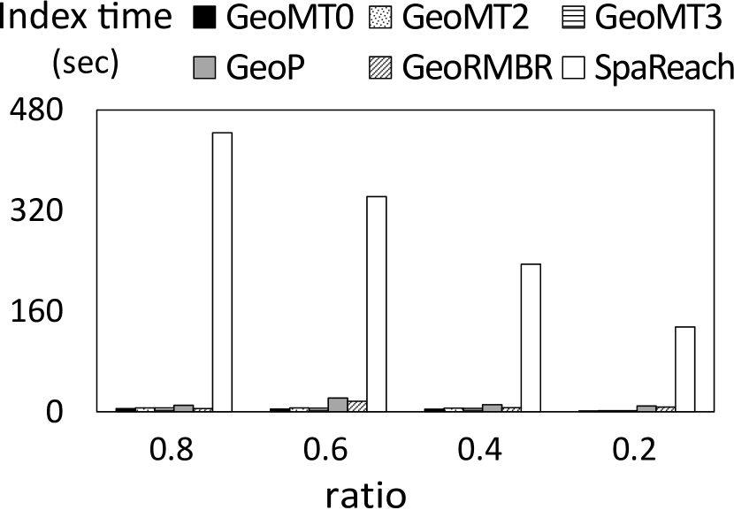
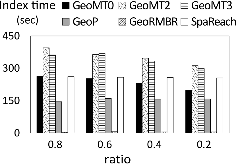
In this section, we evaluate the index initialization time for all considered approaches. For brevity, we only show the performance results for four datasets, uniprot150m, patent, go-uniprot and citeseerx, since uniprot22m, uniprot100m and uniprot150m datasets exhibit the same performance. Figure 8(a) shows that SpaReach requires much more construction time than the other approaches under all spatial ratios. Although these graphs are sparse, they contain large number of vertices. This characteristic causes huge overhead in constructing a spatial index which dominates the initialization time in SpaReach. Hence, SpaReach takes much more time than all other approaches. However, the SpaReach initialization time decreases when decreasing the number spatial vertices since the spatial index building step deals with less spatial vertices in such case. However, SpaReach remains the worst even when the spatial vertex ratio is set to 20%.

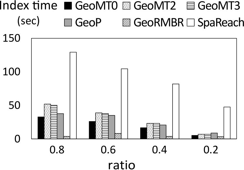
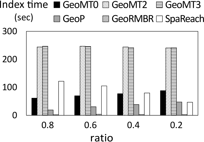
Figures 8(b) and 8(d) gives the initialization time for both the patent and citeseerx datasets, respectively. GeoRMBR takes significantly less initialization time compared to all other approaches. GeoP takes less time than the rest of approaches because it is ReachGrid of partial vertices whose number of reachable grids are less than MAX_REACH_GRIDS that are calculated. In most cases, GeoMT0 can achieve almost equal or better performance compared to SpaReach while GeoMT2 and GeoMT3 requires more time due to the integration of adjacent reachable grids. To sum up, GeoRMBR and GeoP perform much better than SpaReach in initialization even in very dense graphs. GeoMT0 can keep almost the same performance with SpaReach approach.

Figure 8(c) shows the initialization time for all six approaches on the go-uniprot dataset. Both RMBR approaches, i.e., GeoRMBR and GeoP, still outperform SpaReach. This is due to the fact that a spatial index constitutes a high proportion of SpaReach initialization time. As opposed to the uniprot150m case, the smaller performance gap between initializing GeoRMBR and SpaReach in go-uniprot.is explained as follows. The size of go-uniprotis far less than uniprot150m which decreases the spatial index initialization cost. As a result, the index construction time in SpaReach is less than that in uniprot150m. Since this graph has more reachability information, all GeoReach approaches require more time than in uniprot150m. It is conjunction of GeoReach and SpaReach index size changes that causes the smaller gap.

VII Conclusion

This paper describes GeoReach a novel approach that evaluates graph reachability queries and spatial range predicates side-by-side. GeoReach extends the functionality of a given graph database management system with light-weight spatial indexing entries to efficiently prune the graph traversal based on spatial constraints. GeoReach allows users to tune the system performance to achieve both efficiency and scalability. Based on extensive experiments, we show that GeoReach can be scalable and query-efficient than existing spatial and reachability indexing approaches in relatively sparse graphs. Even in rather dense graphs, our approach can outperform existing approaches in storage overhead and initialization time and still achieves faster query response time. In the future, we plan to study we plan to study the extensibility of GeoReach to support different spatial predicates. Furthermore, we aim to extend the framework to support a distributed system environment. Last but not least, we also plan to study the applicability of GeoReach to various application domains including: Spatial Influence Maximization, Location and Social-Aware Recommendation, and Location-Aware Citation Network Analysis.

References

- [1] R. Agrawal, A. Borgida, and H. V. Jagadish. Efficient Management of Transitive Relationships in Large Data and Knowledge Bases. ACM, 1989.
- [2] R. Bayer and E. M. McCreight. Organization and Maintenance of Large Ordered Indices. Acta Informatica, 1(3):173–89, 1972.
- [3] N. Beckmann, H.-P. Kriegel, R. Schneider, and B. Seeger. The R*-Tree: An Efficient and Robust Access Method for Points and Rectangles. In SIGMOD, pages 322–331, May 1990.
- [4] J. L. Bentley. Multidimensional Binary Search Trees Used for Associative Searching. Communications of the ACM, CACM, 18(9):509–517, 1975.
- [5] J. Cai and C. K. Poon. Path-hop: efficiently indexing large graphs for reachability queries. In CIKM, pages 119–128. ACM, 2010.
- [6] L. Chen, A. Gupta, and M. E. Kurul. Stack-based algorithms for pattern matching on dags. In VLDB, pages 493–504. VLDB Endowment, 2005.
- [7] Y. Chen and Y. Chen. An efficient algorithm for answering graph reachability queries. In ICDE, pages 893–902. IEEE, 2008.
- [8] J. Cheng, S. Huang, H. Wu, and A. W.-C. Fu. Tf-label: a topological-folding labeling scheme for reachability querying in a large graph. In SIGMOD, pages 193–204. ACM, 2013.
- [9] J. Cheng, S. Huang, H. Wu, and A. W.-C. Fu. Tf-label: a topological-folding labeling scheme for reachability querying in a large graph. In SIGMOD, pages 193–204. ACM, 2013.
- [10] J. Cheng, Z. Shang, H. Cheng, H. Wang, and J. X. Yu. K-reach: who is in your small world. PVLDB, 5(11):1292–1303, 2012.
- [11] J. Cheng, J. X. Yu, X. Lin, H. Wang, and P. S. Yu. Fast computing reachability labelings for large graphs with high compression rate. In EDBT, pages 193–204. ACM, 2008.
- [12] E. Cohen, E. Halperin, H. Kaplan, and U. Zwick. Reachability and distance queries via 2-hop labels. SIAM Journal on Computing, 32(5):1338–1355, 2003.
- [13] D. Comer. The Ubiquitous B-Tree. ACM Computing Surveys, 11(2):121–137, 1979.
- [14] R. A. Finkel and J. L. Bentley. Quad trees: A Data Structure for Retrieval of Composite Keys. Acta Informatica, 4(1):1–9, 1974.
- [15] J. E. Gonzalez, Y. Low, H. Gu, D. Bickson, and C. Guestrin. GraphChi: Large-Scale Graph Computation on Just a PC. In OSDI, 2012.
- [16] A. Guttman. R-Trees: A Dynamic Index Structure For Spatial Searching. In SIGMOD, 1984.
- [17] H. Jagadish. A compression technique to materialize transitive closure. TODS, 15(4):558–598, 1990.
- [18] R. Jin, Y. Xiang, N. Ruan, and H. Wang. Efficiently answering reachability queries on very large directed graphs. In SIGMOD, pages 595–608. ACM, 2008.
- [19] J. Liagouris, N. Mamoulis, P. Bouros, and M. Terrovitis. An effective encoding scheme for spatial RDF data. PVLDB, 7(12):1271–1282, 2014.
- [20] D. B. Lomet. Grow and Post Index Trees: Roles, Techniques and Future Potential. In SSD, pages 183–206, Aug. 1991.
- [21] P. Rigaux, M. Scholl, and A. Voisard. Spatial Databases with Application to GIS. Morgan Kaufmann, 2002.
- [22] H. Samet. The Design and Analysis of Spatial Data Structures. Addison-Wesley, 1990.
- [23] H. Samet. Foundations of Multidimensional and Metric Data Structures. Morgan Kaufmann, 2006.
- [24] M. Sarwat, S. Elnikety, Y. He, and G. Kliot. Horton: Online Query Execution Engine for Large Distributed Graphs. In ICDE, 2012.
- [25] M. Sarwat, S. Elnikety, Y. He, and M. F. Mokbel. Horton+: A Distributed System for Processing Declarative Reachability Queries over Partitioned Graphs. PVLDB, 6(14):1918–1929, 2013.
- [26] R. Schenkel, A. Theobald, and G. Weikum. Hopi: An efficient connection index for complex xml document collections. In EDBT, pages 237–255. Springer, 2004.
- [27] S. Seufert, A. Anand, S. Bedathur, and G. Weikum. Ferrari: Flexible and efficient reachability range assignment for graph indexing. In ICDE, pages 1009–1020. IEEE, 2013.
- [28] B. Shao, H. Wang, and Y. Li. Trinity: A Distributed Graph Engine on a Memory Cloud. In SIGMOD, 2013.
- [29] S. Shekhar and S. Chawla. Spatial Databases: A Tour. Prentice Hall, 2003.
- [30] S. Trißl and U. Leser. Fast and practical indexing and querying of very large graphs. In SIGMOD, pages 845–856. ACM, 2007.
- [31] S. J. van Schaik and O. de Moor. A memory efficient reachability data structure through bit vector compression. In SIGMOD, pages 913–924. ACM, 2011.
- [32] H. Wang, H. He, J. Yang, P. S. Yu, and J. X. Yu. Dual labeling: Answering graph reachability queries in constant time. In ICDE, pages 75–75. IEEE, 2006.
- [33] Y. Yano, T. Akiba, Y. Iwata, and Y. Yoshida. Fast and scalable reachability queries on graphs by pruned labeling with landmarks and paths. In CIKM, pages 1601–1606. ACM, 2013.
- [34] H. Yildirim, V. Chaoji, and M. J. Zaki. Grail: Scalable reachability index for large graphs. PVLDB, 3(1-2):276–284, 2010.
- [35] A. D. Zhu, W. Lin, S. Wang, and X. Xiao. Reachability queries on large dynamic graphs: a total order approach. In SIGMOD, pages 1323–1334. ACM, 2014.