Connecting inflation with late cosmic acceleration by particle production

Abstract

A continuous process of creation of particles is investigated as a possible connection between the inflationary stage with late cosmic acceleration. In this model, the inflationary era occurs due to a continuous and fast process of creation of relativistic particles, and the recent accelerating phase is driven by the non-relativistic matter creation from the gravitational field acting on the quantum vacuum, which finally results in an effective equation of state less than $-1$. Thus, explaining recent results in favor of a phantom dynamics without the need of any modifications in the gravity theory has been proposed. Finally, we confront the model with recent observational data of type Ia Supernova, history of the Hubble parameter, baryon acoustic oscillations, and the cosmic microwave background.

I Introduction

Recently, Planck Collaboration Planck has presented us with the most complete image of the early Universe. This provides strong constraints on the inflationary phase. In particular, the spectral index and the tensor-to-scalar ratio have been measured to be, $n_{s}=0.9603\pm 0.0073$ (68 $\%$ CL), and $r<0.10$ at a $95\%$ C.L. respectively If confirmed, it will lead to important consequences, particularly, many inflationary models may be ruled out by these bounds.

In the last few years, a large amount of observational data coming from Type Ia Supernovae (SNe Ia) Permutter ; Reiss11 , Cosmic Microwave Radiation Background (CMB) Spergel ; ade and Large Scale Structure (LSS) Daniel ; Percival reveal that the universe is currently undergoing through an accelerated expansion. A crucial quantity in the models based on Einstein gravity aimed at accounting for this expansion is the equation of state (EoS) of dark energy (DE), i.e., $w_{de}=p_{de}/\rho_{de}$, the ratio of the pressure to the energy density of the dark energy. In the case of the Lambda cold dark matter, $\Lambda$CDM model, this agent can be identified with the energy of the quantum vacuum whence the corresponding EoS parameter is just $w_{\Lambda}=-1$. In spite of the observational success of this model, recent model-independent measurements of $w_{de}$ seem to favor a slightly more negative EoS (see, e.g., Refs. Rest ; Xia ; Cheng ; Shafer ), which, if confirmed, would invalidate the model. In particular, the Planck mission yields $w_{de}=-1.13^{+0.13}_{-0.10}$ ade , Rest et al., using supernovae type Ia (SN Ia) data from the Pan-STARRS1 Medium Deep Survey found $w_{de}=-1.166^{+0.072}_{-0.069}$, i.e., $w_{de}<-1$ at 2.3 $\sigma$ confidence level Rest , Shafer and Huterer Shafer using geometrical data from SN Ia, baryon acoustic oscillations (BAOs), and CMB, determined $w_{de}<-1$ at 2$\sigma$ confidence level. The simplest way to get $w_{de}<-1$, consistent with general relativity, is assume that the DE has your origin at a phantom field Caldwell . Despite being compatible with observational data, such a possibility has serious theoretical problems Carroll ; Cline ; Hsu ; Sbisa ; Dabrowski . Other stringent constraints on the EoS have been analyzed in several contexts, such as, considering a variable EoS for both dark components Kumar , using cosmographic methods to investigate various dynamic EoS models Aviles , and a reconstruction of the dark energy EoS via node-based reconstruction Vazquez .

In a recent work Dr1 , the authors investigated an alternative to this possibility, namely, that the measured equation of state, $w_{de}$, is in reality an effective one, the equation of state of the quantum vacuum, $w_{\Lambda}=-1$, plus the negative equation of state, $w_{c}$, associated to the production of particles by the gravitational field acting on the vacuum. From a joint analysis of data Supernova type Ia, gamma ray bursts, baryon acoustic oscillations, and the Hubble rate, it was obtained that $w_{eff}(z=0)=-1.155^{+0.076}_{-0.080}$ at 1$\sigma$.

In this context, one may wonder that the primeval accelerated expansion of the universe (i.e., the inflationary era) could result in a very fast rate of relativistic particle productions due to action of the gravitational field on the quantum vacuum. If for a sufficiently long period of time, this rate was high enough to compensate, or nearly compensate, for the dilution of particles due to the universe expansion, then the energy density of the particles fluid wound remain nearly constant giving rise to an inflationary expansion. To the best of our knowledge, this idea was first proposed in Turok .

It is important to mention that inflation driven by the particle production is not a new subject. Particle creation as a source of inflation in the early Universe, was first investigated in Starobinsky1 , using the expressions for the energy-momentum of the created particles and the rate of their creation ($\propto R^{2}$ for non-conformal particles in a FLRW universe) derived earlier in Starobinsky2 . However, it appeared that such model presents some problems, such as, they can not produce a sufficiently low curvature during inflation, and a graceful exit from it. Thus, success in constructing viable inflationary models was achieved in the Starobinsky model Starobinsky3 in which the dissipation and the creation of matter occurred already after the end of inflation. However, the idea of particle creation driving inflation was revived after that under the name of warm inflation warm_inflation . The aim of this paper is to explore a possible connection between the inflationary stage with late cosmic acceleration through of a continuous process of creation of particles by the gravitational field acting on the quantum vacuum ccdm_inflation .

This paper is organized as follows. The next section briefly sums up the phenomenological basis of particle creation in an expanding homogeneous and isotropic, spatially flat, universe. In section III, we describe the inflationary era as a result of a continuous and fast process of creation of relativistic particles. In section III, we present the dynamics of the universe in the post inflationary era in presence of a continuous matter creation associated with the production of particles by the gravitational field acting on the vacuum. Section V specifies the various sets of data and the statistical analysis employed to constrain the model. The concluding section summarizes and gives comments on our findings. As usual, the scale factor of the Friedmann-Robertson-Walker (FRW) metric is normalized so that $a_{0}=1$, the naught subscript indicates the present time.

II Cosmological models with particle creation

As investigated by Parker and collaborators Parker , the material content of the Universe may have had its origin in the continuous creation of radiation and matter from the gravitational field of the expanding cosmos acting on the quantum vacuum, regardless of the relativistic theory of gravity assumed. In this picture, the produced particles draw their mass, momentum and energy from the time-evolving gravitational background which acts as a “pump” converting curvature into particles.

Prigogine Prigogine studied how to insert the creation of matter consistently in Einstein’s field equations. This was achieved by introducing in the usual balance equation for the number density of particles, $(n\,u^{\alpha})_{;\alpha}=0$, a source term on the right hand side to account for the production of particles, namely,

$$(n\,u^{\alpha})_{;\alpha}=n\Gamma\,,$$ (1)

where $u^{\alpha}$ is the particle fluid four-velocity normalized so that $u^{\alpha}\,u_{\alpha}=1$, and $\Gamma$ denotes the particle production rate. According to Parker’s theorem, the production of relativistic particles is strongly suppressed in the radiation era Parker-Toms . The above equation, when combined with the second law of thermodynamics, naturally leads to the appearance of a negative pressure, the creation pressure $p_{c}$, which adds to the other pressures (i.e., radiation, baryons, dark matter, and vacuum pressure) in the stress-energy tensor. These results were subsequently discussed and generalized in Lima1 , mnras-winfried , and Zimdahl by means of a covariant formalism, and were further confirmed by using relativistic kinetic theory cqg-triginer ; Lima-baranov .

Since the entropy flux vector of matter, $n\sigma u^{\alpha}$, where $\sigma$ denotes the entropy per particle, must fulfill the second law of thermodynamics $(n\sigma u^{\alpha})_{;\alpha}\geq 0$, the constraint $\Gamma\geq 0$ readily follows.

For a homogeneous and isotropic universe, with scale factor $a$, in which there is an adiabatic process of particle production from the quantum vacuum, a direct relationship between the creation pressure and the particle production rate exists as Lima1 ; Zimdahl

$$p_{c}=-\frac{\rho\,+\,p}{3H}\,\Gamma\,.$$ (2)

Therefore, being $p_{c}$ negative, it may have produced the accelerated expansion in the early Universe (i.e., inflationary era), as well as, it may also drive the present accelerated cosmic expansion. Here, $\rho$, $p$, respectively, denote the energy density and the pressure of the corresponding fluid, $H=\dot{a}/a$ is the Hubble factor, and as usual, an overdot denotes the differentiation with respect to cosmic time.

The EoS associated with the process of creation of matter follows from Eq. (2)

$$w_{c}=-(1+w)\frac{\Gamma}{3H},$$ (3)

where $w=0$ for non-relativistic matter, and $w=1/3$ for relativistic matter.

III The inflationary epoch

We consider a spatially-flat Friedmann-Robertson-Walker (FRW) universe, with Hubble factor $H(t)= ̇\dot{a}(t)/a(t)$. We assume a universe undergoing a continuous process of particle creation thanks to the action of the gravitational field on the quantum vacuum. The first Friedmann equation reads

$$H^{2}=\frac{1}{3M^{2}_{pl}}\rho,$$ (4)

where $M_{pl}=(8\pi G)^{-1/2}$ is the reduced Planck mass.

Let us consider the possibility that the early inflationary phase was the result of a continuous and fast process of creation of particles, so fast that the energy density $\rho$ stays practically constant by about 55 e-folds, to decline quickly afterwards around the GUT era.

To go ahead, an expression for the rate $\Gamma$ is needed. We first assume that the total rate split into two terms as

$$\Gamma=\Gamma_{r}+\Gamma_{dm},$$ (5)

with $\Gamma_{r}$ referring to the particle creation rate in the early universe, and $\Gamma_{dm}$, the particle creation rate of dark matter particles. Then we adopt the following phenomenological expressions

$$\Gamma_{r}=3H\xi\exp[-(\alpha a^{n})],$$ (6)

and

$$\Gamma_{dm}=3H\beta[1-\tanh(10-12a)],$$ (7)

where, $\xi$, $\alpha$, $n$, and $\beta$ are positive constant parameters. The parameter $n$ is associated with the decay rate of the particle production. The higher $n$, the faster $\Gamma_{r}$ goes down. Thus, in order to obtain an inflationary expansion for a sufficiently long period of time, $n$ must lie in an interval $0.10\leq n\leq 0.12$. Here, we adopt $n=0.10$. For other values within the above range, the dynamics generated by $\Gamma_{r}$ is practically the same. Let us consider $\xi=3/4$, to eliminate the possibility of an EoS less than $-1$ in the inflationary era. The constants $\alpha$, $\beta$ are free parameters of the model to be constrained by the observational data. When $a\rightarrow 0$, $\Gamma_{dm}$ gets close to zero regardless the value of $\beta$. In fact, as we will see later, $\Gamma_{dm}$ practically does not influence the cosmic dynamics for $a\geq 0.6$, since in the very early universe, the production of non relativistic matter is negligible. Figure 1 shows the ratio $\Gamma_{r}/3H$ in terms of the scale factor for different values of $\alpha$. From Eqs. (5) – (7), it is seen that at early times ($a\ll 1$) $\Gamma\simeq\Gamma_{r}$, and $\Gamma\simeq\Gamma_{dm}$, otherwise.

Let us assume that the dynamics of the very early universe was dominated by a production of particles given by Eq. (6). At the end of this phase, the scale factor will have grown enormously, the production of particles will have declined sharply, and the transition to the radiation dominated phase occurs. According to Parker’s theorem, in the latter phase massless particles cannot be quantum-mechanically produced Parker-Toms .

The dynamics of the early inflationary era is usually described by a self-interacting scalar field, $\phi$, that slowly rolls down its potential, $V(\phi)$, in such a way that the latter dominates the total energy density (i.e., $\dot{\phi^{2}}/2\ll V(\phi)$) during the inflationary expansion. It is therefore illustrative to relate $w_{c}$ to a scalar field that would generate the same amount of inflation as the particle production scenario.

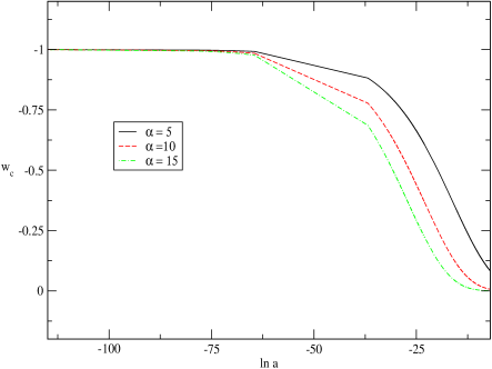
Figure 1: Evolution of $w_{c}$ for different values of the parameter $\alpha$.

Since $\rho_{\phi}+p_{\phi}=\dot{\phi^{2}}$, and it must be equal to $\rho_{r}+p_{r}$, it follows that $\dot{\phi}^{2}=\rho_{r}(1+w_{c})$, where $\rho_{r}$ represents the energy density of the relativistic matter.

Hence,

$$\frac{d\phi}{da}=\frac{1}{aH}\sqrt{\rho_{r}(1+w_{c})}.$$ (8)

Accordingly,

$$\Delta\phi=\int\frac{da}{aH}\sqrt{\rho_{r}(1+w_{c})}.$$ (9)

As a consequence, the total variation of the scalar field during inflation is

$$\frac{\Delta\phi}{M_{pl}}\simeq\sqrt{3}\sqrt{\Big{[}1+w_{c}\Big{]}}N,$$ (10)

where $N=\ln\Big{(}\frac{a_{end}}{a_{i}}\Big{)}$ is the total number of e-folds produced during inflation. Generically, total number of e-folds should be about 60 in order to solve the flatness and horizon problem of the standard big bang theory. In fact, the spectrum of fluctuations observed in the CMB corresponds to the values of $N$ in the interval $50\leq N\leq 60$ Planck .

Figure 2 shows $N$ as a function of $w_{c}$ for different values of $\Delta\phi$. Note that, to produce a suitable number of e-folds, we must have $w_{c}\simeq-1$. This is possible provided, $0<\alpha\leq 10$ (see Fig. 1). The number of e-folds $N$ before the end of inflation is related to the variation of scalar field by

$$dN=-Hdt=\frac{1}{\sqrt{2\epsilon}M_{pl}}d\phi,$$ (11)

where $\epsilon=\frac{M^{2}_{pl}}{2}\Big{(}\frac{1}{V}\frac{dV}{d\phi}\Big{)}^{2}$ is a dimensionless slow-roll parameter. The accelerated expansion occurs so long as $\epsilon\ll 1$. For later use, we recast the above equation as

$$\epsilon=\frac{1}{2}\Big{[}\frac{d}{dN}\Big{(}\frac{\Delta\phi}{M_{pl}}\Big{)}\Big{]}^{2}.$$ (12)

An obvious condition for the slow-roll is that $\ddot{\phi}<<H\dot{\phi}$. This requires that the so-called second slow-roll parameter, $\eta\equiv\epsilon-\frac{1}{H}\frac{1}{2\epsilon}\frac{d\epsilon}{dt}$, be much less than unity. This implies,

$$\eta=\epsilon-\frac{1}{2\epsilon}\frac{d\epsilon}{dN}\ll 1.$$ (13)

During slow-roll regime, $\epsilon\ll 1$ and $\mid\eta\mid\ll 1$. From Eqs. (12) and (10), it follows

$$\epsilon=\frac{3}{2}\Big{(}1+w_{c}\Big{)},$$ (14)

and $\eta=\epsilon$.

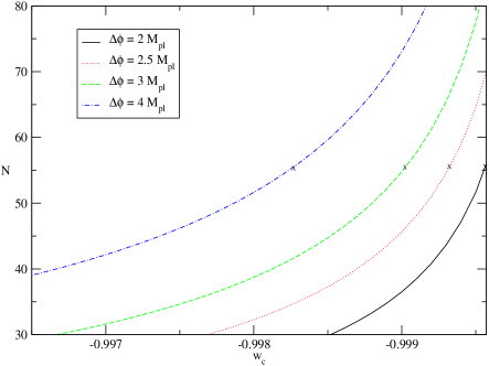
Figure 2: Number of e-folds as a function of $w_{c}$.

A further important parameter related to the inflationary behavior is the tensor-to-scalar ratio $r$, which quantifies the ratio between the scalar and tensor spectra of the fluctuations produced in the inflationary era. During the slow-roll, $r$ does not evolve much and one may recover Lyth bound Lyth which relates $r$ to the total field excursion during inflation

$$\frac{\Delta\phi}{M_{pl}}\simeq\Big{(}\frac{r}{0.01}\Big{)}^{1/2}.$$ (15)

From Eq. (10), we have

$$r=3\times 10^{-2}\,N^{2}\,\Big{(}1+w_{c}\Big{)}.$$ (16)

Considering $N=55$ (see Figure 2), we obtain $r$ = 0.163, 0.090, 0.062, and 0.045, respectively, for $\Delta\phi=4M_{pl}$, $\Delta\phi=3M_{pl}$, $\Delta\phi=2.5M_{pl}$, and $\Delta\phi=2M_{pl}$. In the slow-roll approximation, keeping in mind that $\epsilon=\eta$ for the model presented in this work, we have $r\simeq 8(1-n_{s})$. Thus, we get $n_{s}\simeq 0.959,0.977,0.984$, and 0.988, for $\Delta\phi=4M_{pl}$, $\Delta\phi=3M_{pl}$, $\Delta\phi=2.5M_{pl}$, and $\Delta\phi=2M_{pl}$, respectively. The Planck collaboration obtained $r<0.11$ (95 $\%$ CL), and $n_{s}=0.968^{+0.006}_{-0.006}$ (68 $\%$ CL).

The model presented in this section for the particle creation rate in the very early universe given by Eq. (6) is in good agreement with the observational data recently released by the Planck collaboration Planck . The dynamical consequences of the second term in Eq.(5), $\Gamma_{dm}$, that gives the production rate of density matter particles, will be considered in section IV.

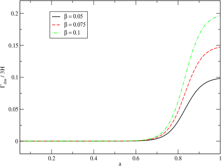
Figure 3: Evolution of ratio $\Gamma_{dm}/3H$. In drawing the graphs, we have taken $\beta=0.050$, 0.075 and 0.1, for the solid, dashed, and dot-dashed line, respectively.

IV The post inflationary era

Let us now consider a spatially flat FRW universe dominated by pressureless matter (baryonic plus dark matter) and the energy of the quantum vacuum (the latter with EoS $p_{\Lambda}=-\rho_{\Lambda}$) in which a process of dark matter creation from the gravitational field, governed by

$$\dot{\rho}_{dm}\,+\,3H\rho_{dm}=\rho_{dm}\,\Gamma_{dm},$$ (17)

is taking place. Since the production of ordinary particles is much limited by the tight constraints imposed by local gravity measurements ellis ; peebles_ratra ; Hagiwara , and radiation has practically negligible impact on the recent cosmic dynamics, hence, for the sake of simplicity, we assume that the produced particles are just dark matter particles. In writing the last equation, we used Eq. (1) specialized to dark matter particles and the fact $\rho_{dm}=n_{dm}\,m$, where $m$ stands for the rest mass of a typical dark matter particle. Figure 3 shows the evolution of $\Gamma_{dm}/3H$ defined in Eq. (7) up to present moment ($a_{0}=1$) for different values of $\beta$. In particular, for $\beta=0.1$ (shown in the dot-dashed line), we find that, at $a=0.1$, $\Gamma_{dm}/3H\simeq 10^{-9}$; $a=0.4$, $\Gamma_{dm}/3H\simeq 10^{-5}$; $a=0.7$, $\Gamma_{dm}/3H\simeq 10^{-2}$; and finally, at $a_{0}=1$, $\Gamma_{dm}/3H\simeq 0.1951$.

Since baryons are neither created nor destroyed, their corresponding energy density obeys $\dot{\rho}_{b}\,+\,3H\rho_{b}=0$. On the other hand, as the energy of the vacuum does not vary with expansion, so $\,\rho_{\Lambda}={\rm constant}$.

In this scenario the total pressure is $\,p_{\Lambda}\,+\,p_{c}$, thereby the effective EoS is just the sum of the EoS of vacuum plus that due to the creation pressure,

$$w_{eff}=-1\,-\frac{\Gamma}{3H}\,.$$ (18)

Since, by the second law of thermodynamics, $\Gamma$ is positive-semidefinite, we have that the effective EoS can be less than $-1$ without the need of invoking any scalar field with wrong sign in the kinetic term. Therefore, due to the combined effects of the vacuum and creation pressures, one can hope for a global EoS less that $-1$ without the need of any phantom fields. We mention that, an equation of state $w_{de}<-1$, without any introduction of phantom fields was first realized in the context of modified gravity models Boisseau , more specifically in the scalar-tensor theory of gravity. However, it is worth to recall that, we obtain this phantom behavior without any modifications in the gravitational theories, rather by the mechanism of gravitational particle productions in an adiabatic manner. We note that, particle creation in an expanding universe has been discussed to understand several aspects of modern cosmology. Recently, the authors in Refs. Capozziello ; Pereira ; Singh investigated the particle production rate in the context of $f(R)$ gravity. On the other hand, the possible effects of this mechanism have also been analyzed in case of a flat and negative curved FRW universes as well Montani .

Friedmann’s equation for this scenario is,

$$H^{2}=\frac{8\pi G}{3}(\rho_{b}\,+\,\rho_{dm}\,+\,\rho_{\Lambda}).$$ (19)

Inserting (7) in (17), and integrating, we have

$$\rho_{dm}=\rho_{dm0}\,a^{-3}\,\exp\Big{(}3\beta\int_{1}^{a}\frac{k(\tilde{a})}{\tilde{a}}d\tilde{a}\Big{)},$$ (20)

where $k(a)=\Gamma_{dm}/3H=\beta[1-\tanh(10-12a)]$.

In terms of the redshift, $z=a^{-1}-1$, the Hubble expansion rate reads

$$\frac{H^{2}(z)}{H^{2}_{0}}=\Omega_{b0}\,(1+z)^{3}$$

$$+\,\Omega_{dm0}\,(1+z)^{3}\,\exp\Big{(}-3\beta\int_{0}^{z}\frac{k(\tilde{z})}{(1+\tilde{z})}d\tilde{z}\Big{)}\,+\,\Omega_{\Lambda 0},$$ (21)

where the $\Omega_{i0}$ denote the current fractional densities of baryons, dark matter and vacuum, respectively.

V DATA SETS AND STATISTICAL ANALYSES

We first describe the set of data used in the statistical analysis. To constrain the free parameters $\theta_{i}=\{\beta,\Omega_{dm0}\}$ of the particle creation model, we use the following sets of data: a) The most recent Type Ia Supernovae (SNe Ia) data sets from the joint light-curve analysis (JLA) snia ; b) Baryon acoustic oscillations (BAO) data from the SDSS Luminous Red Galaxy sample Blake , the WiggleZ Survey Percival and 6dF Galaxy Survey Beutler ; c) Measurements of the Hubble function $H(z)$ compiled in Hz , plus data by the BOSS collaboration BOSS , $H(z=2.34)=222\pm 7$ km $s^{-1}$ Mpc. Their best fit values, with their corresponding 1$\sigma$ uncertainties are presented in subsection V.4. These follow from minimizing the likelihood function $L\propto\exp(-\chi_{total}^{2})$ with $\chi_{total}^{2}=\chi_{SNIa}^{2}+\chi_{BAO/CMB}^{2}+\chi_{H}^{2}$, where each $\chi^{2}_{i}$ (specified below) quantifies the discrepancy between theory and observation. The statistical analysis used for those observables is described in the following subsections.

V.1 Supernovae type Ia

SNe Ia are very bright standard candles, useful for measuring cosmological distances. Here, we use the JLA compilation consisting of 740 well-calibrated SNe Ia in the redshift range $z\in[0.01,1.30]$ snia . This collection of SNe Ia includes about 100 low-redshift SNe from a combination of various subsamples, $\sim$ 350 from SDSS at low to intermediate redshifts, $\sim$ 250 from SNLS at intermediate to high redshifts, and $\sim$ 10 high-redshift SNe from the Hubble Space Telescope. All of the SNe Ia have light curves of high quality, so their distance moduli can be obtained accurately. These data points are the most recent SNe Ia present in the literature.

The distance modulus predicted for a given supernova of redshift $z$ can be expressed as

$$\mu(z,\theta_{i})=5\log_{10}\Big{[}\frac{d_{L}(z,\theta_{i})}{Mpc}\Big{]}+25$$ (22)

where $d_{L}=(1+z)H_{0}\int_{0}^{z}\frac{dz^{\prime}}{H(z^{\prime})}$ is the luminosity distance.

The corresponding $\chi^{2}$ is then calculated in the usual way for correlated observations:

$$\chi^{2}_{SNIa}=\Delta\mu^{{\dagger}}C^{-1}\Delta\mu,$$ (23)

where $\Delta\mu=\mu_{obs}-\mu_{th}(\theta_{i})$ is the vector of differences between the observed, corrected distance moduli and the theoretical predictions that depend on the set of cosmological model parameters $\theta_{i}$, and $C$ is the covariance matrix for the observed distance moduli. The latter can be found in snia .

V.2 Baryon acoustic oscillations and cosmic microwave background

Here, we use a more model-independent constraint derived from the product of the acoustic scale of the cosmic microwave background (CMB), $l_{A}=\pi d_{A}(z_{*})/r_{s}(z_{*})$, and the measurement of the ratio of the sound horizon scale at the drag epoch and the BAO dilation scale, $r_{s}(z_{d})/D_{V}(z_{BAO})$, defined as $X=\frac{d_{A}(z_{*})}{D_{V}(z_{BAO})}\frac{r_{s}(z_{d})}{r_{s}(z_{*})}$. Here, $D_{V}(z)=[d^{2}_{A}(z)cz/H(z)]^{1/3}$ is the dilation scale introduced in Daniel , $d_{A}(z_{*})$ is the comoving angular-diameter distance to recombination $d_{A}(z_{{}_{*}})=c\int_{0}^{z_{*}}\frac{dz^{\prime}}{H(z^{\prime})}$, and $r_{s}(z_{*})$ is the comoving sound horizon at decoupling

$$r_{s}(z_{*})=\frac{c}{\sqrt{3}}\int_{0}^{1/(1+z*)}\frac{da}{a^{2}H(a)\sqrt{1+(3\Omega_{b0}/4\Omega_{\gamma 0})}}.$$ (24)

Inserting the ratio $r_{s}(z_{d})/r_{s}(z_{*})=1.044\pm 0.019$, with $z_{d}=1020$ and $z_{*}=1091$ Bennett , in the above equation for $X$, we obtain the BAO/CMB constraints

$$X=\frac{d_{A}(z_{*})}{D_{V}(z_{BAO})}.$$ (25)

We write the $\chi^{2}$ for the BAO/CMB analysis as

$$\chi^{2}_{BAO/CMB}=\Delta X^{{\dagger}}C^{-1}\Delta X,$$ (26)

where $\Delta X=X_{obs}-X_{th}(\theta_{i})$, and $C^{-1}$ is the inverse covariance matrix obtained in Giostri . Here we make use of the six data point compiled by R. Giostri et al. Giostri .

V.3 History of the Hubble parameter

The differential evolution of early-type passive galaxies provides direct measurements of the Hubble parameter, $H(z)$. An updated compilation of such data was presented in Hz . We adopt 28 data points in the redshift range $0.09<z<1.75$ reported in Hz , plus data from the BOSS colaboration BOSS , $H(z=2.34)=222\pm 7$ km $s^{-1}$ Mpc, to constrain the free parameters $\theta_{i}$. We compute the $\chi^{2}_{H}$ function defined as

$$\chi^{2}_{H}(\theta_{i},H_{0})=\sum_{i=1}^{28}\frac{[H^{obs}(z_{i})-H^{th}(z_{i},H_{0},\theta_{i})]^{2}}{\sigma^{2}_{H}(z_{i})},$$ (27)

where $H_{th}(z_{i},H_{0},\theta_{i})$ is the model-predicted value of the Hubble parameter at the redshift $z_{i}$. The present value of the Hubble parameter $H_{0}$ is marginalized.

V.4 Statistical results

Figure 4 shows the 68 $\%$ and 95$\%$ confidence contours in the $\Omega_{dm0}-\beta$ plane. During the statistical analysis is taken with physical condition which $\beta\geq 0$. We obtain as best fit for the model, $\beta=0.018^{+0.134}_{-0.151}$ and $\Omega_{dm0}=0.242^{+0.018}_{-0.014}$ at 1$\sigma$ confidence level (CL). Although the best fit for $\beta$ is small, the possibility of a small creation rate ($\beta>0\rightarrow\Gamma>0$) not can be ruled out. In fact, $0<\beta<0.1523$ and $0<\beta<0.2328$ at 1$\sigma$ and 2$\sigma$ CL, respectively. Figure 5 shows the reconstruction of the effective EoS in terms of scale factor. Note that $w_{eff}(a=1)=-1.053^{+0.053}_{-0.397}$, i.e, $w_{eff}<-1$ without the need of invoking phantom fields.

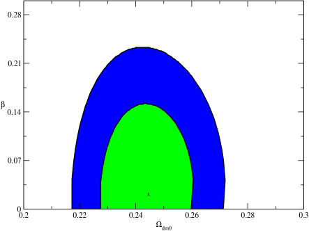
Figure 4: 1$\sigma$ and 2$\sigma$ confidence regions from joint analysis SNIa+BAO/CMB+$H(z)$.

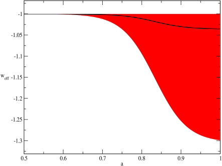
Figure 5: Evolution of the effective EoS; the solid (black) line indicates the best fit value, and the shaded region (red) the 1$\sigma$ uncertainty.

VI Conclusions

As shown by Parker and collaborators, the particle creation is something expected in expanding spacetime Parker . In spite of the difficulty in deriving the production rate, this phenomenon may in principle be related with inflation and the present cosmic acceleration ccdm_model .

However, the particle creation processes, during the very rapid early expansion of the universe, are believed to give rise to temperature anisotropies in the cosmic microwave background. Within of the context of a continuous matter creation process in an expanding universe, the effects on the CMB TT and EE power spectra were first investigated recently in eu_pan . In the cosmological context, CMB can be a powerful source to investigate the properties of an adiabatic matter creation process to strengthen the cosmological models driven by the adiabatic particle productions both for early and late universe.

We have shown here that in the limit of high energies, the production of relativistic particles from the vacuum leads to a viable inflationary solution, and this dynamics is in good agreement with the observational data recently released by the Planck collaboration Planck . Further, we present an alternative to the recently reported values of the dark energy equation of state beyond $-1$, may arise from the joint effect of the quantum vacuum and the process of particle production. This offers a viable alternative to the embarrassing possibility of the scalar fields which violate the dominant energy condition, and give rise to classical and quantum instabilities, and further do not respect the second law of thermodynamics.

Summarizing, by proper choice of the particle creation rate, the cosmic scenario presented in this work shows the evolution of the universe starting from the early inflationary era to the present accelerating phase, considering a continuous matter creation process by the gravitational field. Obviously, phenomenological models of particle production different from the ones essayed here are also worth exploring. However, the most important thing, from which the cosmological scenarios could be viewed more clearly, is to determine the production rate $\Gamma$ using quantum field theory in curved spacetimes.

- (1) Planck Collaboration, Planck 2015 results. XX. Constraints on inflation, arXiv:1502.02114 [astro-ph.CO].
- (2) Perlmutter, S. J., et al.: Astrophys. J. 517, 565 (1999).
- (3) Reiss, A.G., et al.: Astron. J. 116, 1009 (1998).
- (4) Spergel, D.N., et al.: Astrophys. J. Suppl. Ser. 170, 377 (2007)
- (5) P.A.R. Ade et al., [Planck Collaboration], “Planck 2013 results. XVI. Cosmological parameters”, Astron.& Astrophys. (in the press), arXiv:1303.5076[astro-ph.CO].
- (6) Eisenstein, D.J., et al.: ApJ 633, 560 (2005).
- (7) Percival, W.J., et al.: MNRAS 401, 2148 (2010).
- (8) A. Rest et al., ” Cosmological constraints from measurements of type Ia supernovae discovered during the first years of the Pan-STARRS1 Survey ”, Astrophys. J. (in press), arXiv:1310.3828[astro-ph.CO].
- (9) J.-Q. Xia, H. Li, and X. Zhang, Phys. Rev. D 88, 063501 (2013).
- (10) C. Cheng, and Q.-G Huang, Phys. Rev. D 89, 043003 (2014).
- (11) D.L. Shafer and D. Huterer, Phsy. Rev. D 89, 063510 (2014).
- (12) R.R. Caldwell, Phys. Lett. B 545, 23 (2002).
- (13) S.M. Carroll, M. Hoffman and M. Trodden, Phys. Rev. D 68, 023509 (2003).
- (14) J.M. Cline, S. Jeon and G. D. Moore, Phys. Rev. D 70, 86 043543 (2004).
- (15) S.D.H. Hsu, A. Jenkins, and M.B. Wise, Phys. Lett. B 597, 270 (2004).
- (16) F. Sbisa, “Classical and quantum ghosts”, arXiv:14.06.4550.
- (17) M. Dabrowski, “Puzzles of the dark energy in the universe - phantom”, arXiv: 1411.2827.
- (18) S. Kumar and L. Xu, Phys. Lett. B 737 244-247 (2014).
- (19) A. Aviles, C. Gruber, O. Luongo, and H. Quevedo, Phys. Rev.D 86, 123516 (2012).
- (20) J. A. Vazquez, M. Bridges, M. P. Hobson, and A. N.Lasenby, J. Cosmol. Astropart. Phys. 1209 020 (2012).
- (21) Rafael C. Nunes and Diego Pavón, Phys. Rev. D 91, 063526 (2015). arXiv:1503.04113v1 [gr-qc].
- (22) N. Turok, Phys. Rev. Lett., 60, 549 (1988).
- (23) V. T. Gurovich and A. A. Starobinsky, JETP 50, 844 (1979).
- (24) Ya. B. Zeldovich and A. A. Starobinsky, JETP 34, 1159 (1972); Ya. B. Zeldovich and A. A. Starobinsky, JETP Lett. 26, 252 (1977).
- (25) A. A. Starobinsky, Phys. Lett. B 91, 99 (1980).
- (26) A. Berera, Phys. Rev. Lett. 75, 3218 (1995).
- (27) L. R. W. Abramo and J. A. S. Lima, Class. Quant. Grav. 13 2953-2964 (1996); E. Gunzig, R. Maartens, and A. Nesteruk, Class. Quant. Grav 15 923-932 (1998); W. Zimdahl, Phys. Rev. D 61, 083511 (2000).
- (28) L. Parker, Fund. Cosm. Phys. 7, 201 (1982); L. Parker, Phys. Rev. Lett., 21, 562 (1968); L. Parker, Phys. Rev. Lett. 183, 1057 (1966); S.A. Fulling, L. Parker, and B.L. Hu, Phys. Rev. D, 10, 3905 (1974); L. Parker, Phys. Rev. D 17, 933 (1978); N.J. Paspatamatiou, and L. Parker, Phys. Rev. D 19, 2283 (1979).
- (29) I. Prigogine, J. Geheniau, E. Gunzig, and P. Nardone, Gen. Rel. Grav. 21, 767 (1989).
- (30) L.E. Parker and D.J. Toms, Quantum Field Theory in Curved Spacetime: Quantized Fields and Gravity (Cambridge University Press, Cambridge, 2009).
- (31) J.A.S. Lima, M.O. Calvão, and I. Waga, “Cosmology, Thermodynamics and Matter Creation”, in Frontier Physics, Essays in Honor of Jayme Tiomno (World Scientific, Singapore, 1990); M.O. Calvão, J.A.S. Lima, and I. Waga, Phys. Letter. A 162, 223 (1992); J.A.S. Lima, A.S.M. Germano, and L.R.W. Abramo, Phys. Rev. D 53, 4287 (1996).
- (32) W. Zimdahl and D. Pavón, Mon. Not. R. Astron. Soc. 266, 872 (1994).
- (33) W. Zimdahl, D.J. Schwarz, A.B. Balakin, and D. Pavón, Phys. Rev. D 64, 063501, (2001).
- (34) J. Triginer, W. Zimdahl, and D. Pavón, Class. Quantum Grav. 13, 403 (1996).
- (35) J.A.S. Lima and I. Baranov, Phys. Rev. D 90, 043515 (2014).
- (36) D. H. Lyth, Phys. Rev. Lett. 78, 1861 (1997).
- (37) J. Ellis, S. Kalara, K.A. Olive, C. Wetterich, Phys. Lett. B 228, 264 (1989).
- (38) P.J.E. Peebles and B. Ratra, Rev. Mod. Phys. 75, 559 (2003).
- (39) K. Hagiwara et al. [Particle Data Group], Phys. Rev. D. 66, 010001(R) (2002).
- (40) B. Boisseau et al., Phys. Rev. Lett. 85, 2236 (2000).
- (41) S. Capozziello, O. Luongo, and M. Paolella, arXiv: 1601.00631.
- (42) S. H. Pereira, C. H. G. Bessa, and J. A. S. Lima, Phys. Lett. B 690, 103-107 (2010).
- (43) V. Singh and C. P. Singh, International Journal of Theoretical Physics, 55 1257-1273 (2016).
- (44) G. Montani, Class. Quant. Grav. 18 193-203 (2001).
- (45) M. Betoule et al., [SDSS Collaboration], Astron. Astrophys. 568, A22 (2014).
- (46) C. Blake et al., The WiggleZ Dark Energy Survey: mapping the distance-redshift relation with baryon acoustic oscillations, 2011 Mon. Not. R. Astron. Soc. 418, 1707 [arXiv:1108.2635].
- (47) F. Beutler et al., The 6dF Galaxy Survey: Baryon Acoustic Oscillations and the Local Hubble Constant, 2011 Mon. Not. R. Astron. Soc. 416, 3017 [arXiv:1106.3366].
- (48) K. Liao et al., Phys. Lett. B 718, 1166 (2013).
- (49) T. Delubac et al., [BOSS Collaboration], arXiv:1404.1801 [astro-ph.CO].
- (50) C. L. Bennett et al., Nine-Year Wilkinson Microwave Anisotropy Probe (WMAP) Observations: Final Maps and Results, 2013 Astrophys. J. Supp. 208, 20.
- (51) Giostri, R.et al., JCAP 1203 (2012).
- (52) J. A. S. Lima, L. R. W. Abramo and A. S. M. Germano, Phys. Rev. D 53, 4287 (1996); S. Carneiro, AIP Conf. Proc. 1471 61-65 (2012), Int. J. Mod. Phys. Conf. Ser. 18 38-47 (2012); J.A.S. Lima, L.L. Graef, D. Pavón, and S. Basilakos, J. Cosmol. Astropart. Phys. 10, 042 (2014); R. O. Ramos, M. V. Santos, and I. Waga, Phys. Rev. D 89, 083524 (2014); J. C. Fabris, J. A. F. Pacheco and O. F. Piattella, J. Cosmol. Astropart. Phys. 06 038 (2014); S. Chakraborty, S. Pan, and S. Saha, Phys. Lett. B 738, 424 (2014); J. de Haro and S. Pan, arXiv:1512.03100 [gr-qc]
- (53) R. C. Nunes and S. Pan, accepted for publication in Mon. Not. Roy. Astron. Soc (2016), arXiv:1603.02573 [gr-qc].