Fractal scattering of Gaussian solitons in directional couplers with logarithmic nonlinearities

Abstract

In this paper we study the interaction of Gaussian solitons in a dispersive and nonlinear media with log-law nonlinearity. The model is described by the coupled logarithmic nonlinear Schrödinger equations, which is a nonintegrable system that allows the observation of a very rich scenario in the collision patterns. By employing a variational approach and direct numerical simulations, we observe a fractal-scattering phenomenon from the exit velocities of each soliton as a function of the input velocities. Furthermore, we introduce a linearization model to identify the position of the reflection/transmission window that emerges within the chaotic region. This enable us the possibility of controlling the scattering of solitons as well as the lifetime of bound states.

I Introduction

A soliton is a solitary wave that arises due to a perfect balance between the dispersive and nonlinear effects present in the system, it maintains its shape when moving at constant speed or even when it emerges from the interaction with another soliton (except for a phase shift) Zabusky and Kruskal (1965). Solitonic solutions have been observed in various contexts, such as, in Bose-Einstein condensates (BECs) Khaykovich (2002); Strecker et al. (2002); Cornish et al. (2006); Marchant et al. (2013); Burger et al. (1999), water waves Craig et al. (2006), proteins Davydov (1985), DNA Yakushevich (2004), nonlinear fiber optics Agrawal (2001); Hasegawa and Kodama (1995) as temporal solitons and as spatial optical solitons in a cell filled with sodium vapor Bjorkholm and Ashkin (1974), liquid carbon disulphide Barthelemy et al. (1985), photorefractive crystals Segev et al. (1992), semiconductor waveguides Aitchison et al. (1992), nematic liquid-crystal planar cells Beeckman et al. (2004), etc.

Some nonlinear systems have its dynamics dictated by the well-known nonlinear Schrödinger (NLS) equation, e.g., BECs and nonlinear fiber optics Kivshar and Agrawal (2003). In some particular cases the NLS equation appears as an integrable equation, i.e., it can be integrated exactly by the inverse scattering transform method Zakharov and Shabat (1972). Thus, solitary wave solutions behave like solitons, with the characteristics described above. In a more complex scenario, when the NLS equation presents nonintegrability, collision of solitary waves can show a complex structure since the collision outcome can depend on the initial conditions, presenting a fractal pattern Yang and Tan (2000); Tan and Yang (2001); Dmitriev and Shigenari (2002); Zhu and Yang (2007); Zhu et al. (2008a, b, 2009); Hause et al. (2010). Fractal structures in solitons’ collisions are also reported in systems described by other equations, such as, in the $\varphi^{4}$ model Goodman (2008); Goodman et al. (2015), the sine-Gordon model Fukushima and Yamada (1995); Higuchi et al. (1998); Dmitriev et al. (2001, 2002, 2008), etc.

In case of systems governed by coupled NLS equations the conditions of integrability can also be attained, as is the case of Manakov equations, which describes the interaction of two light waves at different wavelengths copropagating along one of the principal axes of a birefringent single-mode fiber Agrawal (2001) or a two-component BEC with two-body interaction and in absence of external potentials Myatt et al. (1997); Stamper-Kurn et al. (1998). Once again, a rich scenario arises when the system becomes nonintegrable due to simple changes in the values of the couplings, the inclusion of inhomogeneous terms or high-order terms in the coupled NLS equation. In this case we have the possibility to get modulated localized solutions Cardoso et al. (2012, 2010) or observe its fractal scattering Yang and Tan (2000). Another possibility to obtain this type of nonintegrable systems is the use of directional couplers Kogelnik and Schmidt (1976); Bergh et al. (1980); Streltsov and Borrelli (2001); Alves et al. (2015), which is composed by fibers that are generally twisted together and then spot fused under tension such that the fused section is elongated to form a biconical tapered structure, being based on the transfer of energy by surface interaction between the fibers. The amount of power taken from the main fiber or given to the it depends on the length of the fused section of the fiber and the distance between the cores of the fused fibers Biswas and Konar (2006).

In several distinct scenarios in physics and in other areas of nonlinear science the systems under consideration are well described by NLS equations with logarithm nonlinearity, as for example, in dissipative systems Hernández and Remaud (1981), in nuclear physics Hefter (1985), in optics Królikowski et al. (2000); Buljan et al. (2003), capillary fluids De Martino and Lauro (2004), and even in magma transport Martino et al. (2003). Also, the study of localized Gaussian-shaped solutions (Gaussons) was central point in Ref. Biswas and Milović (2010). In Refs. Biswas et al. (2012); Zhou et al. (2013) were provided a set of exact optical soliton solutions of the NLS equation with Kerr and non-Kerr (including logarithm) nonlinearities and in presence of different perturbations. A wavelet formulation was proposed in Ref. Hilal et al. (2014), which is suitable for analyzing the optical soliton signals by introducing a nonlinear wavelet-like basis of scaling functions made by localized analytical nonlinear solutions. The modulation of localized solutions in inhomogeneous NLS equations with logarithm nonlinearity was studied in Ref. Calaça et al. (2014) and in a system with time-dependent dispersion and nonlinearity in Biswas et al. (2010). Quasi-stationary optical solitons in non-Kerr media in presence of high-order terms was investigated in Ref. Biswas et al. (2011).

In the present paper we study the fractal scattering of solitons’ collisions in a directional coupler in presence of logarithm nonlinearities. To this end, we apply the variational approach by assuming Gaussian symmetric solutions for each branch of the directional coupler to construct a reduced ordinary differential equations (ODE) model Yang (2010). This model allows us to analytically investigate the formation of fractal patterns and the properties of scattered solitons. Within the reflection windows, we can distinguish the conditions for the shape-oscillations obtained by the solitons during its interaction, which is due to the exchange of energy between the oscillation and propagation modes of the solutions. We also employ direct numerical simulations to confirm the applicability of the ODE model.

This paper is organized as follows. In the next section we present the theoretical model and the analytical result obtained by the variational approach. Numerical results for the reduced ODE model and direct numerical simulations are presented in Sec. III. Particularly, we present in Subsec. III.3 the analysis of the dynamics of solitons’ collisions from both approaches. Concluding remarks are given in Sec. IV.

II Theoretical Model

For twin-core couplers in a system with log-law nonlinearity, the wave propagation at relatively high field intensities is described by coupled nonlinear equations. In the dimensionless form, they are given by Biswas and Konar (2006)

$$i\phi_{z} = -\dfrac{1}{2}\phi_{TT}+g\ln(|\phi|^{2})\phi+\Gamma\psi,$$ (1a)

$$i\psi_{z} = -\dfrac{1}{2}\psi_{TT}+g\ln(|\psi|^{2})\psi+\Gamma\phi,$$ (1b)

where $z$ is the longitudinal coordinate and $T=t-\beta z$, with time $t$, is the retarded time moving with the group velocity of the fundamental mode in one of the waveguide with propagation constant $\beta$, the other mode is assumed to be the same value of the propagation constant. $\psi=\psi(z,T)$ and $\phi=\phi(z,T)$ are complex amplitudes of the wave envelopes in the respective cores of the optical fibers, $g$ is a negative coefficient providing a self-focusing nonlinearity, and $\Gamma$ is the coefficient that binds the two pulses propagating through these cores. When there is no coupling, i.e., $\Gamma=0$, one can easily found a localized solution for both decoupled fields by assuming (and similarly for $\psi(z,T)$)

$$\phi(z,T)=U(T)e^{i\mu z},$$ (2)

which transforms the Eq. (1a) in an ODE that yields the solution

$$\phi(z,T)=\exp\left[g(T-T_{0})^{2}+\frac{1}{2}\left(1-\frac{\mu}{g}\right)+i\mu z\right],$$ (3)

where $\mu$ is an arbitrary real constant and $T_{0}$ is the Gaussian peak position at $z=0$. Note that the solution (3), since $g<0$, have a Gaussian-shaped profile. Thus, in the literature these solutions are also known as Gaussons.

II.1 Variational approach

The equations of motion (1a) and (1b) comes from the following Lagrangian density

$$\mathcal{L} = \dfrac{i}{2}(\psi\psi_{z}^{*}-\psi^{*}\psi_{z})+\dfrac{i}{2}(\phi\phi_{z}^{*}-\phi^{*}\phi_{z})$$ (4)

$$- \dfrac{1}{2}|\psi_{T}|^{2}-\dfrac{1}{2}|\phi_{T}|^{2}-\Gamma(\psi\phi^{*}+\psi^{*}\phi)$$

$$- g|\psi|^{2}[\ln(|\psi|^{2})-1]-g|\phi|^{2}[\ln(|\phi|^{2})-1],$$

where the subscript “$*$” stands for complex conjugation.

Analytical results can be obtained through a variational approach that uses a functional form (ansatz) for fields $\psi$ and $\phi$. To this end, we use an ansatz that reproduces very well most of the features involving interactions of solitons and provide an exact solution when $\Gamma\rightarrow 0$. Assuming the fields to be symmetric with respect to $T=0$, we consider the ansatz given by

$$\psi(z,T) =\eta e^{\left\{g\left(\frac{T-\xi}{w}\right)^{2}+i\left[\frac{v}{4}(T-\xi)+\frac{b}{2w}(T-\xi)^{2}+\sigma\right]\right\}},$$ (5a)

$$\phi(z,T) =\eta e^{\left\{g\left(\frac{T+\xi}{w}\right)^{2}+i\left[\frac{-v}{4}(T+\xi)+\frac{b}{2w}(T+\xi)^{2}+\sigma\right]\right\}},$$ (5b)

where the dimensionless variational parameters $\eta$, $w$, $v$, $b$, $\xi$ and $\sigma$ are $z$-dependent functions and represents the amplitude, width, velocity, chirp, position, and phase, respectively, of both solitary waves. The chirp parameter is responsible to induce shape-oscillations, which are seen as oscillations of the amplitude and the width of the Gaussian profile of both solitary waves. So, substituting Eqs. (5a)-(5b) into the Lagrangian density (4), one can calculate the associated Lagrangian by $L=\int_{-\infty}^{\infty}{\mathcal{L}}\,dT,$ which gives, after performing the necessary integrations and some algebra, the following result:

$$L = \eta^{2}w\sqrt{\dfrac{\pi}{2}}\left\{\dfrac{\xi_{t}v}{2}-\dfrac{w^{2}}{2}\left(\dfrac{b_{t}}{2w}-\dfrac{bw_{t}}{2w^{2}}\right)\right.$$ (6)

$$- \dfrac{v^{2}}{16}-\dfrac{b^{2}}{4}-\dfrac{1}{w^{2}}+g\left(3-4\ln\eta\right)-$$

$$- \left.2\Gamma\exp\left[-\dfrac{\left(\frac{v}{2}-\frac{2b\xi}{w}\right)^{2}w^{4}+16\xi^{2}}{8w^{2}}\right]\right\}\,.$$

The equations of motion are the Euler-Lagrange equations derived from (6). Since $\sigma$ is assumed to be a constant phase factor, there are five equations, given by

$$\eta^{2}w = K=\text{constant}\,,$$ (7a)

$$\frac{d\xi}{dz} = \frac{v}{4}+4\Gamma\frac{\partial G}{\partial v},$$ (7b)

$$\frac{dv}{dz} = -4\Gamma\frac{\partial G}{\partial\xi},$$ (7c)

$$\frac{dw}{dz} = b+4\Gamma\frac{\partial G}{\partial b},$$ (7d)

$$\frac{db}{dz} = \dfrac{4}{w^{3}}+\frac{4g}{w}-4\Gamma\frac{\partial G}{\partial w},$$ (7e)

where the function of variational parameters $G=G(\xi,w,v,b)$ is written as

$$G=\exp\left[-\dfrac{\left(\frac{v}{2}-\frac{2b\xi}{w}\right)^{2}w^{4}+16\xi^{2}}{8w^{2}}\right]\,.$$ (8)

In the case of decoupled fields ($\Gamma=0$ in Eqs. (1a) and (1b)) we expect the individual norm conservation, i.e., $\mathcal{N}_{\psi}=\int_{-\infty}^{\infty}|\psi(z,T)|^{2}dT$ and $\mathcal{N}_{\phi}=\int_{-\infty}^{\infty}|\phi(z,T)|^{2}dT$. In the general case we attempt to the total norm, given by $\mathcal{N}=\mathcal{N}_{\phi}+\mathcal{N}_{\psi}$. Also, the ansatz employed does not contain degrees of freedom that would be responsible for radiation loss hence the total norm of both solitary waves must be a conserved quantity of the system. In fact, since the interaction is assumed to be symmetric, the norm is conserved for each soliton individually. The calculation of individual norm for both fields in equations in (5a)-(5b) results in

$$\mathcal{N}_{\phi,\psi}=\eta^{2}w\sqrt{\dfrac{\pi}{2|g|}},$$ (9)

providing that $\mathcal{N}\propto K$ and the Eq. (7a) is attained from the norm conservation.

In order to investigate symmetric solitons’ collisions, the system of coupled ODE (7b)-(7e) is solved numerically subjected to the condition $\eta^{2}w=K$. For this we use $w_{0}=1$, $b_{0}=0$, and $K=1$, for simplicity. Since the width oscillations are induced by the chirp parameter, null initial values for it (i.e., $b=0$) guarantee that no shape-oscillations exist initially. In the next section we show the results of our numerical simulations.

III Numerical Results

III.1 Reduced ODE model

Figure 1: (Color online) Exit velocity $v_{\infty}$ versus the input velocity $v_{0}$ in the soliton interaction. The critical point $(v_{c},0)$ separates the region where the collision dynamics is irregular from the region where the solitons collide elastically $(|v_{0}|>|v_{c}|)$. Two straight lines given by $v_{\infty}=\pm v_{0}$ define a cone in which all points are contained.

The numerical simulations of the coupled equations from the reduced ODE model were performed using the $4^{\text{th}}$-order Runge-Kutta method. We chose as initial conditions $\xi_{0}=10$, $w_{0}=1$, $b_{0}=0,$ $\sigma=0$, and $K=1$. The initial separation between the soltions is then $20$ units wide, which is found to guarantee a negligible overlap of the wave packets at $z=0$. Here, we assume the nonlinear and coupling coefficients given by $g=-1$ and $\Gamma=-0.2$, respectively. Then, we study the scattering in soliton symmetric collisions by using the initial velocity $v_{0}$ as the control parameter. In the simulations we set the $z$-step value as $0.001$ and the $T$-range in a symmetric interval with $100$ units wide. The program was developed using the Fortran 95 language, in which we used double precision for both real and complex numbers.

The solitons scattering simulations were executed over various intervals of $v_{0}$, each with at least $5000$ points that correspond to the same number of individual simulations with a fixed $v_{0}$, in which we get the exit velocity ($v_{\infty}$) of both solitons at the end of the interaction. We chose the soliton in the right position as reference when recording the scattering data; its initial velocity must be always negative in order to obtain a collisional scenario, while for the soliton in the left position stands the opposite. The exit velocity will assume negative (positive) values when the right soliton exits toward the $T<0$ ($T>0$) region. In this sense, the exit velocity is attained when the solitons are far apart from each other, enough to ensure that no more interaction will occur in the unbounded medium (blackin our case we verified that it should be about $20$ units wide in $T$). The solitons can interact for a very long time, forming a bound-state. So, we set a stopping trigger to not let the program exceed a certain interaction time, in our case it was achieved by setting $z_{max}=400$. When this maximum is reached we assign $v_{\infty}$ as zero, i.e., we consider it as a bound-state.

Figure 2: (Color online) (Top) The exit versus input velocities in the soliton scattering. The reflection windows $W_{n}$ are highlighted to evidence the adopted sequence for $n$ (there is no windows before $W_{1}$). (Bottom) Soliton profile ($|\psi(z,T)|^{2}$) during the interaction for values of $v_{0}$ in the crest of the reflection windows with $n=1,2,3$ and $4$. The crests are very close to the cone of maximum exit velocity. The profile for the $|\phi(z,T)|^{2}$ is a mirrored image of $|\psi(z,T)|^{2}$.

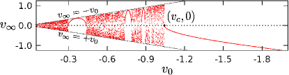
In the first simulation we use a $v_{0}$-interval starting at a relatively low velocity ($>-0.05$) and ending at very large velocity ($<-5.0$). We verified that for large values of $|v_{0}|$ the collision is elastic and consists of only one interaction with the solitons passing through each other. At lower velocities there is a critical point $(v_{c},0)$, such that as $v_{0}$ approximates the critical velocity $v_{c}\approx-1.04$ the collision becomes each time more inelastic. If $v_{0}>v_{c}$ (i.e, $|v_{0}|<|v_{c}|$) the dynamics of the interaction changes completely and the solitons collide in an unpredictable fashion. This is shown in Fig. 1 for the exit velocity limited to the range $[-0.05,-2.00]$. The irregular scattering of the solitons is characterized by the high sensitivity of the initial condition, i.e., the collisional velocity $v_{0}$. Note that all points in the plot are contained in a cone of maximum exit velocity, which is given by the dotted-lines ($v_{\infty}=\pm v_{0}$), which means that in the current configuration of our system the inequality $|v_{\infty}|\leq|v_{0}|$ holds, and the solitons can not gain momentum through symmetric collisions.

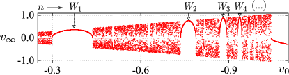
The region $v_{0}>v_{c}$ is shown in more details in Fig. 2 (top), where we detect the existence of several windows of lump-like shape that repeats indefinitely as $v_{0}$ tends to $v_{c}$. In these windows the soliton scattering is not sensitive to $v_{0}$, in fact, we verified that inside each window the collision resembles a reflection process, with the solitons forming a bound-state with fixed lifetime ($z$-interval of existence of the bound-state) and escaping toward the same region ($T>0$ or $T<0$), i.e., its initial position. This type of window is called reflection window. An interesting feature of the reflection window is that for any value of the initial velocity within it, the soliton profile oscillates the same number of times, in which one shape-oscillation was taken to be one period of oscillation of the width of the solitons. This last statement leads to the property of a fixed lifetime of the bound-state of the solitons, as mentioned before. Also, the differences between the lifetimes of bound-states of any two successive windows are always one shape-oscillation period. We designate these windows by $W_{n}$, as seen in Fig. 2 (top), with $n$ being the window index. The numbering starts with the largest window ($n=1$). Also, in Fig. 2 (bottom) the details of the collisions are shown for values of $v_{0}$ within four successive reflection windows, the number of shape-oscillations ($N_{SO}^{n}$) was found to be related to $n$ by $N_{SO}^{n}=n+3$. The value of $N_{SO}^{n}$ is obtained by counting the number of amplitude peaks in the soliton, which is easily seen in the contour plots. We noticed that these windows form a structure, which consist of a repetition of windows separated by intervals that become smaller as $v_{0}$ approaches $v_{c}$. The window shape is basically a lump with the crest almost tangent to the cone of maximum $v_{\infty}$, it becomes narrower as closer it is from the critical point.

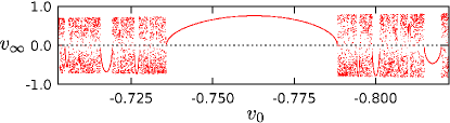
In Fig. 2 we noticed the existence of some smaller window structures in the edges of each reflection window. Then, to provide a better visualization of it we simulated in an interval centered at $W_{2}$, where the resultant exit velocity graph is shown in Fig. 3. In this figure two structures appear clearly, one resembling a mirrored image of the other. Besides, both are very similar to the one in Fig. 2, but with the windows being like valleys instead of lumps. These are called transmission windows because the collisions associated to it resemble a transmission process. As seen in the first exit velocity graph, the windows become narrower and closer spaced near the critical points. For the structures in Fig. 3 these points are located in the edges of the reflection window $W_{2}$.

Figure 3: (Color online) Result for the simulation in an interval centered at $W_{2}$ (Fig. 2 (top)). The size of the interval was chosen to totally encompass the window structures that appear in the edges of the reflection window $W_{2}$.

Figure 4: (Color online) Results of successive amplifications of slim $v_{0}$-intervals between certain reflection and transmissional windows as marked in figures: (a) top part of Fig. 2 that is used to emphasize the pattern repetition; (b)-(e) are successive amplifications of the intervals marked in the exit velocity graphs, where we verify similar window structures to those ones appearing in (a).

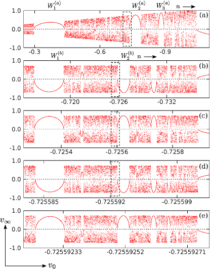
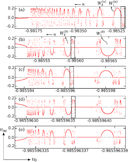
To explore the smaller structures embedded in the region $|v_{0}|<|v_{c}|$ we performed simulations amplifying the structures located in narrower $v_{0}$-intervals near the edges of certain windows. Firstly, we chose the left edge of the window $W_{2}$, which yielded a structure of windows similar to the ones seen until now. Hence, we expected that smaller structures with same pattern could be found by applying the same procedure. So, we have adopted a protocol that consists of choosing intervals for amplifications always in the left edge of every second window of any structure that may appear in the successive amplifications. Following this protocol we obtained the results shown in Fig. 4, where the first plot is the same of Fig. 2 (top). The highlighted intervals in the plots indicate the region of amplification, which corresponds to the plot immediately bellow. Here we modified our notation for labeling reflectional/transmissional windows, such that the superscript $(s)$ were added to denote the structure in which the window is located, i.e., $W_{n}^{(s)}$ is the label of the $n$-th window in the structure in Fig. 4(s), with $s=a,b,...,e$. We extend this notation to the critical velocity associated with each structure, here denoted by $v_{c}^{(s)}$.

We observed that for all scattering data obtained, zero exit velocities have appeared only for collisions associated with initial velocities between zero and the window $W_{1}^{(a)}$. In order to verify the true outcome of these collisions, very long simulations were performed. We found that the bound-state formed during the collision eventually ends for a certain $z$ much larger than $z_{max}$. Thus there are only two different scenarios concerning the solitons’ collisions accordingly to the reduced ODE model, namely, transmissional collision ($v_{\infty}<0$) and reflectional collision ($v_{\infty}>0$). Our simulations show that transmission and reflection windows are distributed along very slim intervals within the chaotic region ($|v_{0}|<|v_{c}|$), where the collision dynamic is indeed very sensitive to the choice of $v_{0}$. The most interesting feature found for the exit velocities are the structures that repeat embedded in itself, forming in the edges of every window, as shown before in Fig. 3. Besides, they have a very similar pattern regarding the size and distribution of the windows. It is clearly seem that Fig. 4(a) resembles Figs. 4(c) and 4(e), also the Fig. 4(b) resembles Fig. 4(d). This suggests that the structures always appear alternating the window type. Also, excepting in Fig. 4(a), they seem to be related by just one symmetry operation, i.e., a reflection about the $v_{0}$-axis.

By analyzing the window patterns for the structures in Fig. 4, we found that the velocity $v_{n}^{(s)}$ in the crest (trough) of a reflection (transmission) window $W_{n}^{(s)}$ and the critical velocity $v_{c}^{(s)}$ of the structure given in 4$(s)$ are very well related by Yang (2010); Tan and Yang (2001)

$$\dfrac{1}{\sqrt{|(v_{c}^{(s)})^{2}-(v_{n}^{(s)})^{2}|}}=p^{(s)}n+q^{(s)}\,,$$ (10)

where the coefficients $p^{(s)}$ and $q^{(s)}$ vary for the different values of $s$. We illustrate this fact for the windows until index $n=6$, the linear relation in (10) is satisfied with great precision for the Fig. 4(a), while for the other structures in Figs. 4(b)-(e) we found relative small standard deviations. These results allowed us to infer that the window patterns in the intervals of our simulations satisfy a common relation given by (10), however, it is not enough to conclude that the pattern is closely the same, since the coefficients can not be compared because the structures have different sizes. We solved this problem by rescaling and displacing the structures, in a manner that the left edge of $W_{1}^{(s)}$ is at the origin and the critical point of every structure at $(-1,0)$. This transformation changes the values of the initial velocities in the crest (trough), which are denoted by $\widetilde{v}_{n}^{\,(s)}$. In this way we can say that $\widetilde{v}_{c}^{\,(s)}\equiv-1$ for all $(s)$, with $\widetilde{v}_{n}^{\,(s)}<\widetilde{v}_{c}^{\,(s)}$. So, the transformed structures have the same size. The coefficients found for the first structure are $\widetilde{p}^{\,(a)}=0.325\pm 0.006\,(1.85\%)$ and $\widetilde{q}^{\,(a)}=0.65\pm 0.02\,(3.08\%)$, while for the remaining structures we calculated the average of the coefficients together with the standard deviations $\langle\widetilde{p}\rangle=0.280\pm 0.003\,(1.24\%)$ and $\langle\widetilde{q}\rangle=0.662\pm 0.004\,(0.68\%)$. Note that these averages values have very small standard deviations, but there is a relevant difference when comparing $\langle\widetilde{p}\rangle$ and $\widetilde{p}^{\,(a)}$. These results show that the window pattern is almost the same for all structures after the first amplification. We stress that the first exit velocity plot presents a subtle difference among the others, which resides in the region where zero exit velocities appeared (which is purely chaotic), differently from the other structures. Hence a self-similarity argument can be applied only to Figs. 4(b)-(e).

In Fig. 5 we show the quantity $[1-(\widetilde{v}_{n}^{\,(s)})^{2}]^{-1/2}$ as a function of the window index $n$. Note that the curves related to the structure presented in Figs. 4(c)-(e) are too close to be distinguished and the curve related to Figs. 4(b) is also very close from those. Also, our observations indicate that this pattern prevails for any window structure embedded into the Fig. 4(a), which is a characteristic feature of a fractal pattern and demonstrate the chaotic behavior of the scattering. Furthermore, we verify that the size ($L^{(s)}$) of the window structure in Fig. 4(s), which is the length between the left edge of the first window and the critical velocity $v_{c}^{(s)}$, nicely satisfies the formula

$$\log_{10}L^{(s)}=Rj+r\,,$$ (11)

where $j=1$ for Fig. 4(a), $j=2$ for Fig. 4(b), and so on. Moreover, the integer number $j-1$ is the number of amplifications. In Eq. (11) the linear fit yielded $R=-1.639\pm 0.008\,(0.47\%)$ and $r=1.56\pm 0.02\,(1.63\%)$. After some algebra, the length $L^{(s)}$ can be expressed in terms of the $j$ and $L^{(a)}$ as

$$L^{(s)}=10^{R(j-1)}L^{(a)}\,.$$ (12)

Since $R$ is a negative constant, the factor that multiplies $L^{(a)}$ in (12) is less than unity and we call it as reduction factor. Note that this results implies that length of the window structures decreases exponentially with the number of amplifications. Therefore the zoom ratio is closely the same at each amplification, which is given by $10^{-R}\approx 43.6$ (the reduction ratio is the inverse). As an example, to emphasize how is this reduction, for structure in Fig. 4(e) ($j=5$) one obtains the reduction factor $\sim 10^{-7}$, while for structure in Fig. 4(d) ($j=4$) it is $\sim 10^{-2}$.

Figure 5: (Color online) Plot of $[1-(\widetilde{v}_{n}^{\,(s)})^{2}]^{-1/2}$ as a function of the the window index $n$. In curves (a)-(e) we used data obtained by the structures shown in Fig. 4(a)-(e), respectively.

Figure 6: Profile of the localized solution $|\psi(z,T)|^{2}$ during the interaction with the field $|\phi(z,T)|^{2}$ obtained using the reduced ODE model of Eqs. (1a) and (1b). The initial velocity values are taken within four successive windows in the structure shown in Fig. 4(s), with $s=\{b,c,d,e\}$. The number of shape-oscillations in the bound-state of the solitons yields $N_{SO}^{n}=(n-1)+m^{(s)}\times 4+4$ for any $W_{n}^{(s)}$ window (including Fig. 2(botton)), in which the integer $m^{(s)}$ was introduced to designate the number of amplifications ($m^{(s)}=j-1$), with $m^{(a)}=0$, $m^{(b)}=1$, etc.

In Fig. 6 we show details of the collisions for the transmission windows in Figs. 4(b) and (d) and for the reflection windows in Figs. 4(c) and (e). Again, we note the formation of a bound-state with fixed lifetime for any value of $v_{0}$ within the same window, and also, collisions of successive windows differs only by one shape-oscillation period. Thus, the interesting feature observed for the reflection windows in the first structure extends for any window, where the collision may be of type transmission or reflection.

The self-similarity involving the structures in Fig. 4 and the high sensitivity to the initial conditions, reinforce the hypothesis that the soliton scattering described by the reduced ODE model is chaotic and the exit velocity plots are different views of a fractal. Thus, we found that the reflection and transmission windows are intervals where the chaotic behavior disappears, that is, for any $v_{0}$ taken within these windows one can immediately predict the outcome of the collision, as well as the lifetime of the solitons bound-state.

III.2 Direct numerical simulations

The coupled NLS equations (1a) and (1b) were simulated by using the split-step method to perform the temporal evolution of the fields. To solve the linear part of the equations we used the Crank-Nicholson algorithm while for the nonlinear part we applied the $4^{\text{th}}$-order Runge-Kutta algorithm. Also, we take the initial conditions for simulations of solitons’ collisions in the form

$$\psi(0,T) =\exp\left\{\frac{1}{2}\left(1+\frac{1}{g}\right)+g(T-T_{0})^{2}+\frac{i}{4}v_{0}T\right\},$$ (13a)

$$\phi(0,T) =\exp\left\{\frac{1}{2}\left(1+\frac{1}{g}\right)+g(T+T_{0})^{2}-\frac{i}{4}v_{0}T\right\},$$ (13b)

where the initial separation $2T_{0}$ needs to be large enough to provide a negligible overlap of the solitons tails at $T=0$, such that the localized solutions are indeed a good approximation for the fields at $z=0$. In our case it was taken to be equal to $20$ dimensionless units. As mentioned before, localized solutions are obtained for negative values of $g$ in the nonlinear term (in our case we set $g=-1$). In the collision simulations, the spatial interval were [$-50,50$], the $T$-stepsize were $0.04$, and the $z$-stepsize $0.001$, values that satisfy the CFL condition associated with the implemented discretization in the linear part of the coupled NLS equations given by Eqs. (1a) and (1b). We verified that for wider spatial intervals there will be no significant changes for the collision results in the observed bound-state scenarios. The numeric procedure was implemented with the same numerical precisions used in the variational approach. In our simulations, we found to be negligible the losses by radiation due to the approximate solution profile used as initial conditions. In order to avoid very long simulations, we analyze the position of both solitons to predict whether the collision leads to a trapping scenario or not, and if so we assign a null value to the exit velocity. Several simulations were performed to investigate the scattering of solitons under the same conditions addressed in the reduced ODE model. The parameter $v_{0}$ was varied in intervals with $5000$ grid points, where these intervals were chosen in accordance with the results obtained in the variational model.

The obtained scattering data shows that three collision scenarios are possible, viz., transmission, reflection, and trapping ones. We stress that trapped solitons were not observed in the reduced ODE model, which was expected because no radiation emission process is described by that model Yang and Tan (2000); Tan and Yang (2001); Yang (2010).

The first exit velocity graph acquired from the direct numerical simulations is shown in Fig. 7, where one can note the existence of a critical velocity $v_{c}\approx-0.993$ that separates the region of chaotic scattering from the region of regular scattering. Similarly to the reduced ODE model, the critical velocity is very close to $-1$ and the collision is elastic only if $v_{0}\ll v_{c}$ ($|v_{0}|\gg|v_{c}|$). This first view of the exit velocity graph reveals the existence of reflection and transmission windows with different shapes, where some of these windows appear distributed uniformly only in a tiny interval limited by the critical velocity at the right side and the edge of a transmission window at the left side, which is indicated with an arrow in Fig. 7 and shown amplified in Fig. 8(a). By analyzing the windows structure revealed by the collisional dynamics in Fig. 8(a), we found the same feature of the reduced ODE model, that is, the outcome of each collision with initial velocity within a specific window is always of reflective type, preceded by a bound-state of same lifetime and number of shape oscillations. Note that this first amplification yields a windows structure that resembles the first one provided by the reduced ODE model (Fig. (4)(a)). However, in the numerical simulations we observe a great number of trapped states, returning null output velocities. Also, we noted a small difference in the width and position of the windows when comparing both models.

The second amplification was taken in the right edge of the largest window of Fig. 8(a), which is highlighted by a dashed rectangle, corresponding to the plot displayed in Fig. 8(b). To construct the plots of each amplification we performed new simulations for $5000$ different values of input velocities $v_{0}$ within the appropriate range. Furthermore, Fig. 8(b) revealed a structure composed by transmission windows with different spacing. Indeed, one can note that this structure is more similar to those obtained by reduced ODE model than the previous structure. From this point, we proceeded with amplifications following a protocol equivalent to that employed in the reduced ODE model simulations. This region allow us to get a symmetry for each amplification, changing only by a reflection in vertical axis, which simplifies our analysis of the fractal pattern. Note that the Fig. 8(c) appears approximately as a reflection of Fig. 8(b). We observe this pattern when comparing Figs. 8(c) and 8(d), as well as Figs. 8(d) and 8(e). In addition, we get very similar patterns revealing a fractal structure when comparing the amplifications shown in Figs. 8(b) and 8(d) and Figs. 8(b) and 8(d). As we observed in the reduced ODE model, the bound-state associated with two successive windows in structures of Figs. 8(a)-(e) differs only by one shape-oscillation, which can be expressed by $N_{SO}^{n+1}=N_{SO}^{n}+1$. Using the same notation $W_{n}^{(s)}$, we highlighted the first two windows in the Figs. 8(a) and 8(b), indicating the sequence used for the index $n$. In Fig. 9 we display some examples of collision scenarios obtained via direct numerical simulations with values of initial velocities within four successive windows in each structure shown in Figs. 8(a)-(e).

Figure 7: (Color online) Exit-velocity $v_{\infty}$ versus collision-velocity $v_{0}$ obtained via direct numerical simulations of Eqs. (1a) and (1b) with initial conditions given by Eqs. (13a) and (13b). The arrow indicates the critical velocity $v_{c}$, above which (in absolute value) no longer obtains the chaotic pattern.

Figure 8: (Color online) Successive amplifications of exit-velocities ($v_{\infty}$) versus input-velocities ($v_{0}$) due to the scattering of solitons. (a) Result of the amplification of the tiny interval close to the arrow (left side) in Fig. 7; (b)-(e) are successive amplifications of the intervals highlighted in the exit-velocity graphs (a)-(d), respectively.

Figure 9: Profile of the localized solution $|\psi(z,T)|^{2}$ during the interaction with the field $|\phi(z,T)|^{2}$ obtained via direct numerical simulations of Eqs. (1a) and (1b). The initial velocity values are taken within four successive windows in the structure shown in Fig. 8(s), with $s=\{a,b,c,d,e\}$. By counting the number of shape-oscillations in the solitons bound-state we found $N_{SO}^{n}=(n-1)+m^{(s)}\times 4+13+N_{0}$ (where $N_{0}=1\Longleftrightarrow m^{(s)}=0$, otherwise $N_{0}=0$) for any $W_{n}^{(s)}$ window.

A similar analysis, previously realized for the window patterns in the reduced ODE model, was performed here considering the structures in Fig. 8. The relation involving the quantities $[|(v_{n}^{(s)})^{2}-(v_{c}^{(s)})^{2}|]^{-1/2}$ and the window index $n$ is also very well established in accordance with Eq. (10), hence the slope $\widetilde{p}^{\,(s)}$ and the intercept coefficient $\widetilde{q}^{\,(s)}$ were obtained for the structures transformed in the same way described before. We found $\widetilde{p}^{\,(a)}=0.047\pm 0.002\,(4.26\%)$ and $\widetilde{q}^{\,(a)}=0.941\pm 0.009\,(0.96\%)$. Again, for the remaining rescaled structures, we calculated the average of the coefficients together with their standard deviations, yielding $\langle\widetilde{p}\rangle=0.271\pm 0.006\,(2.23\%)$ and $\langle\widetilde{q}\rangle=0.667\pm 0.006\,(0.84\%)$. Clearly, these values present relevant differences when compared with $\widetilde{p}^{\,(a)}$ and $\widetilde{q}^{\,(a)}$, respectively. Therefore, these results provide a numerical evidence that the window spacing of the structure in Fig. 8(a) and the amplified ones embedded in it are indeed very different when compared. Also, since $\widetilde{p}^{\,(a)}<\langle\widetilde{p}\rangle$, the window pattern of the Fig. 8(a) contain less spaced windows, as one can see in the plots. In Fig. 10 is displayed the relation between $[1-(\widetilde{v}_{n}^{\,(s)})^{2}]^{-1/2}$ and the window index $n$. The remarkably linear relation of these quantities appears very well established as well as in the result obtained with the reduced ODE model. Additionally, comparison between the values of $\langle\widetilde{p}\rangle$ yielded by the direct and variational approach shows that they differ only by $\sim 3.2\%$. This reinforces that the reduced ODE model provides a very good approximation regarding the window pattern. Since the linear relation in Eq. (10) it is suitable for the window spacing description, it can be used as an estimative of the position of very narrow windows that are difficult to access.

Figure 10: (Color online) Plot of $[1-(\widetilde{v}_{n}^{\,(s)})^{2}]^{-1/2}$ as a function of the the window index $n$. In (a)-(e) we used data obtained by the structures shown in Fig. 8(a)-(e), respectively.

When analyzing the length of the structures given by the direct numerical simulations, we found that all structures resultant of amplifications obey with great precision the linear relation given by Eq. (11), for which the coefficients are $R=-1.481\pm 0.006\,(0.43\%)$ and $r=-0.91\pm 0.02\,(2.34\%)$. As shown in Eq. (12), only the coefficient $R$ is important in the zoom ratio. By comparing its value provided by the two approaches we found a difference of $\sim 9.6\%$. However, the first window structure of the direct numerical simulations has a length that is more than two orders of magnitude smaller than the length found in the variational approach, resulting in even smaller structures when amplifying.

III.3 Analysis of soliton scattering for both approaches

Figure 11: Scheme identifying the initial bound state and the final bound-state, the collisions in the figure are plotted as contour lines of $|\psi(z,T)|^{2}$, the initial velocity was taken in the $W_{4}^{(e)}$ window for structures in Fig. 4(e) (top) and Fig. 8(e) (bottom). In these collisions the fifth passing (P5) is when the bound-state changes. At the left side of the figure we highlight how the final bound-state depends upon $n$, the symbols $\uparrow$, $\downarrow$ and $\circ$ indicate whether energy of the mode has increased, decreased or kept unchanged, respectively.

In order to compare the soliton collision dynamics given by the two employed methods, we analyze only the interaction stage that follows after the waves cross the $z$ axis at $T=0$, where they overlap at most and energy can be exchanged between the solitons and their internal and external modes. A mechanism of resonance energy exchange between the internal and translational modes of the solitons was proposed in Ref. Campbell et al. (1983), where this mechanism was employed to describe a structure of reflection windows intertwined by trapping intervals in kink-antikink collisions. The energy exchange was found to take place at the instants of great overlap of the waves, which is when an internal mode can become active by storing part of the kinetic energy. The resonance mechanism was associated to the existence of fractal window structure resultant in kink-antikink collisions in the scalar $\lambda(\phi^{2}-1)^{2}$ theory Anninos et al. (1991), and in Refs. Yang (2010); Yang and Tan (2000); Tan and Yang (2001) regarding vector-soliton collision. Here we also adopt this mechanism to explain how the soliton exchange kinetic energy with its oscillation-mode, which store energy in soliton’s shape vibrations. In our simulations we noted that this exchange also occurs when the solitons overlap at most by passing each other.

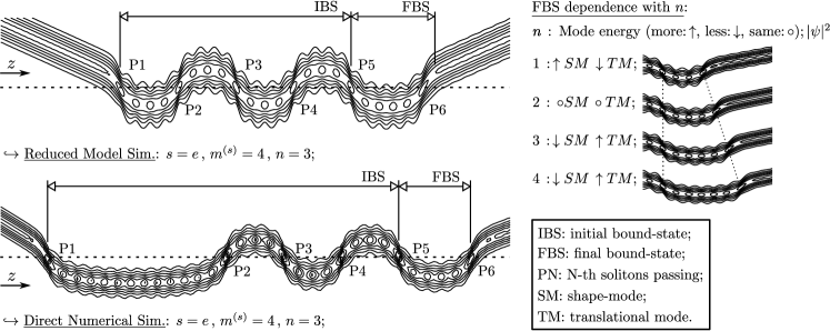
For our system, the analysis of the exit velocity plots presented previously revealed how sensitive can the collision dynamic be. Indeed, just after the solitons pass each other for the first time, what follows next depends on the impact velocity that is directly related to $v_{0}$. Considering the controlled collision scenarios provided by reflection/transmission windows, in the first passing drained kinetic energy sets up shape-oscillations, then the attraction interaction binds the solitons that remain in a bound-state until they bounce (moving forth and back) to pass each other again. How the energy is exchanged again depends greatly of the relative phases of the internal modes of the solitons, as discussed in Ref. Anninos et al. (1991). If enough kinetic energy is restored the pair unbinds, otherwise the bound-state prevails. In Figs. 6(a)-(d) and 9(b)-(e) the bound-state dynamics are initially the same for every window in a given structure, considering the bouncing motion and the number of shape-oscillations, but it changes in a different manner at a certain passing. In both approaches we verified that these changes happen when the solitons pass each other $(m^{(s)}+1)$ times and after that another type of bound-state arises. This final bound-state precede the unbinding of the solitons and has a varying dynamics, in which the translational mode can lose energy ($n=1$), keep it unchanged ($n=2$) or increase it ($n>2$). In any figure regarding these collisions one can realize what changed in the solitons kinetic energy by looking at the number of shape-oscillation during a complete bounce of the solitons. If it was shortened, for example, then more energy was drained from the translational mode.

In the direct numerical simulations the initial bound-state has a longer lifetime and the solitons bounce around the $z$-axis as in variational approach, but before the second passing time the bound-state has less energy in the internal modes and more energy in the translational modes, resulting in a longer bouncing motion as seen in the Figs. 9(b)-(e). The dynamic of this bound-state initially resembles the collision for the first window in Fig. 9(a), which presents the same number of shape-oscillations. Therefore, the final bound-state dynamics depends upon $n$, furthermore it changes in the same manner of the single bound-states formed in the first structure of windows (in which there is only the final bound-state). This last statement is valid for both presented approaches. In Fig. 11 we show a scheme that identify the initial and final bound-state that appear in a reflectional collision, which is associated to the $W_{4}^{(e)}$ window found after the fourth amplification. We highlight in this figure how the final bound-state depends upon $n$, and also whether the internal or translational modes acquire energy after the exchange.

Hitherto we have omitted the losses by radiation, which have an important role in the solitons’ collision dynamics. These losses can be excited during the instants of energy exchange and carry out energy of the translation and/or internal modes of the solitons. In Ref. Anninos et al. (1991) the energy taken by the radiation losses is later retransferred to the pair, while for vector-soliton collisions they develop a different role in the dynamics. As mentioned before, although the variational approach describe very well the resonance mechanism involving the translational and internal modes, it does not support radiation losses due to the constraints imposed by the ansatz. This explains the absence of trapping scenarios in our simulations of the reduced ODE model, since radiation emission can prevent the translational modes to recover enough energy to unbind the bound-state of solitons, which does happen in the direct numerical simulations of the field equations. In these simulations, all the trapping scenarios are characterized by the solitons quickly bouncing around the $z$-axis while very close to each other. In contrast, for a collision described by the reduced ODE model we attested that after a sufficiently long time eventually occurs a phase matching of internal modes, retransferring kinetic energy to the solitons, in a such way that they can immediately unbind or bounce until a final energy exchange that results in a definitive unbinding.

Since there is no radiation emission in the reduced ODE model, solitons are able to escape with velocity $|v_{\infty}|\leq|v_{0}|$ in the variational description, and the height (depth) of the reflection (transmission) windows is closely equal to the value $|v_{0}|$ corresponding to the its maximum (minimum). On the other hand, in the direct numerical simulations radiation emission always happens during the bound-state, which results in $|v_{\infty}|$ always smaller than $|v_{0}|$ in all structures. When solitons unbind and move away, the exit velocity value show us if the internal modes remained excited after the collision because the smaller the value of $|v_{\infty}|$ is, compared with $|v_{0}|$, greater is the energy in shape oscillation. Analyzing the radiation emitted during the collisions in the direct numerical simulations, we noted that it happens not only when the solitons pass through each other, but also when they are moving side by side as a bound-state. This means that such radiation losses play an important role in the window structure and in the dynamics of the reflectional/transmissional collisions, and not only in trapping scenarios.

By a graphical analyses of the solitons’ collisions, we found that its lifetime ($Z_{n}^{(s)}$) is nicely predicted by a multi-linear function of the integer quantities $n$ and $m^{(s)}$, likewise the number of shape-oscillations $N_{SO}^{n}$, as shown in Figs. 6 and 9. They are given by

$$Z_{n}^{(s)} = (n-1)z_{f}+m^{(s)}z_{i}+z_{1}\,;$$

$$N_{SO}^{n} = (n-1)+4m^{(s)}+4\,;$$ (14)

$$\hookrightarrow \begin{cases}z_{f}&=2.39\pm 0.02\,(0.65\%)\\ z_{i}&=10.16\pm 0.06\,(0.57\%)\\ z_{1}&=7.9\pm 0.1\,(1.26\%),\end{cases}$$

for the variational model simulations, and

$$Z_{n}^{(s)} = (n-1)z_{f}+m^{(s)}z_{i}+z_{1}\,;$$

$$N_{SO}^{n} = (n-1)+4m^{(s)}+13+N_{0}\,,$$ (15)

(where $$N_{0}=1\Longleftrightarrow m^{(s)}=0 N_{0}=0$$, otherwise ) ;

$$\hookrightarrow \begin{cases}z_{f}&=2.38\pm 0.07\,(3.01\%)\\ z_{i}&=9.4\pm 0.4\,(4.61\%)\\ z_{1}&=31.5\pm 0.9\,(2.79\%),\end{cases}$$

for the direct numerical simulations. We point out that in (15) the relation for $N_{SO}^{n}$ is multi-linear only for the amplified structures ($m^{(s)}>0$), which is due to $N_{0}$ that was added to encompass all the structures in a single formula. In (14) and (15), $z_{f}$ and $z_{i}$ are characteristic times of the final bound-state (FBS) and initial bound-state (IBS) (see Fig. (11)), respectively, while $z_{1}$ is the lifetime of the bound-state associated with the first reflection window of the first window structure (given by $n=1$ and $m^{(a)}=0$ in both formulas). The coefficient $z_{f}$ represents the width $\Delta z$ of the solitons’ shape vibration in the FBS. The results show that it is closely the same for every structure, which means that the quantity of energy stored in the internal mode influences only in the amplitude of the shape vibrations and not in its frequency. The $z_{i}$ coefficient represents the width $\Delta z$ of the solitons bounce (shortest bounce in the direct numerical simulations) in the IBS. The multi-linear relations for $Z_{n}^{(s)}$ and $N_{SO}^{n}$ are clearly similar, but this is an expected result since each coefficient in $Z_{n}^{(s)}$ is related to a number of shape-oscillations. For the reduced ODE model, both $Z_{n}^{(s)}$ and $N_{SO}^{n}$ can be well predicted for the bound-states by using the formulas above, while for the direct numerical simulations they provide a less precise prediction for $Z_{n}^{(s)}$, but still reasonable. The numerical values of the coefficients in these formulas give us some useful information about the two approaches. The difference between the $z_{1}$ coefficients reproduces the difference seen in the first bounce in the IBS, which resides mainly in the number of shape-oscillations that is provided by the last coefficient of the $N_{SO}^{n}$ formulas, where for the variational approach it is $4$ and for the direct numerical simulations it is $14$. The other $z$-coefficients have similar values. Additionally, the FBS lifetime and shape vibrations are nicely reproduced by the reduced ODE model.

IV Conclusion

In conclusion, we studied the fractal scattering of Gaussian solitons in directional couplers with logarithmic nonlinearities. In this sense, we employed two methods, viz., the variational approach and direct numerical simulations. Regarding the variational approach, we have started our study by firstly developing the reduced ODE model for our system governed by the field equations (1a) and (1b), which provided the results presented in the section II. The reduced ODE model description shows that the collisions of the solitons is chaotic when the absolute value of the input velocity is less than a certain critical value, and a fractal structure composed by reflection and transmission windows arises within the chaotic region. In the same way, in view to verify the feasibility of the reduced ODE model in the present context we performed direct numerical simulations. So, in Sec. III we shown similar features presented by the two approaches employed.

Our analysis on the size of the structures and window positions yielded quite precise results for the fitting curves. As long as the amplifications follow the adopted protocol these structures closely preserve their window pattern and they are all embedded in each other in a quite well defined manner, which means that the amplifications almost occur in the same ratio. Interestingly, a numerical comparison of the window pattern and amplification ratio of both variational and direct numerical approaches shows that these are not very much different. Once again, it reinforces the usefulness of the variational model in predicting the major features of solitons scattering and collision dynamics.

This study also gives us an idea about the form of collisions of solitons in reflection/transmission windows within the chaotic region, which can enable us to control the pattern of collision via initial approach velocity between them. Also, due to sensitivity to small changes in the velocity, we theorize that it could be used as a kind of sensor to verify inhomogeneities caused by impurities in the medium. In this sense, we are studying other models as well as including tests of effects of inhomogeneities in the medium.