Abstract

In this paper we study inexact dumped Newton method implemented in a distributed environment. We start with an original DiSCO algorithm [Communication-Efficient Distributed Optimization of Self-Concordant Empirical Loss, Yuchen Zhang and Lin Xiao, 2015]. We will show that this algorithm may not scale well and propose an algorithmic modifications which will lead to less communications, better load-balancing and more efficient computation. We perform numerical experiments with an regularized empirical loss minimization instance described by a 273GB dataset.

1 Introduction

As the size of the datasets becomes larger and larger, distributed optimization methods for machine learning have become increasingly important Bertsekas & Tsitsiklis (1989); Dekel et al. (2012); Shamir & Srebro (2014). Existing mehods often require a large amount of communication between computing nodes Yang (2013); Jaggi et al. (2014); Ma et al. (2015b); Yang et al. (2013), which is typically several magnitudes slower than reading data from their own memory Marecek et al. (2014). Thus, distributed machine learning suffers from the communication bottleneck on real world applications.

In this paper we focus on the regularized empirical risk minimization problem. Suppose we have $n$ data samples $\{x_{i},y_{i}\}_{i=1}^{n}$, where each $x_{i}\in\mathbb{R}^{d}$ (i.e. we have $d$ features), $y_{i}\in\mathbb{R}$. We will denote by $X$ the data matrix, i.e. $X:=[x_{1},...,x_{n}]\in\mathbb{R}^{d\times n}$. The optimization problem is to minimize the regularized empirical loss

$$f(w):=\frac{1}{n}\sum_{i=1}^{n}\phi_{i}(w,x_{i})+\frac{\lambda}{2}\|w\|_{2}^{2},$$ (P)

where the first part is the data fitting term, $\phi:\mathbb{R}^{d}\times\mathbb{R}^{d}\rightarrow\mathbb{R}$ is L-smooth loss function which typically depends on $y_{i}$. The second part of objective function (P) is $\ell_{2}$ regularizer ($\lambda>0$) which helps to prevent over-fitting of the data.

There has been an enormous interest in large-scale machine learning problems and many parallel Bradley et al. (2011); Recht et al. (2011) or distributed algorithms have been proposed Agarwal & Duchi (2011); Takáč et al. (2015); Richtárik & Takáč (2013); Shamir et al. (2013); Lee & Roth (2015).

From algorithmic point of view some researches try to minimize (P) directly including SGD Shalev-Shwartz et al. (2011), SVRG and S2GD Johnson & Zhang (2013); Nitanda (2014); Konečný et al. (2014) and SAG/SAGA Schmidt et al. (2013); Defazio et al. (2014); Roux et al. (2012). On the other side, one very popular approach is to solve its dual formulation Hsieh et al. (2008) which has been successfully done in multicore or distributed settings Takáč et al. (2013); Jaggi et al. (2014); Ma et al. (2015b); Takáč et al. (2015); Qu et al. (2015); Csiba et al. (2015); Zhang & Xiao (2015). The dual problem of (P) has following form:

$$\max_{\alpha\in\mathbb{R}^{n}}D(\alpha):=-\frac{1}{n}\sum_{i=1}^{n}\phi^{*}_{i}(-\alpha_{i})-\frac{\lambda}{2}\|\frac{1}{\lambda n}X\alpha\|^{2},$$ (D)

$\phi_{i}^{*}$ is a convex conjugate function of $\phi_{i}$.

The Challenge In Distributed Computing.

We can identify few challenges when we deal with high-performance distributed environment.

1. Load-Balancing. Assume that we have $m$ computational nodes available use. In order to have an algorithm, which is scalable, the algorithm should make each node equally busy. Amdahl’s law Rodgers (1985) implies that if the parallel/distributed algorithm runs e.g. 75% of the time only on one of the nodes (usually the master node), then the possible speed-up of the algorithm is bounded by $\frac{1}{0.75+0.25/m}$ and is shown on Figure 1 and is asymptotically bounded by $4/3\approx 1.333$.

   Hence, any algorithm which is targeted for a very large scale problems has to be design in such a way, that the sequential portion of the algorithm is negligible.

   

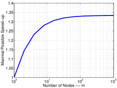
   Figure 1: Maximal possible speed-up of an Algorithm which runs 75% in sequential mode.

2. Communication efficiency. As it was stressed in the introduction, in a distributed setting the communication between nodes should be avoided or minimized (if possible). Another challenge is to balance the time the nodes are going some computation and the time they spent in the communication (usually in MPI calls).

In this paper we modify the design of promising DiSCO algorithm Zhang & Xiao (2015). We completely redesign the algorithm (partitioning of the data, preconditioning, communication patterns) to get a new algorithm which

1. has very good scaling (the serial computation is almost negligible),

2. balances work-load equally between nodes (all the nodes are working all the time, no real job for master node),

3. has much smaller amount of data set over the network than in the original DiSCO algorithm.

1.1 Related Work

As stressed in the previous section, one of the main bottlenecks in distributed computing is communication. This challenge was handled by many researchers differently. In the ideal case, one would like to never communicate or maybe communicate only once at the end to form a result. However, such a procedure which could communicate only max once and would be able to give arbitrary good solutions (when no node can have access to all the data) is more fantasy than reality.

Hence, to somehow ”synchronize” work on different computing nodes, researchers use various standard technique from optimization. Few of them based their algorithms on ADMM type methods Boyd et al. (2011); Deng & Yin (2012), another used block-coordinate type algorithms Lee & Roth (2015); Yang (2013); Jaggi et al. (2014); Ma et al. (2015b), where they solved on each node some local sub-problems which together formed an upper-bound on the optimization problem. The balancing of computation and communication was achieved by varying the accuracy of the solutions of the local sub-problems, which turns out to be more efficient than some earlier approaches Takáč et al. (2013; 2015)).

Let us now give an overview of existing approaches to solve problem (P) in distributed setting:

1. SGD-based Algorithms. For the empirical loss minimization problems of interest here, stochastic subgradient descent (SGD) based methods are well-established. Several distributed variants of SGD have been proposed, many of which build on the idea of a parameter server Niu et al. (2011); Liu et al. (2014); Duchi et al. (2013). The downside of this approach, even when carefully implemented, is that the amount of required communication is equal to the amount of data read locally (e.g., mini-batch SGD with a batch size of 1 per worker). These variants are in practice not competitive with the Newton-type methods considered here, which allow more local updates per communication round.

2. ADMM. An alternative approach to distributed optimization is to use the alternating direction method of multipliers (ADMM), as used for distributed SVM training in, e.g., Forero et al. (2010). This uses a penalty parameter balancing between the equality constraint and the optimization objective Boyd et al. (2011). However, the known convergence rates for ADMM are weaker than the more problem-tailored methods mentioned previously, and the choice of the penalty parameter is often unclear.

3. DANE Algorithm.

   The DANE (Distributed Approximate Newton) algorithm Shamir et al. (2013) is applicable to solve problems (P) with any smooth loss functions, which genreally requires two rounds of communication in each iteration. In $k$-th iteration, the first round of communication is used to compute the gradient $f^{\prime}(w_{k})$ by a ReduceAll operation on a $\mathbb{R}^{d}$ vector. Then each machine solves the local problem

   $$w_{i}=\arg\min_{w}\{f_{i}(w)- (\nabla f^{\prime}_{i}(w_{k})-\eta\nabla f(w_{k}))^{T}w$$

   $$+\frac{\mu}{2}\|w-w_{k}\|_{2}^{2}\},$$ (1)

   and takes the second round of communication to compute $w_{k+1}$ by another ReduceAll operation. The parameter $\mu\geq 0$ plays the role of damping. The iteration complexity of DANE is $\mathcal{O}(\frac{1}{n}(\frac{L}{\lambda})^{2}\log\frac{1}{\epsilon})$, if the loss function in (P) is quadratic loss. However, current analysis does not guarantee that DANE has the same convergence rate on non-quadratic functions.

4. CoCoA+ Algorithm. The CoCoA+ (Communication Efficient Primal-Dual Coordinate Ascent Framework) Jaggi et al. (2014); Ma et al. (2015a; a) allows each machine to solve the subproblem which can be regarded as a variant of dual problem of (P). It allows additive combination of local updates to the global parameters at each iteration, and requires only one round of communication per iteration. Also, the trade-off between communication and local computation can be controled freely based on the problem and the system hardware. CoCoA+ uses only first order information, and the primal-dual convergence rate has been proven for both smooth and general convex (L-Lipschitz) loss functions Ma et al. (2015b). The iteration complexity for smooth loss functions is $\mathcal{O}(\frac{L}{\lambda n}\log\frac{1}{\epsilon})$.

5. DiSCO Algorithm. The DiSCO algorithm is a Newton type method, where in each iteration the step is solved inexactly using Preconditioned Conjugate Gradient (PCG) method. It, however, requires the step to be computed to some good accuracy. Number of iterations of PCG depends on many factors, including the data partitioning, the quality of pre-conditioner and of course, the requested desired accuracy. Number of PCG steps also changes from iteration to iteration as the local geometry of the problem changes. Compared with other methods discussed above, few parameters need to be tuned for optimizing the performance in DiSCO.

1.2 Contributions

In this section we summarize the main contributions of this paper (not in order of significance).

1. Preconditioning is solved in closed form and efficiently. The PCG methods need to solve the the preconditioned system of linear equations. In general, solving the linear system exactly is very expensive due to the dimension of the problem, especially when $d$ is large even infeasible. Therefore, in DiSCO algorithm Zhang & Xiao (2015) authors suggested to use an iterative method to solve it. They suggested to use SAG/SAGA algorithm which has a linear rate of convergence. However, the SAG/SAGA algorithm is run only on master node, while all other workers are being idle, and unfortunately, the time to solve the preconditioned system is not at all negligible. In our experiments, we observed that for same dataset the percentage of time spent in solving PCG was more then 50% which implies poor scaling of the DiSCO algorithm.

   To overcome that issue, we propose a new preconditioning matrix $P$, which can be viewed as an approximated or stochastic Hessian. By exploring the structure of the new preconditioning matrix $P$, the linear system can be solved much more efficient (actually, exactly) by Woodbury Formula. Because, the matrix $P$ is constructed only based on $\tau\ll n$ samples, the time needed to solve the preconditioning system is negligible. By applying this approach, we proposed a variant of DiSCO algorithm called DiSCO-S. Our practical experiments in Section 5 not only confirms that this preconditioning is superior to the preconditioning suggested in original DiSCO algorithm, but also demonstrate that a very small $\tau$ would give a good performance.

2. Data Partitioned by Features. In our setting we assume that the dataset is large enough that it cannot be stored entirely on any single node and hence the dataset has to be partitioned.

   Both DiSCO and DiSCO-S algorithms are based on partitioning dataset by samples. By considering another way of making partitions, i.e., partitioning by features, we proposed a new DiSCO-F algorithm. In this new setting, the number of communications is reduced by half compared with the original DiSCO. Moreover, the computation in each machine is more balanced, such that the computing resources can be better utilized. Compared with making partitions by samples, we do not need to pick a machine as the master node, which will do more computation than others. In the DiSCO-F algorithm, all machines will do exactly the same work and the computation will be distributed more properly, hence it can possible obtain almost linear speed-up.

2 Assumptions

We assume that the loss function $\phi_{i}$ is convex and self-concordant Zhang & Xiao (2015):

Assumption 1.

For all $i\in[n]:=\{1,2,\dots,n\}$ the convex function $\phi$ is self-concordant with parameter $M$ i.e. the following inequality holds:

$$|u^{T}(f^{\prime\prime\prime}(w)[u])u|\leq M(u^{T}f^{\prime\prime}(w)u)^{\frac{3}{2}}$$ (2)

for any $u\in\mathbb{R}^{d}$ and $w\in dom(f)$, where $f^{\prime\prime\prime}(w)[u]:=\lim_{t\rightarrow 0}\frac{1}{t}(f^{\prime\prime}(w+tu)-f^{\prime\prime}(w))$.

Table 1 lists some examples of loss functions which satisfy the Assumption 1 with corresponding constant $M$.

Table 1: Loss functions satisfying Assumption 1 and the parameter $M$.

	$\phi_{i}(w,x_{i})$	$M$
quadratic loss	$(y_{i}-w^{T}x_{i})^{2}$	0
squared hinge loss	$(\max\{0,y_{i}-w^{T}x_{i}\})^{2}$	0
logistic loss	$\log(1+\exp(-y_{i}w^{T}x_{i}))$	1

Also, we assume that the function $f$ is both $L$-smooth and $\lambda$-strongly convex.

Assumption 2.

The function $f:\mathbb{R}^{d}\rightarrow\mathbb{R}$ is trice continuously differentiable, and there exist constants $L\geq\lambda>0$ such that

$$\lambda I\preceq f^{\prime\prime}(w)\preceq LI,\quad\forall w\in\mathbb{R}^{d},$$ (3)

where $f^{\prime\prime}(w)$ denotes the Hessian of $f$ at $w$, and $I$ is the $d\times d$ identity matrix.

Table 2: Communication efficiency of several distributed algorithms when the regularization parameter $\lambda\sim 1/\sqrt{n}$ (common seen in machine learning), we can simplify and compare the complexity for the three algorithms. CoCoA+ use more round of communication to reach $\epsilon$ accuracy since it is a first order method. DANE and DiSCO are Newton-type methods, which tend to use less communications.

Algorithm	Number of Communication
	Quadratic Loss	Logistic Loss
DANE	$m\log(1/\epsilon)$	$(mn)^{1/2}\log(1/\epsilon)$
CoCoA+	$n\log(1/\epsilon)$	$n\log(1/\epsilon)$
DiSCO	$m^{1/4}\log(1/\epsilon)$	$m^{3/4}d^{1/4}+m^{1/4}d^{1/4}\log(1/\epsilon)$

3 Algorithm

We assume that we have $m$ machines (computing nodes) available which can communicate between each other over the network. We assume that the space needed to store the data matrix $X$ exceeds the memory of every single node. Thus we have to split the data (matrix $X$) over the $m$ nodes. The natural question is: How to split the data into $m$ parts? There are many possible ways, but two obvious ones:

1. split the data matrix $X$ by rows (i.e. create $m$ blocks by rows); Because rows of $X$ corresponds to features, we will denote the algorithm which is using this type of partitioning as DiSCO-F;

2. split the data matrix $X$ by columns; Let us note that columns of $X$ corresponds to samples we will denote the algorithm which is using this type of partitioning as DiSCO-S;

Algorithm 1 High-level DiSCO algorithm

1:  Input: parameters $\rho,\mu\geq 0$, number of iterations $K$

2:  Initializing $w_{0}$.

3:  for k = 0,1,2,…,K do

4:     Option 1: Given $w_{k}$, run DiSCO-S PCG Algorithm 2, get $v_{k}$ and $\delta_{k}$

5:     Option 2: Given $w_{k}$, run DiSCO-F PCG Algorithm 3, get $v_{k}$ and $\delta_{k}$

6:     Update $w_{k+1}=w_{k}-\frac{1}{1+\delta_{k}}v_{k}$

7:  end for

8:  Output: $w_{K+1}$

Notice that the DiSCO-S is exactly the same as DiSCO proposed and analyzed in Zhang & Xiao (2015). In each iteration of Algorithm 1, wee need to compute an inexact Newton step $v_{k}$ such that $\|f^{\prime\prime}(w_{k})v_{k}-\nabla f^{\prime}(w_{k})\|_{2}\leq\epsilon_{k}$, which is an approximate solution to the Newton system $f^{\prime\prime}(w_{k})v_{k}=\nabla f(w_{k})$. The discussion about how to choose $\epsilon_{k}$ and $K$ and a convergence guarantees for Algorithm 1 can be found in Zhang & Xiao (2015). And the main convergence result still applies here: If Algorithm 2 or 3 is run starting with $w^{0}$ then after

$$T\sim\mathcal{O}\Big{(}(f(w^{0})-f(w^{*})+\log(1/\epsilon))\sqrt{1+2\mu/\lambda}\Big{)}$$

communication rounds (iterations) the algorithm will produce a solution $\hat{w}$ satisfying $f(\hat{w})-f(w^{*})<\epsilon$.

The main goal of this work is to analyze the algorithmic modifications to DiSCO-S when the partitioning type is changed. It will turn out that partitioning on features (DiSCO-F) can lead to an algorithm which uses less communications (depending on the relations between $d$ and $n$) (see Section 5).

Algorithm 2 Distributed DiSCO-S: PCG algorithm – data partitioned by samples

1:  Input: $w_{k}\in\mathbb{R}^{d}$, and $\mu\geq 0$.communication (Broadcast $w_{k}\in\mathbb{R}^{d}$ and reduceAll $\nabla f_{i}(w_{k})\in\mathbb{R}^{d}$ )

2:  Initialization: Let $P$ be computed as (5). $v_{0}=0$, $s_{0}=P^{-1}r_{0}$, $r_{0}=\nabla f(w_{k})$, $u_{0}=s_{0}$.

3:  for $t=0,1,2,...$ do

4:     Compute $Hu_{t}$ communication (Broadcast $u_{t}\in\mathbb{R}^{d}$ and reduceAll $f{{}^{\prime\prime}}_{i}(w_{k})u_{t}\in\mathbb{R}^{d}$ )

5:     Compute $\alpha_{t}=\frac{\langle r_{t},s_{t}\rangle}{\langle u_{t},Hu_{t}\rangle}$

6:     Update $v_{(t+1)}=v_{t}+\alpha_{t}u_{t},Hv_{(t+1)}=Hv_{t}+\alpha_{t}Hu_{t},r_{t+1}=r_{t}-\alpha_{t}Hu_{t}$.

7:     Update $Ps_{(t+1)}=r_{(t+1)}$.

8:     Compute $\beta_{t}=\frac{\langle r_{(t+1)},s_{(t+1)}\rangle}{\langle r_{t},s_{t}\rangle}$

9:     Update $u_{(t+1)}=s_{(t+1)}+\beta_{t}u_{t}$.

10:     until: $\|r_{(r+1)}\|_{2}\leq\epsilon_{k}$

11:  end for

12:  Return: $v_{k}=v_{t+1}$, $\delta_{k}=\sqrt{v_{(t+1)}^{T}Hv_{t}+\alpha_{t}v_{(t+1)}^{T}Hu_{t}}$

DiSCO-S Algorithm.

If the dataset is partitioned by samples, such that $j$–th node will only store $X_{j}=[x_{j,1},...,x_{j,n_{j}}]\in\mathbb{R}^{d\times n_{j}}$, which is a part of $X$, then each machine can evaluate a local empirical loss function

$$f_{j}(w):=\frac{1}{n_{j}}\sum_{i=1}^{n_{j}}\phi(w,x_{j,i})+\frac{\lambda}{2}\|w\|_{2}^{2}.$$ (4)

Because $\{X_{j}\}$ is a partition of $X$ we have $\sum_{j=1}^{m}n_{j}=n$, our goal now becomes to minimize the function $f(w)=\frac{1}{m}\sum_{h=1}^{m}f_{j}(w)$. Let $H$ denote the Hessian $f^{\prime\prime}(w_{k})$. For simplicity in this section we present it only for square loss (and hence in this case $f^{\prime\prime}(w_{k})$ is constant – independent on $w_{k}$), however, it naturally extends to any smooth loss.

In Algorithm 2, each machine will use its local data to compute the local gradient and local Hessian and then aggregate them together. We also have to choose one machine as the master, which computes all the vector operations of PCG loops (Preconditioned Conjugate Gradient), i.e., step 5-9 in Algorithm 2.

The preconditioning matrix for PCG is defined only on master node and consists of the local Hessian approximated by a subset of data available on master node with size $\tau$, i.e.

$$P=\frac{1}{\tau}\sum_{j=1}^{\tau}\phi^{{}^{\prime\prime}}(w,x_{1,j})+\mu I,$$ (5)

where $\mu$ is a small regularization parameter. Algorithm 2 presents the distributed PCG mathod for solving the linear system

$$Hv_{k}=\nabla f(w_{k}).$$ (6)

Algorithm 3 Distributed DiSCO-F: PCG algorithm – data partitioned by features

1:  Input: $w_{k}^{[j]}\in\mathbb{R}^{d_{j}}$ for $j=1,2,...,m$, and $\mu\geq 0$.

2:  Initialization: Let $P$ be computed as (5). $v_{0}^{[j]}=0$, $s_{0}^{[j]}={(P^{-1})}^{[j]}r_{0}^{[j]}$, $r_{0}^{[j]}=f^{\prime}(w_{k}^{[j]})$, $u_{0}^{[j]}=s_{0}^{[j]}$.

3:  while $\|r_{r+1}\|_{2}\leq\epsilon_{k}$ do

4:     Compute $(Hu_{t})^{[j]}$. communication (ReduceAll an $\mathbb{R}^{n}$ vector)

5:     Compute $\alpha_{t}=\frac{\sum_{j=1}^{m}\langle r_{t}^{[j]},s_{t}^{[j]}\rangle}{\sum_{j=1}^{m}\langle u_{t}^{[j]},(Hu_{t})^{[j]}\rangle}$. communication (ReduceAll a number)

6:     Update $v_{t+1}^{[j]}=v_{t}^{[j]}+\alpha_{t}u_{t}^{[j]},(Hv_{t+1})^{[j]}=(Hv_{t})^{[j]}+\alpha_{t}(Hu_{t})^{[j]},r_{t+1}^{[j]}=r_{t}^{[j]}-\alpha_{t}(Hu_{t})^{[j]}$.

7:     Update $P^{[j]}s_{t+1}^{[j]}=r_{t+1}^{[j]}$.

8:     Compute $\beta_{t}=\frac{\sum_{j=1}^{m}\langle r_{t+1}^{[j]},s_{t+1}^{[j]}\rangle}{\sum_{j=1}^{m}\langle r_{t}^{[j]},s_{t}^{[j]}\rangle}$. communication (ReduceAll a number)

9:     Update $u_{t+1}^{[j]}=s_{t+1}^{[j]}+\beta_{t}u_{t}^{[j]}$.

10:  end while

11:  Compute $\delta_{k}^{[j]}=\sqrt{{v_{t+1}^{[j]}}^{T}(Hv_{t})^{[j]}+\alpha_{t}{v_{t+1}^{[j]}}^{T}(Hu_{t})^{[j]}}$.

12:  Integration: $v_{k}=[v_{t+1}^{[1]},...,v_{t+1}^{[m]}]$, $\delta_{k}=[\delta_{t+1}^{[1]},...,\delta_{t+1}^{[m]}]$ communication (Reduce an $\mathbb{R}^{d_{j}}$ vector)

13:  Return: $v_{k}$, $\delta_{k}$

Notice that in Algorithm 2, there is another linear system

$$s=P^{-1}r$$ (7)

to be solved, which has the same dimension as (6). However, becasue we only apply a subset of data to compute the preconditioning matrix $P$, (7) can be solved by Woodbury formula Press et al. (2007), which will be described detail in Section 4.

DiSCO-F Algorithm.

If the dataset is partitioned by features, then $j$-th machine will store $X_{j}=[a_{1}^{[j]},...,a_{n}^{[j]}]\in\mathbb{R}^{d_{j}\times n}$, which contains all the samples, but only with a subset of features. Also, each machine will only store $w_{k}^{[j]}\in\mathbb{R}^{d_{j}}$ and thus only be responsible for the computation and updates of $\mathbb{R}^{d_{j}}$ vectors. By doing so, we only need one ReduceAll on a vector of length $n$, in addition to two ReduceAll on scalars number.

Comparison of Communication and Computational Cost.

In Table 3 we compare the communication cost for the two approaches DiSCO-S/DiSCO-F. As it is obvious from the table, DiSCO-F requires only one reduceAll of a vector of length $n$, whereas the DiSCO-S needs one reduceAll of a vector of length $d$ and one broadcast of vector of size $d$. So roughly speaking, when $n<d$ then DiSCO-F will need less communication. However, very interestingly, the advantage of DiSCO-F is the fact that it uses CPU on every node more effectively. It also requires less total amount of work to be performed on each node, leading to more balanced and efficient utilization of nodes (see Figure 2 for illustration how . DiSCO-F utilizes resources more efficiently and Table 4 for the size of communication required in each PCG step).

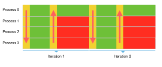
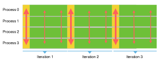
Figure 2: Flow diagrams of few iterations of DiSCO-S (top) and DiSCO-F (bottom). DiSCO-F uses less time for one iteration, due to the more efficient and balanced computation. Green boxes represent the processes are busy, while red boxes represent idle nodes. Yellow boxes show the status of communicating between all processes. Double arrows stand for ReduceAll operations. The thin red arrows represent a communication of few scalars only.

Table 3: Comparison of computation between different algorithms. For DiSCO-S, there exists large differences of computation between the master node and other node. But for DiSCO-F, each node will do exactly the same computation as each other.

	Operation	DiSCO-S	DiSCO-F
master	$y=Mx$	$1(\mathbb{R}^{d\times d}\cdot\mathbb{R}^{d})$	$1(\mathbb{R}^{d_{1}\times d_{1}}\cdot\mathbb{R}^{d_{1}})$
	$Mx=y$	1 ($\mathbb{R}^{d}$)	1 $(\mathbb{R}^{d_{1}})$
	$x+y$	4 ($\mathbb{R}^{d}$)	4 ($\mathbb{R}^{d_{1}}$)
	$x^{T}y$	4 ($\mathbb{R}^{d}$)	4 ($\mathbb{R}^{d_{1}}$)
nodes	$y=Mx$	1 $(\mathbb{R}^{d\times d}\cdot\mathbb{R}^{d})$	$1(\mathbb{R}^{d_{1}\times d_{i}}\cdot\mathbb{R}^{d_{i}})$
	$Mx=y$	0	1 $(\mathbb{R}^{d_{i}})$
	$x+y$	0	4 $(\mathbb{R}^{d_{i}})$
	$x^{T}y$	0	4 $(\mathbb{R}^{d_{i}})$

Table 4: Comparison of communication between different algorithms.

DiSCO-S	DiSCO-F	DANE	CoCoA+
$2\times\mathbb{R}^{d}$	$1\times\mathbb{R}^{n},2\times\mathbb{R}$	$2\times\mathbb{R}^{d}$	$1\times\mathbb{R}^{d}$

4 Woodbury Formula for solving $Ps=r$

In each iteration of Algorithms 2 and 3, we need to solve a linear system in the form of $Ps=r$, where $P\in\mathbb{R}^{d\times d}$ in Algorithm 2 and $P\in\mathbb{R}^{d_{i}\times d_{i}}$ for $i=1,2,...,m$ in Algorithm 3, which is usually very expensive. To solve it more efficiently, we can apply Woodbury Formula Press et al. (2007).

Notice that if we use $P$ defined in (5), $P$ can be considered as $\tau$ rank-1 updates on a diagnal matrix. For example, if $\phi(\cdot)$ is Quadtratic Loss, then

$$P=D+\frac{1}{\tau}\sum_{i=1}^{\tau}x_{i}x_{i}^{T}.$$ (8)

If $\phi(\cdot)$ is Logistic Loss, then

$$P=D+\frac{1}{\tau}\sum_{i=1}^{\tau}\frac{\exp(-w_{k}^{T}x_{i})}{(\exp(-w_{k}^{T}x_{i})+1)^{2}}x_{i}x_{i}^{T}.$$ (9)

In both cases, $D$ is the diagnal matrix with $D_{ii}=\lambda+\mu$ for $i=1,...,m$. Then we can follow the procedure to get the solution $s$.

Algorithm 4 Woodbury Formula to solve $Ps=r$

1:  Compute $z_{i}=\frac{1}{\lambda+\mu}x_{i}$ for $i=1,...,\tau$

2:  Let $Z=[z_{1},...,z_{\tau}]$, $X=[x_{1},...,x_{\tau}]$

3:  Compute $y=\frac{1}{\lambda+\mu}r$

4:  Solve the linear system $(I+X^{T}Z)v=X^{T}y$

5:  Return: $s=y-Xv$

Notes that $v\in\mathbb{R}^{\tau}$ and $\tau\ll d$ (in our experiments, $\tau=100$ usually works very well), step 4 can be done efficiently by any solver. In Section 5.3, we compare the effect of setting different values for $\tau$.

5 Numerical Experiments

We present experiments on several large real-world datasets distributed across multiple machines, running on an Amazon EC2 cluster with 4 instances. We show that DiSCO-F with a small $\tau$ converges to the optimal solution faster in terms of total rounds of communications compared to original DiSCO, DANE and CoCoA+ in most cases. Also, for the dataset with $d>n$, DiSCO-F will also dominate others in elapsed time. In Section 5.3, we compare the affects of preconditioning matrices with different values for $\tau$, and investigate that a small $\tau$ (around 100) would result in a impressive performance. In Section 5.4, we show that extra speed-up can be gained in some cases, by trying to shrink the number of samples that are used to compute Hessian.

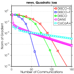
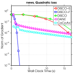
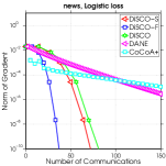
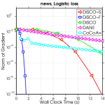
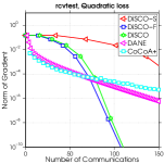
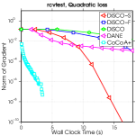
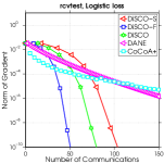
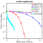
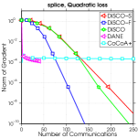
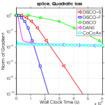
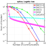
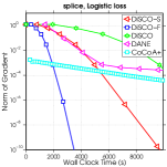
Figure 3: Norm of gradient vs. the round of communication, as well as norm of gradient vs. elapsed time in seconds for three datasets: news20 (top, $\lambda=1e-3$), rcv1.test (middle, $\lambda=1e-4$), splice-site.test (bottom, $\lambda=1e-6$) , each for two loss functions, Quadratic loss (left) and Logistic loss (right).

5.1 Implementation Details

We implement DiSCO and all other algorithms for comparison in C++, and run them in Amazon cluster using four m3.large EC2 instances. We apply all methods on applying Quadratic loss and Logistic loss in (P). A summary of the datasets used is shown in Table 5.

Table 5: Datasets used for numerical experiments.

Dataset	$n$	$d$	size(GB)
rcv1.test	677,399	47,236	1.21
news20	19,996	1,355,191	0.13
splice-site.test	4,627,840	11,725,480	273.4

5.2 Comparison of different algorithms

We compare the DiSCO-S, DiSCO-F, DiSCO, DANE and CoCOA+ directly using two datasets (new20 and rcv1.test) across two loss functions, where $\lambda$ is fixed to be $1e-4$. In DiSCO-S and DiSCO-F, we set $\tau=100$. In DiSCO and DANE, we apply Stochastic Average Gradient(SAG) Schmidt et al. (2013) to solve linear system $Ps=r$ and subproblem (3), respectively. Also, $\mu$ was set as $1e-2$ for both of them. In CoCoA+, SDCA was used as the solver for subproblems.

In Figure 3, we plot how the norm of the gradient of objective decreases with respective to the total number of communication and the elapsed time. In all the cases, DiSCO-F uses only half of the rounds of communications compared with DiSCO-S. Also, DiSCO-S often uses similar rounds of communications with the original DiSCO, which demonstrates the advantage of using preconditioning matrix based on only a small subset of the samples. Finally, DANE and CoCoA+ will decrease the norm of gradient very fast at the first few iterations, but the decreasing become much weaker as the iterations continue.

For the news20 ($d\gg n$) and splice-site.test ($d\sim n$) dataset, the DiSCO-F converges to the optimal solution with fewer iterations than all the other methods. The elapsed time for DiSCO-F is only 10% of DiSCO-S in the news20 case, due to the smaller size of the vector that needs to be communicated.

However, for the rcv.test dataset ($d<n$), even though DiSCO-F uses less number of communications, it tends to take longer time to reach an expected tolerance than DiSCO-S and CoCOA+. This is because the longer vectors ($\mathbb{R}^{n}$) that DiSCO-F needs to communicate in each CG iteration, compared with them in DiSCO-S and CoCOA+ ($\mathbb{R}^{d}$).

5.3 Impact of the Parameter $\tau$

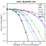
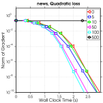
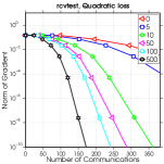
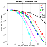
Figure 4: Comparison of different number of samples used in Preconditioning by running DiSCO-F.

In this section, we compare the performance of DiSCO-F algorithm of setting different $\tau$. If we apply methods described in Section 4, the parameter $\tau$ would determine how well the preconditioning matrix $P$ can approximate the true Hessian $H$. In a extreme case, if we only use one machine and $\tau=n$, then $\|P-H\|_{2}=0$ and each iteration of Algorithm 1 will only use 1 iteration of CG algorithm. However, too large $\tau$ will cause computation in Algorithm 4 quite expensive, thus resulting in long elapsed time. In our experiment, $\tau=500$ is even not acceptable, in terms of elapsed time.

As shown in Figure 4, the larger $\tau$ we use, the less total number of communications the algorithm takes to reach optimality. However, $\tau=100$ always leads to shorter time in both of these two datasets.

5.4 How Many Samples to Compute Hessian?

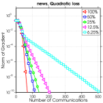
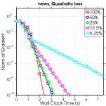
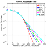
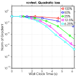
Figure 5: Comparison of different number of samples used in approximating Hessian by running DiSCO-F.

Notice that in step 4 of Algorithm 2 and 3, the product of the Hessian matrix and a vector need to be computed. In this section, We would like to try reducing the size of samples to compute Hessian. By doing so, we have to give up the current guaranteed complexity, since now the Hessian will be approximated. However, less elapsed time is expected if we choose proper size of samples. Due to the lack of theoretical analysis on this attempt, we only list the observation from the experiments.

For each iteration of Algorithm 1, we choose a subset of samples uniformly randomly to get the approximated Hessian. We try to choose subsets of samples whose sizes range from 100% to 6.25% of the entire dataset, as shown in Figure 5. For news20 dataset, such attempt will bring no benefits. The more samples we use, the less round of communications and elapsed time the algorithm spends to reach optimality. But for rcv1.test dataset, the elapsed time decreases as we reduce the number of samples to compute Hessian, which illustrates that using only a small portion of samples will be helpful to get enough information of Hessian in each iteration.

The reason of this result might be for the dataset with a rather large number of features (news20), ignoring some samples will result in lots of relationship between features missed. For the dataset with rather small number of features (rcv1), the Hessian can be approximated well by only a small subset of data.

6 Conclusion

In conclusion, based on the DiSCO algorithm Zhang & Xiao (2015), we study inexact dumped Newton method implemented in a distributed way. We found that by partitioning the dataset by features, the number of communications can be reduced and the computation in each machine becomes more balanced. Also, we shrink the size of samples to generate the preconditioning matrix, which greatly improves the efficiency of solving the linear system in CG. Our experimental results show significant speedups over previous methods, including the original DiSCO algorithm as well as other state-of-the-art methods.

References

- Agarwal & Duchi (2011) Agarwal, Alekh and Duchi, John C. Distributed delayed stochastic optimization. In Advances in Neural Information Processing Systems, pp. 873–881, 2011.
- Bertsekas & Tsitsiklis (1989) Bertsekas, Dimitri P and Tsitsiklis, John N. Parallel and distributed computation: numerical methods. Prentice-Hall, Inc., 1989.
- Boyd et al. (2011) Boyd, Stephen, Parikh, Neal, Chu, Eric, Peleato, Borja, and Eckstein, Jonathan. Distributed optimization and statistical learning via the alternating direction method of multipliers. Foundations and Trends® in Machine Learning, 3(1):1–122, 2011.
- Bradley et al. (2011) Bradley, Joseph K, Kyrola, Aapo, Bickson, Danny, and Guestrin, Carlos. Parallel coordinate descent for l1-regularized loss minimization. arXiv preprint arXiv:1105.5379, 2011.
- Csiba et al. (2015) Csiba, Dominik, Qu, Zheng, and Richtárik, Peter. Stochastic dual coordinate ascent with adaptive probabilities. arXiv preprint arXiv:1502.08053, 2015.
- Defazio et al. (2014) Defazio, Aaron, Bach, Francis, and Lacoste-Julien, Simon. Saga: A fast incremental gradient method with support for non-strongly convex composite objectives. In Advances in Neural Information Processing Systems, pp. 1646–1654, 2014.
- Dekel et al. (2012) Dekel, Ofer, Gilad-Bachrach, Ran, Shamir, Ohad, and Xiao, Lin. Optimal distributed online prediction using mini-batches. The Journal of Machine Learning Research, 13(1):165–202, 2012.
- Deng & Yin (2012) Deng, Wei and Yin, Wotao. On the global and linear convergence of the generalized alternating direction method of multipliers. Journal of Scientific Computing, pp. 1–28, 2012.
- Duchi et al. (2013) Duchi, John C, Jordan, Michael I, and McMahan, H Brendan. Estimation, Optimization, and Parallelism when Data is Sparse. In NIPS, 2013.
- Forero et al. (2010) Forero, Pedro A, Cano, Alfonso, and Giannakis, Georgios B. Consensus-based distributed support vector machines. The Journal of Machine Learning Research, 11:1663–1707, 2010.
- Hsieh et al. (2008) Hsieh, Cho-Jui, Chang, Kai-Wei, Lin, Chih-Jen, Keerthi, S Sathiya, and Sundararajan, Sellamanickam. A dual coordinate descent method for large-scale linear svm. In Proceedings of the 25th international conference on Machine learning, pp. 408–415. ACM, 2008.
- Jaggi et al. (2014) Jaggi, Martin, Smith, Virginia, Takác, Martin, Terhorst, Jonathan, Krishnan, Sanjay, Hofmann, Thomas, and Jordan, Michael I. Communication-efficient distributed dual coordinate ascent. In Advances in Neural Information Processing Systems, pp. 3068–3076, 2014.
- Johnson & Zhang (2013) Johnson, Rie and Zhang, Tong. Accelerating stochastic gradient descent using predictive variance reduction. NIPS, pp. 315–323, 2013.
- Konečný et al. (2014) Konečný, Jakub, Liu, Jie, Richtárik, Peter, and Takáč, Martin. mS2GD: Mini-batch semi-stochastic gradient descent in the proximal setting. arXiv preprint arXiv:1410.4744, 2014.
- Lee & Roth (2015) Lee, Ching-Pei and Roth, Dan. Distributed box-constrained quadratic optimization for dual linear SVM. ICML, 2015.
- Liu et al. (2014) Liu, Ji, Wright, Stephen J, Ré, Christopher, Bittorf, Victor, and Sridhar, Srikrishna. An Asynchronous Parallel Stochastic Coordinate Descent Algorithm. In ICML, 2014.
- Ma et al. (2015a) Ma, Chenxin, Konečnỳ, Jakub, Jaggi, Martin, Smith, Virginia, Jordan, Michael I, Richtárik, Peter, and Takáč, Martin. Distributed optimization with arbitrary local solvers. arXiv preprint arXiv:1512.04039, 2015a.
- Ma et al. (2015b) Ma, Chenxin, Smith, Virginia, Jaggi, Martin, Jordan, Michael I, Richtárik, Peter, and Takáč, Martin. Adding vs. averaging in distributed primal-dual optimization. In ICML 2015 - Proceedings of the 32th International Conference on Machine Learning, volume 37, pp. 1973–1982. JMLR, 2015b.
- Marecek et al. (2014) Marecek, Jakub, Richtárik, Peter, and Takác, Martin. Distributed block coordinate descent for minimizing partially separable functions. Numerical Analysis and Optimization 2014, Springer Proceedings in Mathematics and Statistics, 2014.
- Nitanda (2014) Nitanda, Atsushi. Stochastic proximal gradient descent with acceleration techniques. In Advances in Neural Information Processing Systems, pp. 1574–1582, 2014.
- Niu et al. (2011) Niu, Feng, Recht, Benjamin, Ré, Christopher, and Wright, Stephen J. Hogwild!: A Lock-Free Approach to Parallelizing Stochastic Gradient Descent. In NIPS, 2011.
- Press et al. (2007) Press, William H, Teukolsky, Saul A, Vetterling, William T, and Flannery, Brian P. Numerical recipes: the art of scientific computing. 2007.
- Qu et al. (2015) Qu, Zheng, Richtárik, Peter, and Zhang, Tong. Quartz: Randomized dual coordinate ascent with arbitrary sampling. In Advances in Neural Information Processing Systems, pp. 865–873, 2015.
- Recht et al. (2011) Recht, Benjamin, Re, Christopher, Wright, Stephen, and Niu, Feng. Hogwild: A lock-free approach to parallelizing stochastic gradient descent. In Advances in Neural Information Processing Systems, pp. 693–701, 2011.
- Richtárik & Takáč (2013) Richtárik, Peter and Takáč, Martin. Distributed coordinate descent method for learning with big data. arXiv preprint arXiv:1310.2059, 2013.
- Rodgers (1985) Rodgers, David P. Improvements in multiprocessor system design. In ACM SIGARCH Computer Architecture News, volume 13, pp. 225–231. IEEE Computer Society Press, 1985.
- Roux et al. (2012) Roux, Nicolas L, Schmidt, Mark, and Bach, Francis R. A stochastic gradient method with an exponential convergence _rate for finite training sets. In Advances in Neural Information Processing Systems, pp. 2663–2671, 2012.
- Schmidt et al. (2013) Schmidt, Mark, Roux, Nicolas Le, and Bach, Francis. Minimizing finite sums with the stochastic average gradient. arXiv:1309.2388, 2013.
- Shalev-Shwartz et al. (2011) Shalev-Shwartz, Shai, Singer, Yoram, Srebro, Nathan, and Cotter, Andrew. Pegasos: Primal estimated sub-gradient solver for svm. Mathematical programming, 127(1):3–30, 2011.
- Shamir & Srebro (2014) Shamir, Ohad and Srebro, Nathan. Distributed stochastic optimization and learning. In Communication, Control, and Computing (Allerton), 2014 52nd Annual Allerton Conference on, pp. 850–857. IEEE, 2014.
- Shamir et al. (2013) Shamir, Ohad, Srebro, Nathan, and Zhang, Tong. Communication efficient distributed optimization using an approximate newton-type method. arXiv preprint arXiv:1312.7853, 2013.
- Takáč et al. (2013) Takáč, Martin, Bijral, Avleen, Richtárik, Peter, and Srebro, Nathan. Mini-batch primal and dual methods for SVMs. ICML, 2013.
- Takáč et al. (2015) Takáč, Martin, Richtárik, Peter, and Srebro, Nathan. Distributed mini-batch SDCA. arXiv preprint arXiv:1507.08322, 2015.
- Yang (2013) Yang, Tianbao. Trading computation for communication: Distributed stochastic dual coordinate ascent. In Advances in Neural Information Processing Systems, pp. 629–637, 2013.
- Yang et al. (2013) Yang, Tianbao, Zhu, Shenghuo, Jin, Rong, and Lin, Yuanqing. Analysis of distributed stochastic dual coordinate ascent. arXiv preprint arXiv:1312.1031, 2013.
- Zhang & Xiao (2015) Zhang, Yuchen and Xiao, Lin. Communication-efficient distributed optimization of self-concordant empirical loss. arXiv preprint arXiv:1501.00263, 2015.