Redshift-space distortions around voids

Abstract

We have derived estimators for the linear growth rate of density fluctuations using the cross-correlation function (CCF) of voids and haloes in redshift space. In linear theory, this CCF contains only monopole and quadrupole terms. At scales greater than the void radius, linear theory is a good match to voids traced out by haloes; small-scale random velocities are unimportant at these radii, only tending to cause small and often negligible elongation of the CCF near its origin. By extracting the monopole and quadrupole from the CCF, we measure the linear growth rate without prior knowledge of the void profile or velocity dispersion. We recover the linear growth parameter $\beta$ to 9% precision from an effective volume of $3(\,h^{-1}{\rm Gpc})^{3}$ using voids with radius >25$\,h^{-1}{\rm Mpc}$. Smaller voids are predominantly sub-voids, which may be more sensitive to the random velocity dispersion; they introduce noise and do not help to improve measurements. Adding velocity dispersion as a free parameter allows us to use information at radii as small as half of the void radius. The precision on $\beta$ is reduced to 5%. Voids show diverse shapes in redshift space, and can appear either elongated or flattened along the line of sight. This can be explained by the competing amplitudes of the local density contrast, plus the radial velocity profile and its gradient. The distortion pattern is therefore determined solely by the void profile and is different for void-in-cloud and void-in-void. This diversity of redshift-space void morphology complicates measurements of the Alcock-Paczynski effect using voids.

1 Introduction

Using redshift-space distortions (RSD) to probe the growth of large-scale structure has been a target for cosmological research since the first prediction of the effect (Kaiser, 1987) and observational RSD studies have been pursued for over two decades (e.g. Hamilton, 1992; Cole et al., 1994, 1995; Peacock et al., 2001; Beutler et al., 2012; Reid et al., 2012; Blake et al., 2012; de la Torre et al., 2013; Samushia et al., 2014; Howlett et al., 2015; Okumura et al., 2016). The pairwise galaxy-galaxy power spectrum or correlation function approaches the prediction of linear theory at very large scales, but in the quasi-linear and non-linear regime, more sophisticated models are needed to account for non-linear growth (e.g. Scoccimarro, 2004; Matsubara, 2008; Taruya et al., 2009; Percival & White, 2009; Taruya et al., 2010; Seljak & McDonald, 2011; Jennings et al., 2011; Gil-Marín et al., 2012; Okumura et al., 2012; de la Torre & Guzzo, 2012; Valageas et al., 2013; Okumura et al., 2015); with care, it is possible to recover the linear growth rate to 2% precision by including this small-scale information (Reid et al., 2014). This average growth is extracted from the pairwise galaxy-galaxy correlations, which sample peaks and troughs of the matter density field; it remains an open question, at least from the observational point of view, how the growth of structure depends on the environment. At a minimum, the growth of density perturbations is expected to be more rapid in superclusters and lower in voids, simply because these regions resemble universes with different cosmological parameters. The scales where such non-linear growth effects become important will probably differ between different environments. But the environmental dependence of the growth of structure may have a more fundamental significance, since it could encode information about non-standard theories of gravity. Measurements for the growth at different environment can thus be used as a test for departures from Einstein gravity. As discussed below, such deviations are frequently expected to be stronger where the matter density is low, which leads us to investigate the growth of structure in void environments.

Cosmic voids are large underdense regions of the universe that are devoid of galaxies. Voids in large-scale structure have great potential in constraining cosmology and gravity via the following observables: the Alcock-Paczynski (AP) test (Alcock & Paczynski, 1979; Lavaux & Wandelt, 2012); stacking of voids for the integrated Sachs-Wolfe (ISW) effect (Sachs & Wolfe, 1967; Granett et al., 2008; Cai et al., 2014a, b); weak lensing measurement of the matter distribution in voids (Higuchi et al., 2013; Krause et al., 2013; Cai et al., 2015; Clampitt & Jain, 2015; Gruen et al., 2016); void ellipticity as a probe for the dark energy equation of state (Lee & Park, 2009; Bos et al., 2012); void density profiles and number counts as a probe of modified gravity (Clampitt et al., 2013; Lam et al., 2015; Cai et al., 2015; Zivick et al., 2015; Barreira et al., 2015); coupled dark energy (Pollina et al., 2016); the nature of dark matter (Yang et al., 2015); massive neutrino (Massara et al., 2015); and Baryon Acoustic Oscillations in void clustering (Kitaura et al., 2016; Liang et al., 2016).

The growth of structure around cosmic voids is fundamentally related to the detailed understanding of some of these observables. For example, the AP measurement using cosmic voids makes the underlying assumption that stacked voids are of the same size in both the transverse and line-of-sight (LOS) direction if the assumed cosmology is correct – but this assumption is violated by redshift-space distortions (Lavaux & Wandelt, 2012; Sutter et al., 2014). The effect of peculiar velocities on the observed configuration of voids must be understood in order to obtain unbiased cosmological AP measurements. Another example is that the ISW signal associated with cosmic voids is determined by the local growth rate, which is affected by possibly nonlinear density and velocity structure.

We will focus here on extracting the growth rate around voids. The void-mass (or void-galaxy) correlations in redshift space are the tool we will employ for the measurement. We will follow closely the methodology of conventional redshift-space distortion analyses to derive the mapping between redshift-space and real-space clustering for voids. This will give us a comprehensive picture of how the redshift-space void-mass correlation function is affected by different aspects of the density and velocities, which will be essential for understanding how the AP measurement with voids is affected by redshift-space distortions.

In Section 2, we derive the expression for the redshift-space void-mass correlation function using linear theory. In Section 3 we then give examples to explain the complexity of void-mass correlation function. Section 4 focuses on developing a method for measuring the growth around voids and testing it using an N-body simulation. During the preparation of this manuscript, Hamaus et al. (2015) released a paper on the same topic; we compare our results at the end of Section 4. We sum up and draw conclusions in Section 5.

2 Redshift-space distortions around voids

Although our goal is to derive the expression for the void-mass correlation function in redshift space in this section, there is no requirement that the system must be underdense. The derivation and the results are therefore relevant to the overdense case, i.e. to the halo-mass correlation function – see e.g. Croft et al. (1999); Zu & Weinberg (2013).

2.1 Linear theory

The difference between the redshift-space void-mass correlation function and the pairwise galaxy-galaxy correlation function is that we are considering the relative peculiar velocities of dark matter (or dark matter haloes) with respect to one central point, the void centre. The bulk motion of voids will therefore not affect the void-mass correlation function within the scales where the bulk velocity field can be considered to be coherent (see Section 4 for further discussion on this point). With the plane-parallel approximation, $|v/r_{c}aH|\ll 1$ where $v$ is the peculiar velocity of dark matter, $r_{c}$ is its comoving distance from the observer, $a$ is the scale factor of the universe and $H$ is the Hubble constant at $a$, the mapping between redshift-space and real-space overdensities is

$$1+\delta^{s}({\bf r})=[1+\delta({\bf r})]\;[1+u^{\prime}({\bf r})]^{-1},$$ (1)

where $\delta({\bf r})=\rho({\bf r})/\bar{\rho}-1$ with $\bar{\rho}$ being the mean density of the universe and $\rho({\bf r})$ the matter density at ${\bf r}$, which is defined with an origin at the void centre. For $\delta({\bf r})\ll 1$ and $|\partial v({\bf r})/\partial{\bf r}|\ll aH$, to linear order we have

$$\delta^{s}({\bf r})=\delta({\bf r})-u^{\prime}({\bf r}).$$ (2)

The distortion term $u^{\prime}({\bf r})$ is the gradient of the radial velocity profile around the void centre $v({\bf r})$ projected along the line of sight:

$$u^{\prime}(\mathbf{r}) ={\bf\hat{z}}\cdot\frac{1}{aH}\frac{\partial\left[{\bf\hat{z}\cdot\hat{r}}v({\bf r})\right]}{\partial{\bf r}}$$ (3)

$$=(1-\mu^{2})\frac{1}{aH}\frac{v({r})}{r}+\mu^{2}\frac{1}{aH}\frac{\partial v({r})}{\partial r},$$ (4)

where ${\bf\hat{z}}$ is the unit vector along the line of sight, $\mu=\cos(\theta)$ and $\theta$ is the angle subtended between ${\bf r}$ and ${\bf\hat{z}}$. In linear theory,

$$v(r) =-\frac{1}{3}raH\bar{\delta}(r)f;$$ (5)

$$\bar{\delta}(r) =\frac{3}{r^{3}}\int^{r}_{0}\delta(r^{\prime})r^{\prime 2}dr^{\prime}$$ (6)

(Peebles, 1993), where $f\equiv d\ln D/d\ln a$ is the linear growth rate, and $D$ is the linear growth factor. It is straightforward to show that

$$\frac{\partial v(r)}{\partial r}=-faH\left[\delta(r)-\frac{2}{3}\bar{\delta}(r)\right].$$ (7)

Eq. (2) then takes the form

$$\xi_{\rm vm}^{s}({\bf r})=\delta(r)+\frac{1}{3}f\bar{\delta}(r)+f\mu^{2}[\delta(r)-\bar{\delta}(r)],$$ (8)

where instead of $\delta^{s}({\bf r})$, we have used the notation $\xi_{\rm vm}^{s}({\bf r})$. This is because the conditional density fluctuation is identical in meaning to the cross-correlation function, which gives the fractional fluctuation in the number of cross-pairs. The above equation therefore shows that the void-mass correlation function in redshift space contains only monopole and quadrupole terms. This is different from the pairwise galaxy-galaxy autocorrelation function, where there is also a hexadecapole moment. We discuss the reason for this distinction in greater depth in Section 4.

2.2 Quasi-linear model

The above expression is only valid on the assumption that $\delta\ll 1$ and that any random dispersion in velocity is small. These assumptions can be relaxed, which leads to the quasi-linear model (Peebles, 1993; Fisher et al., 1994a, b; Fisher, 1995). In this model, the redshift-space correlation function is expressed as the convolution of its real-space version with the probability distribution function for velocities along the LOS:

$$1+\xi_{\rm vm}^{s}(r_{\sigma},r_{\pi})= \int_{-\infty}^{\infty}\left[1+\delta\left(r_{\sigma},r_{\pi}-\frac{v_{\pi}}{aH}\right)\right]\times p(v_{\pi})dv_{\pi}$$

$$= \int_{-\infty}^{\infty}\left[1+\delta\left(r_{\sigma},r_{\pi}-\frac{v_{\pi}}{aH}\right)\right]\times$$

$$\frac{1}{\sqrt{2\pi}\sigma_{\rm v}}\exp\left(-\frac{\left[(v_{\pi}-v(r)\mu\right]^{2}}{2\sigma_{\rm v}^{2}(r)}\right)dv_{\pi},$$ (9)

where $\mu=(r_{\pi}-v_{\pi}/aH)/r$, $r^{2}=r_{\sigma}^{2}+(r_{\pi}-v_{\pi}/aH)^{2}$. When $\delta\ll 1$ and $\sigma_{\rm v}(r)$ is small, linear theory is well recovered (Peebles, 1993; Fisher, 1995), as we have also explicitly checked.

With the assumption that galaxies or haloes are linearly biased tracers of dark matter, we can generalise this result to give the void-galaxy or void-halo correlation function by replacing $f$ with $\beta$ in the above equation, where $\beta=f/b$, and $b$ is the linear bias for galaxies or haloes.

Figure 1: Top-left: redshift-space void-halo correlation functions. In this example, only voids-in-clouds defined as $\bar{\xi}^{s}_{0}(r=3r_{\rm v})>0$ are selected from the sample. Black contours and the underlying colour image are results from our simulation. White-dashed contours are from the best-fit linear model. Top-right: The distortions to the correlation function due to peculiar velocities from the linear model. This is obtained by subtracting the real-space correlation function from its redshift-space version. Bottom-left: Moments of the real and redshift-space void-halo correlation functions. $\xi_{0}$ shown by the black dashed curve is the real-space monopole measured from our simulation using 3D positions of haloes in real space. It is in essence the stacked void profile in real space. The red-dashed curve ($\xi_{0}^{s}$ ) is the redshift-space void profile measured from the 3D positions of haloes in redshift space. The red dots are the same as the red-dashed curve except that they are the monopoles extracted from the correlation function shown on the top-left panel. The orange (quadrupole $\xi_{2}^{s}$) and blue dots ($\xi_{0}^{s}-\bar{\xi}^{s}_{0}$) are measurements from the correlation function, and the dashed curves of the same colours are predictions from linear theory. The green dotted curve is $\bar{\xi}^{s}_{0}$, the cumulative void profile. Bottom-right: radial velocity profile from void centres (solid black) and its dispersion (black dashed curve).

Figure 2: The same as Fig. 1 but showing all voids with radii between 25-35$\,h^{-1}{\rm Mpc}$.

Figure 3: The same as Fig. 1 but showing all voids with radii between 35-60$\,h^{-1}{\rm Mpc}$.

2.3 Simulation set up and void definition

We employ an N-body simulation of a $\Lambda$CDM model to test the performance of the linear model and later to test our estimator to extract the linear growth from voids. The simulation was run with the following parameters: $\Omega_{\rm m}=0.24$, $\Omega_{\rm\Lambda}=0.76$, $h=0.73$, and $n_{\rm s}=0.958$ and $\sigma_{8}=0.80$ (Li et al., 2013). The volume of the simulation box is $(1\,h^{-1}{\rm Gpc})^{3}$ We use all haloes above a minimum halo mass of $M_{\rm min}=10^{12.8}\,h^{-1}{\rm M_{\odot}}$ to ensure that each halo contains at least 100 particles. We choose to test our analysis at $z=0$, where our halo number density is 3.1$\times 10^{-4}(\,h^{-1}{\rm Mpc})^{-3}$, and the linear halo bias of our halo population is $b=1.7$. Voids are found in the halo field with the spherical underdensity algorithm described in Cai et al. (2015), which is based on the algorithm of Padilla et al. (2005). The algorithm works on the halo catalogue in the simulation box by growing maximal spheres from a set of grid points within which the number density of haloes satisfies the criterion $\Delta\leq 0.2$. Void candidates are ranked in decreasing order of radius. Spheres that overlap with a neighbour by a radius more than 50% of the sum of their radii are rejected. Note that this does not mean that no sub-voids are allowed. A small void contained in a large one can still pass this selection criterion, and we expect the fraction of such sub-voids to increase for smaller voids.

We choose one of the major axes of the simulation box as the line-of-sight direction and perturb halo positions with their peculiar velocities assuming the plane-parallel approximation:

$$s=r+v_{z}/aH,$$ (10)

where $s$ and $r$ is the redshift-space and real-space comoving coordinates of haloes. $v_{z}$ is the line-of-sight peculiar velocity. We view our voids along the three major axes of the simulation box, which effectively increases our sample by a factor of 3. All figures in our paper are made in this way unless specified.

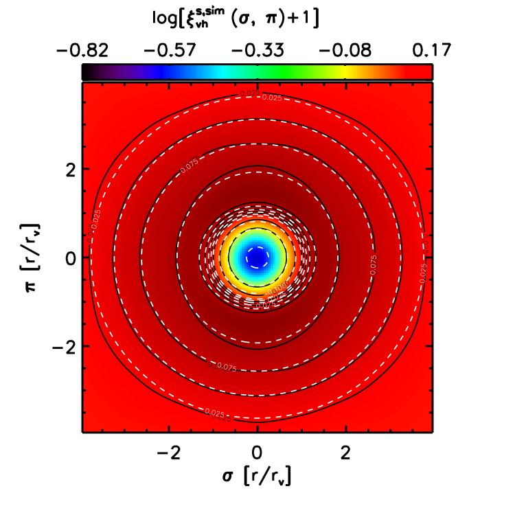
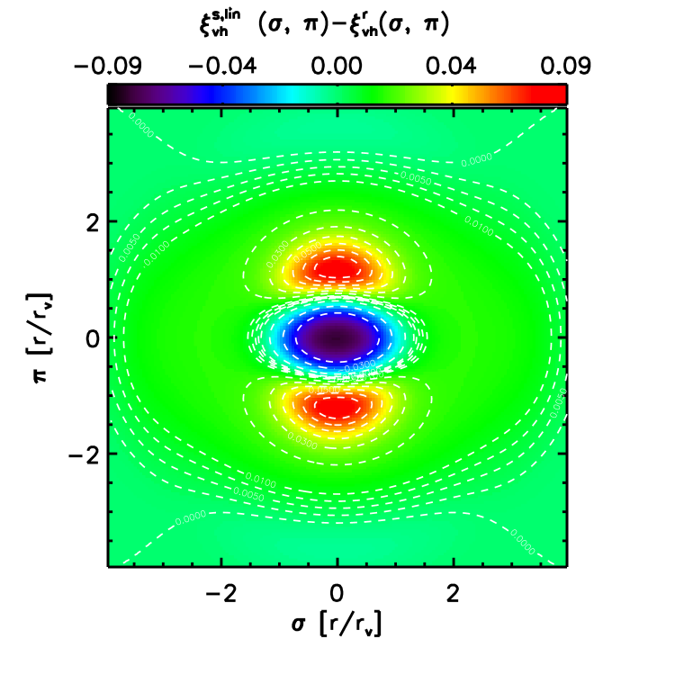
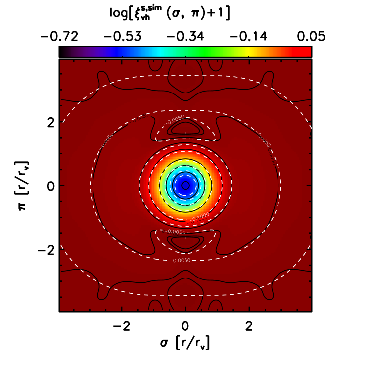
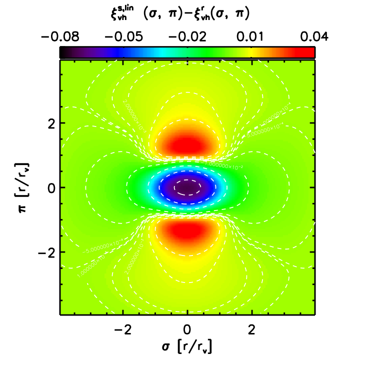
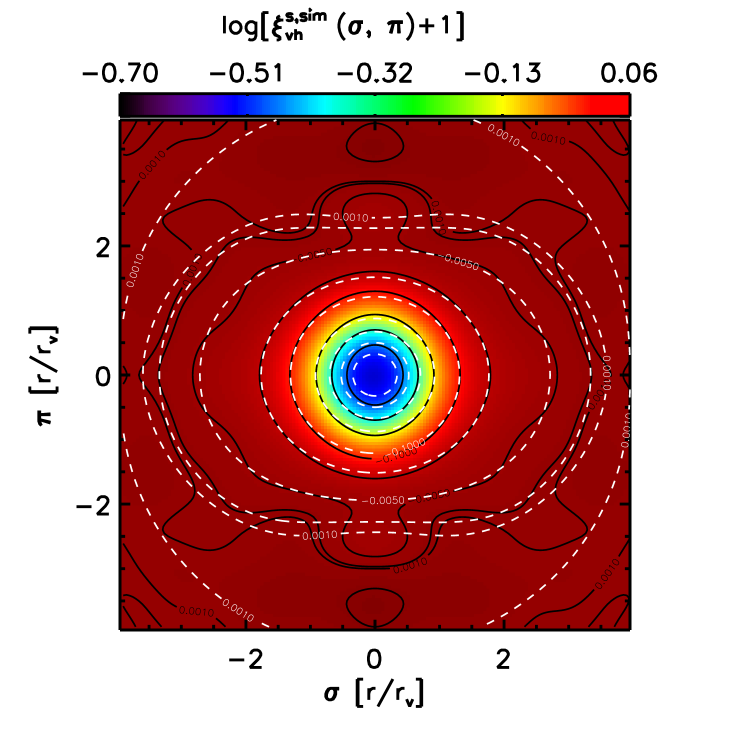
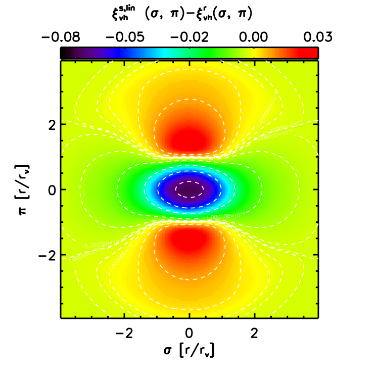
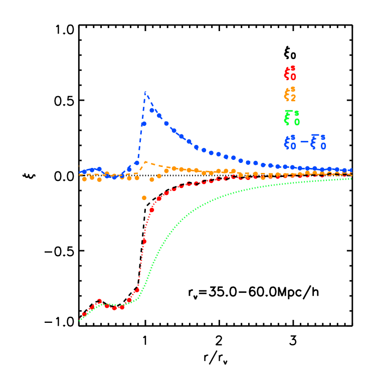
With the halo field in redshift space, we measure the redshift-space void-halo correlation function $\xi^{s}{(\sigma,\pi)}$. We rescale the correlation function for each void by the void radius along both the $\sigma$ and $\pi$ directions. Examples of the stacked correlation function are shown in the top-left panel of Fig. 1, 2, 3 & 4. For all cases, there are very good agreements between the black contours from simulation with the white contours from the linear model. A more quantitative comparison of model and numerical data will be conducted in Section 4.

3 Distortion patterns: Elongation vs. Flattening

Before we move on to write down estimators for the growth based on the above models, we first use these models and the simulation to understand the distortion pattern of voids in redshift space, i.e. whether a spherical void should appear elongated or flattened along the LOS. This is particularly relevant for the AP test, which relies on measuring the apparent size of voids along the LOS and transverse to it.

In the linear model, the redshift-space void configuration depends on the real-space void profile, the radial velocity profile as well as its gradients [Eq. (2) & (4)]. From the linear model [Eq. (8)], the distortion pattern of voids depends solely on the real-space void profiles, as the real velocity and its gradients are both determined by the void profile. It can be understood by examining the correlation function in the two extreme directions: LOS versus transverse to the LOS. When $\mu^{2}\ll 1$, the correlation function can be approximated by its transverse version, i.e.

$$\xi_{\rm vm}^{s}({\bf r})=\delta(r)+\frac{1}{3}f\bar{\delta}(r);$$ (11)

When $\mu^{2}\approx 1$, the correlation function can be approximated by its LOS version, i.e.

$$\xi_{\rm vm}^{s}({\bf r})=(1+f)\delta(r)-\frac{2}{3}f\bar{\delta}(r).$$ (12)

Since $\bar{\delta}(r)$ is always negative within the void radius by definition, the second term in Eq. (11) is of the same sign as the first term, and it acts to deepen the density contrast in the transverse direction. The second term in Eq. (12), including the negative sign has the opposite sign with respect to the first term, which itself is boosted by a factor of $(1+f)$. Hence, the amplitude of clustering along the LOS can be enhanced or reduced, depending on the competing amplitudes of $f\delta$ versus $\frac{2}{3}f\bar{\delta}$. For haloes, $f\delta$ becomes $\beta\delta$, and for massive haloes with a linear bias of $\approx 2$, $\beta$ is relatively small. The amplitude of $f\delta$ is usually smaller than $\frac{2}{3}\bar{\delta}$ at $r<r_{\rm v}$. Hence the second term of Eq. (12) cancels part of the first term, making the density contrast shallower along the LOS. Both these two effects act to flatten the void. Therefore, voids usually appear flattened in redshift space within the void radius. This is visualised in the top-right panels of Figs 1, 2 & 3. At $r<r_{\rm v}$, all the three stacked voids appear flattened, though the amplitudes of the distortion patterns are relatively weak and difficult to see on the top-left panels where the full correlation functions from simulation and the best-fit models are shown.

The distortion feature can also be understood by differencing the transverse correlation function by its LOS version, i.e. subtracting Eq. (11) by Eq. (12), which yields $f[\bar{\delta}(r)-\delta(r)]$. Within $r_{\rm v}$, $\delta(r)$ and $\bar{\delta}(r)$ are both negative and the amplitude of the latter is larger. Therefore, $f[\bar{\delta}(r)-\delta(r)]<0$, i.e. the correlation function is more negative at the transverse direction than along the LOS. So the void is flattened.

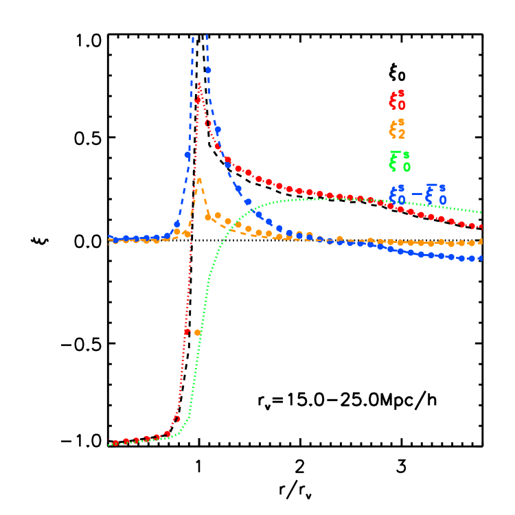
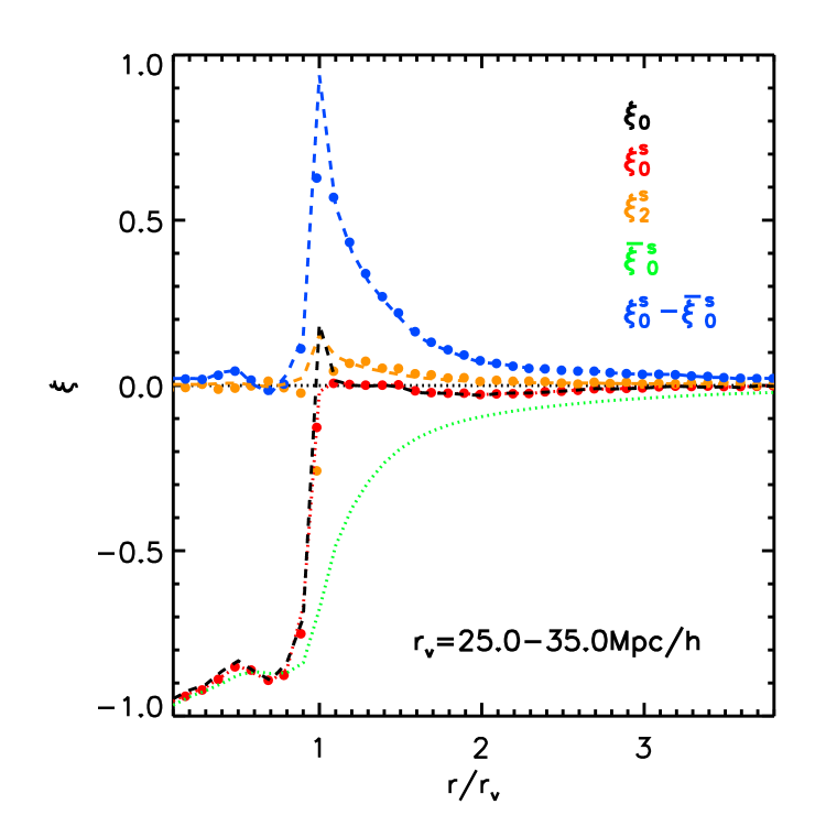
At radii greater than $r_{\rm v}$, the distortion pattern depends on the type of voids. Uncompensated voids are typically embedded in larger-scale underdense environments, which also expand in an unbound manner. These are the so-called voids-in-voids (Sheth & van de Weygaert, 2004). Here, $\bar{\delta}(r)$ is negative up to large radii. If the differential profile $\delta(r)$ also stays negative at large radii, the same flattening feature is expected. But if $\delta(r)$ turns positive at some large radius, the distortion pattern becomes elongated. For uncompensated voids, this happens typically at large radii. So the general picture for uncompensated voids in redshift space is flattening at relatively small radii (greater than $r_{\rm v}$) and elongation at the very large radii when $\delta(r)$ becomes positive. Fig. 3 gives an example of this kind. On the bottom-left panel, the cumulative void profile $\bar{\delta}(r)$ is negative up to $4r_{\rm v}$. The differential void profile indicated by the red dots and red dashed curves remains negative at $r<2r_{\rm v}$ and it become weakly positive at $r>2r_{\rm v}$. In the top panel, the flattening feature is seen up to twice the void radius; it then becomes elongated at larger radii as expected.

In contrast, over-compensated voids are likely to be embedded in overdense environments: these are voids-in-clouds (Sheth & van de Weygaert, 2004). Here, $\bar{\delta}(r)$ is negative within the compensation radius $r_{\rm com}$, becoming positive for $r>r_{\rm com}$. The differential profile $\delta(r)$ must then become positive at $r<r_{\rm com}$. Therefore, at $r<r_{\rm v}$, the void appears flattened; between $r_{\rm v}<r<r_{\rm com}$ it is elongated. At $r>r_{\rm com}$, the shape becomes flattened again as both $\delta(r)$ and $\bar{\delta}(r)$ remain positive, which is essentially the same as the flattening feature in overdensities. An example is given in Fig. 1, where we have selected voids from our simulation with $\bar{\delta}(r)>0$ at $r=r_{\rm v}$ to make sure they are voids surrounded by large-scale overdense environments. The over-compensation property of the stacked voids is also reflected by the fact that the mean radial velocity becomes negative at $r>1.7r_{\rm v}$, as shown in the bottom-right panel of Fig. 1.

When adding a dispersion in velocity according to the quasi-linear model shown in Section 2.2, we find that the correlation functions are weakly elongated along the LOS, and the effect is stronger at $r<r_{\rm v}$. In some cases where the dispersion is dominant over the mean streaming velocity, the interior of voids becomes elongated rather than flattened. At larger radii, the impact of velocity dispersion is found to be negligible. It is worth noting that, according to the quasi-linear model, the interior of the void may also appear elongated when the amplitude of $\delta$ is relatively large, i.e. $\delta\sim-1$, where the linear model is no longer accurate.

In summary, peculiar velocities cause complex distortion patterns for voids in redshift space, which can largely be understood using linear theory. Voids usually appear flattened within the radius of underdensity according to linear theory, but can be elongated when velocity dispersion is non-negligible; they may be elongated or flattened at large radii. This behaviour is mostly determined by the density profile, as the impact of velocity dispersion is very small at larger radii. In some cases, the transition between flattening and elongation is very abrupt. This is different from the relatively simple distortion patterns for overdensities, where infall streaming motion causes flattening on large scales and random velocity dispersion induces Finger-of-God-like elongation on small scales. This suggests that the effect of redshift-space distortion on the AP measurement using voids depends strongly on both the void population and the radius where the size of the void is taken. It is perhaps over-simplistic to apply a single stretching factor to correct for this effect, as was done in Sutter et al. (2014), given the wide range of void profiles encountered in practice.

The fact that the impact of velocity dispersion is small at large radii suggest that the linear model without velocity dispersion may be sufficient to provide good fit for the correlation function at $r>r_{\rm v}$. As we will show in the next section, allowance for velocity dispersion is needed only when fitting at $r<r_{\rm v}$,

4 measuring the growth rate

4.1 The growth estimator

Following Hamilton (1992, 1998), we can write down the following pair of equations for the void-mass correlation function:

$$\xi_{0}^{s}(r)-\frac{3}{r^{3}}\int_{0}^{r}\xi^{s}_{0}(r^{\prime})r^{\prime 2}dr^{\prime} =\left(1+\frac{f}{3}\right)[\xi(r)-\bar{\xi}(r)]$$ (13)

$$\xi_{2}^{s}(r) =\frac{2f}{3}[\xi(r)-\bar{\xi}(r)],$$ (14)

where $\bar{\xi}(r)=(3/r^{3})\int_{0}^{r}\xi(r^{\prime})r^{\prime 2}dr^{\prime}$. Since the hexadecapole is zero, we have

$$\xi^{s}(r,\mu) =\xi_{0}^{s}(r)+\frac{3\mu^{2}-1}{2}\xi^{s}_{2}(r)$$ (15)

$$=\left(1+\frac{f}{3}\right)\xi(r)+\frac{f(3\mu^{2}-1)}{3}[\xi(r)-\bar{\xi}(r)]$$

$$=\xi(r)+\frac{1}{3}f\bar{\xi}(r)+f\mu^{2}[\xi(r)-\bar{\xi}(r)]$$

The above expression matches to Eq. (8) because the void-mass correlation function $\xi(r)$ is essentially the real-space density profile of voids $\delta(r)$; thus $\bar{\xi}(r)=\bar{\delta}(r)$.

With the above pair of moments of the correlation function, we can estimate the growth rate using the estimator

$$\tilde{G}(f) =\frac{\xi_{2}^{s}(r)}{\xi_{0}^{s}(r)-\frac{3}{r^{3}}\int_{0}^{r}\xi^{s}_{0}(r^{\prime})r^{\prime 2}dr^{\prime}}$$ (16)

$$=\frac{2f}{3+f}.$$ (17)

The multipoles of correlation function can be obtained by

$$\xi^{s}_{\ell}(r)=\int_{0}^{1}\xi^{s}(r,\mu)(1+2\ell)P_{\ell}(\mu)d\mu,$$ (18)

where $P_{0}(\mu)=1$ and $P_{2}(\mu)=\frac{1}{2}(3\mu^{2}-1)$.

Figure 4: Top-left: The void-halo correlation function in redshift space. The black contours give results from the simulation and the white contours are the best-fit linear model. Top-right: Cross-correlation coefficients of the covariance matrix shown in Eq. (25). Bottom-left: the upper panel shows the monopole and quadrupole moments of the redshift space correlation function. The lower panel shows the ratio of the quadrupole versus monopole. The black curve is from taking all measurements of voids along three different major axes of the simulation box, with the shaded region showing the error on the mean. The other three curves represent results from viewing the simulation along three different major axes. The black filled circle with error bars is the best-fit value from viewing voids along three different directions. The red, blue and orange filled circles and errors are from individual viewing directions. They are slightly offset from each other to aid visibility. The error bars have been amplified by a factor of 5 to be visible. Bottom-right: the normalised likelihood for the best-fit $G$ values. The dark grey regions are the 1 and 2-$\sigma$ ranges for results from measuring voids in redshift space along three different major axes of the simulation box. The other three colours curves are likelihoods from viewing voids along three different directions.

Figure 5: Top-left: $\sigma$ contours for the two free parameters $[\sigma_{0},G]$, where $\sigma_{0}$ is the amplitudes of the velocity dispersion profile taken to follow an error function form, i.e. $\sigma_{\rm v}(r)=\sigma_{0}{\rm erf}(r/r_{\rm v})$. The star indicates fiducial values. Top-right: constraint for the growth parameter $G$ after marginalising over $\sigma_{0}$. Bottom: similar to the bottom-left panel of Fig. 4 but with the best-fit model curve including velocity dispersion shown in green.

We can also express these results in Fourier space, again assuming the plane-parallel approximation. Following Hamilton (1998), the redshift-space overdensity is mapped into the real-space overdensity via the redshift-space operator $\bf{S}$, $\delta^{s}({\bf r})={\bf S}\delta({\bf r})$, where in the linear regime, ${\bf S}=1+f(\partial^{2}/\partial r_{c}^{2})\bigtriangledown^{-2}$ and in Fourier space ${\bf S}=1+f\mu_{\bf k}^{2}$ with $(\partial^{2}/\partial r_{c}^{2})\bigtriangledown^{-2}=k^{2}_{z}/k^{2}=\mu_{\bf k}^{2}$ and $\mu_{\bf k}=\hat{\bf z}\cdot\hat{\bf k}$. Since the bulk motion of the void will not show up in the void-galaxy correlation, and we only require the peculiar motion of galaxies with respect to the void centre, we only need to apply one redshift distortion operator to the real-space density contrast to obtain the void-mass cross-power spectrum in redshift space:

$$P_{\rm vm}^{s}({\bf k})=(1+f\mu_{\bf k}^{2})P_{\rm vm}(k).$$ (19)

This Fourier expression may seem inconsistent with previous work on cross-correlations in redshift space, e.g. Mo et al. (1993). Normally, one would argue that the linear Fourier-space density fluctuation for a single population is $\tilde{\delta}=b\tilde{\delta}_{m}(1+\beta\mu^{2})$, so that the cross-power for two differently biased tracers is $P_{12}=b_{1}b_{2}P_{m}(1+\beta_{1}\mu^{2})(1+\beta_{2}\mu^{2})$. Thus apparently a hexadecapole is expected unless one of the bias values diverges; this is certainly not the case for voids from our simulation, where the large-scale linear bias is approximately $-2$, as we have found from measuring the real space void bias from $b_{\rm v}=\xi_{\rm vm}/\xi_{\rm mm}$.

This apparent discrepancy is resolved as follows. First, note that the usual linear expression assumes a local bias, with the density of the tracer proportional to matter density; this will not apply on scales of the size of the objects concerned, which is exactly where we are working. This point can be made in more detail using the language of the halo model, where we would write the void-galaxy cross-correlation in real space as

$$\xi_{\rm vg}(r)=\Delta_{\rm v}(r)+b_{\rm v}b_{g}\xi_{\rm mm}(r),$$ (20)

where the 1-void term $\Delta_{\rm v}(r)$ is the mean density contrast around the voids. When casting this into redshift space, the 2-void term $b_{\rm v}b_{\rm g}\xi_{\rm mm}(r)$ indeed generates a hexadecapole as above. As for the 1-void term, normally in the halo model one would consider this to be predominantly distorted by virialized random velocities. But for voids, the dominant internal velocities are coherent outflow, and these generate a quadrupole in the cross-correlation function. This is true even though we have adopted linear theory to calculate the outflow velocity, whereas ‘linear’ would seem to imply the 2-void term.

In the usual application of this equation to haloes, the 1-halo term dominates at small separations because the central overdensity of haloes is high, whereas $\xi_{\rm mm}$ is of order unity there because it is the linear correlation function. This argument is less applicable here, since $\Delta_{\rm v}$ cannot be below $-1$; but nevertheless the 2-void term is unimportant near $r=r_{\rm v}$. The reason for this is exclusion, which is a condition that applies also to haloes: for objects of a finite size, we cannot expect to find correlated pairs where the centres lie very close together. Thus the above halo-model expression is inaccurate, and the hexadecapole-generating 2-void term will not contribute on the scales around $r_{\rm v}$ where we concentrate our analysis. This can be seen in the good agreement between our linear model with simulation (shown in Figs 1, 2 & 3), verifying empirically that the signal is dominated by the pure-quadrupole 1-void term .

We can now proceed to decompose the redshift-space power spectrum into Legendre polynomials, where the only two non-zero moments are $\ell=0$ and 2:

$$P_{0}^{s}(k) =\left(1+\frac{f}{3}\right)P_{\rm vm}(k)$$ (21)

$$P_{2}^{s}(k) =\frac{2f}{3}P_{\rm vm}(k).$$ (22)

The Fourier-space estimator is therefore:

$$\tilde{G}(f)=\frac{P_{2}^{s}(k)}{P_{0}^{s}(k)}=\frac{2f}{3+f},$$ (23)

which gives the same answer as the real-space version. In the following, we will use an N-body simulation to test the linear estimator in configuration space.

4.2 Testing the estimator with simulation

We use a sample of voids defined using the halo number-density field to test the performance of the estimator in configuration space. We have $N=4560$ voids with $r_{\rm v}>25\,h^{-1}{\rm Mpc}$. The stacked void-halo correlation function for voids greater than $25\,h^{-1}{\rm Mpc}$ is shown in the top-left panel of Fig. 4. The stacked void is underdense within $r_{\rm v}$. At the edge of the void radius, the overdensity of haloes rises steeply towards positive values, but it does not become positive until $r\approx 4r_{\rm v}$. The stacked void is slightly flattened within $r_{\rm v}$ and it remains flattened until $r\approx 4r_{\rm v}$ where $\delta(r)$ becomes positive. This is expected from the linear-theory analysis in the previous section, which attributed the distortion pattern to the competing amplitudes of the local density, radial velocity as well as its gradient.

We decompose each correlation function into monopole and quadrupole components. In each radial bin, we extract the correlation function as a function of $\mu^{2}$. The correlation function becomes noisy in the vicinity of the $\mu=1$ LOS direction as the volume per pixel becomes smaller. We remove the part of the correlation function within 0.5$r_{\rm v}$ around the middle along the LOS in order to reduce the noise, and fit $\xi(r,\mu)$ at each $r$ with Eq. (15). We then integrate the best-fit monopole $\xi_{0}^{s}$ using Eq. (6) to obtain the monopole term as shown in the denominator of Eq. (16).

The monopole-quadrupole decomposition is conducted for all the individual voids. In principle, we can obtain $4560\times 3$ estimates of the growth factor $\tilde{G}$ by taking ratios between quadrupoles and monopoles. In practice, taking ratios of noisy data is not optimal. To avoid this, we effectively treat the measured monopole as our model, and rescale it by varying a constant $\tilde{G}^{\prime}$ until it is best matched by the measured quadrupole, i.e.

$$\xi_{2}^{s}(r)=[\xi_{0}^{s}(r)-\bar{\xi_{0}^{s}}(r)]\tilde{G}^{\prime}.$$ (24)

This can be treated as a minimum-$\chi^{2}$ fitting procedure. Note that in doing this we made no further assumption beyond linearity, i.e. the quadrupole-monopole ratio must be a constant if linear theory applies. This simple assumption allows us to fit for the growth using the quadrupole and monopole without actually taking their ratio; and, more importantly, without having any prior knowledge of the shape of the void-halo correlation function. Of course, we need to account for the variances and covariances of the monopole and the quadrupole. It is straightforward to show that the full covariance is

$${C^{ij}}_{\rm Full}={C^{ij}_{2}}+\tilde{G}^{\prime}_{2}{C^{ij}_{0}}-\tilde{G}^{\prime}{C^{ij}_{02}}-\tilde{G}^{\prime}{C^{ij}_{20}},$$ (25)

where ${\bf C_{0}}$ and ${\bf C_{2}}$ are the covariance of the monopole and quadrupole; ${\bf C_{02}}$ and ${\bf C_{02}}$ are the covariance between ${\bf C_{0}}$ and ${\bf C_{2}}$; the subscripts $i$ and $j$ represent different radial bins. Each covariance matrix is computed from the $4560\times 3$ individual measurements,

$${C^{ij}}=\frac{1}{N^{2}}\sum_{k=1}^{N}(\xi^{i}-\bar{\xi^{i}})(\xi^{j}-\bar{\xi^{j}}),$$ (26)

where $N=4560\times 3$, $\xi^{i}$ is the monopole or quadrupole at the $i$-th radial bin and $\bar{\xi}^{i}$ is the average from the whole sample. The prefactor of $1/N^{2}$ in the above expression arises because we want to consider the errors on the mean $\xi$, not an individual measurement. $\chi^{2}$ values are computed using

$$\chi^{2}=\sum_{ij}^{n}\Delta^{i}[{C^{ij}}_{\rm Full}]^{-1}\Delta^{j},$$ (27)

where ${\bf\Delta}$= ${\bm{\xi}_{2}^{s}}$ - [${\bm{\xi}_{0}^{s}}$ -${\bm{\bar{}}{{\bm{\xi}}}_{0}^{s}}$] $\tilde{G}^{\prime}$ is the vector characterising the difference between the quadrupole and the rescaled monopole.

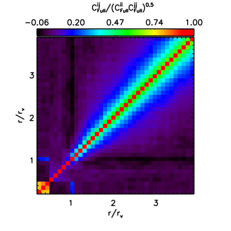
The top-right panel of Fig. 4 shows an example of the full covariance matrix. The correlation between neighbouring bins can be at the 50% level at $r>r_{\rm v}$, dropping to the 10% to 20% level when radial bins are more than 0.2$r_{\rm v}$ apart. This suggests that the overlap of volume among different voids is not so strong in our sample.

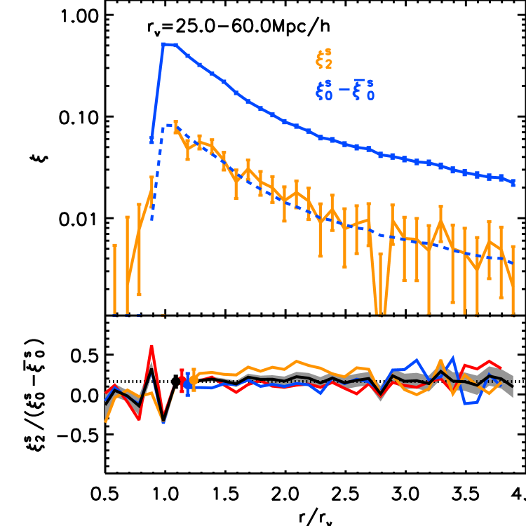
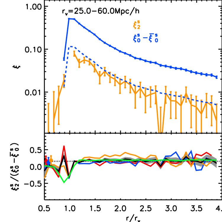
The bottom-left panel of Fig. 4 shows the corresponding quadrupole and monopole from averaging over voids viewed along all the three major axes of the simulation box. While the amplitude of the quadrupole remains very small at all scales, the ratio between the quadrupole and monopole is very nearly independent of radius for $r>r_{\rm v}$. The measurement inevitably becomes noisier at smaller radii, as there are fewer haloes there, but in general the ratio drops in this regime and in some cases becomes negative. This is expected as the impact of velocity dispersion is dominant over the linear streaming motion, causing the correlation function to be less flattened or even to become elongated. The linear model clearly fails at $r<r_{\rm v}$; in the following, we perform fitting to the measurement using two different models at $r>r_{\rm v}$ and $r>0.5r_{\rm v}$ respectively.

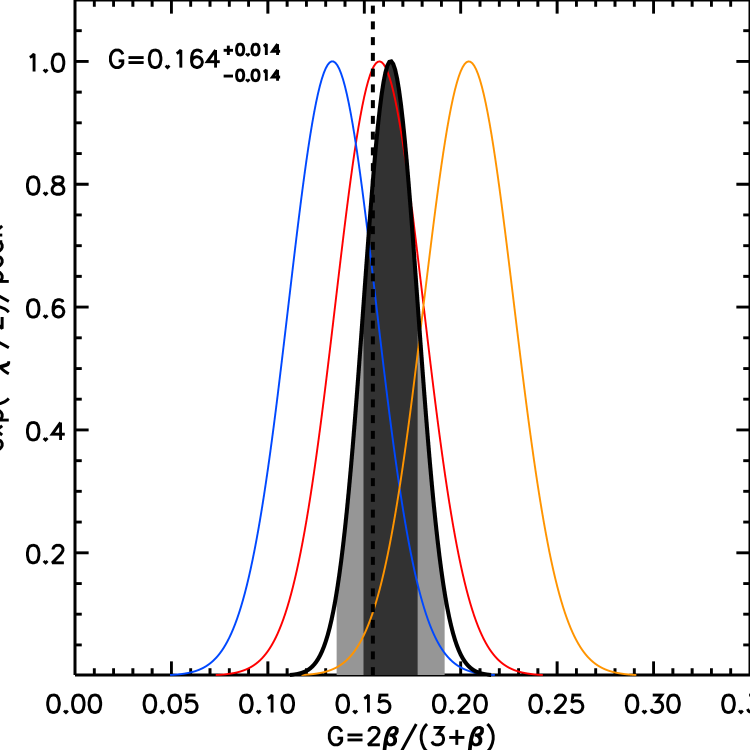
For $r>r_{\rm v}$, we adopt the linear model. We obtain a best-fit value for the growth factor $G$, as indicated by the red, blue and orange dots with error bars for a volume of 1(Gpc/$h$)³ and the black version is for an effective volume of 3(Gpc/$h$)³. It can be seen that this is unbiased. The precision of the measurement of the growth factor $G$ is about 9% for our effective simulation volume of $3(h^{-1}{\rm Gpc})^{3}$. This translates into a 9% uncertainty in $\beta$.

Figure 6: Likelihoods of the growth parameter $G$ for the measurements of the three sub-samples of voids: $r_{v}=25-30\,h^{-1}{\rm Mpc}$, $r_{v}=30-40\,h^{-1}{\rm Mpc}$ and $r_{v}=40-60\,h^{-1}{\rm Mpc}$ from the left to the right. Top panels are results using the linear model. Bottom panels are results from using the quasi-linear model with two free parameters $[\sigma_{0},G]$, where $\sigma_{0}$ is the amplitudes of the velocity dispersion profile taken to follow an error function form, i.e. $\sigma_{\rm v}(r)=\sigma_{0}{\rm erf}(r/r_{\rm v})$. The $\sigma_{0}$ parameters are marginalised.

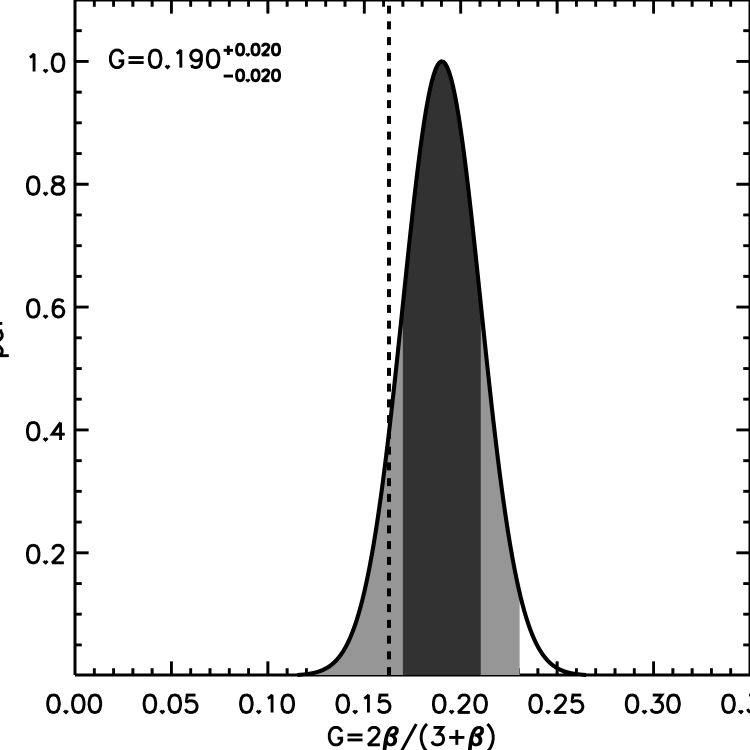
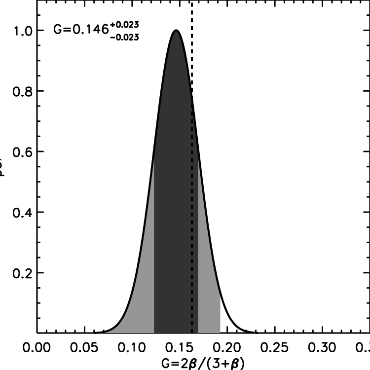
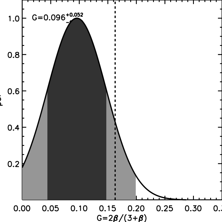
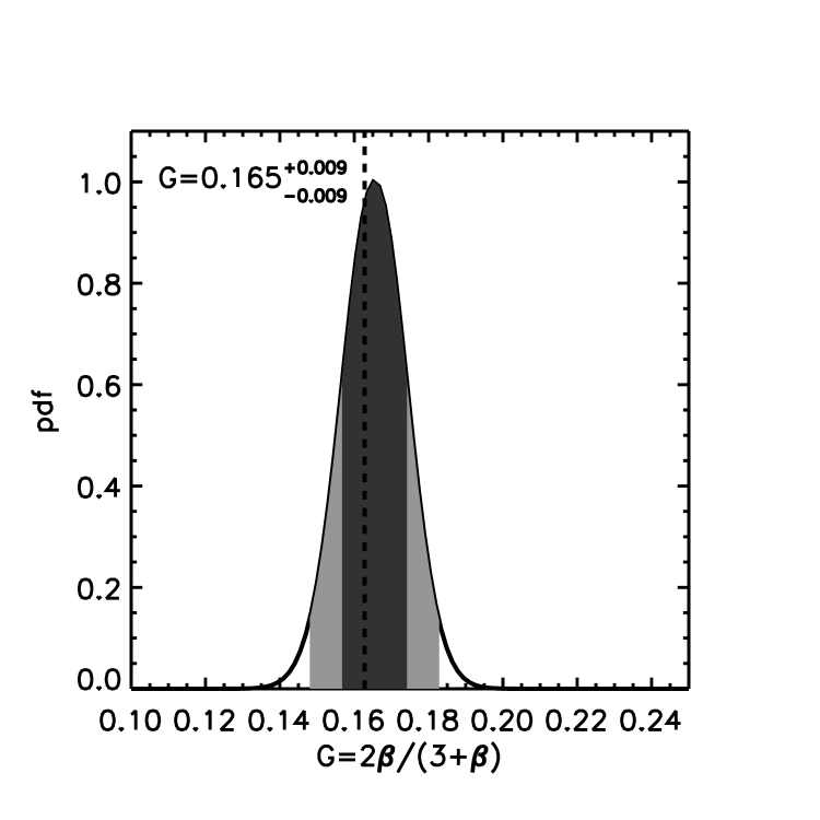
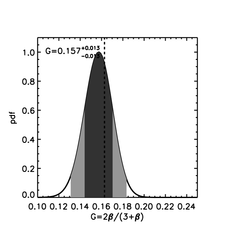
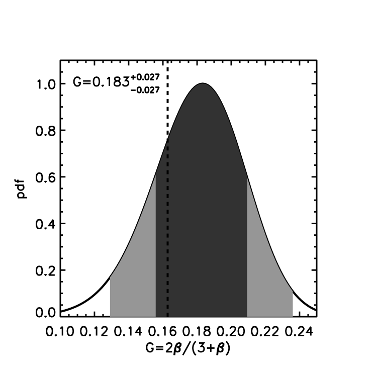
Since large voids have larger volume and contain more haloes than small ones, they are expected to have higher signal-to-noise per void. We try weighting voids according to their volume in our analysis, finding that the error budget is reduced by $\approx 10\%$ and the peak of the likelihood is shifted to the left by approximately 8%, which brings in better agreement (within 1$\sigma$) with the fiducial value. The precision of the measurement of the growth factor $G$ is about 8% for the volume of 3(Gpc/$h$)³, as shown by the likelihood function computed from $\exp({-\chi^{2}/2})$ on the bottom-left panel of Fig. 4. This also translates into a 9% constraint for $\beta$ as the central value is slightly lower than the case without weighting.

We find that including voids with radii smaller than 25$\,h^{-1}{\rm Mpc}$ does not help to reduce the error significantly, given that the number of voids is significantly increased, but inclusion of these voids introduces a bias in the best-fit value of $\beta$. This is possibly because small voids are more likely to be sub-voids: these essentially sample part of the volume that has already been used, thus adding no more information other than introducing covariance. In particular, we find that these small voids are more likely to be void-in-cloud objects, i.e. voids that live in overdense environments. Such systems tend to have over-compensated profiles, which are more complicated to model, with non-linear effects associated with the over-compensated wall. Indeed, we have found that there is a scale-dependent ratio between the real-space void-halo cross-correlation $\xi_{\rm vh}$ and the void-mass cross-correlation $\xi_{\rm vm}$ when smaller voids are included. It may also be that, for such small voids, neglect of their correlated velocity field is not justified in the way that applies for the larger voids (see the discussion in Section 4.1).

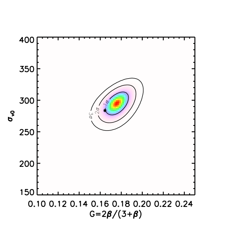
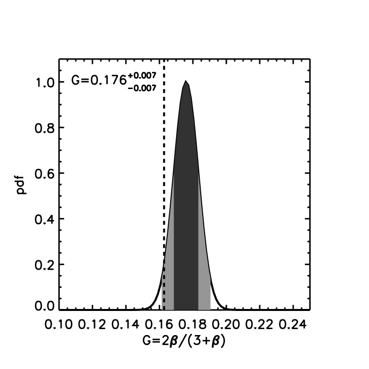
For $r>0.5r_{\rm v}$, we fit our measurement with the quasi-linear model shown in Eq. (9). Void profiles are taken from the measured monopoles and the radial velocity profiles are inferred from linear theory using the monopoles. Motivated by the simulation results shown in Figs 1-3, we adopt an error function form for the velocity dispersion profile and allow its amplitude to vary, i.e. $\sigma_{\rm v}(r)=\sigma_{0}\,{\rm erf}(r/r_{v})$, where $\sigma_{0}$ is a free parameter. We compute $\chi^{2}$s in the [G, $\sigma_{0}$] 2D parameter space, and the resulting joint constraints on $\sigma_{0}$ and $G$ are shown on the top-left panel of Fig. 5. The fiducial values are found to be consistent with the measurement within $1\sigma$. There is, as expected, a degree of correlation between $G$ and $\sigma_{0}$, so that the conditional error on $G$ at fixed $\sigma_{0}$ is smaller than the true error on $G$, marginalized over $\sigma_{0}$; this yields the constraint on $G$ shown in the top-right panel of Fig. 5. However, because we are now able to include data at smaller $r$, the error budget is a factor of two smaller than when using the linear model with $r>r_{\rm v}$. Therefore, our precision on $\beta$ in this case is $\approx 5\%$. The green curve at the bottom panel of the figure shows our best-fit model, which matches the data very well throughout the range of scales shown. The impact of velocity dispersion is indeed only important at $r<r_{\rm v}$. So $\sigma_{0}$ is constrained mainly by small scales, while $\beta$ is sensitive to the clustering throughout the whole range of scales; this explains why $\sigma_{0}$ and $\beta$ are not completely degenerate. With this model, we have again found that including smaller voids does not help to tighten the constraint for the growth. However, including these voids can have the effect of biasing the recovered growth rate above the fiducial value, by as much as 20%. We therefore recommend that practical analyses should be restricted to voids with $r_{\rm v}>25\,h^{-1}{\rm Mpc}$.

To check that the success of our measurements for the growth parameter is robust, we split the void population into three sub-samples covering different ranges of void radius, i.e. $r_{v}=25-30\,h^{-1}{\rm Mpc}$, $r_{v}=30-40\,h^{-1}{\rm Mpc}$ and $r_{v}=40-60\,h^{-1}{\rm Mpc}$. We then repeat the analysis for each with both the linear model and the quasi-linear model. The likelihoods for the growth parameter $G$ (after marginalising over the velocity dispersion parameter for the quasi-linear case) are shown in Fig. 6. All results are consistent with the fiducial values within $2\sigma$ and the agreement for the results using the quasi-linear model are slightly better. Note that the best-fit values of $\sigma_{0}$ are also different for each of the three sub-samples. This explains why the overall agreement here is better than when fitting the whole sample assuming a universal value of $\sigma_{0}$ (Fig. 5). Thus, this analysis of sub-samples not only verifies the success of our method for measuring the growth parameter, but also shows that it is better to split the void sample into sub-samples of different radius when including a velocity dispersion in the fitting.

Note that our measurement requires no prior knowledge of the void profile, and works with quantities that we can directly measure from the data. The success of the measurement is guaranteed by the good agreement between the recovered monopole from the redshift space correlation function with the true answer, as shown by the overlap between the red dots and the red dashed curves in the bottom-left panels of Figs 1, 2 and 3. The measurement of these moments for individual voids is very noisy as each void has its intrinsic configuration, but by averaging measurements over all voids in our sample, we are able to beat down the noise and recover the monopole and quadrupoles without any obvious bias (e.g. bottom-left panel of Fig. 4). We have also tested that the best-fit results remains unchanged when we bin our voids in groups of 10 or 20, conduct the measurement for each void composite and take the average.

The simplicity of the linear modelling of void-galaxy cross-correlations contrasts with the modelling of the redshift-space galaxy autocorrelation function, which becomes difficult even at relatively large scales. For example, recent measurements of the growth rate using the galaxy autocorrelation function (Samushia et al., 2014; Howlett et al., 2015) restricted their analyses to scales greater than 24$\,h^{-1}{\rm Mpc}$ and 25$\,h^{-1}{\rm Mpc}$ respectively. This is the same as the minimal void radius in our analysis, but the autocorrelation analysis requires careful modelling of velocity dispersion even to reach these scales, whereas we have seen that it is unimportant for voids. Adding the dispersion term in the quasi-linear model allows us to use information down to the much smaller scales of $r=0.5r_{\rm v}$, or $12\,h^{-1}{\rm Mpc}$ for the void sample where the results are robust.

4.3 Comparison to Hamaus et al.

During the preparation of this manuscript, two papers on the same topic were released (Hamaus et al., 2015, 2016) [see also Mao et al. (2016) and Shoji & Lee (2012) where the impact of redshift-space distortion on void ellipticity is studied in the latter]. Our work is distinct in terms of void definition, methodology of measuring the growth as well as the prior assumptions in the model fitting. Hamaus et al. (2015) and Hamaus et al. (2016) use vide (Sutter et al., 2015), which is based on the watershed algorithm of zobov (Neyrinck, 2008) for HOD galaxies. We employ the spherical underdensity void-finding algorithm for haloes (Padilla et al., 2005; Cai et al., 2015). Hamaus et al. (2015) and Hamaus et al. (2016) assumed a 4-parameter model for the void profile (which largely depends on the void finding algorithm) and marginalised over this model. In our methodology, no prior assumption about the void profiles is needed, as we have shown that we can measure the void profile from the monopole of the data. Our analysis pipeline is in principle applicable to voids defined from any void-finding algorithm. Hamaus et al. (2015) assumed a Lorentzian distribution for the velocity dispersion, and fixed the width of the Lorentzian function (using the best fit value from their simulations) prior to their MCMC fitting. In our linear analysis, no model assumption for the velocity is needed; and in our quasi-linear analysis, we only assume a functional form for the dispersion profile without fixing anything further. Hamaus et al. (2015) and Hamaus et al. (2016) have to bin their voids before fitting, which may come from the restriction that they have to assume a model for the void profile, and the model may not be able to describe individual profile. Our analysis is flexible as we have shown that binning our voids in sets of 10, 20 or not binning at all yields the same results. Hamaus et al. (2015) included the distance distortion parameter related to the AP test for their fitting. We restrict our analysis to a single free parameter of the growth for the purpose of understanding how the configuration of voids are affected by peculiar velocity.

Perhaps more importantly, the results from Hamaus et al. (2015) for the growth appear to be dominated by systematics and are strongly biased from their fiducial values , whereas our measurement for the growth displays no significant bias within our chosen range of void sizes. We suspect that a possible reason for the bias in the results of Hamaus et al. (2015) is that they have used all data including the very interior of voids and in some cases they have used voids with radii smaller than 10$\,h^{-1}{\rm Mpc}$. We have excluded this region ($r<0.5r_{\rm v}$) from our fitting and restrict our analysis to using voids with $r_{\rm v}>25\,h^{-1}{\rm Mpc}$. It is likely that for very small voids, or at void centres, structure formation is highly non-linear so that the quasi-linear model does not work there.

Finally, our results are also noticeably different from those of Hamaus et al. (2016) for the best constraint on the growth parameter. Using voids from a volume of $3.5(h^{-1}{\rm Gpc})^{3}$ from the SDSS DR11 CMASS galaxy sample, they report constraints on $\beta$ at the 20% level . With a similar volume of $3(h^{-1}{\rm Gpc})^{3}$ from simulation, our best constraint on $\beta$ is a few times tighter, i.e. at the $5\%$ level.

5 conclusions and discussion

We have derived models for the void-halo or void-galaxy correlation function in redshift space as well as their Fourier space versions. We show that the linear-theory void-halo correlation function contains only monopole and quadrupole terms, which allows us to write down an estimator for the fluctuation growth rate based on the ratio of quadrupole and monopole. We then test the estimator for voids found using halo density fields from numerical simulation. We are able to extract the monopole from the correlation function in an unbiased fashion at all scales of interest, including the interior of voids. No prior knowledge of the void profile is needed, as it can be measured from the data. This approach is to be contrasted with the work of Ceccarelli et al. (2013) and Paz et al. (2013), who used SDSS voids to estimate the mean radial velocity profile for voids, whereas we are able to obtain this from linear theory.

The ratio between monopole and quadrupole provides an unbiased estimates for the growth parameter $\beta=f/b$ at $r>r_{\rm v}$. For an effective volume of $3(h^{-1}{\rm Gpc})^{3}$, $\beta$ is constrained in this way with 9% precision. Extending the model to allow for a dispersion of random velocities allows us to apply the quasi-linear model at smaller scales $r>0.5r_{\rm v}$ and tighten the constraint for $\beta$ by a factor of two. In principle, our estimator is applicable to any void finding algorithm, since we have made no assumption beyond linear theory and have no specific requirement for the void population. We find that including scales below $r<0.5r_{\rm v}$ can bias the results. This is probably because the centres of voids are evolving in a highly non-linear fashion and so it is beyond the description of the quasi-linear model. We have noted that this lack of bias contrasts with the results of the recent paper by Hamaus et al. (2015), and we have highlighted some methodological differences between our studies that may account for this rather different outcome.

Our models allow us to understand the complex distortion pattern of voids generated by peculiar velocities. We find that voids may appear elongated or flattened along the line of sight at different radii: this can be explained by the competing amplitudes of the local density, radial velocity profiles and their gradients, with the latter two being determined by the cumulative density profile of voids in linear theory. Velocity dispersion causes a slight elongation along the LOS for the correlation function, which counters the flattening effect caused by the streaming motion in the interior of the void and sometimes reverses it, causing the sign of the quadrupole to flip. However, the effect of a random velocity dispersion is usually negligible outside the void radius. Thus the dispersion patten for voids is complex, and the key element that governs the void distortion pattern at $r>r_{\rm v}$ is mostly the void profile. In light of this, the distortion pattern for voids-in-clouds and voids-in-voids are expected to be different. The picture will change when there is strong non-linearity, but we have demonstrated that for large voids with radii greater than 25$\,h^{-1}{\rm Mpc}$, the quasi-linear model works very well.

The distortion patterns of voids in redshift space is more complex and is distinct from redshift-space distortions in overdensities. For overdensities, infall motions cause flattening on large scales and random velocity dispersions induce elongation along the line of sight on small scales.

Our study implies that Alcock-Paczynski (AP) measurements using voids will be affected by peculiar velocity distortions in a complex manner. Assuming the correct cosmology, the dimension of voids along the LOS may appear greater or smaller than that in the transverse direction. It depends on the void population, and for the same void population there is also a radial dependence. Ultimately, knowing the void profile is the key to understanding the impact of peculiar velocities on the apparent axial ratios of voids and on the resulting AP measurement. Fortunately, we have shown that the redshift-space void profile can be successfully extracted from the void-halo correlation function. This may provide the key information to correct for the AP measurement using voids.

A striking conclusion of this study is that the void-galaxy correlation function may be able to provide a high precision on the growth rate (5% for $\beta$ for a volume of $3(h^{-1}{\rm Gpc})^{3}$, comparable to that obtained from using the LRG autocorrelation function – e.g. Samushia et al. (2014) found a precision of 10% from a volume of $2(h^{-1}{\rm Gpc})^{3}$. This success depends on the applicability of the quasi-linear model at small scales $r\approx 12\,h^{-1}{\rm Mpc}$; this is easier to achieve using voids, as the signal from extreme overdensities is then removed, and these are hardest to model. Admittedly, adding the AP test parameter may degrade the constraining power for the growth, but perhaps only very mildly [see for example, (Hamaus et al., 2016)]. We leave this investigation for a future work. The next step will be to see if these virtues are maintained when using mock data that accurately match real galaxy catalogues. If this is indeed the case, then we will have not only a tool for assessing the robustness of growth-rate measurements, but also a unique probe of deviations from standard Einstein gravity, which are expected to reveal themselves most strongly in low-density environments.

References

- Alcock & Paczynski (1979) Alcock, C., & Paczynski, B. 1979, Nature, 281, 358
- Barreira et al. (2015) Barreira A., Li B., Jennings E., Merten J., King L., Baugh C. M., Pascoli S., 2015, MNRAS, 454, 4085
- Beutler et al. (2012) Beutler F., Blake C., Colless M., Jones D. H., Staveley-Smith L., Poole G. B., Campbell L., Parker Q., Saunders W., Watson F., 2012, MNRAS, 423, 3430
- Blake et al. (2012) Blake C., Brough S., Colless M., Contreras C., Couch W., Croom S., Croton D., Davis T. M., et al. 2012, MNRAS, 425, 405
- Bos et al. (2012) Bos E. G., van de Weygaert R., Dolag K., Pettorino V., 2012, MNRAS, 426, 440
- Cai et al. (2014a) Cai Y.-C., Li B., Cole S., Frenk C. S., Neyrinck M., 2014, MNRAS, 439, 2978
- Cai et al. (2014b) Cai Y.-C., Neyrinck M. C., Szapudi I., Cole S., Frenk C. S., 2014, ApJ, 786, 110
- Cai et al. (2015) Cai Y.-C., Padilla N., Li B., 2015, MNRAS, 451, 1036
- Ceccarelli et al. (2013) Ceccarelli L., Paz D., Lares M., Padilla N., Lambas D. G., 2013, MNRAS, 434, 1435
- Chan et al. (2014) Chan, K. C., Hamaus, N., & Desjacques, V. 2014, Phys. Rev. D, 90, 103521
- Clampitt et al. (2013) Clampitt J., Cai Y.-C., Li B., 2013, MNRAS, 431, 749
- Clampitt & Jain (2015) Clampitt J., Jain B., 2015, MNRAS, 454, 3357
- Croft et al. (1999) Croft, R. A. C., Dalton, G. B., & Efstathiou, G. 1999, MNRAS, 305, 547
- Cole et al. (1994) Cole S., Fisher K. B., Weinberg D. H., 1994, MNRAS, 267, 785
- Cole et al. (1995) Cole S., Fisher K. B., Weinberg D. H., 1995, MNRAS, 275, 515
- de la Torre & Guzzo (2012) de la Torre S., Guzzo L., 2012, MNRAS, 427, 327
- de la Torre et al. (2013) de la Torre S., Guzzo L., Peacock J. A., Branchini E., Iovino A., Granett B. R., Abbas U., Adami C., et al. 2013, A&A, 557, A54
- Fisher (1995) Fisher K. B., 1995, ApJ, 448, 494
- Fisher et al. (1994a) Fisher K. B., Davis M., Strauss M. A., Yahil A., Huchra J., 1994a, MNRAS, 266, 50
- Fisher et al. (1994b) Fisher K. B., Davis M., Strauss M. A., Yahil A., Huchra J. P., 1994b, MNRAS, 267, 927
- Gil-Marín et al. (2012) Gil-Marín H., Wagner C., Verde L., Porciani C., Jimenez R., 2012, JCAP, 11, 29
- Granett et al. (2008) Granett B. R., Neyrinck M. C., Szapudi I., 2008, ApJ, 683, L99
- Gruen et al. (2016) Gruen D., Friedrich O., Amara A., Bacon D., Bonnett C., Hartley W., Jain B., Jarvis M., et al. 2016, MNRAS, 455, 3367
- Hamaus et al. (2014) Hamaus, N., Wandelt, B. D., Sutter, P. M., Lavaux, G., & Warren, M. S. 2014, Physical Review Letters, 112, 041304
- Hamaus et al. (2015) Hamaus, N., Sutter, P. M., Lavaux, G., & Wandelt, B. D. 2015, JCAP, 11, 036
- Hamaus et al. (2016) Hamaus, N., Pisani, A., Sutter, P. M., et al. 2016, arXiv:1602.01784
- Hamilton (1992) Hamilton A. J. S., 1992, ApJ, 385, L5
- Hamilton (1998) Hamilton A. J. S., 1998, in Hamilton D., ed., The Evolving Universe Vol. 231 of Astrophysics and Space Science Library, Linear Redshift Distortions: a Review. p. 185
- Higuchi et al. (2013) Higuchi Y., Oguri M., Hamana T., 2013, MNRAS, 432, 1021
- Howlett et al. (2015) Howlett C., Ross A. J., Samushia L., Percival W. J., Manera M., 2015, MNRAS, 449, 848
- Jennings et al. (2011) Jennings E., Baugh C. M., Pascoli S., 2011, MNRAS, 410, 2081
- Kaiser (1987) Kaiser N., 1987, MNRAS, 227, 1
- Kitaura et al. (2016) Kitaura, F.-S., Chuang, C.-H., Liang, Y., et al. 2016, Physical Review Letters, 116, 171301
- Krause et al. (2013) Krause E., Chang T.-C., Doré O., Umetsu K., 2013, ApJ, 762, L20
- Lam et al. (2015) Lam, T. Y., Clampitt, J., Cai, Y.-C., & Li, B. 2015, MNRAS, 450, 3319
- Lavaux & Wandelt (2012) Lavaux G., Wandelt B. D., 2012, ApJ, 754, 109
- Lee & Park (2009) Lee, J., & Park, D. 2009, ApJ, 696, L10
- Li et al. (2013) Li B., Hellwing W. A., Koyama K., Zhao G.-B., Jennings E., Baugh C. M., 2013, MNRAS, 428, 743
- Liang et al. (2016) Liang, Y., Zhao, C., Chuang, C.-H., Kitaura, F.-S., & Tao, C. 2016, MNRAS, 459, 4020
- Mao et al. (2016) Mao, Q., Berlind, A. A., Scherrer, R. J., et al. 2016, arXiv:1602.06306
- Massara et al. (2015) Massara, E., Villaescusa-Navarro, F., Viel, M., & Sutter, P. M. 2015, JCAP, 11, 018
- Matsubara (2008) Matsubara T., 2008, Phys. Rev. D, 78, 083519
- Mo et al. (1993) Mo, H. J., Peacock, J. A., & Xia, X. Y. 1993, MNRAS, 260, 121
- Neyrinck (2008) Neyrinck, M. C. 2008, MNRAS, 386, 2101
- Okumura et al. (2015) Okumura T., Hand N., Seljak U., Vlah Z., Desjacques V., 2015, Phys. Rev. D, 92, 103516
- Okumura et al. (2016) Okumura T., Hikage C., Totani T., Tonegawa M., Okada H., Glazebrook K., Blake C., Ferreira P. G., et al. 2016, PASJ, 68, 38
- Okumura et al. (2012) Okumura T., Seljak U., McDonald P., Desjacques V., 2012, JCAP, 2, 10
- Padilla et al. (2005) Padilla N. D., Ceccarelli L., Lambas D., 2005, MNRAS, 363, 977
- Paz et al. (2013) Paz D., Lares M., Ceccarelli L., Padilla N., Lambas D. G., 2013, MNRAS, 436, 3480
- Peacock et al. (2001) Peacock J. A., Cole S., Norberg P., Baugh C. M., Bland-Hawthorn J., Bridges T., Cannon R. D., Colless M., et al. 2001, Nature, 410, 169
- Peebles (1993) Peebles P. J. E., 1993, Principles of Physical Cosmology. Princeton University Press
- Percival & White (2009) Percival W. J., White M., 2009, MNRAS, 393, 297
- Pollina et al. (2016) Pollina, G., Baldi, M., Marulli, F., & Moscardini, L. 2016, MNRAS, 455, 3075
- Reid et al. (2012) Reid B. A., Samushia L., White M., Percival W. J., Manera M., Padmanabhan N., Ross A. J., Sánchez A. G., et al. 2012, MNRAS, 426, 2719
- Reid et al. (2014) Reid B. A., Seo H.-J., Leauthaud A., Tinker J. L., White M., 2014, MNRAS, 444, 476
- Sachs & Wolfe (1967) Sachs, R. K., & Wolfe, A. M. 1967, ApJ, 147, 73
- Samushia et al. (2014) Samushia L., Reid B. A., White M., Percival W. J., Cuesta A. J., Zhao G.-B., Ross A. J., Manera M., et al. 2014, MNRAS, 439, 3504
- Scoccimarro (2004) Scoccimarro R., 2004, Phys. Rev. D, 70, 083007
- Seljak & McDonald (2011) Seljak U., McDonald P., 2011, JCAP, 11, 39
- Sheth & van de Weygaert (2004) Sheth R. K., van de Weygaert R., 2004, MNRAS, 350, 517
- Shoji & Lee (2012) Shoji, M., & Lee, J. 2012, arXiv:1203.0869
- Sutter et al. (2014) Sutter P. M., Pisani A., Wandelt B. D., Weinberg D. H., 2014, MNRAS, 443, 2983
- Sutter et al. (2015) Sutter, P. M., Lavaux, G., Hamaus, N., et al. 2015, Astronomy and Computing, 9, 1
- Taruya et al. (2010) Taruya A., Nishimichi T., Saito S., 2010, Phys. Rev. D, 82, 063522
- Taruya et al. (2009) Taruya A., Nishimichi T., Saito S., Hiramatsu T., 2009, Phys. Rev. D, 80, 123503
- Valageas et al. (2013) Valageas P., Nishimichi T., Taruya A., 2013, Phys. Rev. D, 87, 083522
- Yang et al. (2015) Yang L. F., Neyrinck M. C., Aragón-Calvo M. A., Falck B., Silk J., 2015, MNRAS, 451, 3606
- Zivick et al. (2015) Zivick P., Sutter P. M., Wandelt B. D., Li B., Lam T. Y., 2015, MNRAS, 451, 4215
- Zu & Weinberg (2013) Zu Y., Weinberg D. H., 2013, MNRAS, 431, 3319