Turing learning: a metric-free approach to inferring behavior and its application to swarms

Abstract

We propose Turing Learning, a novel system identification method for inferring the behavior of natural or artificial systems. Turing Learning simultaneously optimizes two populations of computer programs, one representing models of the behavior of the system under investigation, and the other representing classifiers. By observing the behavior of the system as well as the behaviors produced by the models, two sets of data samples are obtained. The classifiers are rewarded for discriminating between these two sets, that is, for correctly categorizing data samples as either genuine or counterfeit. Conversely, the models are rewarded for ‘tricking’ the classifiers into categorizing their data samples as genuine. Unlike other methods for system identification, Turing Learning does not require predefined metrics to quantify the difference between the system and its models. We present two case studies with swarms of simulated robots and prove that the underlying behaviors cannot be inferred by a metric-based system identification method. By contrast, Turing Learning infers the behaviors with high accuracy. It also produces a useful by-product—the classifiers—that can be used to detect abnormal behavior in the swarm. Moreover, we show that Turing Learning also successfully infers the behavior of physical robot swarms. The results show that collective behaviors can be directly inferred from motion trajectories of individuals in the swarm, which may have significant implications for the study of animal collectives. Furthermore, Turing Learning could prove useful whenever a behavior is not easily characterizable using metrics, making it suitable for a wide range of applications.
Keywords: system identification; Turing test; collective behavior; swarm robotics; coevolution; machine learning

1 Introduction

System identification is the process of modeling natural or artificial systems through observed data. It has drawn a large interest among researchers for decades (Ljung, 2010; Billings, 2013). A limitation of current system identification methods is that they rely on predefined metrics, such as the sum of square errors, to measure the difference between the output of the models and that of the system under investigation. Model optimization then proceeds by minimizing the measured differences. However, for complex systems, defining a metric can be non-trivial and case-dependent. It may require prior information about the systems. Moreover, an unsuitable metric may not distinguish well between good and bad models, or even bias the identification process. This paper overcomes these problems by introducing a system identification method that does not rely on predefined metrics.

A promising application of such a metric-free method is the identification of collective behaviors, which are emergent behaviors that arise from the interactions of numerous simple individuals (Camazine et al., 2003). Inferring collective behaviors is particularly challenging, as the individuals not only interact with the environment but also with each other. Typically, their motion appears stochastic and is hard to predict (Helbing and Johansson, 2011). For instance, given a swarm of simulated fish, one would have to evaluate how close its behavior is to that of a real fish swarm, or how close the individual behavior of a simulated fish is to that of a real fish. Characterizing the behavior at the level of the swarm is difficult (Harvey et al., 2015). Such a metric may require domain-specific knowledge; moreover, it may not be able to discriminate among distinct individual behaviors that lead to similar collective dynamics (Weitz et al., 2012). Characterizing the behavior at the level of individuals is also difficult, as even the same individual fish in the swarm is likely to exhibit a different trajectory every time it is being looked at.

In this paper, we propose Turing Learning, a novel system identification method that allows a machine to autonomously infer the behavior of a natural or artificial system. Turing Learning simultaneously optimizes two populations of computer programs, one representing models of the behavior, the other representing classifiers. The purpose of the models is to imitate the behavior of the system under investigation. The purpose of the classifiers is to discriminate between the behaviors produced by the system and any of the models. In Turing Learning, all behaviors are observed for a period of time. This generates two sets of data samples. The first set consists of genuine data samples, which originate from the system. The second set consists of counterfeit data samples, which originate from the models. The classifiers are rewarded for discriminating between samples of these two sets: Ideally, they should recognize any data sample from the system as genuine, and any data sample from the models as counterfeit. Conversely, the models are rewarded for their ability to ‘trick’ the classifiers into categorizing their data samples as genuine.

Turing Learning does not rely on predefined metrics for measuring how close the models reproduce the behavior of the system under investigation; rather, the metrics (classifiers) are produced as a by-product of the identification process. The method is inspired by the Turing test (Turing, 1950; Saygin et al., 2000; Harnad, 2000), which machines can pass if behaving indistinguishably from humans. Similarly, the models could pass the tests by the classifiers if behaving indistinguishably from the system under investigation. We hence call our method Turing Learning.

In the following, we examine the ability of Turing Learning to infer the behavioral rules of a swarm of mobile agents. The agents are either simulated or physical robots. They execute known behavioral rules. This allows us to compare the inferred models to the ground truth. To obtain the data samples, we record the motion trajectories of all the agents. In addition, we record the motion trajectories of an agent replica, which is mixed into the group of agents. The replica executes the rules defined by the models—one at a time. As will be shown, by observing the motion trajectories of agents and of the agent replica, Turing Learning automatically infers the behavioral rules of the agents. The behavioral rules examined here relate to two canonical problems in swarm robotics: self-organized aggregation (Gauci et al., 2014c), and object clustering (Gauci et al., 2014b). They are reactive; in other words, each agent maps its inputs (sensor readings) directly onto the outputs (actions). The problem of inferring the mapping is challenging, as the inputs are not known. Instead, Turing Learning has to infer the mapping indirectly, from the observed motion trajectories of the agents and of the replica.

We originally presented the basic idea of Turing Learning, along with preliminary simulations, in (Li et al., 2013, 2014). This paper extends our prior work as follows:

• It presents an algorithmic description of Turing Learning;

• It shows that Turing Learning outperforms a metric-based system identification method in terms of model accuracy;

• It proves that the metric-based method is fundamentally flawed, as the globally optimal solution differs from the solution that should be inferred;

• It demonstrates, to the best of our knowledge for the first time, that system identification can infer the behavior of swarms of physical robots;

• It examines in detail the usefulness of the classifiers;

• It examines through simulation how Turing Learning can simultaneously infer the agent’s brain (controller) and an aspect of its morphology that determines the agent’s field of view;

• It demonstrates through simulation that Turing Learning can infer the behavior even if the agent’s control system structure is unknown.

This paper is organized as follows. Section 2 discusses related work. Section 3 describes Turing Learning and the general methodology of the two case studies. Section 4 investigates the ability of Turing Learning to infer two behaviors of swarms of simulated robots. It also presents a mathematical analysis, proving that these behaviors cannot be inferred by a metric-based system identification method. Section 5 presents a real-world validation of Turing Learning with a swarm of physical robots. Section 6 concludes the paper.

2 Related work

This section is organized as follows. First, we outline our previous work on Turing Learning, and review a similar line of research, which has appeared since its publication. As the Turing Learning implementation uses coevolutionary algorithms, we then overview work using coevolutionary algorithms (but with predefined metrics), as well as work on the evolution of physical systems. Finally, works using replicas in ethological studies are presented.

Turing Learning is a system identification method that simultaneously optimizes a population of models and a population of classifiers. The objective for the models is to be indistinguishable from the system under investigation. The objective for the classifiers is to distinguish between the models and the system. The idea of Turing Learning was first proposed in (Li et al., 2013); this work presented a coevolutionary approach for inferring the behavioral rules of a single agent. The agent moved in a simulated, one-dimensional environment. Classifiers were rewarded for distinguishing between the models and the agent. In addition, they were able to control the stimulus that influenced the behavior of the agent. This allowed the classifiers to interact with the agent during the learning process. Turing Learning was subsequently investigated with swarms of simulated robots (Li et al., 2014).

Goodfellow et al. (2014) proposed generative adversarial nets (GANs). GANs, while independently invented, are essentially based on the same idea as Turing Learning. The authors used GANs to train models for generating counterfeit images that resemble real images, for example, from the Toronto Face Database (for further examples, see (Radford et al., 2016)). They simultaneously optimized a generative model (producing counterfeit images) and a discriminative model that estimates the probability of an image to be real. The optimization was done using a stochastic gradient descent method.

In a work reported in (Herbert-Read et al., 2015), humans were asked to discriminate between the collective motion of real and simulated fish. The authors reported that the humans could do so even though the data from the model were consistent with the real data according to predefined metrics. Their results “highlight a limitation of fitting detailed models to real-world data”. They argued that “observational tests […] could be used to cross-validate models” (see also Harel (2005)). This is in line with Turing Learning. Our method, however, automatically generates both the models and the classifiers, and thus does not require human observers.

While Turing Learning can in principle be used with any optimization algorithm, our implementation relies on coevolutionary algorithms. Metric-based coevolutionary algorithms have already proven effective for system identification (Bongard and Lipson, 2004a; Bongard and Lipson, 2004b; Bongard and Lipson, 2005, 2007; Koos et al., 2009; Mirmomeni and Punch, 2011; Le Ly and Lipson, 2014). A range of work has been performed on simulated agents. Bongard and Lipson (2004a) proposed the estimation-exploration algorithm, a nonlinear system identification method to coevolve inputs and models in a way that minimizes the number of inputs to be tested on the system. In each generation, the input (test) that led, in simulation, to the highest disagreement between the models’ predicted outputs was carried out on the real system. The models’ predictions were then compared with the actual output of the system. The method was applied to evolve morphological parameters of a simulated quadrupedal robot after it had undergone physical damage. In a later work (Bongard and Lipson, 2004b), the authors reported that “in many cases the simulated robot would exhibit wildly different behaviors even when it very closely approximated the damaged ‘physical’ robot. This result is not surprising due to the fact that the robot is a highly coupled, non-linear system: Thus similar initial conditions […] are expected to rapidly diverge in behavior over time”. The authors addressed this problem by using a more refined comparison metric reported in (Bongard and Lipson, 2004b). In (Koos et al., 2009), an algorithm which also coevolves models and inputs (tests) was presented to model a simulated quadrotor and improve the control quality. The tests were selected based on multiple criteria: to provide disagreement between models as in (Bongard and Lipson, 2004a), and to evaluate the control quality in a given task. Models were then refined by comparing the predicted trajectories with those of the real system. In these works, predefined metrics were critical for evaluating the performance of models. Moreover, the algorithms are not applicable to the scenarios we consider here, as the system’s inputs are assumed to be unknown (the same would typically also be the case for biological systems).

Some studies also investigated the implementation of evolution directly in physical environments, on either a single robot (Floreano and Mondada, 1996; Zykov et al., 2004; Bongard et al., 2006; Koos et al., 2013; Cully et al., 2015) or multiple robots (Watson et al., 2002; O’Dowd et al., 2014; Heinerman et al., 2015). In (Bongard et al., 2006), a four-legged robot was built to study how it can infer its own morphology through a process of continuous self-modeling. The robot ran a coevolutionary algorithm on its onboard processor. One population evolved models for the robot’s morphology, while the other evolved actions (inputs) to be conducted on the robot for gauging the quality of these models. Note that this approach required knowledge of the robot’s inputs (sensor data). O’Dowd et al. (2014) presented a distributed approach to coevolve onboard simulators and controllers for a swarm of ten robots. Each robot used its simulators to evolve controllers for performing foraging behavior. The best performing controller was then used to control the physical robot. The foraging performances of the robot and of its neighbors were then compared to inform the evolution of simulators. This physical/embodied evolution helped reduce the reality gap between the simulated and physical environments (Jakobi et al., 1995). In all these approaches, the model optimization was based on predefined metrics (explicit or implicit).

The use of replicas can be found in ethological studies in which researchers use robots that interact with animals (Vaughan et al., 2000; Halloy et al., 2007; Faria et al., 2010; Halloy et al., 2013; Schmickl et al., 2013). Robots can be created and systematically controlled in such a way that they are accepted as conspecifics or heterospecifics by the animals in the group (Krause et al., 2011). For example, in (Faria et al., 2010), a replica fish, which resembled sticklebacks in appearance, was created to investigate two types of interaction: recruitment and leadership. In (Halloy et al., 2007), autonomous robots, which executed a model, were mixed into a group of cockroaches to modulate their decision-making of selecting a shelter. The robots behaved in a similar way to the cockroaches. Although the robots’ appearance was different from that of the cockroaches, the robots released a specific odor such that the cockroaches would perceive them as conspecifics. In these works, the models were manually derived and the robots were only used for model validation. We believe that this robot-animal interaction framework could be enhanced through Turing Learning, which autonomously infers the collective behavior.

3 Methodology

In this section, we present the Turing Learning method and show how it can be applied to two case studies in swarm robotics.

3.1 Turing learning

Turing Learning is a system identification method for inferring the behavior of natural or artificial systems. Turing Learning needs data samples of the behavior—we refer to these data samples as genuine. For example, if the behavior of interest were to shoal like fish, genuine data samples could be trajectory data from fish. If the behavior were to produce paintings in a particular style (e.g., Cubism), genuine data samples could be existing paintings in this style.

Turing Learning simultaneously optimizes two populations of computer programs, one representing models of the behavior, the other representing classifiers. The purpose of the models is to imitate the behavior of the system under investigation. The models are used to produce data samples—we refer to these data samples as counterfeit. There are thus two sets of data samples: one containing genuine data samples, the other containing counterfeit ones. The purpose of the classifiers is to discriminate between these two sets. Given a data sample, the classifiers need to judge where it comes from. Is it genuine, and thus originating from the system under investigation? Or is it counterfeit, and thus originating from a model? This setup is akin of a Turing test; hence the name Turing Learning.

The models and classifiers are competing. The models are rewarded for ‘tricking’ the classifiers into categorizing their data samples as genuine, whereas the classifiers are rewarded for correctly categorizing data samples as either genuine or counterfeit. Turing Learning thus optimizes models for producing behaviors that are seemingly genuine, in other words, indistinguishable from the behavior of interest. This is in contrast to other system identification methods, which optimize models for producing behavior that is as similar as possible to the behavior of interest. The Turing test inspired setup allows for model generation irrespective of whether suitable similarity metrics are known.

The model can be any computer program that can be used to produce data samples. It must however be expressive enough to produce data samples that—from an observer’s perspective—are indistinguishable from those of the system.

The classifier can be any computer program that takes a sequence of data as input and produces a binary output. The classifier must be fed with sufficient information about the behavior of the system. If it has access to only a subset of the behavioral information, any system characteristic not influencing this subset cannot be learned. In principle, classifiers with non-binary outputs (e.g., probabilities or confidence levels) could also be considered.

Algorithm 1 Turing Learning

1:procedure Turing learning

2:     initialize population of $M$ models and population of $N$ classifiers

3:     while termination criterion not met do

4:         for all classifiers $i\in\{1,2,\ldots,N\}$ do

5:              obtain genuine data samples (system, classifier $i$)

6:              for each sample, obtain and store output of classifier $i$

7:              for all models $j\in\{1,2,\ldots,M\}$ do

8:                  obtain counterfeit data samples (model $j$, classifier $i$)

9:                  for each sample, obtain and store output of classifier $i$

10:              end for

11:         end for

12:         reward models ($r_{m}$) for misleading classifiers (classifier outputs)

13:         reward classifiers ($r_{c}$) for making correct judgements (classifier outputs)

14:         improve model and classifier populations based on $r_{m}$ and $r_{c}$

15:     end while

16:end procedure

Algorithm 1 provides a description of Turing Learning. We assume a population of $M>1$ models and a population of $N>1$ classifiers. After an initialization stage, Turing Learning proceeds in an iterative manner until a termination criterion is met.

In each iteration cycle, data samples are obtained from observations of both the system and the models. In the case studies considered here, the classifiers do not influence the sampling process. Therefore, the same set of data samples is provided to all classifiers of an iteration cycle. For simplicity, we assume that each of the $N$ classifiers is provided with $K\geq 1$ data samples for the system and with one data sample for every model.

A model’s quality is determined by its ability of misleading classifiers to judge its data samples as genuine. Let $m_{ij}=1$ if classifier $i$ wrongly classified the data sample of model $j$, and $m_{ij}=0$ otherwise. The quality of model $j$ is then given by:

$${r_{m}(j)}=\frac{1}{N}\sum\limits_{i=1}^{N}m_{ij}.$$ (1)

A classifier’s quality is determined by how well it judges data samples from both the system and its models. The quality of classifier $i$ is given by:

$${r_{c}(i)}=\frac{1}{2}(\mbox{specificity}_{i}+\mbox{sensitivity}_{i}).$$ (2)

The specificity of a classifier (in statistics, also called the true-negative rate) denotes the percentage of genuine data samples that it correctly identified as such. Formally,

$$\mbox{specificity}_{i}=\frac{1}{K}\sum\limits_{k=1}^{K}a_{ik},$$ (3)

where, $a_{ik}=1$ if classifier $i$ correctly classified the $k$th data sample of the system, and $a_{ik}=0$ otherwise.

The sensitivity of a classifier (in statistics, also called the true-positive rate) denotes the percentage of counterfeit data samples that it correctly identified as such. Formally,

$$\mbox{sensitivity}_{i}=\frac{1}{M}\sum\limits_{j=1}^{M}(1-m_{ij}).$$ (4)

Using the solution qualities, $r_{m}$ and $r_{c}$, the model and classifier populations are improved. In principle, any population-based optimization method can be used.

3.2 Case studies

In the following, we examine the ability of Turing Learning to infer the behavioral rules of swarming agents. The swarm is assumed to be homogeneous; it comprises a set of identical agents of known capabilities. The identification task thus reduces to inferring the behavior of a single agent. The agents are robots, either simulated or physical. The agents have inputs (corresponding to sensor reading values) and outputs (corresponding to motor commands). The input and output values are not known. However, the agents are observed and their motion trajectories are recorded. The trajectories are provided to Turing Learning using a reactive control architecture (Brooks, 1991). Evidence indicates that reactive behavioral rules are sufficient to produce a range of complex collective behaviors in both groups of natural and artificial agents (Braitenberg, 1984; Arkin, 1998; Camazine et al., 2003). Note that although reactive architectures are conceptually simple, learning their parameters is not trivial if the agent’s inputs are not available, as is the case in our problem setup. In fact, as shown in Section 4.5, a conventional (metric-based) system identification method fails in this respect.

3.2.1 Agents

Figure 1: An e-puck robot fitted with a black ‘skirt’ and a top marker for motion tracking.

The agents move in a two-dimensional, continuous space. They are differential-wheeled robots. The speed of each wheel can be independently set to $\left[-1,1\right]$, where $-1$ and $1$ correspond to the wheel rotating backwards and forwards, respectively, with maximum speed. Fig. 1 shows the agent platform, the e-puck (Mondada et al., 2009), which is used in the experiments.

Each agent is equipped with a line-of-sight sensor that detects the type of item in front of it. We assume that there are $n$ types (e.g., background, other agent, object (Gauci et al., 2014c, b)). The state of the sensor is denoted by $I\in\{0,1,\ldots,n-1\}$.

Each agent implements a reactive behavior by mapping the input ($I$) onto the outputs, that is, a pair of predefined speeds for the left and right wheels, $(v_{\ell I},v_{rI})$, $v_{\ell I},v_{rI}\in\left[-1,1\right]$. Given $n$ sensor states, the mapping can be represented using $2n$ system parameters, which we denote as:

$$\mathbf{p}=(v_{\ell 0},v_{r0},v_{\ell 1},v_{r1},\cdots,v_{\ell(n-1)},v_{r(n-1)}).$$ (5)

Using $\mathbf{p}$, any reactive behavior for the above agent can be expressed. In the following, we consider two example behaviors in detail.

Aggregation: In this behavior, the sensor is binary, that is, $n=2$. It gives a reading of $I=1$ if there is an agent in the line of sight, and $I=0$ otherwise. The environment is free of obstacles. The objective of the agents is to aggregate into a single compact cluster as fast as possible. Further details, including a validation with 40 physical e-puck robots, are reported in (Gauci et al., 2014c).

The aggregation controller was found by performing a grid search over the space of possible controllers (Gauci et al., 2014c). The controller exhibiting the highest performance was:

$$\mathbf{p}=\left(-0.7,-1.0,1.0,-1.0\right).$$ (6)

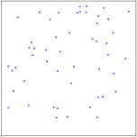
(a) initial configuration

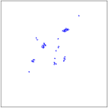
(b) after $60$ $\mathrm{s}$

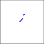
(c) after $180$ $\mathrm{s}$

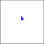
(d) after $300$ $\mathrm{s}$

Figure 2: Snapshots of the aggregation behavior of $50$ agents in simulation.

When $I=0$, an agent moves backwards along a clockwise circular trajectory ($v_{\ell 0}=-0.7$ and $v_{r0}=-1.0$). When $I=1$, an agent rotates clockwise on the spot with maximum angular speed ($v_{\ell 1}=1.0$ and $v_{r1}=-1.0$). Note that, rather counterintuitively, an agent never moves forward, regardless of $I$. With this controller, an agent provably aggregates with another agent or with a quasi-static cluster of agents (Gauci et al., 2014c). Fig. 2 shows snapshots from a simulation trial with $50$ agents.

Object Clustering: In this behavior, the sensor is ternary, that is, $n=3$. It gives a reading of $I=2$ if there is an agent in the line of sight, $I=1$ if there is an object in the line of sight, and $I=0$ otherwise. The objective of the agents is to arrange the objects into a single compact cluster as fast as possible. Details of this behavior, including a validation using 5 physical e-puck robots and 20 cylindrical objects, are presented in (Gauci et al., 2014b).

The controller’s parameters, found using an evolutionary algorithm (Gauci et al., 2014b), are:

$$\mathbf{p}=\left(0.5,1.0,1.0,0.5,0.1,0.5\right).$$ (7)

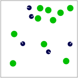
(a) initial configuration

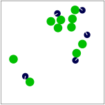
(b) after $20$ $\mathrm{s}$

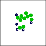
(c) after $40$ $\mathrm{s}$

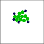
(d) after $60$ $\mathrm{s}$

Figure 3: Snapshots of the object clustering behavior in simulation. There are $5$ agents (dark blue) and 10 objects (green).

When $I=0$ and $I=2$, the agent moves forward along a counterclockwise circular trajectory, but with different linear and angular speeds. When $I=1$, it moves forward along a clockwise circular trajectory. Fig. 3 shows snapshots from a simulation trial with $5$ agents and $10$ objects.

3.2.2 Models and replicas

We assume the availability of replicas, which must have the potential to produce data samples that—to an external observer (classifier)—are indistinguishable from those of the agent. In our case, the replicas have the same morphology as the agent, including identical line-of-sight sensors and differential drive mechanisms.

The replicas execute behavioral rules defined by the model. We adopt two model representations: gray box and black box. In both cases, note that the classifiers, which determine the quality of the models, have no knowledge about the agent/model representation or the agent/model inputs.

• In a gray box representation, the agent’s control system structure is assumed to be known. In other words, the model and the agent share the same control system structure, as defined in Eq. (5). This representation reduces the complexity of the identification process, in the sense that only the parameters of Eq. (5) need to be inferred. Additionally, this allows for an objective evaluation of how well the identification process performs, because one can compare the inferred parameters directly with the ground truth.

• In a black box representation, the agent’s control system structure is assumed to be unknown, and the model has to be represented in a general way. In particular, we use a control system structure with memory, in the form of a neural network with recurrent connections (see Section 4.6.2).

The replicas can be mixed into a group of agents or separated from them. By default, we consider the situation that one or multiple replicas are mixed into a group of agents. The case of studying groups of agents and groups of replicas in isolation is investigated in Section 4.6.3.

3.2.3 Classifiers

The classifiers need to discriminate between data samples originating from the agents and ones originating from the replicas. We use the term individual to refer to either the agent or a replica executing a model.

A data sample comes from the motion trajectory of an individual observed for the duration of a trial. We assume that it is possible to track both the individual’s position and orientation. The sample comprises the linear speed ($s$) and angular speed ($\omega$). Full details (e.g., trial duration) are provided in Sections 4.2 and 5.3 for the cases of simulation and physical experiments respectively.

The classifier is represented as an Elman neural network (Elman, 1990). The network has $i=2$ inputs ($s$ and $\omega$), $h=5$ hidden neurons and one output neuron. Each neuron of the hidden and output layers has a bias. The network thus has a total of $(i+1)h+h^{2}+(h+1)=46$ parameters, which all assume values in $\mathbb{R}$. The activation function used in the hidden and the output neurons is the logistic sigmoid function, which has the range $\left(0,1\right)$ and is defined as:

$$\textrm{sig}\,(x)=\frac{1}{1+e^{-x}},\quad\forall x\in\mathbb{R}.$$ (8)

The data sample consists of a time series, which is fed sequentially into the classifier neural network. The final value of the output neuron is used to make the judgment: model, if its value is less than $0.5$, and agent otherwise. The network’s memory (hidden neurons) is reset after each judgment.

3.2.4 Optimization algorithm

The optimization of models and classifiers is realized using an evolutionary algorithm. We use a ($\mu+\lambda$) evolution strategy with self-adaptive mutation strengths (Eiben and Smith, 2003) to optimize either population. As a consequence, the optimization consists of two processes, one for the model population, and another for the classifier population. The two processes synchronize whenever the solution qualities described in Section 3.1 are computed. The implementation of the evolutionary algorithm is detailed in (Li et al., 2013).

For the remainder of this paper, we adopt terminology used in evolutionary computing, and refer to the quality of solutions as their fitness and to iteration cycles as generations. Note that in coevolutionary algorithms, each population’s fitness depends on the performance of the other populations, and is hence referred to as the subjective fitness. By contrast, the fitness measure as used in conventional evolutionary algorithms is referred to as the objective fitness.

3.2.5 Termination criterion

The algorithm stops after running for a fixed number of iterations.

4 Simulation experiments

In this section, we present the simulation experiments for the two case studies. Sections 4.1 and 4.2 describe the simulation platform and setups. Sections 4.3 and 4.4, respectively, analyze the inferred models and classifiers. Section 4.5 compares Turing Learning with a metric-based identification method and mathematically analyzes this latter method. Section 4.6 presents further results of testing the generality of Turing Learning through exploring different scenarios, which include: (i) simultaneously inferring the control of the agent and an aspect of its morphology; (ii) using artificial neural networks as a model representation, thereby removing the assumption of a known agent control system structure; (iii) separating the replicas and the agents, thereby allowing for a potentially simpler experimental setup; and (iv) inferring arbitrary reactive behaviors.

4.1 Simulation platform

We use the open-source Enki library (Magnenat et al., 2011), which models the kinematics and dynamics of rigid objects, and handles collisions. Enki has a built-in 2D model of the e-puck. The robot is represented as a disk of diameter $7.0\,\mathrm{cm}$ and mass $150\,\mathrm{g}$. The inter-wheel distance is $5.1\,\mathrm{cm}$. The speed of each wheel can be set independently. Enki induces noise on each wheel speed by multiplying the set value by a number in the range $(0.95,1.05)$ chosen randomly with uniform distribution. The maximum speed of the e-puck is $12.8\,\mathrm{\textrm{cm/s}}$, forwards or backwards. The line-of-sight sensor is simulated by casting a ray from the e-puck’s front and checking the first item with which it intersects (if any). The range of this sensor is unlimited in simulation.

In the object clustering case study, we model objects as disks of diameter $10\,\mathrm{cm}$ with mass $35\,\mathrm{g}$ and a coefficient of static friction with the ground of $0.58$, which makes it movable by a single e-puck.

The robot’s control cycle is updated every $0.1\,\mathrm{s}$, and the physics is updated every $0.01\,\mathrm{s}$.

4.2 Simulation setups

In all simulations, we use an unbounded environment. For the aggregation case study, we use groups of $11$ individuals—$10$ agents and $1$ replica that executes a model. The initial positions of individuals are generated randomly in a square region of sides $331.66\,\mathrm{cm}$, following a uniform distribution (average area per individual = $10000\,\mathrm{cm^{2}}$). For the object clustering case study, we use groups of $5$ individuals—$4$ agents and $1$ replica that executes a model—and $10$ cylindrical objects. The initial positions of individuals and objects are generated randomly in a square region of sides $100\,\mathrm{cm}$, following a uniform distribution (average area per object = $1000\,\mathrm{cm^{2}}$). In both case studies, individual starting orientations are chosen randomly in $[-\pi,\pi)$ with uniform distribution.

We performed 30 runs of Turing Learning for each case study. Each run lasted 1000 generations. The model and classifier populations each consisted of $100$ solutions ($\mu=50$, $\lambda=50$). In each trial, classifiers observed individuals for $10\,\mathrm{s}$ at $0.1\,\mathrm{s}$ intervals ($100$ data points). In both setups, the total number of samples for the agents in each generation was equal to $n_{t}\times n_{a}$, where $n_{t}$ is the number of trials performed (one per model) and $n_{a}$ is the number of agents in each trial.

4.3 Analysis of inferred models

In order to objectively measure the quality of the models obtained through Turing Learning, we define two metrics. Given a candidate model (candidate controller) $\mathbf{x}$ and the agent (original controller) $\mathbf{p}$, where $\mathbf{x}\in\mathbb{R}^{2n}$ and $\mathbf{p}\in[-1,1]^{2n}$, we define the absolute error (AE) in a particular parameter $i\in\{1,2,\dots,2n\}$ as:

$$\mathrm{AE}_{i}=|x_{i}-p_{i}|.$$ (9)

We define the mean absolute error (MAE) over all parameters as:

$$\mathrm{MAE}=\frac{1}{2n}\sum_{i=1}^{2n}\mathrm{AE}_{i}.$$ (10)

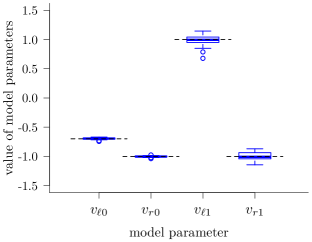
(a) (a) Aggregation

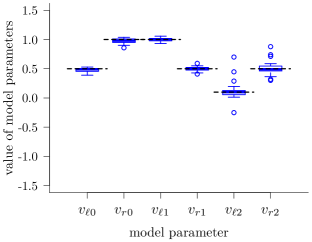
(b) (b) Object Clustering

Figure 4: Model parameters Turing Learning inferred from swarms of simulated agents performing (a) aggregation and (b) object clustering. Each box corresponds to the models with the highest subjective fitness in the $1000$th generation of 30 runs. The dashed black lines correspond to the values of the parameters that the system is expected to learn (i.e., those of the agent).

Fig. 4 shows a box plot of the parameters of the inferred models with the highest subjective fitness value in the final generation. It can be seen that Turing Learning identifies the parameters for both behaviors with good accuracy (dashed black lines represent the ground truth, that is, the parameters of the observed swarming agents). In the case of aggregation, the means (standard deviations) of the AEs in the parameters are (from left to right in Fig. LABEL:sub@fig:model_parameters_box_aggregation): $0.01$ ($0.01$), $0.01$ ($0.01$), $0.07$ ($0.07$), and $0.06$ ($0.04$). In the case of object clustering, these values are as follows: $0.03$ ($0.03$), $0.04$ ($0.03$), $0.02$ ($0.02$), $0.03$ ($0.03$), $0.08$ ($0.13$), and $0.08$ ($0.09$).

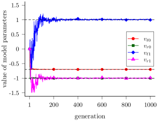
(a) (a) Aggregation

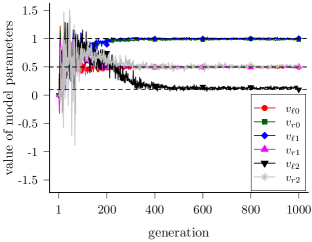
(b) (b) Object Clustering

Figure 5: Evolutionary dynamics of model parameters for the (a) aggregation and (b) object clustering case studies. Curves represent median parameter values of the models with the highest subjective fitness across 30 runs of Turing Learning. Dashed black lines indicate the ground truth.

We also investigate the evolutionary dynamics. Fig. 5 shows how the model parameters converge over generations. In the aggregation case study (see Fig. LABEL:sub@fig:model_parameters_convergence_aggregation), the parameters corresponding to $I=0$ are learned first. After around $50$ generations, both $v_{\ell 0}$ and $v_{r0}$ closely approximate their true values ($-0.7$ and $-1.0$). For $I=1$, it takes about $200$ generations for both $v_{\ell 1}$ and $v_{r1}$ to converge. A likely reason for this effect is that an agent spends a larger proportion of its time seeing nothing ($I=0$) than seeing other agents ($I=1$)—simulations revealed these percentages to be $91.2\%$ and $8.8\%$ respectively (mean values over $100$ trials).

In the object clustering case study (see Fig. LABEL:sub@fig:model_parameters_convergence_clustering), the parameters corresponding to $I=0$ and $I=1$ are learned faster than the parameters corresponding to $I=2$. After about $200$ generations, $v_{\ell 0}$, $v_{r0}$, $v_{\ell 1}$ and $v_{r1}$ start to converge; however it takes about $400$ generations for $v_{\ell 2}$ and $v_{r2}$ to approximate their true values. Note that an agent spends the highest proportion of its time seeing nothing ($I=0$), followed by seeing objects ($I=1$) and seeing other agents ($I=2$)—simulations revealed these proportions to be $53.2\%$, $34.2\%$ and $12.6\%$ respectively (mean values over $100$ trials).

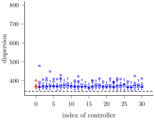
(a) (a) Aggregation

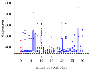
(b) (b) Object Clustering

Figure 6: (a) Dispersion of $50$ simulated agents (red box) or replicas (blue boxes), executing one of the $30$ inferred models in the aggregation case study. (b) Dispersion of $50$ objects when using a swarm of $25$ simulated agents (red box) or replicas (blue boxes), executing one of the $30$ inferred models in the object clustering case study. In both (a) and (b), boxes show the distributions obtained after $400\,\mathrm{s}$ over $30$ trials. The models are from the $1000$th generation. The dashed black lines indicate the minimum dispersion that $50$ individuals/objects can possibly achieve (Graham and Sloane, 1990). See Section 4.3 for details.

Although the inferred models approximate the agents well in terms of parameters, it is not uncommon in swarm systems that small changes in individual behavior lead to vastly different emergent behaviors, especially when using large numbers of agents (Levi and Kernbach, 2010). For this reason, we evaluate the quality of the emergent behaviors that the models give rise to. In the case of aggregation, we measure the dispersion of the swarm after some elapsed time as defined in (Gauci et al., 2014c). For each of the $30$ models with the highest subjective fitness in the final generation, we performed $30$ trials with $50$ replicas executing the model. For comparison, we also performed $30$ trials using the agent (see Eq. (6)). The set of initial configurations was the same for the replicas and the agents. Fig. LABEL:sub@fig:model_validation_aggregation_simulation shows the dispersion of agents and replicas after $400\,\mathrm{s}$. All models led to aggregation. We performed a statistical test on the final dispersion of the individuals between the agents and replicas for each model. There is no statistically significant difference in $30$ out of $30$ cases (tests with Bonferroni correction).

In the case of object clustering, we use the dispersion of the objects after $400\,\mathrm{s}$ as a measure of the emergent behavior. We performed $30$ trials with $25$ individuals and $50$ objects for the agent and each model. The results are shown in Fig. LABEL:sub@fig:model_validation_clustering_simulation. In the final dispersion of objects by the agent or any of the models (replicas), there is no statistically significant difference in $26$ out of $30$ cases (tests with Bonferroni correction).

4.4 Analysis of generated classifiers

The primary outcome of the Turing Learning method (and of any system identification method) is the model, which has been discussed in the previous section. However, the generated classifiers can also be considered as a useful by-product. For instance they could be used to detect abnormal agents in a swarm. We now analyze the performance of the classifiers. For the remainder of this paper, we consider only the aggregation case study.

To assess the performance of the classifiers, we measure the percentage of correct judgments over agents and a wide range of models. The models are uniformly distributed over the four-dimensional parameter space of the agents (see Eqs. (5) and (6)); each element takes a value in $[-1,1]$. To keep the analysis of classifiers within a reasonable computation time, we discretize this space using $11$ settings per parameter; thus, each parameter is chosen from the set $\{-1.0,-0.8,...,0.8,1.0\}$. This discretized space is a grid consisting of $|\mathcal{X}|=11^{4}=14641$ points (i.e., models). The model is executed by a replica mixed into a group of $10$ agents (as in the Turing Learning runs). The motion data are fed to each classifier, which makes $10$ judgments per individual. If the classifier consistently judges the individual as a model (i.e., not an agent) in $10$ out of $10$ trials, it outputs a “model” decision. Otherwise, it outputs “agent”. This conservative approach is used to minimize the risk of false-positive detection of abnormal behavior. The classifier’s performance (i.e., decision accuracy) is computed by combining the percentage of correct judgments about models ($50\%$ weight) with the percentage of correct judgments about agents ($50\%$ weight), analogous to the solution quality definition in Eq. (2).

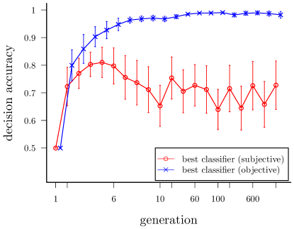
Figure 7: Average decision accuracy of the best classifiers over $1000$ generations (nonlinear scale) in $30$ runs of Turing Learning. The error bars show standard deviations. See text for details.

We performed $10$ trials using a set of initial configurations common to all classifiers. Fig. 7 shows the average decision accuracy of the classifier with the highest subjective fitness during the evolution (best classifier (subjective)) in $30$ runs of Turing Learning. The accuracy of the classifier increases in the first $5$ generations, then drops, and fluctuates within range $62\%$–$80\%$. For a comparison, we also plot the highest decision accuracy that a single classifier achieved during the post-evaluation for each generation. This classifier is referred to best classifier (objective). Interestingly, the accuracy of the best classifier (objective) increases almost monotonically, reaching a level above $95\%$. To select the best classifier (objective), all the classifiers were post-evaluated using the aforementioned $14641$ models.

At first sight, it seems counterintuitive that the best classifier (subjective) has a low decision accuracy. This phenomenon, however, can be explained when considering the model population. We have shown in the previous section (see Fig. LABEL:sub@fig:model_parameters_convergence_aggregation) that the models converge rapidly at the beginning of the coevolutions. As a result, when classifiers are evaluated in later generations, the trials are likely to include models very similar to each other. Classifiers that become overspecialized to this small set of models (the ones dominating the later generations) have a higher chance of being selected during the evolutionary process. These classifiers may however have a low performance when evaluated across the entire model space.

Note that our analysis does not exclude the potential existence of models for which the performance of the classifiers degenerates substantially. As reported by (Nguyen et al., 2015), well-trained classifiers, which in their case are represented by deep neural networks, can be easily fooled. For instance, the classifiers may label a random-looking image as a guitar with high confidence. However, in this degenerate case, the image was obtained through evolutionary learning, while the classifiers remained static. By contrast, in Turing Learning, the classifiers are coevolving with the models, and hence have the opportunity to adapt to such a situation.

4.5 A metric-based system identification method: mathematical analysis and comparison with Turing Learning

In order to compare Turing Learning against a metric-based method, we employ the commonly used least-square approach. The objective is to minimize the differences between the observed outputs of the agents and of the models, respectively. Two outputs are considered—an individual’s linear and angular speed. Both outputs are considered over the whole duration of a trial. Formally,

$${e_{m}=\sum\limits_{i=1}^{n_{a}}\sum\limits_{t=1}^{T}\left\{(s_{m}^{(t)}-s_{i}^{(t)})^{2}+(\omega_{m}^{(t)}-\omega_{i}^{(t)})^{2}\right\},}$$ (11)

where $s_{m}^{(t)}$ and $s_{i}^{(t)}$ are the linear speed of the model and of agent $i$, respectively, at time step $t$; $\omega_{m}^{(t)}$ and $\omega_{i}^{(t)}$ are the angular speed of the model and of agent $i$, respectively, at time step $t$; $n_{a}$ is the number of agents in the group; $T$ is the total number of time steps in a trial.

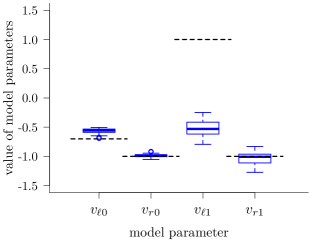
(a) (a) Aggregation

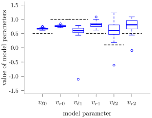
(b) (b) Object Clustering

Figure 8: Model parameters a metric-based evolutionary method inferred from swarms of simulated agents performing (a) aggregation and (b) object clustering. Each box corresponds to the models with the highest fitness in the $1000$th generation of 30 runs. The dashed black lines correspond to the values of the parameters that the system is expected to learn (i.e., those of the agent).

4.5.1 Mathematical analysis

We begin our analysis by first analyzing an abstract version of the problem.

Theorem 1.

Consider two binary random variables $X$ and $Y$. Variable $X$ takes value $x_{1}$ with probability $p$, and value $x_{2}$, otherwise. Variable $Y$ takes value $y_{1}$ with the same probability $p$, and value $y_{2}$, otherwise. Variables $X$ and $Y$ are assumed to be independent of each other. Assuming $y_{1}$ and $y_{2}$ are given, then the metric $D=\mathbb{E}\{(X-Y)^{2}\}$ has a global minimum at $X^{*}$ with $x_{1}^{*}=x_{2}^{*}=\mathbb{E}\{Y\}$. If $p\in(0,1)$, the solution is unique.

Proof.

The probability of (i) both $x_{1}$ and $y_{1}$ being observed is $p^{2}$; (ii) both $x_{1}$ and $y_{2}$ being observed is $p(1-p)$; (iii) both $x_{2}$ and $y_{1}$ being observed is $(1-p)p$; (iv) both $x_{2}$ and $y_{2}$ being observed is $(1-p)^{2}$. The expected error value, $D$, is then given as

$$D=p^{2}\left(x_{1}-y_{1}\right)^{2}+p(1-p)\left(x_{1}-y_{2}\right)^{2}+(1-p)p\left(x_{2}-y_{1}\right)^{2}+(1-p)^{2}\left(x_{2}-y_{2}\right)^{2}.$$ (12)

To find the minimum expected error value, we set the partial derivatives w.r.t. $x_{1}$ and $x_{2}$ to $0$. For $x_{1}$, we have:

$$\frac{\partial D}{\partial x_{1}}=2p^{2}\left(x_{1}-y_{1}\right)+2p(1-p)\left(x_{1}-y_{2}\right)=0,$$ (13)

from which we obtain $x^{*}_{1}=py_{1}+(1-p)y_{2}=\mathbb{E}\{Y\}$. Similarly, setting $\frac{\partial D}{\partial x_{2}}=0$ we obtain $x^{*}_{2}=py_{1}+(1-p)y_{2}=\mathbb{E}\{Y\}$. Note that at these values of $x_{1}$ and $x_{2}$, the second-order partial derivatives are both positive (assuming $p\in(0,1)$). Therefore, the (global) minimum of $D$ is at this stationary point. ∎

Corollary 1.

If $p\in(0,1)$ and $y_{1}\neq y_{2}$, then $X^{*}\neq Y$.

Proof.

As $p\in(0,1)$, the only global minimum exists at $X^{*}$. As $x^{*}_{1}=x^{*}_{2}$ and $y_{1}\neq y_{2}$, it follows that $X^{*}\neq Y$. ∎

Corollary 2.

Consider two discrete random variables $X$ and $Y$ with values $x_{1}$, $x_{2},\ldots,x_{n}$, and $y_{1}$, $y_{2},\ldots,y_{n}$ respectively, $n>1$. Variable $X$ takes value $x_{i}$ with probability $p_{i}$ and variable $Y$ takes value $y_{i}$ with the same probability $p_{i}$, $i=1,2,\dots,n$, where $\sum\limits_{i=1}^{n}p_{i}=1$ and $\exists i,j:y_{i}\neq y_{j}$. Variables $X$ and $Y$ are assumed to be independent of each other. Metric $D$ has a global minimum at $X^{*}\neq Y$ with $x_{1}^{*}=x_{2}^{*}=\ldots=x_{n}^{*}=\mathbb{E}\{Y\}$. If all $p_{i}\in(0,1)$, then $X^{*}$ is unique.

Proof.

This proof, which is omitted here, can be obtained by examining the first and second derivatives of a generalized version of Eq. (12). Rather than four ($2^{2}$) cases, there are $n^{2}$ cases to be considered. ∎

Corollary 3.

Consider a sequence of pairs of binary random variables ($X_{t}$, $Y_{t}$), $t=1,\ldots,T$. Variable $X_{t}$ takes value $x_{1}$ with probability $p_{t}$, and value $x_{2}$, otherwise. Variable $Y_{t}$ takes value $y_{1}$ with the same probability $p_{t}$, and value $y_{2}\neq y_{1}$, otherwise. For all $t$, variables $X_{t}$ and $Y_{t}$ are assumed to be independent of each other. If all $p_{t}\in(0,1)$, then the metric $D=\mathbb{E}\left\{\sum_{t=1}^{T}(X_{t}-Y_{t})^{2}\right\}$ has one global minimum at $X^{*}\neq Y$.

Proof.

The case $T=1$ has already been considered (Theorem 1 and Corollary 1). For the case $T=2$, we extend Eq. (13) to take into account $p_{1}$ and $p_{2}$, and obtain

$$x_{1}(p_{1}^{2}+p_{1}-p_{1}^{2}+p_{2}^{2}+p_{2}-p_{2}^{2})=y_{1}(p_{1}^{2}+p_{2}^{2})+y_{2}(p_{1}-p_{1}^{2}+p_{2}-p_{2}^{2}).$$ (14)

This can be rewritten as:

$$x_{1}=\frac{p_{1}^{2}+p_{2}^{2}}{p_{1}+p_{2}}y_{1}+\frac{p_{1}(1-p_{1})+p_{2}(1-p_{2})}{p_{1}+p_{2}}y_{2}.$$ (15)

As $y_{2}\neq y_{1}$, $x_{1}$ can only be equal to $y_{1}$ if $p_{1}^{2}+p_{2}^{2}=p_{1}+p_{2}$, which is equivalent to $p_{1}(1-p_{1})+p_{2}(1-p_{2})=0$. This is however not possible for any $p_{1},p_{2}\in(0,1)$. Therefore, $X^{*}\neq Y$.

For the general case, $T\geq 1$, the following equation can be obtained (proof omitted).

$$x_{1}=\frac{\sum_{t=1}^{T}p_{t}^{2}}{\sum_{t=1}^{T}p_{t}}y_{1}+\frac{\sum_{t=1}^{T}p_{t}(1-p_{t})}{\sum_{t=1}^{T}p_{t}}y_{2}.$$ (16)

The same argument applies—$x^{*}_{1}$ cannot be equal to $y_{1}$. Therefore, $X^{*}\neq Y$. ∎

Implications for our scenario: The metric-based approach considered in this paper is unable to infer the correct behavior of the agent. In particular, the model that is globally optimal w.r.t. the expected value for the error function defined by Eq. (11) is different from the agent. This observation follows from Corollary 1 for the aggregation case study (two sensor states), and from Corollary 2 for the object clustering case study (three sensor states). It exploits the fact that the error function is of the same structure as the metric in Corollary 3—a sum of square error terms. The summation over time is not of concern—as was shown in Corollary 3, the distributions of sensor reading values (inputs) of the agent and of the model do not need to be stationary. However, we need to assume that for any control cycle, the actual inputs of agents and models are not correlated with each other. Note that the sum in Eq. (11) comprises two square error terms: one for the linear speed of the agent, and the other for the angular speed. As our simulated agents employ a differential drive with unconstrained motor speeds, the linear and angular speeds are decoupled. In other words, the linear and angular speeds can be chosen independently of each other, and optimized separately. This means that Eq. (11) can be thought of as two separate error functions: one pertaining to the linear speeds, and the other to the angular speeds.

4.5.2 Comparison with Turing Learning

To verify whether the theoretical result (and its assumptions) holds in practice, we used an evolutionary algorithm with a single population of models. The algorithm was identical to the model optimization sub-algorithm in Turing Learning except for the fitness calculation, where the metric of Eq. 11 was employed. We performed 30 evolutionary runs for each case study. Each evolutionary run lasted $1000$ generations. The simulation setup and number of fitness evaluations for the models were kept the same as in Turing Learning.

Fig. LABEL:sub@fig:model_parameters_box_aggregation_evolution shows the parameter distribution of the evolved models with highest fitness in the last generation over $30$ runs. The distributions of the evolved parameters corresponding to $I=0$ and $I=1$ are similar. This phenomenon can be explained as follows. In the identification problem that we consider, the method has no knowledge of the input, that is, whether the agent perceives another agent ($I=1$) or not ($I=0$). This is consistent with Turing Learning as the classifiers that are used to optimize the models also do not have any knowledge of the inputs. The metric-based algorithm seems to construct controllers that do not respond differently to either input, but work as good as it gets on average, that is, for the particular distribution of inputs, $0$ and $1$. For the left wheel speed both parameters are approximately $-0.54$. This is almost identical to the weighted mean ($-0.7*0.912+1.0*0.088=-0.5504$), which takes into account that parameter $v_{\ell 0}=-0.7$ is observed around 91.2% of the time, whereas parameter $v_{\ell 1}=1$ is observed around 8.8% of the time (see also Section 4.3). The parameters related to $I=1$ evolved well as the agent’s parameters are identical regardless of the input ($v_{r0}=v_{r1}=-1.0$). For both $I=0$ and $I=1$, the evolved parameters show good agreement with Theorem 1. As the model and the agents are only observed for $10\,\mathrm{s}$ in the simulation trials, the probabilities of seeing a $0$ or a $1$ are nearly constant throughout the trial. Hence, this scenario approximates very well the conditions of Theorem 1, and the effects of non-stationary probabilities on the optimal point (Corollary 3) are minimal. Similar results were found when inferring the object clustering behavior (see Fig. LABEL:sub@fig:model_parameters_box_clustering_evolution).

By comparing Figs. 4 and 8, one can see that Turing Learning outperforms the metric-based evolutionary algorithm in terms of model accuracy in both case studies. As argued before, due to the unpredictable interactions in swarms the traditional metric-based method is not suited for inferring the behaviors.

4.6 Generality of Turing Learning

In the following, we present four orthogonal studies testing the generality of Turing Learning. The experimental setup in each section is identical to that described previously (see Section 4.2), except for the modifications discussed within each section.

4.6.1 Simultaneously inferring control and morphology

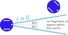
(a) (a)

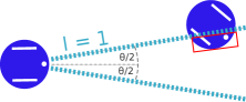
(b) (b)

Figure 9: A diagram showing the angle of view of the agent’s sensor investigated in Section 4.6.1.

In the previous sections, we assumed that we fully knew the agents’ morphology, and only their behavior (controller) was to be identified. We now present a variation where one aspect of the morphology is also unknown. The replica, in addition to the four controller parameters, takes a parameter $\theta\in\left[0,2\pi\right]\mathrm{rad}$, which determines the horizontal field of view of its sensor, as shown in Fig. 9 (the sensor is still binary). Note that the agents’ line-of-sight sensors of the previous sections can be considered as sensors with a field of view of $0\,\mathrm{rad}$.

The models now have five parameters. As before, we let Turing Learning run in an unbounded search space (i.e., now, $\mathbb{R}^{5}$). However, as $\theta$ is necessarily bounded, before a model is executed on a replica, the parameter corresponding to $\theta$ is mapped to the range $(0,2\pi)$ using an appropriately scaled logistic sigmoid function. The controller parameters are directly passed to the replica. In this setup, the classifiers observe the individuals for $100\,\mathrm{s}$ in each trial (preliminary results indicated that this setup required a longer observation time).

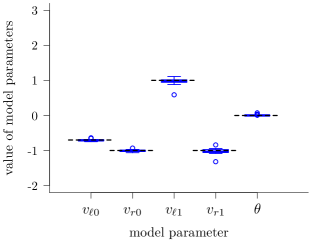
(a) (a)

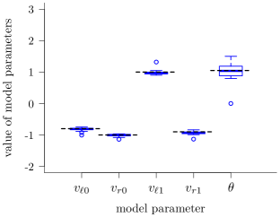
(b) (b)

Figure 10: Turing Learning simultaneously inferring control and morphological parameters (field of view). The agents’ field of view is (a) $0\,\mathrm{rad}$ and (b) $\pi/3\,\mathrm{rad}$. Boxes show distributions for the models with the highest subjective fitness in the $1000$th generation over $30$ runs. Dashed black lines indicate the ground truth.

Fig. LABEL:sub@fig:model_parameters_box_aggregation_0degree shows the parameters of the subjectively best models in the last ($1000$th) generations of $30$ runs. The means (standard deviations) of the AEs in each model parameter are as follows: $0.02$ ($0.01$), $0.02$ ($0.02$), $0.05$ ($0.07$), $0.06$ ($0.06$), and $0.01$ ($0.01$). All parameters including $\theta$ are still learned with high accuracy.

The case where the true value of $\theta$ is $0\,\mathrm{rad}$ is an edge case, because given an arbitrarily small $\epsilon>0$, the logistic sigmoid function maps an unbounded domain of values onto $(0,\epsilon)$. This makes it simpler for Turing Learning to infer this parameter. For this reason, we also consider another scenario where the agents’ angle of view is $\pi/3\,\mathrm{rad}$ rather than $0\,\mathrm{rad}$. The controller parameters for achieving aggregation in this case are different from those in Eq. (6). They were found by rerunning a grid search with the modified sensor. Fig. LABEL:sub@fig:model_parameters_box_aggregation_60degree shows the results from $30$ runs with this setup. The means (standard deviations) of the AEs in each parameter are as follows: $0.04$ ($0.04$), $0.03$ ($0.03$), $0.05$ ($0.06$), $0.05$ ($0.05$), and $0.20$ ($0.19$). The controller parameters are still learned with good accuracy. The accuracy in the angle of view is noticeably lower, but still reasonable.

4.6.2 Inferring behavior without assuming a known control system structure

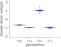
(a) (a) One hidden neuron

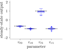
(b) (b) Three hidden neurons

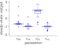
(c) (c) Five hidden neurons

Figure 11: Turing Learning can infer an agent’s behavior without assuming its control system structure to be known. These plots show the steady-state outputs (in the $20$th time step) of the inferred neural networks with the highest subjective fitness in the $1000$th generation of 30 simulation runs. Two outliers in (c) are not shown.

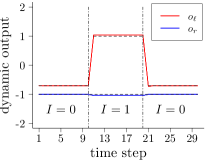
(a) (a) One hidden neuron

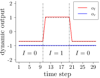
(b) (b) Three hidden neurons

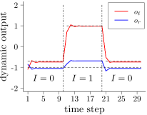
(c) (c) Five hidden neurons

Figure 12: Dynamic outputs of the inferred neural network with median performance. The network’s input in each case was $I=0$ (time steps 1–10), $I=1$ (time steps 11-20) and $I=0$ (time steps 21–30). See text for details.

In the previous sections, we assumed the agent’s control system structure to be known and only inferred its parameters. To further investigate the generality of Turing Learning, we now represent the model in a more general form, namely a (recurrent) Elman neural network (Elman, 1990). The network inputs and outputs are identical to those used for our reactive models. In other words, the Elman network has one input ($I$) and two outputs representing the left and right wheel speed of the robot. A bias is connected to the input and hidden layers of the network, respectively. We consider three network structures with one, three, and five hidden neurons, which correspond, respectively, to $7$, $23$ and $47$ weights to be optimized. Except for a different number of parameters to be optimized, the experimental setup is equivalent in all aspects to that of Section 4.2.

We first analyze the steady-state behavior of the inferred network models. To obtain their steady-state outputs, we fed them with a constant input ($I=0$ or $I=1$ depending on the parameters) for $20$ time steps. Fig. 11 shows the outputs in the final time step of the inferred models with the highest subjective fitness in the last generation in $30$ runs for the three cases. In all cases, the parameters of the swarming agent can be inferred correctly with reasonable accuracy. More hidden neurons lead to worse results, probably due to the larger search space.

We now analyze the dynamic behavior of the inferred network models. Fig. 12 shows the dynamic output of $1$ of the $30$ neural networks. The chosen neural network is the one exhibiting the median performance according to metric $\sum\limits_{i=1}^{4}\sum\limits_{t=1}^{20}(o_{it}-p_{i})^{2}$, where $p_{i}$ denotes the $i$th parameter in Eq. (6), and $o_{it}$ denotes the output of the neural network in the $t$th time step corresponding to the $i$th parameter in Eq. (6). The inferred networks react to the inputs rapidly and maintain a steady-state output (with little disturbance). The results show that Turing Learning can infer the behavior without assuming the agent’s control system structure to be known.

4.6.3 Separating the replicas and the agents

In our two case studies, the replica was mixed into a group of agents. In the context of animal behavior studies, a robot replica may be introduced into a group of animals and recognized as a conspecific (Halloy et al., 2007; Faria et al., 2010). However, if behaving abnormally, the replica may disrupt the behavior of the swarm (Bjerknes and Winfield, 2013). For the same reason, the insertion of a replica that exhibits different behavior or is not recognized as conspecific may disrupt the behavior of the swarm and hence the models obtained may be biased. In this case, an alternative method would be to isolate the influence of the replica(s). We performed an additional simulation study where agents and replicas were never mixed. Instead, each trial focused on either a group of agents, or of replicas. All replicas in a trial executed the same model. The group size was identical in both cases. The tracking data of the agents and the replicas from each sample were then fed into the classifiers for making judgments.

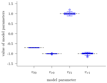
Figure 13: Model parameters inferred by a variant of Turing Learning that observes swarms of aggregating agents and swarms of replicas in isolation, thereby avoiding potential bias. Each box corresponds to the models with the highest subjective fitness in the $1000$th generation of 30 simulation runs.

The distribution of the inferred model parameters is shown in Fig. 13. The results show that Turing Learning can still identify the model parameters well. There is no significant difference between either approach in the case studies considered in this paper. The method of separating replicas and agents is recommended if potential biases are suspected.

4.6.4 Inferring other reactive behaviors

The aggregation controller that agents used in our case study was originally synthesized by searching over the parameter space defined in Eq. (5) with $n=2$, using a metric to assess the swarm’s global performance (Gauci et al., 2014c). Each of these points produces a global behavior. Some of these behaviors are particularly interesting, such as the circle formation behavior reported in (Gauci et al., 2014a).

We now investigate whether Turing Learning can infer arbitrary controllers in this space, irrespective of the global behaviors they lead to. We generated $1000$ controllers randomly in the parameter space defined in Eq. (5), with uniform distribution. For each controller, we performed one run, and selected the subjectively best model in the last ($1000$th) generation.

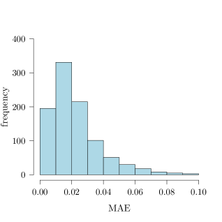
(a) (a)

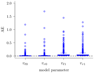
(b) (b)

Figure 14: Turing Learning inferring the models for 1000 randomly generated agent behaviors. For each behavior, one run of Turing Learning was performed and the model with the highest subjective fitness after $1000$ generations was considered. (a) Histogram of the models’ MAE (defined in Eq. (10); $43$ points that have an MAE larger than $0.1$ are not shown); and (b) AEs (defined in Eq. (9)) for each model parameter.

Fig. LABEL:sub@fig:MAE_histgram_random_controllers shows a histogram of the MAE of the inferred models. The distribution has a single mode close to zero, and decays rapidly for increasing values. Over $89\%$ of the $1000$ cases have an error below $0.05$. This suggests that the accuracy of Turing Learning is not highly sensitive to the particular behavior under investigation (i.e., most behaviors are learned equally well). Fig. LABEL:sub@fig:AE_box_random_controllers shows the AEs of each model parameter. The means (standard deviations) of the AEs in each parameter are as follows: $0.01$ ($0.05$), $0.02$ ($0.07$), $0.07$ ($0.6$), and $0.05$ ($0.2$). We performed a statistical test on the AEs between the model parameters corresponding to $I=0$ ($v_{\ell 0}$ and $v_{r0}$) and $I=1$ ($v_{\ell 1}$ and $v_{r1}$). The AEs of the inferred $v_{\ell 0}$ and $v_{r0}$ are significantly lower than those of $v_{\ell 1}$ and $v_{r1}$. This is likely due to the reason reported in Section 4.3; that is, an agent is likely to spend more time seeing nothing ($I=0$) than seeing other agents ($I=1$) in each trial.

5 Physical experiments

In this section, we present a real-world validation of Turing Learning. We explain how it can be used to infer the behavior of a swarm of real agents. The agents and replicas are represented by physical robots. We use the same type of robot (e-puck) as in simulation. The agents execute the aggregation behavior described in Section 3.2.1. The replicas execute the candidate models. We use two replicas to speed up the identification process, as will be explained in Section 5.3.

5.1 Physical platform

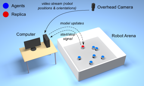
Figure 15: Illustration of the general setup for inferring the behavior of physical agents—e-puck robots (not to scale). The computer runs the Turing Learning algorithm, which produces models and classifiers. The models are uploaded and executed on the replica. The classifiers run on the computer. They are provided with the agents’ and replica’s motion data, extracted from the video stream of the overhead camera.

The physical setup, shown in Fig. 15, consists of an arena with robots (representing agents or replicas), a personal computer (PC), and an overhead camera. The PC runs the Turing Learning algorithm. It communicates with the replicas, providing them models to be executed, but does not exert any control over the agents. The overhead camera supplies the PC with a video stream of the swarm. The PC performs video processing to obtain motion data about individual robots. We now describe the physical platform in more detail.

5.1.1 Robot arena

The robot arena is rectangular with sides $200\,\mathrm{cm}\times 225\,\mathrm{cm}$, and bounded by walls $50\,\mathrm{cm}$ high. The floor has a light gray color, and the walls are painted white.

5.1.2 Robot platform and sensor implementations

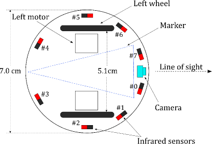
Figure 16: Schematic top view of an e-puck, indicating the locations of its motors, wheels, camera and infrared sensors. Note that the marker is pointing towards the robot’s back.

A schematic top view of the e-puck is shown in Fig. 16. We implement the line-of-sight sensor using the e-puck’s directional camera, located at its front. For this purpose, we wrap the robots in black ‘skirts’ (see Fig. 1) to make them distinguishable against the light-colored arena. While in principle the sensor could be implemented using one pixel, we use a column of pixels from a subsampled image to compensate for misalignment in the camera’s vertical orientation. The gray values from these pixels are used to distinguish robots ($I=1$) against the arena ($I=0$). For more details about this sensor realization, see (Gauci et al., 2014c).

We also use the e-puck’s infrared sensors, in two cases. Firstly, before each trial, the robots disperse themselves within the arena. In this case, they use the infrared sensors to avoid both robots and walls, making the dispersion process more efficient. Secondly, we observe that using only the line-of-sight sensor can lead to robots becoming stuck against the walls of the arena, hindering the identification process. We therefore use the infrared sensors for wall avoidance, but in such a way as to not affect inter-robot interactions. Details of these two collision avoidance behaviors are provided in the online supplementary materials (Li et al., 2016).

5.1.3 Motion capture

To facilitate motion data extraction, we fit robots with markers on their tops, consisting of a colored isosceles triangle on a circular white background (see Fig. 1). The triangle’s color allows for distinction between robots; we use blue triangles for all agents, and orange and purple triangles for the two replicas. The triangle’s shape eases extraction of robots’ orientations.

The robots’ motion is captured using a camera mounted around $270\,\mathrm{cm}$ above the arena floor. The camera’s frame rate is set to $10\,\mathrm{fps}$. The video stream is fed to the PC, which performs video processing to extract motion data about individual robots (position and orientation). The video processing software is written using OpenCV (Bradski and Kaehler, 2008).

5.2 Turing Learning with physical robots

Our objective is to infer the agent’s aggregation behavior. We do not wish to infer the agent’s dispersion behavior, which is periodically executed to distribute already-aggregated agents. To separate these two behaviors, the robots (agents and replicas) and the system are implicitly synchronized. This is realized by making each robot execute a fixed behavioral loop of constant duration. The PC also executes a fixed behavioral loop, but the timing is determined by the signals received from the replicas. Therefore, the PC is synchronized with the swarm. The PC communicates with the replicas via Bluetooth. At the start of a run, or after a human intervention (see Section 5.3), robots are initially synchronized using an infrared signal from a remote control.

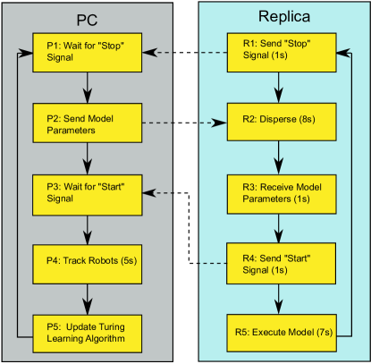
Figure 17: Flow diagram of the programs run by the PC and a replica in the physical experiments. Dashed arrows represent communication between the two units. See Section 5.2 for details. The PC does not exert any control over the agents.

Fig. 17 shows a flow diagram of the programs run by the PC and the replicas, respectively. Dashed arrows indicate communication between the units.

The program running on the PC has the following states:

• P1. Wait for “Stop” Signal. The program is paused until “Stop” signals are received from both replicas. These signals indicate that a trial has finished.

• P2. Send Model Parameters. The PC sends new model parameters to the buffer of each replica.

• P3. Wait for “Start” Signal. The program is paused until “Start” signals are received from both replicas, indicating that a trial is starting.

• P4. Track Robots. The PC waits $1\,\mathrm{s}$ and then tracks the robots using the overhead camera for $5\,\mathrm{s}$. The tracking data contain the positions and orientations of the agents and replicas.

• P5. Update Turing Learning Algorithm. The PC uses the motion data from the trial observed in P4 to update the solution quality (fitness values) of the corresponding two models and all classifiers. Once all models in the current iteration cycle (generation) have been evaluated, the PC also generates new model and classifier populations. The method for calculating the qualities of solutions and the optimization algorithm are described in Sections 3.1 and 3.2.4 respectively. The PC then goes back to P1.

The program running on the replicas has the following states:

• R1. Send “Stop” Signal. After a trial stops, the replica informs the PC by sending a “Stop” signal. The replica waits $1\,\mathrm{s}$ before proceeding with R2, so that all robots remain synchronized. Waiting $1\,\mathrm{s}$ in other states serves the same purpose.

• R2. Disperse. The replica disperses in the environment, while avoiding collisions with other robots and the walls. This behavior lasts $8\,\mathrm{s}$.

• R3. Receive Model Parameters. The replica reads new model parameters from its buffer (sent earlier by the PC). It waits $1\,\mathrm{s}$ before proceeding with R4.

• R4. Send “Start” Signal. The replica sends a start signal to the PC to inform it that a trial is about to start. The replica waits $1\,\mathrm{s}$ before proceeding with R5.

• R5. Execute Model. The replica moves within the swarm according to its model. This behavior lasts $7\,\mathrm{s}$ (the tracking data corresponds to the middle $5\,\mathrm{s}$, see P4). The replica then goes back to R1.

The program running on the agents has the same structure as the replica program. However, in the states analogous to R1, R3, and R4, they simply wait $1\,\mathrm{s}$ rather than communicate with the PC. In the state corresponding to R2, they also execute the Disperse behavior. In the state corresponding to R5, they execute the agent’s aggregation controller, rather than a model.

Each iteration (loop) of the program for the PC, replicas and agents lasts $18\,\mathrm{s}$.

5.3 Experimental setup

As in simulation, we use a population size of $100$ for classifiers ($\mu=50$, $\lambda=50$). However, the model population size is reduced from $100$ to $20$ ($\mu=10$, $\lambda=10$), to shorten the experimentation time. We use $10$ robots: $8$ representing agents executing the original aggregation controller (Eq. (6)), and $2$ representing replicas that execute models. This means that in each trial, $2$ models from the population could be simultaneously evaluated; consequently, each generation consists of $20/2=10$ trials.

The Turing Learning algorithm is implemented without any modification to the code used in simulation (except for model population size and observation time in each trial). We still let the model parameters evolve unboundedly (i.e., in $\mathbb{R}^{4}$). However, as the speed of the physical robots is naturally bounded, we apply the hyperbolic tangent function ($\tanh{x}$) on each model parameter, before sending a model to a replica. This bounds the parameters to $\left(-1,1\right)^{4}$, with $-1$ and $1$ representing the maximum backwards and forwards wheel speeds, respectively.

The Turing Learning runs proceed autonomously. In the following cases, however, there is intervention:

• The robots have been running continuously for $25$ generations. All batteries are replaced.

• Hardware failure has occurred on a robot, for example because of a lost battery connection or because the robot has become stuck on the floor. Appropriate action is taken for the affected robot to restore its functionality.

• A replica has lost its Bluetooth connection with the PC. The connection with both replicas is restarted.

• A robot indicates a low battery status through its LED after running for only a short time. That robot’s battery is changed.

After an intervention, the ongoing generation is restarted, to limit the impact on the identification process.

We conducted $10$ runs of Turing Learning using the physical system. Each run lasted $100$ generations, corresponding to $5$ hours (excluding human intervention time). Video recordings of all runs can be found in the online supplementary materials (Li et al., 2016).

5.4 Analysis of inferred models

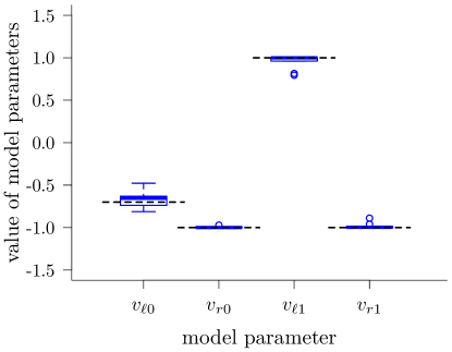
Figure 18: Model parameters Turing Learning inferred from swarms of physical robots performing aggregation. The models are those with the highest subjective fitness in the $100$th generation of $10$ runs. Dashed black lines indicate the ground truth, that is, the values of the parameters that the system is expected to learn.

We first investigate the quality of the models obtained. To select the ‘best’ model from each run, we post-evaluated all models of the final generation $5$ times using all classifiers of that generation. The parameters of these models are shown in Fig. 18. The means (standard deviations) of the AEs in each parameter are as follows: $0.08$ ($0.06$), $0.01$ ($0.01$), $0.05$ ($0.08$), and $0.02$ ($0.04$).

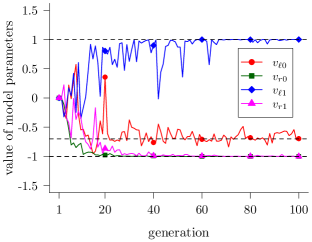
(a) (a) physical coevolutions

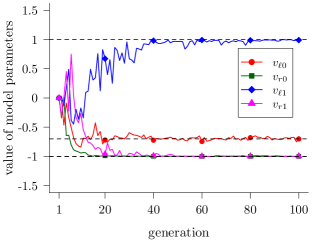
(b) (b) simulated coevolutions

Figure 19: Evolutionary dynamics of model parameters in (a) $10$ physical and (b) $10$ simulated runs of Turing Learning (in both cases, equivalent setups were used). Curves represent median parameter values of the models with the highest subjective fitness across the $10$ runs. Dashed black lines indicate the ground truth.

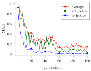
(a) (a) physical coevolutions

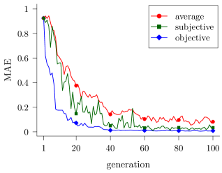
(b) (b) simulated coevolutions

Figure 20: Evolutionary dynamics of MAE (defined in Eq. (10)) for the candidate models in (a) $10$ physical and (b) $10$ simulated runs of Turing Learning. Curves represent median values across $10$ runs. The red curve represents the average error of all models in a generation. The green and blue curves show, respectively, the errors of the models with the highest subjective and the highest objective fitness in a generation.

To investigate the effects of real-world conditions on the identification process, we performed $10$ simulated runs of Turing Learning with the same setup as in the physical runs. Fig. 19 shows the evolutionary dynamics of the parameters of the inferred models (with the highest subjective fitness) in the physical and simulated runs. The dynamics show good correspondence. However, the convergence in the physical runs is somewhat less smooth than that in the simulated ones (e.g., see spikes in $v_{\ell 0}$ and $v_{\ell 1}$). In each generation of every run (physical and simulated), we computed the MAE of each model. We compared the error of the model with the highest subjective fitness with the average and lowest errors. The results are shown in Fig. 20. For both the physical and simulated runs, the subjectively best model (green) has an error in between the lowest error (blue) and the average error (red) in the majority of generations.

As we argued before (Section 4.3), in swarm systems, good agreement between local behaviors (e.g., controller parameters) may not guarantee similar global behaviors. For this reason, we investigate both the original controller (Eq. (6)), and a controller obtained from the physical runs. This latter controller is constructed by taking the median values of the parameters over the $10$ runs, which are:

$$\mathbf{p}=\left(-0.65,-0.99,0.99,-0.99\right).$$

The set of initial configurations of the robots is common to both controllers. As it is not necessary to extract the orientation of the robots, a red circular marker is attached to each robot so that its position can be extracted with higher accuracy in the offline analysis (Gauci et al., 2014c).

(a) (a) Largest Cluster Dynamics

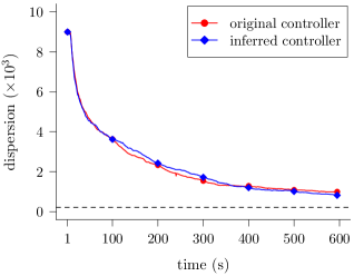
(b) (b) Dispersion Dynamics

Figure 21: Average aggregation dynamics in $10$ physical trials with $40$ physical e-puck robots executing the original agent controller (red) and the model controller (blue) inferred through observation of the physical system. In (a), the vertical axis shows the proportion of robots in the largest cluster; in (b), it shows the robots’ dispersion (see Section 4.3). Dashed lines in (a) and (b) respectively represent the maximum proportion and minimum dispersion that $40$ robots can achieve.

(a) initial configuration

(b) after $20$ $\mathrm{s}$

(c) after $40$ $\mathrm{s}$

(d) after $180$ $\mathrm{s}$

(e) after $360$ $\mathrm{s}$

(f) after $420$ $\mathrm{s}$

(g) after $480$ $\mathrm{s}$

(h) after $600$ $\mathrm{s}$

Figure 22: Example of collective behavior produced by a model that was inferred by Turing Learning through the observation of swarms of physical e-puck robots. A swarm of $40$ physical e-puck robots, each executing the inferred model, aggregates in a single spot.

For each controllers, we performed $10$ trials using $40$ physical e-pucks. Each trial lasted $10$ minutes. Fig. LABEL:sub@fig:aggregation_dynamics_proportion shows the proportion of robots in the largest cluster over time with the agent and model controllers. Fig. LABEL:sub@fig:aggregation_dynamics_compactness shows the dispersion (as defined in Section 4.3) of the robots over time with the two controllers. The aggregation dynamics of the agents and the models show good correspondence. Fig. 22 shows a sequence of snapshots from a trial with $40$ e-pucks executing the inferred model controller.

A video accompanying this paper shows the Turing Learning identification process of the models (in a particular run) both in simulation and on the physical system. Additionally, videos of all $20$ post-evaluation trials with $40$ e-pucks, are provided in the online supplementary materials (Li et al., 2016).

5.5 Analysis of generated classifiers

Figure 23: Average decision accuracy of the best classifiers over $100$ generations (nonlinear scale) in $10$ runs of Turing Learning with swarms of physical robots. Average over 100 data samples from a post-evaluation with physical robots executing random models. The error bars show standard deviations. See text for details.

When post-evaluating the classifiers generated in the physical runs of Turing Learning, we limited the number of candidate models to $100$, in order to reduce the physical experimentation time. Each candidate model was chosen randomly, with uniform distribution, from the parameter space defined in Eq. (5). Fig. 23 shows the average decision accuracy of the best classifiers over the $10$ runs. Similar to the results in simulation, the best classifier (objective) still has a high decision accuracy. However, in contrast to simulation, the decision accuracy of the best classifier (subjective) does not drop within $100$ generations. This could be due to the noise present in the physical runs, which may have prevented the classifiers from getting over-specialized in the comparatively short time provided (100 generations).

6 Conclusions

This paper presented a new system identification method—Turing Learning—that can autonomously infer the behavior of a system from observations. To the best of our knowledge, Turing Learning is the first system identification method that does not rely on any predefined metric to quantitatively gauge the difference between the system and the inferred models. This eliminates the need to choose a suitable metric and the bias that such metric may have on the identification process.

Through competitive and successive generation of models and classifiers, the system successfully learned two behaviors: self-organized aggregation and object clustering in swarms of mobile agents. Both the model parameters, which were automatically inferred, and emergent global behaviors closely matched those of the original swarm system.

We also examined a conventional system identification method, which used a least-square error metric rather than classifiers. We proved that the metric-based method was fundamentally flawed for the case studies considered here. In particular, as the inputs to the agents and to the models were not correlated, the model solution that was globally optimal with respect to the metric was not identical to the agent solution. In other words, according to the metric, the parameter set of the agent itself scored worse than a different—and hence incorrect—parameter set. Simulation results were in good agreement with these theoretical findings.

The classifiers generated by Turing Learning can be a useful by-product. Given a data sample (motion trajectory), they can tell whether it is genuine, in other words, whether it originates from the reference system. Such classifiers could be used for detecting abnormal behavior,—for example when faults occur in some members of the swarm—and are obtained without the need to define a priori what constitutes abnormal behavior.

In this paper, we presented the main results using a gray box model representation; in other words, the model structure was assumed to be known. Consequently, the inferred model parameters could be compared against the ground truth, enabling us to objectively gauge the quality of the identification process. Note that even though the search space for the models is small, identifying the parameters is challenging as the input values are unknown (consequently, the metric-based system identification method did not succeed in this respect).

The Turing Learning method was further validated using a physical system. We applied it to automatically infer the aggregation behavior of an observed swarm of e-puck robots. The behavior was learned successfully, and the results obtained in the physical experiments showed good correspondence with those obtained in simulation. This shows the robustness of our method with respect to noise and uncertainties typical of real-world experiments. To the best of our knowledge, this is also the first time that a system identification method was used to infer the behavior of physical robots in a swarm.

We conducted further simulation experiments to test the generality of Turing Learning. First, we showed that Turing Learning can simultaneously infer the agent’s brain (controller) as well as an aspect of the agent’s morphology that determines its field of view. Second, we showed that Turing Learning can infer the behavior without assuming the agent’s control system structure to be known. The models were represented as fixed-structure recurrent neural networks, and the behavior could still be successfully inferred. For more complex behaviors, one could adopt other optimization algorithms such as NEAT (Stanley and Miikkulainen, 2002), which gradually increases the complexity of the neural networks being evolved. Third, we assessed an alternative setup of Turing Learning, in which the replica—the robot used to test the models—is not in the same environment as the swarm of agents. While this requires a swarm of replicas, it has the advantage of ensuring that the agents are not affected by the replica’s presence. In addition, it opens up the possibility of the replica not being a physical agent, but rather residing in a simulated world, which may lead to a less costly implementation. On the other hand, the advantage of using a physical replica is that it may help to address the reality gap issue. As the replica shares the same physics as the agent, its evolved behavior will rely on the same physics. This is not necessarily true for a simulated replica—for instance, when evolving a simulated fish it is hard (and computationally expensive) to fully capture the hydrodynamics of the real environment. As a final experiment, we showed that Turing Learning is able to infer a wide range of randomly generated reactive behaviors.

In the future, we intend to use Turing Learning to infer the complex behaviors exhibited in natural swarms, such as in shoals of fish or herds of land mammals. We are interested in both reactive and non-reactive behaviors. As shown in (Li et al., 2013; Li, 2016), it can be beneficial if the classifiers are not restricted to observing the system passively. Rather, they could influence the process by which data samples are obtained, effectively choosing the conditions under which the system is to be observed.

References

- Arkin (1998) Arkin, R.C. (1998). Behavior-based robotics. MIT Press, Cambridge, MA.
- Billings (2013) Billings, S.A. (2013). Nonlinear system identification: NARMAX methods in the time, frequency, and spatio-temporal domains. Wiley, Hoboken, NJ.
- Bjerknes and Winfield (2013) Bjerknes, J. and Winfield, A.F.T. (2013). On fault tolerance and scalability of swarm robotic systems. In A. Martinoli, F. Mondada, N. Correll, G. Mermoud, M. Egerstedt, A.M. Hsieh, et al. (eds.), Distributed Autonomous Robotic Systems, volume 83, 431–444. Springer, Berlin, Heidelberg.
- Bongard and Lipson (2004a) Bongard, J. and Lipson, H. (2004a). Automated damage diagnosis and recovery for remote robotics. In Proceedings of the 2004 IEEE International Conference on Robotics and Automation, 3545–3550. IEEE, Piscataway, NJ.
- Bongard and Lipson (2004b) Bongard, J. and Lipson, H. (2004b). Automated robot function recovery after unanticipated failure or environmental change using a minimum of hardware trials. In Proceedings of the 2004 NASA/DoD Conference on Evolvable Hardware, 169–176. IEEE, Piscataway, NJ.
- Bongard and Lipson (2005) Bongard, J. and Lipson, H. (2005). Nonlinear system identification using coevolution of models and tests. IEEE Transactions on Evolutionary Computation, 9(4), 361–384.
- Bongard et al. (2006) Bongard, J., Zykov, V., and Lipson, H. (2006). Resilient machines through continuous self-modeling. Science, 314(5802), 1118–1121.
- Bongard and Lipson (2007) Bongard, J. and Lipson, H. (2007). Automated reverse engineering of nonlinear dynamical systems. Proceedings of the National Academy of Sciences, 104(24), 9943–9948.
- Bradski and Kaehler (2008) Bradski, G. and Kaehler, A. (2008). Learning OpenCV: Computer vision with the OpenCV library. O’Reilly Media, Sebastopol, CA.
- Braitenberg (1984) Braitenberg, V. (1984). Vehicles: Experiments in synthetic psychology. MIT Press, Cambridge, MA.
- Brooks (1991) Brooks, R.A. (1991). Intelligence without representation. Artificial Intelligence, 47(1), 139–159.
- Camazine et al. (2003) Camazine, S., Deneubourg, J.L., Franks, N.R., Sneyd, J., Theraula, G., and Bonabeau, E. (2003). Self-Organization in Biological Systems. Princeton University Press, Princeton, NJ.
- Cully et al. (2015) Cully, A., Clune, J., Tarapore, D., and Mouret, J. (2015). Robots that can adapt like animals. Nature, 521(7553), 503–507.
- Eiben and Smith (2003) Eiben, A.E. and Smith, J.E. (2003). Introduction to Evolutionary Computing. Springer, Berlin, Heidelberg.
- Elman (1990) Elman, J.L. (1990). Finding structure in time. Cognitive Science, 14(2), 179–211.
- Faria et al. (2010) Faria, J.J., Dyer, J.R.G., Clément, R.O., Couzin, I.D., Holt, N., Ward, A.J.W., et al. (2010). A novel method for investigating the collective behaviour of fish: Introducing ‘Robofish’. Behavioral Ecology and Sociobiology, 64(8), 1211–1218.
- Floreano and Mondada (1996) Floreano, D. and Mondada, F. (1996). Evolution of homing navigation in a real mobile robot. IEEE Transactions on Systems, Man, and Cybernetics, Part B, 26(3), 396–407.
- Gauci et al. (2014a) Gauci, M., Chen, J., Dodd, T., and Groß, R. (2014a). Evolving aggregation behaviors in multi-robot systems with binary sensors. In M. Ani Hsieh and G. Chirikjian (eds.), Distributed Autonomous Robotic Systems, volume 104, 355–367. Springer, Berlin, Heidelberg.
- Gauci et al. (2014b) Gauci, M., Chen, J., Li, W., Dodd, T.J., and Groß, R. (2014b). Clustering objects with robots that do not compute. In Proceedings of the 2014 Internation Conference Autonomous Agents and Multi-Agent Systems, 421–428. IFAAMAS, Richland, SC.
- Gauci et al. (2014c) Gauci, M., Chen, J., Li, W., Dodd, T.J., and Groß, R. (2014c). Self-organized aggregation without computation. International Journal of Robotics Research, 33(8), 1145–1161.
- Goodfellow et al. (2014) Goodfellow, I. et al. (2014). Generative adversarial nets. In Z. Ghahramani, M. Welling, C. Cortes, N.D. Lawrence, and K.Q. Weinberger (eds.), Advances in Neural Information Processing Systems, 2672–2680. Curran Associates, Inc.
- Graham and Sloane (1990) Graham, R.L. and Sloane, N.J.A. (1990). Penny-packing and two-dimensional codes. Discrete and Computational Geometry, 5(1), 1–11.
- Halloy et al. (2007) Halloy, J., Sempo, G., Caprari, G., Rivault, C., Asadpour, M., Tâche, F., et al. (2007). Social integration of robots into groups of cockroaches to control self-organized choices. Science, 318(5853), 1155–1158.
- Halloy et al. (2013) Halloy, J., Mondada, F., Kernbach, S., and Schmickl, T. (2013). Towards bio-hybrid systems made of social animals and robots. In N.F. Lepora, A. Mura, H.G. Krapp, P. Verschure, and T.J. Prescott (eds.), Biomimetic and Biohybrid Systems, volume 8064, 384–386. Springer, Berlin, Heidelberg.
- Harel (2005) Harel, D. (2005). A Turing-like test for biological modeling. Nature Biotechnology, 23, 495–496.
- Harnad (2000) Harnad, S. (2000). Minds, machines and Turing: The indistinguishability of indistinguishables. Journal of Logic, Language and Information, 9(4), 425–445.
- Harvey et al. (2015) Harvey, J., Merrick, K., and Abbass, H.A. (2015). Application of chaos measures to a simplified boids flocking model. Swarm Intelligence, 9(1), 23–41.
- Heinerman et al. (2015) Heinerman, J., Rango, M., and Eiben, A.E. (2015). Evolution, individual learning, and social learning in a swarm of real robots. In Proceedings of the 2015 Genetic and Evolutionary Computation Conference, 177–183. ACM, New York, NY.
- Helbing and Johansson (2011) Helbing, D. and Johansson, A. (2011). Pedestrian, crowd and evacuation dynamics. In R.A. Meyers (ed.), Extreme Environmental Events, 697–716. Springer, New York, NY.
- Herbert-Read et al. (2015) Herbert-Read, J.E., Romenskyy, M., and Sumpter, D.J.T. (2015). A Turing test for collective motion. Biology Letters, 11(12), 20150674.
- Jakobi et al. (1995) Jakobi, N., Husbands, P., and Harvey, I. (1995). Noise and the reality gap: The use of simulation in evolutionary robotics. In F. Morán, A. Moreno, J. Merelo, and P. Chacón (eds.), Advances in Artificial Life, volume 929, 704–720. Springer, Berlin, Heidelberg.
- Koos et al. (2009) Koos, S., Mouret, J., and Doncieux, S. (2009). Automatic system identification based on coevolution of models and tests. In Proceedings of the 2009 IEEE Congress on Evolutionary Computation, 560–567. IEEE, Piscataway, NJ.
- Koos et al. (2013) Koos, S., Mouret, J., and Doncieux, S. (2013). The transferability approach: Crossing the reality gap in evolutionary robotics. IEEE Transactions on Evolutionary Computation, 17(1), 122–145.
- Krause et al. (2011) Krause, J., Winfield, A.F., and Deneubourg, J.L. (2011). Interactive robots in experimental biology. Trends in Ecology and Evolution, 26(7), 369–375.
- Le Ly and Lipson (2014) Le Ly, D. and Lipson, H. (2014). Optimal experiment design for coevolutionary active learning. IEEE Transactions on Evolutionary Computation, 18(3), 394–404.
- Levi and Kernbach (2010) Levi, P. and Kernbach, S. (2010). Symbiotic multi-robot organisms: Reliability, adaptability, evolution. Springer, Berlin, Heidelberg.
- Li et al. (2013) Li, W., Gauci, M., and Groß, R. (2013). A coevolutionary approach to learn animal behavior through controlled interaction. In Proceedings of the 2013 Genetic and Evolutionary Computation, 223–230. ACM, New York, NY.
- Li et al. (2014) Li, W., Gauci, M., and Groß, R. (2014). Coevolutionary learning of swarm behaviors without metrics. In Proceedings of the 2014 Genetic and Evolutionary Computation Conference, 201–208. ACM, New York, NY.
- Li (2016) Li, W. (2016). Automated reverse engineering of agent behaviors. Ph.D. thesis, The University of Sheffield. URL http://etheses.whiterose.ac.uk/12375/.
- Li et al. (2016) Li, W., Gauci, M., and Groß, R. (2016). Online supplementary material. URL http://naturalrobotics.group.shef.ac.uk/supp/2016-003.
- Ljung (2010) Ljung, L. (2010). Perspectives on system identification. Annual Reviews in Control, 34(1), 1–12.
- Magnenat et al. (2011) Magnenat, S., Waibel, M., and Beyeler, A. (2011). Enki: The fast 2D robot simulator. URL http://home.gna.org/enki.
- Mirmomeni and Punch (2011) Mirmomeni, M. and Punch, W. (2011). Co-evolving data driven models and test data sets with the application to forecast chaotic time series. In Proceedings of the 2011 IEEE Congress on Evolutionary Computation, 14–20. IEEE, Piscataway, NJ.
- Mondada et al. (2009) Mondada, F., Bonani, M., Raemy, X., Pugh, J., Cianci, C., Klaptocz, A., et al. (2009). The e-puck, a robot designed for education in engineering. In Proceedings of the 9th Conference on Autonomous Robot Systems and Competitions, 59–65. IEEE, Bragança, Portugal.
- Nguyen et al. (2015) Nguyen, A., Yosinski, J., and Clune, J. (2015). Deep neural networks are easily fooled: High confidence predictions for unrecognizable images. In Proceedings of the 2015 IEEE Conference on Computer Vision and Pattern Recognition, 427–436. IEEE, Boston, MA.
- O’Dowd et al. (2014) O’Dowd, P.J., Studley, M., and Winfield, A.F. (2014). The distributed co-evolution of an on-board simulator and controller for swarm robot behaviours. Evolutionary Intelligence, 7(2), 95–106.
- Radford et al. (2016) Radford, A., Metz, L., and Chintala, S. (2016). Unsupervised representation learning with deep convolutional generative adversarial networks. In Proceedings of the 2016 International Conference on Learning Representations. In press; available online: http://arxiv.org/abs/1511.06434.
- Saygin et al. (2000) Saygin, A.P., Cicekli, I., and Akman, V. (2000). Turing test: 50 years later. Minds and Machines, 10, 463–518.
- Schmickl et al. (2013) Schmickl, T., Bogdan, S., Correia, L., Kernbach, S., Mondada, F., Bodi, M., et al. (2013). Assisi: Mixing animals with robots in a hybrid society. In N.F. Lepora, A. Mura, H.G. Krapp, P. Verschure, and T.J. Prescott (eds.), Biomimetic and Biohybrid Systems, 441–443. Springer, Berlin, Heidelberg.
- Stanley and Miikkulainen (2002) Stanley, K.O. and Miikkulainen, R. (2002). Evolving neural networks through augmenting topologies. Evolutionary Computation, 10(2), 99–127.
- Turing (1950) Turing, A.M. (1950). Computing machinery and intelligence. Mind, 59(236), 433–460.
- Vaughan et al. (2000) Vaughan, R., Sumpter, N., Henderson, J., Frost, A., and Stephen, C. (2000). Experiments in automatic flock control. Robot. Auton. Syst., 31(1), 109–117.
- Watson et al. (2002) Watson, R.A., Ficici, S.G., and Pollack, J.B. (2002). Embodied evolution: Distributing an evolutionary algorithm in a population of robots. Robotics and Autonomous Systems, 39(1), 1–18.
- Weitz et al. (2012) Weitz, S., Blanco, S., Fournier, R., Gautrais, J., Jost, C., and Theraulaz, G. (2012). Modeling collective animal behavior with a cognitive perspective: A methodological framework. PLoS ONE, 7(6), e38588.
- Zykov et al. (2004) Zykov, V., Bongard, J., and Lipson, H. (2004). Evolving dynamic gaits on a physical robot. In Proceedings of the 2004 Genetic and Evolutionary Computation Conference, 4722–4728. ACM, New York, NY.