RADIO POLARIZATION OBSERVATIONS OF THE SNAIL: A CRUSHED PULSAR WIND NEBULA IN G327.1$-$1.1 WITH A HIGHLY ORDERED MAGNETIC FIELD

Abstract

Pulsar wind nebulae (PWNe) are suggested to be acceleration sites of cosmic rays in the Galaxy. While the magnetic field plays an important role in the acceleration process, previous observations of magnetic field configurations of PWNe are rare, particularly for evolved systems. We present a radio polarization study of the “Snail” PWN inside the supernova remnant G327.1$-$1.1 using the Australia Telescope Compact Array. This PWN is believed to have been recently crushed by the supernova (SN) reverse shock. The radio morphology is composed of a main circular body with a finger-like protrusion. We detected a strong linear polarization signal from the emission, which reflects a highly ordered magnetic field in the PWN and is in contrast to the turbulent environment with a tangled magnetic field generally expected from hydrodynamical simulations. This could suggest that the characteristic turbulence scale is larger than the radio beam size. We built a toy model to explore this possibility, and found that a simulated PWN with a turbulence scale of about one-eighth to one-sixth of the nebula radius and a pulsar wind filling factor of 50–75% provides the best match to observations. This implies substantial mixing between the SN ejecta and pulsar wind material in this system.

1. INTRODUCTION

A massive star ends its life as a supernova (SN) explosion. This leaves behind a supernova remnant (SNR) and sometimes creates a rapidly rotating pulsar. A pulsar can produce an outflow of a magnetic field and relativistic particles referred to as a pulsar wind. The interaction between such a pulsar wind and the ambient medium, i.e. the SN ejecta for pulsars embedded in SNRs, results in a termination shock, beyond which the shocked wind materials inflate a broadband synchrotron-emitting bubble known as a pulsar wind nebula (PWN).

The evolution of PWNe can be divided into several stages (see Blondin et al., 2001; van der Swaluw et al., 2001, 2004; Gelfand et al., 2009). A PWN first expands supersonically inside its associated SNR. The next stage starts when the SN reverse shock, which is driven inward by the interaction between the ejecta and the interstellar medium, crushes the PWN. The interplay between the shockwave and the PWN is complex and will cause the PWN to reverberate (e.g. van der Swaluw et al., 2001). After the effect of the reverse shock fades away, the PWN will expand subsonically into the SNR. Since a pulsar is generally born with high space velocity, it can be significantly off-centered with respect to the SNR during the reverberation stage and can protrude from its own PWN because of the reverse shock interaction (van der Swaluw et al., 2004). This can result in a complicated PWN morphology consisting of a “relic” component and an elongated “head” bridging between the relic and the pulsar (van der Swaluw et al., 2004). As the pulsar continues to travel toward the edge of the SNR, its motion will eventually become supersonic because the local sound speed in an SNR decreases moving outward. The ram pressure acting on the pulsar wind due to the pulsar’s supersonic motion will deform the PWN into a bow shock. For even older systems, the pulsar can escape from its associated SNR shell and drive a bow-shock PWN into the interstellar medium.

Broadband emission from PWNe can be observed from the radio to $\gamma$-rays. In the radio regime, a PWN emits through the synchrotron process, and the emission is often highly linear polarized because of the ordered magnetic field configuration. A radio PWN is characterized by a centrally filled morphology and a flat spectrum, with a spectral index of $-0.3\leq\alpha\leq 0$ ($S_{\nu}\propto\nu^{\alpha}$). The synchrotron spectrum can extend to the X-ray band where the spectrum is usually steeper than that in the radio due to synchrotron cooling. GeV and TeV $\gamma$-ray emission from PWNe has also been detected, which is due to inverse-Compton scattering (see the review by Gaensler & Slane, 2006).

One interesting area to explore in the study of PWNe is the interaction with the SN reverse shocks. Theoretically, hydrodynamical (HD) modeling shows that the interplay can give rise to turbulence in PWNe (Blondin et al., 2001; van der Swaluw et al., 2004). However, the role of the magnetic field is unclear since magnetohydrodynamic (MHD) efforts are lacking. Observationally, we aim to probe the magnetic field structure of these PWNe to expand the currently inadequate sample size. The results from our study can serve as inputs to MHD modeling.

One of the few examples of such systems is G327.1$-$1.1 (catalog ), which is an SNR system containing a PWN that is believed to have been recently crushed by the reverse shock. It was discovered as a non-thermal radio source (Clark et al., 1973, 1975). Its peculiar radio morphology was revealed by the Molonglo Observatory Synthesis Telescope (MOST) SNR survey (Whiteoak & Green, 1996). The SNR shell is $17^{\prime}$ in diameter and contains an off-centered PWN. The latter consists of a circular main body with a $3^{\prime}$ diameter together with a $2^{\prime}$-long finger-like structure protruding northwest from the main body.

The first X-ray detection of G327.1$-$1.1 was reported by Lamb & Markert (1981) using the Einstein Observatory. Further X-ray studies were conducted with ROSAT (Seward et al., 1996; Sun et al., 1999), ASCA (Sun et al., 1999), BeppoSAX (Bocchino & Bandiera, 2003), Chandra (Temim et al., 2009, 2015), and XMM-Newton (Temim et al., 2009). The X-ray remnant consists of a diffuse thermal component covering the radio shell and a non-thermal component coinciding with the radio PWN. An X-ray compact source at the tip of the finger was discovered along with two prong-like structures extending northwest from the finger into a diffuse, arc-like structure (Temim et al., 2009, 2015). The compact source is interpreted as the neutron star powering the PWN, but the nature of the prongs and the arc is not well understood. Sun et al. (1999) estimated the distance to G327.1$-$1.1 to be $d=9.0\,{\rm kpc}$ based on an empirical relationship between the X-ray column density $N_{\rm H}$ and the color excess $E(B-V)$, and the observed relationship between $E(B-V)$ and the distance $d$ along the line of sight to G327.1$-$1.1. We will adopt this number ($d=9.0\,{\rm kpc}$) in our analysis.

In $\gamma$-rays, a preliminary report of TeV detection of G327.1$-$1.1 with H.E.S.S. was described by Acero et al. (2012). As the photon index in TeV was found to be similar to that in keV, they suggested that the emission in the two bands could originate from the same population of particles through inverse-Compton and synchrotron processes, respectively. This source has not been detected in the GeV range by Fermi LAT (Acero et al., 2013, 2015).

By considering the current position of the presumed neutron star relative to the SN shell, Temim et al. (2009) suggested that the neutron star is moving northward. The main body of the PWN is interpreted as the relic, and the overall PWN morphology could be caused by the reverse shock first crushing the PWN from the northwest, thus pushing the relic to the southeast. The asymmetry of the reverse shock interaction is attributed to both the inhomogeneous ambient interstellar medium and the pulsar’s motion. This picture is supported by recent HD simulations (Temim et al., 2015). It is believed that the PWN has not yet evolved into the bow-shock stage (van der Swaluw et al., 2004; Temim et al., 2009, 2015).

In this paper, we present radio observations of the PWN in G327.1$-$1.1 with the Australia Telescope Compact Array (ATCA). We obtained polarimetric measurements at 6 and 3 cm to investigate the magnetic field structure of the PWN. The observations and data reduction procedures are described in Section 2. We show the results in Section 3 and discuss our findings in Section 4. We close by summarizing our work in Section 5.

2. OBSERVATIONS AND DATA REDUCTION

Radio observations of the PWN in G327.1$-$1.1 were performed with ATCA at 6 and 3 cm on 2008 December 09 and 2009 February 19 with array configurations of 750B and EW352, respectively. The observation parameters are listed in Table 1. All of the observations were carried out prior to the Compact Array Broadband Backend (CABB) upgrade (Wilson et al., 2011). The data were taken in continuum mode with all four Stokes parameters recorded over a usable bandwidth of 104 MHz at each frequency. We observed for a total integration time of $20.8\,{\rm hr}$ in each band as a five-pointing mosaic. PKS B1934$-$638 was adopted as the primary calibrator to set the flux density scale, and PKS 1613$-$586 was observed at 20 minute intervals to determine the antenna gain solution. We also processed archival ATCA pre-CABB data at 20 and 13 cm, for which the observation parameters are also listed in Table 1. The 13 cm observations were performed in continuum mode with the same usable bandwidth of 104 MHz. However, the 20 cm observations were performed in spectral line mode on the H i line, such that only the total intensity (i.e. no polarization) within a narrow usable bandwidth of 4 MHz was recorded. The simultaneous observations at 20 and 13 cm consist of a single pointing at G327.1$-$1.1, with array configurations of 1.5D and 750D for a total integration time of $19.0\,{\rm hr}$ per band. PKS B1934$-$638 was also used as the primary calibrator for these two bands, and PKS 1610$-$771 was observed every 45 minutes for antenna gain calibration.

Table 1ATCA Observation Parameters of the Snail

Obs. Date	Array Config.	Center Freq.	Usable Bandwidth	No. of	Integration
		(MHz)	(MHz)	Channels	Time (hr)
2000 Apr 17	1.5D	1420, 2496	4, 104	1025, 13	9.1
2000 Apr 29	750D	1420, 2240	4, 104	1025, 13	9.9
2008 Dec 09	750B	4800, 8640	104, 104	13, 13	10.4
2009 Feb 19	EW352	4800, 8640	104, 104	13, 13	10.4

Table 2Flux Densities and Spectral Indices of Different Parts of the Snail

$\lambda$ (cm)	Whole PWN	The Body	The Head
36	$2.3\pm 0.2\,{\rm Jy}$	$2.1\pm 0.1\,{\rm Jy}$	$0.18\pm 0.02\,{\rm Jy}$
20	$2.1\pm 0.4\,{\rm Jy}$	$1.8\pm 0.4\,{\rm Jy}$	$0.30\pm 0.06\,{\rm Jy}$
13	$1.8\pm 0.3\,{\rm Jy}$	$1.5\pm 0.2\,{\rm Jy}$	$0.23\pm 0.03\,{\rm Jy}$
6	$1.5\pm 0.2\,{\rm Jy}$	$1.3\pm 0.1\,{\rm Jy}$	$0.16\pm 0.02\,{\rm Jy}$
3	$0.94\pm 0.06\,{\rm Jy}$	$0.83\pm 0.06\,{\rm Jy}$	$0.11\pm 0.01\,{\rm Jy}$
$\alpha$ ($S_{\nu}\propto\nu^{\alpha}$)	$-0.3\pm 0.1$	$-0.3\pm 0.1$	$-0.6\pm 0.1$

We used the MIRIAD package (Sault et al., 1995) for all of the data reduction. First, edge channels and channels known to be affected by radio frequency interference were discarded. We then examined the data and flagged bad data points during periods of poor atmospheric stability. Next, bandpass, gain, polarization, and flux calibration solutions were determined. In order to obtain a uniform u-v coverage, we excluded data from the 6 km baseline while forming radio maps. We formed radio images for the four bands, adopting the multifrequency synthesis technique (Sault & Wieringa, 1994) which can further improve the u-v coverage. In particular, the 20 cm continuum image was formed by extracting line-free channels from the data. Uniform weighting was used for the 20, 13, and 6 cm images to reduce sidelobes and to improve the spatial resolution. For the 3 cm image, due to the lower signal-to-noise (S/N) ratio in this band, we used a weighting parameter of robust $=0$ (Briggs, 1995) to optimize the balance between the noise level and spatial resolution. We then applied a maximum entropy algorithm (Gull & Daniell, 1978) to deconvolve all of the dirty maps. For 20 and 13 cm, the task MAXEN was employed; for 6 and 3 cm, we used the task PMOSMEM (Sault et al., 1999) to deconvolve the Stokes I, Q, and U maps simultaneously. After that, we convolved the resultant models with synthesized beams of FWHM $26^{\prime\prime}\times 19^{\prime\prime}$ for 20 cm, $16^{\prime\prime}\times 11^{\prime\prime}$ for 13 cm, $15^{\prime\prime}\times 13^{\prime\prime}$ for 6 cm, and $10^{\prime\prime}\times 8^{\prime\prime}$ for 3 cm. The final maps have an rms noise of $0.44\,{\rm mJy\,beam^{-1}}$ at 20 cm, $0.085\,{\rm mJy\,beam^{-1}}$ at 13 cm, $0.15\,{\rm mJy\,beam^{-1}}$ at 6 cm, and $0.11\,{\rm mJy\,beam^{-1}}$ at 3 cm. These all agree well with the theoretical values. We also formed images with visibilities from the 6 km baselines only in an attempt to identify point sources. Identical data reduction and imaging procedures as above were used, except that natural weighting was used to form the images in order to reduce the noise.

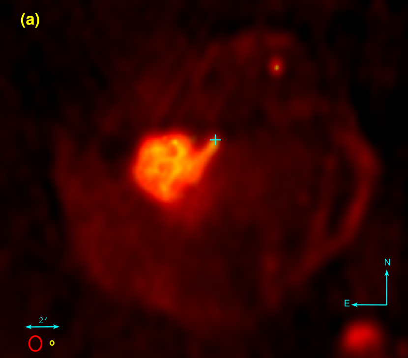
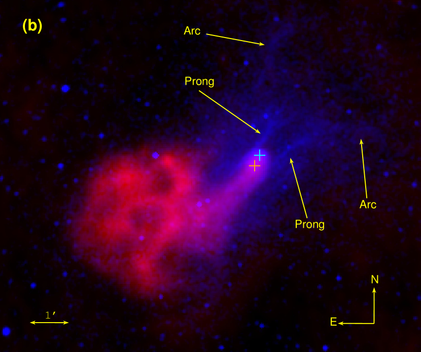
Figure 1.— (a) Composite radio image of SNR G327.1$-$1.1. The MOST 36 cm intensity map (Whiteoak & Green, 1996) is shown in red, illustrating the SNR shell and the PWN. The ATCA 6 cm map is shown in yellow to highlight the detailed structures in the PWN. The radio beams at 36 and 6 cm are shown in the lower left corner as red and yellow ellipses, respectively. The cyan cross marks the position of the X-ray point source reported by Temim et al. (2009), which is believed to be an associated neutron star. Note that the ATCA observations at 6 cm are only sensitive to a scale smaller than $\sim 7^{\prime}$, and therefore are not expected to be sensitive to the SNR shell. (b) Comparison between the radio and X-ray emission of the Snail. The ATCA 6 cm radio image is shown in red and the Chandra ACIS image in $0.5$–$7\,{\rm keV}$ (Temim et al., 2015) is shown in blue. The latter is smoothed to a resolution of $4^{\prime\prime}$. The X-ray point source is marked by the cyan cross and the radio peak is marked by the orange cross. Note that the sizes of the crosses do not represent the respective astrometric uncertainties.

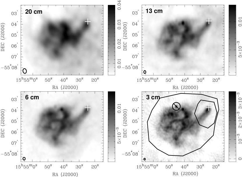
Figure 2.— Radio intensity maps of the Snail at 20, 13, 6, and 3 cm. The restoring beams are shown in the lower left corner of each maps. The grayscales are linear and the scale bars have units of ${\rm Jy\,beam}^{-1}$. The crosses mark the position of the X-ray point source. The regions adopted for flux density measurements are also shown in the 3 cm map. The large polygon indicates the extraction region for flux density measurement of the entire PWN, and the smaller one is for the head only. The body region is that of the entire PWN excluding the head. The crossed out circle centered on the eastern point source is an exclusion region.

For polarimetry, we formed a new set of low-resolution 3 cm images matching that at 6 cm in order to make a direct comparison between the two bands and generate a rotation measure (RM) map (see Section 3.4). A Gaussian taper has been applied to the visibility data by setting the parameter of FWHM $=15$, $13$ in the task INVERT. We then followed the same imaging and cleaning procedures as outlined above, except we convolved the output model of the task PMOSMEM with a Gaussian beam of identical size as the 6 cm beam (${\rm FWHM}=15^{\prime\prime}\times 13^{\prime\prime}$) in the task RESTOR. We obtained polarized intensity and polarization position angle (PA) maps from the Stokes Q and U maps at the two bands. The Ricean bias was corrected for when the polarized intensity was computed (Wardle & Kronberg, 1974). We blanked out areas where either the polarized intensity has S/N $<$ 5 or the total intensity has S/N $<$ 12. Note that polarization was not measured at 20 cm and the 13 cm data are not useful, since the Stokes Q and U maps are corrupted by severe polarization leakage from a nearby bright H ii region G327.3$-$0.6. This is due to a flaw in the feedhorn design of the old ATCA receiver.

For the H i data, we used the task UVLIN to separate line emission from continuum emission within the 20 cm data. We then smoothed the line spectrum to a resolution of $3.3\,{\rm km\,s^{-1}}$ in velocity. To filter out large-scale structures, only data with u-v distances shorter than $1\,{\rm k}\lambda$ were selected to form the line images. We found that the source is too weak to determine any H i absorption.

3. RESULTS

3.1. PWN Morphology

A composite radio image of SNR G327.1$-$1.1 at 36 cm (MOST; Whiteoak & Green, 1996) and 6 cm (ATCA) is shown in Figure 1a, featuring both the SNR shell and the PWN. Radio intensity maps of the PWN at 20, 13, 6, and 3 cm (all from ATCA) are shown in Figure 2. The nebula exhibits similar morphology over the observed wavelengths. It has a main circular structure with a diameter of $\sim 4^{\prime}$ and a finger-like structure of length $\sim 1\farcm 5$ protruding toward the northwest. Together with the two X-ray prongs ahead of the radio finger, the whole PWN resembles a snail. We thus refer to the entire PWN as “the Snail”: the circular structure is the “body” and the protrusion is the

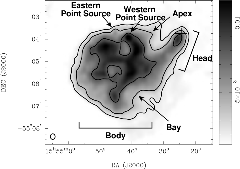
Figure 3.— Structure of the Snail. Both the grayscale and contours are from the 6 cm intensity map, with contour levels set at $2.2$, $4$, and $8\,{\rm mJy\,beam^{-1}}$. The cross marks the position of the X-ray point source. The restoring beam at 6 cm is shown in the lower left corner. The eastern point source can be seen more clearly in the 3 cm image in Figure 2.

“head.” A more detailed look at the body revealed two features — “the bay” to the southwest and “the apex” to the northwest (see Figure 3). The bay is an indented area to the body, while the apex is a sharp corner at the body’s boundary. Faint emission is detected outside of the bay at 20 and 6 cm (about $13.8\,{\rm mJy\,beam^{-1}}$ and $2.5\,{\rm mJy\,beam^{-1}}$, respectively), and was also found in the MOST image (Sun et al., 1999). The emission is not obvious in the 13 and 3 cm images. This could be attributed to the contamination of the 13 cm image by the SNR, while at 3 cm it could be too faint to be detected, or could have been resolved out because of insufficient u-v coverage (see Section 3.2). On a larger scale, hints of an SNR shell of diameter $\sim 17^{\prime}$ are seen in the 20 and 13 cm images (not shown in the field of view of Figure 2). Since the shortest baseline of the 6 and 3 cm observations is 31 m, which translates to angular scales of about $7^{\prime}$ and $4^{\prime}$, respectively, we do not expect these observations to be sensitive to the SNR shell.

The 13, 6, and 3 cm images clearly reveal small-scale structure within the body. We discovered filaments running through the PWN with an unresolved width by our observations. These filaments seem to form loop-like structures that are typically $\sim 1^{\prime}$ diameter. There are two point sources near the northern edge of the body. The eastern one is located at ($15^{\rm h}54^{\rm m}45^{\rm s}$, $-55^{\circ}03^{\prime}39^{\prime\prime}$; J2000.0) and the western one is at ($15^{\rm h}54^{\rm m}41^{\rm s}$, $-55^{\circ}03^{\prime}55^{\prime\prime}$; J2000.0). These are marked in Figure 3. Both point sources are unresolved in the 6 km baseline images, and therefore are less than $1^{\prime\prime}$ in extent.

The head has an extent of about $1\farcm 5$ long and $0\farcm 4$ wide, and shows uniform surface brightness ($\sim 7\,{\rm mJy\,beam^{-1}}$ at 6 cm, and $\sim 2\,{\rm mJy\,beam^{-1}}$ at 3 cm), except near the tip ($15^{\rm h}54^{\rm m}25.4^{\rm s}$, $-55^{\circ}04^{\prime}01.3^{\prime\prime}$; J2000.0) where it shows a peak with $\sim 9\,{\rm mJy\,beam^{-1}}$ at 6 cm and $\sim 3\,{\rm mJy\,beam^{-1}}$ at 3 cm. The radio peak is extended, with a size of $\sim 34^{\prime\prime}\times 18^{\prime\prime}$ elongated along the head, and is offset from the X-ray point source by $\sim 18^{\prime\prime}$ to the southeast. No radio counterparts of the X-ray prongs and arc outside of the head are detected. Careful examination of the 6 km baseline images shows no counterparts of the X-ray point source with a $3\sigma$ upper limit of $1.1\,{\rm mJy}$ at 6 cm.

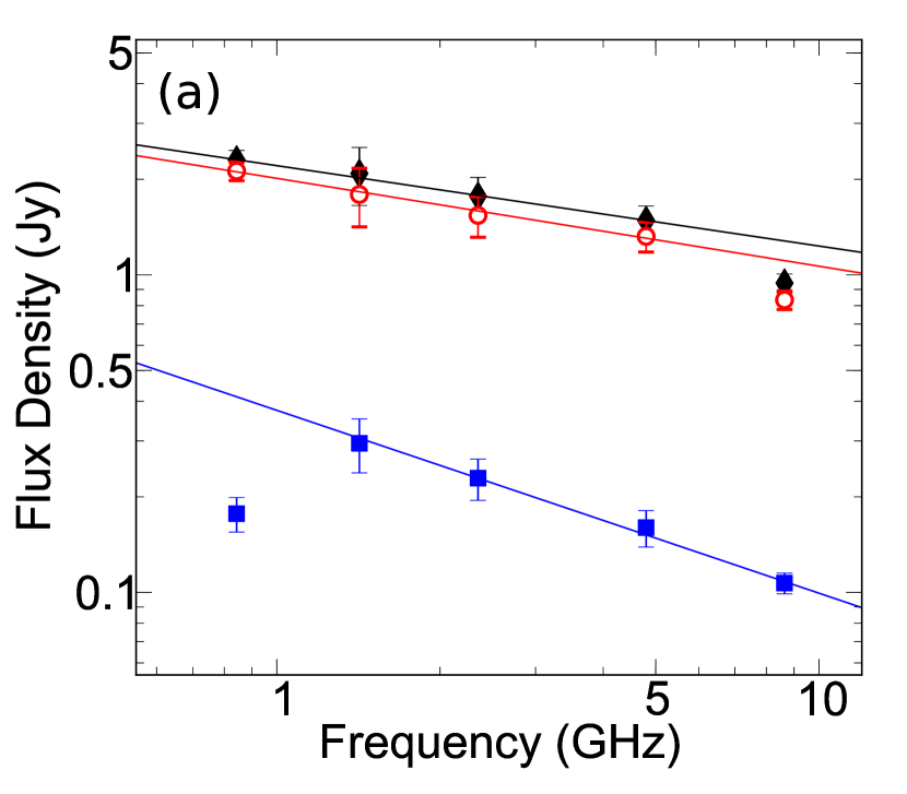
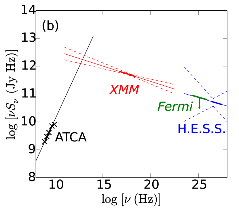
Figure 4.— (a) Radio spectra of the Snail. Flux densities of the entire PWN, the body, and the head are marked by black closed diamonds, red open circles, and blue closed squares, respectively. The best fits to the three spectra give spectral indices of $\alpha=-0.3\pm 0.1$, $-0.3\pm 0.1$, and $-0.6\pm 0.1$, respectively (with $S_{\nu}\propto\nu^{\alpha}$). (b) Spectral energy distribution of the Snail from the radio to TeV band (Temim et al., 2009; Acero et al., 2012, 2013). The best-fit spectra within the respective observed bands are shown as thick solid lines and the extrapolations are shown as thin solid lines. The uncertainties of the fitted spectra are shown as dashed lines.

3.2. Radio Spectrum

To measure the PWN flux density, we employed a source region enclosing both the body and the head as shown in Figure 2. The eastern point source is believed to be a background source while the western point source might be a compact structure within the PWN (see Section 4.1.5). Therefore, we defined a circular exclusion region of $43^{\prime\prime}$ diameter centered at the former. We tried different background regions within the SNR shell, and the difference gives us a handle on the systematic uncertainty. The results are shown in Table 2. The flux densities of the PWN are $2.3\pm 0.2\,{\rm Jy}$, $2.1\pm 0.4\,{\rm Jy}$, $1.8\pm 0.3\,{\rm Jy}$, $1.5\pm 0.2\,{\rm Jy}$, and $0.94\pm 0.06\,{\rm Jy}$ at 36, 20, 13, 6, and 3 cm, respectively. The uncertainties are dominated by the systematic uncertainties associated with background subtraction, as the statistical uncertainties are relatively small (a few mJy). We note that the value we find at 36 cm (2.3 Jy) is slightly larger than that (2.0 Jy) reported by Whiteoak & Green (1996). This could be attributed to our different choice of regions.

The radio spectrum is shown in Figure 4. Fitting the flux densities at 36, 20, 13, and 6 cm with a power law ($S_{\nu}\propto\nu^{\alpha}$) gives a spectral index of $\alpha=-0.3\pm 0.1$, and extrapolation to 3 cm suggests a flux density of $1.3\,{\rm Jy}$, which is almost $40\%$ higher than the observed value of $0.94\,{\rm Jy}$. If we directly join the 6 and 3 cm data points, then we obtain $\alpha=-0.8\pm 0.2$ between the two bands. The shortest u-v spacing at 3 cm is about $0.8\,{\rm k}\lambda$, corresponding to an angular scale of $4\farcm 3$. This sets a rough upper limit on the size of structures that our observations are sensitive to. In order to see if the missing flux problem is significant, we formed a 6 cm radio image only with u-v distance larger than $0.8\,{\rm k}\lambda$, using identical procedure as described in Section 2. This results in about $20\%$ loss in flux density of the PWN, suggesting that the 3 cm observations may not be sensitive to the larger-scale emission of the PWN.

We also determined the flux densities of the body and the head of the Snail separately, with the results also listed in Table 2. The flux densities and fitted spectra are shown in Figure 4. For the body, the flux densities are $2.1\pm 0.1\,{\rm Jy}$, $1.8\pm 0.4\,{\rm Jy}$, $1.5\pm 0.2\,{\rm Jy}$, $1.3\pm 0.1\,{\rm Jy}$, and $0.83\pm 0.06\,{\rm Jy}$ at 36, 20, 13, 6, and 3 cm, respectively, and fitting the flux densities between 36 and 6 cm with a power-law spectrum gives a spectral index of $\alpha=-0.3\pm 0.1$. For the head, the flux densities are $0.18\pm 0.02\,{\rm Jy}$, $0.30\pm 0.06\,{\rm Jy}$, $0.23\pm 0.03\,{\rm Jy}$, $0.16\pm 0.02\,{\rm Jy}$, and $0.11\pm 0.01\,{\rm Jy}$ at 36, 20, 13, 6, and 3 cm, respectively. The spectrum of the head appears to be peculiar, as the observed flux density is lower at 36 cm than that at 20 cm. We believe that the flux density measurement of the head could be affected by faint sidelobes from G327.3$-$0.6 at 36 cm. We fitted the flux densities of the head between 20 and 3 cm, as the size of the head is only about $1\farcm 5$ long and $0\farcm 4$ wide, and should be well sampled by our 3 cm observations. The resulting power-law spectrum has a spectral index of $\alpha=-0.6\pm 0.1$.

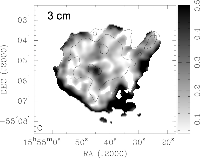
Figure 5.— Fractional polarization of the Snail at 6 and 3 cm. The contours are from the total intensity map of $4$ and $8\,{\rm mJy\,beam}^{-1}$ at 6 cm, and $1.5$ and $4.5\,{\rm mJy\,beam}^{-1}$ at 3 cm. FWHM of the beams are shown in the lower left. The crosses mark the position of the X-ray point source. Note that the polarization at the edge is likely overestimated (see Section 3.3).

The flux densities of the eastern point source are found to be $\sim 2.0\,{\rm mJy}$ at 6 cm and $\sim 3.3\,{\rm mJy}$ at 3 cm, while those for the western point source are $\sim 11\,{\rm mJy}$ at 6 cm and $\sim 7.5\,{\rm mJy}$ at 3 cm. These are very rough estimates, as the diffuse emission from the PWN precludes precise measurements. The results suggest an inverted spectrum with $\alpha\sim+0.9$ for the eastern point source and $\alpha\sim-0.7$ for the western point source.

3.3. Polarization

Maps of the polarization fraction of the Snail at 6 and 3 cm are shown in Figure 5. Overall, the PWN is highly linearly polarized. The typical polarization fraction of the body is about $15\%$ and $20\%$ at 6 and 3 cm, respectively, while that along the head is correspondingly about $20\%$ and $30\%$. At a smaller scale, we found a highly polarized core inside the body as enclosed by an inner contour in Figure 5, with polarization fractions of about $30\%$ and $40\%$ at 6 and 3 cm, respectively. Near the northern edge of the body, the eastern point source is unpolarized, while the western point source is about $10\%$ polarized at both bands. Note that the actual polarization fraction at 3 cm could be lower due to the missing flux problem as mentioned. Finally, the polarization fraction at the edge of the body may be overestimated because we have used only a single RMS value for the debiasing procedure.

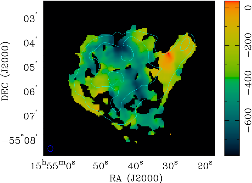
Figure 6.— RM map of the Snail. Contours are from the 6 cm image of the PWN at levels of $4$ and $8\,{\rm mJy\,beam}^{-1}$. The color map represents the RM distribution of the Snail in units of $\rm{rad\,m}^{-2}$. The restoring beam is shown at the lower left corner.

3.4. RM of the Snail

We generated an RM map by comparing between the polarization PA maps at 6 and 3 cm:

$${\rm RM}=\frac{\chi_{6}-\chi_{3}}{\lambda_{6}^{2}-\lambda_{3}^{2}}~{}{\rm,}$$ (1)

where $\chi_{6}$ and $\chi_{3}$ are the observed PAs in the respective bands, and $\lambda_{6}$ and $\lambda_{3}$ are the center wavelengths of the bands. The resulting RM map is shown in Figure 6, and the RM is found to vary smoothly between $-800$ and $0\,{\rm rad\,m^{-2}}$ across the PWN with a typical uncertainty of $25\,{\rm rad\,m^{-2}}$. The average RM value is about $-380\,{\rm rad\,m^{-2}}$.

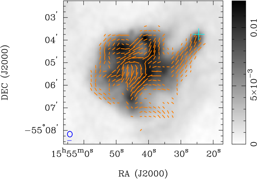
Figure 7.— Intrinsic magnetic field configuration of the Snail. The direction of the vectors shows the orientation of the magnetic field corrected for Faraday rotation, and the length is proportional to the polarized intensity with the scale bar at the lower left representing $1\,{\rm mJy\,beam}^{-1}$. Typical uncertainty in PA is about $3^{\circ}$. The grayscale shows the radio intensity at 6 cm with the scale bar in units of ${\rm Jy\,beam}^{-1}$. FWHM of the beam is shown by the ellipse at the lower left. The cross marks the position of the X-ray point source.

One problem of determining the RM this way is the so-called $n\pi$ ambiguity. This ambiguity arises because an RM of larger magnitude can also be compatible with the observed polarization vectors if it provides an addition of multiples of $\pi$ radian to the relative rotation between the two bands. For example, adding an extra RM of $1160\,{\rm rad\,m}^{-2}$ can rotate the polarization vectors at 6 and 3 cm by $\pi\,{\rm radian}$ relative to each other. In order to eradicate this problem, we picked the first and last channels of the 6 cm data, which are at frequencies of $4848\,{\rm MHz}$ and $4752\,{\rm MHz}$, respectively, and formed PA maps separately using procedures identical to those of the full-band data. By applying the PA maps, we generated an RM map from the two channels. Because the individual pixels of the RM map have large uncertainty, we did not attempt to investigate the spatial distribution of the RM from it. Instead, we averaged the RM across the entire PWN to boost the S/N ratio, and found an average RM for the Snail of $-380\,{\rm rad\,m}^{-2}$ from the two channels, which is identical to the value obtained above. Since we expect the rotation of the PA within the 6 cm band to be small (less than $\pi\,{\rm radian}$, otherwise the bandwidth depolarization would have been significant), this rules out the $n\pi$ ambiguity in our measurements.

3.5. Intrinsic Magnetic Field Orientation

We employed the RM map obtained from Section 3.4 to derotate the polarization vectors at 6 and 3 cm in order to infer the intrinsic magnetic field orientation of the PWN. Since the RM was derived from the PAs at 6 and 3 cm only, the derotated vectors at the two bands have identical orientation. The derotated vectors have a typical uncertainty of about $3^{\circ}$, contributed by both the error in PA and in RM. Figure 7 shows the projected intrinsic magnetic field orientation of the Snail. Overall, the field is highly ordered. The magnetic field at the head aligns with the PWN elongation, while for the body it is tangential to the boundary, except at the apex where it becomes radial. The field configuration of the interior of the body is complex with the magnetic field generally following the filamentary loops.

4. DISCUSSION

4.1. PWN Structure and Magnetic Field Geometry

4.1.1 Overall PWN

The Snail is believed to have first encountered the reverse shock about $10\,{\rm kyr}$ ago, as suggested by HD simulations (Temim et al., 2015). This could have resulted in a turbulent environment in the PWN and given rise to a tangled magnetic field geometry. The strong polarization signal we found from the Snail indicates the presence of a highly ordered magnetic field. This could reflect a turbulence scale larger than the beam size of our observations. In this case, the beam depolarization will be insignificant and the observed magnetic field geometry will appear ordered at small scales. For further investigation, MHD efforts are required to fully understand the highly ordered magnetic field found in the Snail.

4.1.2 The Head

The magnetic field in the head of the Snail shows good alignment with the elongation of the structure (see Figure 7). This is consistent with the evolutionary picture suggested by Temim et al. (2009), assuming that the magnetic field lines are frozen in the newly generated pulsar wind being pushed to the southeast. Similar magnetic field geometry is also found in some bow-shock PWNe, including the “handle” of the Frying Pan (G315.78$-$0.23; Ng et al., 2012) and the tail of the Mouse (G359.23$-$0.82; Yusef-Zadeh & Gaensler, 2005). However, a distinctly different example is the bow-shock system G319.9$-$0.7, which shows a helical magnetic field which then aligns with the flow further downstream (Ng et al., 2010). The cause of such a peculiar configuration is not well understood, though it may be related to the Mach number of the pulsar with respect to its ambient medium or the relative inclination of the spin axis and the elongation of the PWN (e.g., Ng et al., 2010, 2012). As the head of the Snail is believed to be a non-bow-shock system (i.e. the Mach number of the neutron star $<1$; van der Swaluw et al., 2004; Temim et al., 2009, 2015), it serves as an example showing that magnetic field can align with subsonic comet-like PWNe.

We also compare the field geometry around the presumed pulsar with those of a few evolved PWNe, including Vela X (Bock et al., 1998; Dodson et al., 2003), the Boomerang (G106.6$+$2.9; Kothes et al., 2006), and DA 495 (G65.7$+$1.2; Kothes et al., 2008). These PWNe could also have been crushed by the reverse shocks. The Boomerang and DA 495 have diameters of about $1\,{\rm pc}$ and $4\,{\rm pc}$, respectively. They are considerably smaller than the Snail, which has a length of the head spanning $4\,{\rm pc}$ and the diameter of the body stretching $10\,{\rm pc}$. The radio polarimetric observation of Vela X (Dodson et al., 2003) only covered the immediate vicinity ($\sim 0.4\,{\rm pc}$) around the Vela pulsar. In the Boomerang and Vela X, toroidal magnetic fields can be observed, while in DA 495 it was suggested to present a toroidal component superimposed on the apparently dipolar field structure. The magnetic field structures in these three PWNe could be driven by the pulsar itself (Dodson et al., 2003; Kothes et al., 2006, 2008), while in the head of the Snail the magnetic field lines parallel to the nebulae elongation can be shaped by the passage of the reverse shock. Note that the physical scale for which we have resolution of in the Snail is very different from that of the three presented above. Future high-resolution studies may potentially probe the pulsar-driven field near the presumed pulsar of the Snail.

4.1.3 Filaments in the Body

The high spatial resolution ATCA images in Figure 2 revealed the filamentary structure inside the PWN. The filamentary loops generally align with the magnetic field (see Figure 7), suggesting that they could be magnetic loops similar to those observed in young PWNe 3C 58 (Slane et al., 2004) and G54.1$+$0.3 (Lang et al., 2010). In the Snail, the filamentary loops have a typical diameter of $\sim 1^{\prime}$, which corresponds to $2.6\,{\rm pc}$ at a distance of $9\,{\rm kpc}$. The scale is a few times larger than those in 3C 58 and G54.1$+$0.3, which were estimated to have diameters of about $0.3$–$0.5\,{\rm pc}$ and $0.5$–$0.9\,{\rm pc}$, respectively (Slane et al., 2004; Lang et al., 2010). It was suggested that kink instabilities can be the origin of magnetic loops in PWNe — the toroidal field near the termination shock could be torn away and eventually become a magnetic loop as observed (Slane et al., 2004). However, it is unclear if the interaction of the SNR reverse shock could destroy these structures. In this case, the loops would be formed through another mechanism.

4.1.4 The Apex and the Bay

We identified two structures of the Snail near the edge of the body referred to as the apex and the bay. The former could be a protrusion from the body, but it is difficult to confirm because its proximity to the head complicates the interpretation of the morphology. The magnetic field vectors at the apex show a radial instead of tangential orientation as seen in other parts of the PWN boundary. Similar protrusions and chimney-like structures are seen in the Crab Nebula (Bietenholz & Kronberg, 1990) and in Kes 75 (Ng et al., 2008). The apex could be formed by the leakage of PWN materials into the surrounding shocked SN ejecta, similar to the chimney of the Crab Nebula. However, one difference between the Crab Nebula and the body of the Snail is that the boundary magnetic field of the Crab Nebula is primarily radial (Bietenholz & Kronberg, 1990), and so the physical processes appear to be different.

The nature of the faint emission outside of the bay, which is outlined by the outermost contour in Figure 3, could be important for understanding the evolution scenario of G327.1$-$1.1. It has been suggested as part of the PWN (Sun et al., 1999), implying that the true boundary of the PWN should lie outside the bay, such that the head would be pointing closer to the center of the body as suggested by simulations (Temim et al., 2015), instead of being tangential to its edge.

4.1.5 Eastern and Western Point Sources

As pointed out in Section 3.1, our radio maps revealed two point sources in the northern edge of the PWN. We found that the eastern one is unpolarized (Figure 5) and has an inverted spectrum of $\alpha\sim+0.9$, which differs significantly from the typical value of $-0.3\lesssim\alpha\lesssim 0$ for PWNe. These points suggest that it is likely an unrelated background source.

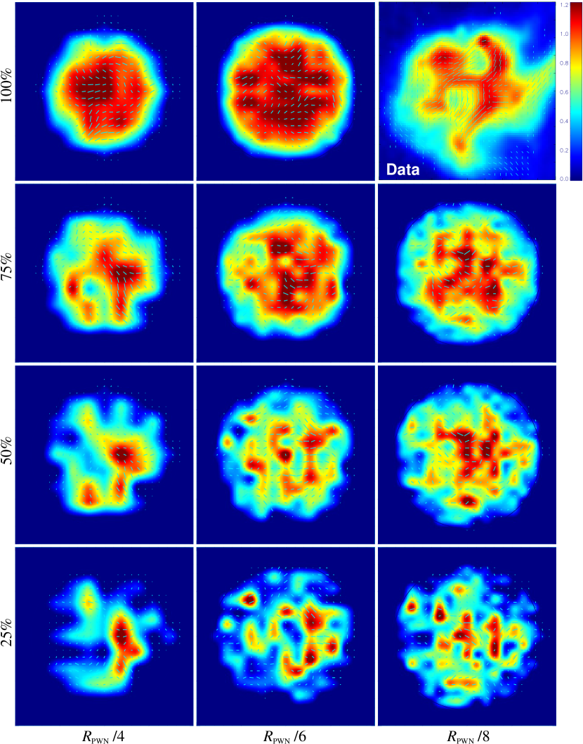
Figure 8.— Simulated intensity maps of a spherical PWN overlaid by the polarization vectors compared with the data. The orientations of the vectors show the nebular $B$-field directions and the lengths represent the polarized intensity. Each model is comprised of patches of a certain size as indicated at the bottom, with the magnetic field orientation randomly chosen for each of the patches. The pulsar wind filling factor is also indicated to the left. The observations of the Snail at 6 cm are shown in the upper right panel with the same color scale.

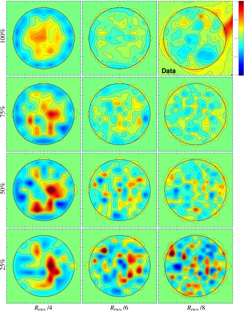
Figure 9.— Intensity maps in Figure 8 subtracted by the mean emissivity to show the fluctuation due to turbulence. The filling factors and patch sizes are indicated at the left and bottom, respectively (see text for details). The subtracted intensity map of the Snail is shown in the upper right panel.

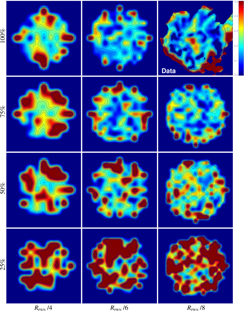
Figure 10.— Simulated polarization maps compared with the data. The filling factors and patch sizes are indicated at the left and bottom, respectively (see text for details). The polarization map of the Snail at 6 cm is shown in the upper right panel. We note that the large polarization fraction near the edge of the PWN is mostly due to noise, as the radio emission is weak.

On the other hand, the western source has a spectral index of $\alpha\sim-0.7$ and is about $10\%$ polarized at 6 and 3 cm. The polarized emission allows us to determine the RM of the source and its value is consistent with that of the surrounding PWN (see Figure 6), suggesting a similar distance. It also spatially coincides with the filaments in the PWN. Therefore, we argue that it is associated with the Snail, possibly an unresolved compact knot as part of the filaments.

4.2. Simple Modeling of Turbulence in the Snail

As mentioned earlier, the highly ordered magnetic field found in the Snail could imply a large characteristic scale of the turbulence. To get a handle on the scale in this case, we consider a toy model of the body of the Snail (i.e. excluding the head) as a non-evolving spherical nebula. This assumption is based on the fact that we do not expect significant multipolar anisotropy in the pressure exerted by the reverse shock, except for the dipolar component, which will displace the PWN instead of deforming it. The volume of the nebula is divided into patches of uniform size that represent the characteristic turbulence scale in the PWN. The turbulent magnetic field is implemented in our model by assigning a magnetic field with random orientation but uniform strength to each of the patches. We argue that this assumption is justified, as the magnetic field inferred from simulations (Temim et al., 2015) is close to the equipartition value we derived in Section 4.4 below, and therefore the fluctuations in the magnetic field strength should be small. Otherwise, the fluctuation will rapidly fade away over a timescale of the order of the sound crossing time (which is much shorter than the age of the system). The electron density is also assumed to be uniform for the same reason, and we assume a power-law distribution with the index given by the measured radio spectrum. We further allow for the possibility that a patch is filled with cold SNR material instead of non-thermal pulsar wind particles. This mixing of SN ejecta in the Snail was suggested based on X-ray observations (Temim et al., 2015) and can also be seen in other reverse shock crushed PWNe such as Vela X (LaMassa et al., 2008). The probability that a patch is filled by synchrotron-emitting pulsar wind particles is simply the filling factor in our model. If there is no significant mixing of materials in the PWN, then the modeling results with a filling factor of $100\%$ should fit the observations best, while a lower filling factor would suggest substantial mixing.

We integrated the synchrotron emission along different lines of sight through the volume of the nebula in all of the Stokes parameters to compute the radio maps for comparisons with our observations. For this, we convolved the simulation results with the radio beam. Note that the randomness introduced by the filling factor and the magnetic field orientations make it possible to exactly reproduce the observations if we run the model for a considerable number of times (albeit that will be meaningless), and therefore it is more sensible to only produce one set of maps per combination of parameters, and then inspect by eye the scales of the structures, the number of features in the PWN, and the contrast in radio intensity instead of looking for a perfect match. This allows us to place a rough constraint on the filling factor and the characteristic turbulence scale of the Snail. The simulated intensity and fluctuation maps are shown in Figures 8 and 9. A filling factor of 50–75% and a patch size of 1/8–1/6 of the PWN radius ($R_{\rm PWN}$) appear to give the best match between the simulations and the data, such that they have comparable numbers of small-scale features and contrast in the intensity maps. In Figure 10 we show the simulated polarization maps. A large filling factor or small patch size generally give a lower polarization fraction. This is because, as there are more patches with different $B$-field orientation along a line of sight, depolarization becomes more severe. We find that the same range of filling factor and patch size as above provide the best fit to the observation. If this simple model is true, then the simulation results suggest that mixing in this PWN is significant and the turbulence scale is about $R_{\rm PWN}/8$ – $R_{\rm PWN}/6$. The former conclusion is in line with the speculation of Temim et al. (2015), and should be taken into account for further theoretical work with the Snail. Finally, we note that the randomly oriented magnetic field in this simple model does not satisfy the solenoid condition (i.e., $\nabla\cdot B=0$). Therefore, it fails to reproduce the magnetic loops in the PWN interior and the tangential field structure at the boundary as observed. Instead, it is more useful to compare the coherence scales of the models with the observations.

4.3. Radio Spectrum of the Snail

We determined a spectral index of $\alpha=-0.3\pm 0.1$ for the Snail between 36 and 6 cm. Such a flat spectrum is typical for PWNe. The flux density at 3 cm is not well determined as the observations are only sensitive to smaller structures in the PWN but not the whole nebula. The head of the Snail has a steeper spectral index of $\alpha=-0.6\pm 0.1$. This is unexpected, as X-ray observations suggest that the particles are injected from the head (e.g. Sun et al., 1999; Temim et al., 2009, 2015), and therefore the materials in the head should be younger than those of the body. This means that the spectral difference probably cannot be explained by synchrotron cooling. We also note that this spectral index is considerably steeper than the generally expected value for PWNe ($-0.3\leq\alpha\leq 0$), which is rather unusual and requires further theoretical modeling to explain.

4.4. Minimum-energy Magnetic Field Strength in the PWN

We computed the minimum-energy magnetic field strength by imposing the conventional assumption, i.e. that the total energy $U_{\rm total}$ is distributed between magnetic energy $U_{B}$ and particle energy $U_{p}$ in a way that $U_{\rm total}$ is minimized. From synchrotron theory (Pacholczyk, 1970), we have

$$U_{\rm total}=U_{B}+U_{p}=\frac{B^{2}}{8\pi}\Phi V+c_{12}(1+\eta)L_{\rm syn}B^{-3/2}{\rm,}$$ (2)

where $\Phi$ is the volume filling factor of the magnetic field, $V$ is the volume of the emission region, $c_{12}$ is a constant weakly depending on the spectral index and frequency range considered, $\eta$ is the energy ratio of ions to electrons, and $L_{\rm syn}$ is the synchrotron luminosity of the PWN. Minimizing $U_{\rm total}$ gives a minimum-energy field,

$$B_{\rm m}=\left[6\pi c_{12}(1+\eta)L_{\rm syn}\Phi^{-1}V^{-1}\right]^{2/7}{\rm,}$$ (3)

which is also referred to as the “equipartition field” in some literature. We integrated the simple power-law radio spectrum for the entire PWN (as in the fit of Figure 4) between $10^{7}$ and $10^{13}\,{\rm Hz}$ (e.g. Ng et al., 2010, 2012), and found $L_{\rm syn}=2.9\times 10^{35}d_{9}^{2}\,{\rm erg\,s}^{-1}$, where $d_{9}$ is the distance to the Snail in units of $9\,{\rm kpc}$. To estimate the volume $V$, we modeled the body as a sphere of diameter $4^{\prime}$ and the head as a cylinder with a diameter of $0\farcm 4$ and a length of $1\farcm 5$. The volume of the PWN is then $V=1.8\times 10^{58}d_{9}^{3}\,{\rm cm}^{3}$. Substituting these parameters into Equation 3 gives

$$B_{\rm m}=36(1+\eta)^{2/7}\Phi^{-2/7}d_{9}^{-2/7}\,{\rm\mu G.}$$ (4)

Assuming $\eta=0$, $\Phi=1$, and $d_{9}=1$, we find a minimum-energy field of $36\,{\rm\mu G}$ in the Snail, which is of the same order of magnitude as that estimated by modeling the broadband emission of the PWN ($11\,\mu{\rm G}$; Temim et al., 2015). Note that the computed minimum-energy field strength can depend on the frequency range chosen. For instance, if we only integrate up to $10^{11}\,{\rm Hz}$ instead of $10^{13}\,{\rm Hz}$, then we obtain a slightly lower value of $26\,\mu{\rm G}$, and it is much less sensitive to the lower frequency limit. It is also worth noting that the energy in the pulsar wind is believed to be particle-dominated upon injection, and hence the minimum-energy condition is not guaranteed to hold.

We also computed the minimum-energy field strength of the body and the head separately, using identical procedures as above. For the body, we have $L_{\rm syn,body}=2.1\times 10^{35}\,{\rm erg\,s}^{-1}$ and $V_{\rm body}=1.8\times 10^{58}\,{\rm cm}^{3}$, which gives $B_{\rm m,body}=34\,\mu{\rm G}$. For the head, we have $L_{\rm syn,head}=4.1\times 10^{33}\,{\rm erg\,s}^{-1}$ and $V_{\rm head}=9.9\times 10^{55}\,{\rm cm}^{3}$, which gives $B_{\rm m,head}=69\,\mu{\rm G}$. The higher minimum-energy field strength in the head as compared to that in the body could suggest that the reverse shock has compressed the former but not yet the latter.

4.5. Multiwavelength Comparison

Figure 1b shows that the radio peak of the head is offset from the X-ray point source by $\sim 18^{\prime\prime}$ (corresponding to $0.8\,{\rm pc}$ at a distance of $9\,{\rm kpc}$), which is larger than the astrometric uncertainty of $\sim 1^{\prime\prime}$ of Chandra and the radio beam size (${\rm FWHM}\sim 15^{\prime\prime}$). A similar offset is found in other systems, including G319.9$-$0.7 (Ng et al., 2010) and the Lighthouse Nebula (Pavan et al., 2014) powered by PSR J1101$-$6101 (Halpern et al., 2014), in which the radio and X-ray peaks are displaced by $4\,{\rm pc}$ and $0.7\,{\rm pc}$, respectively. On the other hand, there is no detectable radio emission at the location of the X-ray prongs and arc of the Snail. This is analogous to the X-ray jet-like structures seen in the Guitar Nebula (Hui & Becker, 2007) and the Lighthouse Nebula (Pavan et al., 2014). This could be the result of the diffusion of high-energy particles, but the density is too low for the radio emission to be detected. We also note that the prong structures are aligned with the edge of the radio head.

The broadband synchrotron spectra of PWNe often steepen at high frequency due to synchrotron cooling. For a single population of particles injected into the system, the spectral break frequency $\nu_{b}$ and magnetic field strength $B$ could be used to estimate the PWN age $\tau$ by (Gaensler & Slane, 2006)

$$\tau=\left(\frac{\nu_{b}}{10^{21}\,{\rm Hz}}\right)^{-1/2}\left(\frac{B}{10^{-6}\,{\rm G}}\right)^{-3/2}\,{\rm kyr.}$$ (5)

Using the $\nu_{\rm b}=10^{13}\,{\rm Hz}$ obtained through extrapolation of radio and X-ray spectra (Figure 4b) and the minimum-energy field strength obtained above ($B_{\rm m}=36\,\mu{\rm G}$) gives $\tau=46\,{\rm kyr}$ for the Snail. If we instead use the magnetic field strength estimate from modeling ($11\,\mu{\rm G}$; Temim et al., 2015), then we acquire an even larger $\tau=270\,{\rm kyr}$. These values differ significantly from the age estimates of $11$–$29\,{\rm kyr}$ from previous studies (Sun et al., 1999; Bocchino & Bandiera, 2003; Temim et al., 2009, 2015). We argue that the simple estimate from the spectral break may not reflect the true age of the system. The change in spectral index by a simple extrapolation of the radio and X-ray spectra is $\Delta\alpha\approx 0.9$. This suggests that the actual spectral energy distribution (SED) of the system can be much more complicated than expected, as the result of a broken power-law injection spectrum and enhanced synchrotron burnoff induced by the reverse shock interaction (see Temim et al., 2015). This can be verified by future observations between the radio and X-ray bands.

Figure 4b shows the broadband SED of the Snail from radio to $\gamma$-rays, with the $\gamma$-ray data from Fermi and H.E.S.S. (Acero et al., 2012, 2013). While the TeV $\gamma$-ray spectrum from H.E.S.S. appears to align with the X-ray spectrum, this is probably just coincidence (see Temim et al., 2015).

5. CONCLUSION

In this paper, we presented radio observations of the Snail PWN in SNR G327.1$-$1.1 using ATCA and compared the results with the previous MOST study (Whiteoak & Green, 1996). The PWN shows the same morphology in all the five bands between 36 and 3 cm, consisting of a main circular body believed to be the “relic” PWN and a protruding head. The 6 and 3 cm polarization maps reveal a highly ordered magnetic field structure, in contrast with the turbulent interior with a tangled magnetic field structure expected for a reverse shock crushed PWN. This may suggest that the characteristic turbulence scale is larger than the radio beam size. To explore this scenario, we developed a toy model to simulate the emission from a turbulent PWN and found that a characteristic turbulence scale of $\sim R_{\rm PWN}/8$ – $R_{\rm PWN}/6$ with a filling factor of $50$–$75\%$ can most closely match the observations.

We showed that the magnetic field at the head of the Snail aligns with the nebular elongation. This serves as a good example of subsonic cometary PWN systems with magnetic field parallel to the tail. In addition, we discovered filamentary structures in the body which could be magnetic loops. It is, however, unclear whether they are formed by kink instabilities as suggested for 3C 58 and G54.1$+$0.3, or by turbulence during the reverse shock interaction. We also determined a spectral index of $\alpha=-0.3\pm 0.1$ for the overall PWN in the observed radio bands, which gives a minimum-energy magnetic field strength of $B_{\rm m}\approx 36\,\mu{\rm G}$. The radio spectrum of the head appears to be steeper than that of the body, which is difficult to explain through synchrotron cooling.

References

- Acero et al. (2013) Acero, F., Ackermann, M., Ajello, M., et al. 2013, ApJ, 773, 77
- Acero et al. (2015) Acero, F., Ackermann, M., Ajello, M., et al. 2015, arXiv:1511.06778
- Acero et al. (2012) Acero, F., Djannati-Ataï, A., Förster, A., et al. 2012, arXiv:1201.0481
- Bietenholz & Kronberg (1990) Bietenholz, M. F., & Kronberg, P. P. 1990, ApJL, 357, L13
- Blondin et al. (2001) Blondin, J. M., Chevalier, R. A., & Frierson, D. M. 2001, ApJ, 563, 806
- Bocchino & Bandiera (2003) Bocchino, F., & Bandiera, R. 2003, A&A, 398, 195
- Bock et al. (1998) Bock, D. C.-J., Turtle, A. J., & Green, A. J. 1998, ApJ, 116, 1886
- Briggs (1995) Briggs, D. S. 1995, BAAS, 27, 1444
- Clark et al. (1973) Clark, D. H., Caswell, J. L., & Green, A. J. 1973, Natur, 246, 28
- Clark et al. (1975) Clark, D. H., Caswell, J. L., & Green, A. J. 1975, AuJPA, 37, 1
- Dodson et al. (2003) Dodson, R., Lewis, D., McConnell, D., & Deshpande, A. A. 2003, MNRAS, 343, 116
- Gaensler & Slane (2006) Gaensler, B. M., & Slane, P. O. 2006, ARA&A, 44, 17
- Gelfand et al. (2009) Gelfand, J. D., Slane, P. O., & Zhang, W. 2009, ApJ, 703, 2051
- Gull & Daniell (1978) Gull, S. F., & Daniell, G. J. 1978, Natur, 272, 686
- Halpern et al. (2014) Halpern, J. P., Tomsick, J. A., Gotthelf, E. V., et al. 2014, ApJL, 795, L27
- Hui & Becker (2007) Hui, C. Y., & Becker, W. 2007, A&A, 467, 1209
- Kothes et al. (2008) Kothes, R., Landecker, T. L., Reich, W., Safi-Harb, S., & Arzoumanian, Z. 2008, ApJ, 687, 516
- Kothes et al. (2006) Kothes, R., Reich, W., & Uyanıker, B. 2006, ApJ, 638, 225
- LaMassa et al. (2008) LaMassa, S. M., Slane, P. O., & de Jager, O. C. 2008, ApJL, 689, L121
- Lamb & Markert (1981) Lamb, R. C., & Markert, T. H. 1981, ApJ, 244, 94
- Lang et al. (2010) Lang, C. C., Wang, Q. D., Lu, F., & Clubb, K. I. 2010, ApJ, 709, 1125
- Ng et al. (2012) Ng, C.-Y., Bucciantini, N., Gaensler, B. M., et al. 2012, ApJ, 746, 105
- Ng et al. (2010) Ng, C.-Y., Gaensler, B. M., Chatterjee, S., & Johnston, S. 2010, ApJ, 712, 596
- Ng et al. (2008) Ng, C.-Y., Slane, P. O., Gaensler, B. M., & Hughes, J. P. 2008, ApJ, 686, 508
- Pacholczyk (1970) Pacholczyk, A. G. 1970, Radio Astrophysics: Nonthermal Processes in Galactic and Extragalactic Sources (San Francisco, CA: Freeman)
- Pavan et al. (2014) Pavan, L., Bordas, P., Pühlhofer, G., et al. 2014, A&A, 562, A122
- Sault et al. (1999) Sault, R. J., Bock, D. C.-J., & Duncan, A. R. 1999, A&AS, 139, 387
- Sault et al. (1995) Sault, R. J., Teuben, P. J., & Wright, M. C. H. 1995, in ASP Conf. Ser. 77, Astronomical Data Analysis Software and Systems IV, ed. R. A. Shaw, H. E. Payne, & J. J. E. Hayes (San Francisco, CA: ASP), 433
- Sault & Wieringa (1994) Sault, R. J., & Wieringa, M. H. 1994, A&AS, 108, 585
- Seward et al. (1996) Seward, F. D., Kearns, K. E., & Rhode, K. L. 1996, ApJ, 471, 887
- Slane et al. (2004) Slane, P., Helfand, D. J., van der Swaluw, E., & Murray, S. S. 2004, ApJ, 616, 403
- Sun et al. (1999) Sun, M., Wang, Z.-r., & Chen, Y. 1999, ApJ, 511, 274
- Temim et al. (2009) Temim, T., Slane, P., Gaensler, B. M., Hughes, J. P., & van der Swaluw, E. 2009, ApJ, 691, 895
- Temim et al. (2015) Temim, T., Slane, P., Kolb, C., et al. 2015, ApJ, 808, 100
- van der Swaluw et al. (2001) van der Swaluw, E., Achterberg, A., Gallant, Y. A., & Tóth, G. 2001, A&A, 380, 309
- van der Swaluw et al. (2004) van der Swaluw, E., Downes, T. P., & Keegan, R. 2004, A&A, 420, 937
- Wardle & Kronberg (1974) Wardle, J. F. C., & Kronberg, P. P. 1974, ApJ, 194, 249
- Whiteoak & Green (1996) Whiteoak, J. B. Z., & Green, A. J. 1996, A&AS, 118, 329
- Wilson et al. (2011) Wilson, W. E., Ferris, R. H., Axtens, P., et al. 2011, MNRAS, 416, 832
- Yusef-Zadeh & Gaensler (2005) Yusef-Zadeh, F., & Gaensler, B. M. 2005, AdSpR, 35, 1129