Reaction Time for Trimolecular Reactions in
Compartment-based Reaction-Diffusion Models

Abstract

Trimolecular reaction models are investigated in the compartment-based (lattice-based) framework for stochastic reaction-diffusion modelling. The formulae for the first collision time and the mean reaction time are derived for the case where three molecules are present in the solution.

I Introduction

Trimolecular reactions are important components of biochemical models which include oscillations Schnakenberg:1979:SCR , multistable states Schlogl:1972:CRM and pattern formation Qiao:2006:SDS . Considering their reactant complexes, trimolecular reactions can be subdivided into the following three forms

$$3U \displaystyle\mathop{\longrightarrow} \emptyset,$$ (1)

$$2U+V \displaystyle\mathop{\longrightarrow} \emptyset,$$ (2)

$$U+V+W \displaystyle\mathop{\longrightarrow} \emptyset,$$ (3)

where $U$, $V$ and $W$ are distinct chemical species (reactants) and symbol $\emptyset$ denotes products. In what follows, we will assume that product complexes $\emptyset$ do not include $U$, $V$ and $W$. Let us denote by $u$ the concentration of $U$. Then the conventional reaction-rate equation for trimolecular reaction (1) can be written as

$$\frac{\mbox{d}u}{\mbox{d}t}=-k(t)\,u^{3},$$ (4)

where $k(t)$ denotes (in general, time-dependent) reaction rate constant Oshanin:1995:SAT . Using mass-action kinetics, rate $k(t)$ is assumed to be constant and equation (4) becomes an autonomous ordinary differential equation (ODE) with a cubic nonlinearity on its right-hand side. Cubic nonlinearities significantly enrich the dynamics of ODEs. For example, ODEs describing chemical systems with two chemical species which do not include cubic or higher nonlinearites cannot have any limit cycles Plesa:2015:CRS . On the other hand, it has been reported that, by adding cubic nonlinearities to such systems, one can obtain chemical systems undergoing homoclinic Plesa:2015:CRS and SNIC bifurcations Erban:2009:ASC , i.e. oscillating solutions are present for some parameter regimes.

Motivated by the developments in systems biology Paulsson:2000:SFF ; Elowitz:2002:SGE , there has been an increased interest in recent years in stochastic methods for simulating chemical reaction networks. Such approaches provide detailed information about individual reaction events. Considering well-mixed reactors, this problem is well understood. The method of choice is the Gillespie algorithm Gillespie:1977:ESS or its equivalent formulations Gibson:2000:EES ; Cao:2004:EFS . These methods describe stochastic chemical reaction networks as continous-time discrete-space Markov chains. They are applicable to modelling intracellular reaction networks in relatively small domains which can be considered well-mixed by diffusion. If this assumption is not satisfied, then stochastic simulation algorithms for spatially distributed reaction-diffusion systems have to be applied Erban:2007:PGS ; Erban:2007:RBC . The most common algorithms for spatial stochastic modelling in systems biology can be classified as either Brownian dynamics (molecular-based) Andrews:2004:SSC ; Takahashi:2010:STC or compartment-based (lattice-based) approaches Hattne:2005:SRD ; Engblom:2009:SSR . Molecular-based models describe a trajectory of each molecule involved in a reaction network as a standard Brownian motion. This can be justified as an approximation of interactions (non-reactive collisions) with surrounding molecules (heat bath) on sufficiently long time scales Erban:2014:MDB ; Erban:2015:CAM . It is then often postulated that bimolecular or trimolecular reactions occur (with some probability) if the reactant molecules are sufficiently close Oshanin:1995:SAT ; Erban:2009:SMR ; Agbanusi:2013:CBR ; Flegg:2015:SRK .

Brownian dynamics treatment of bimolecular reactions is based on the theory of diffusion-limited reactions, which postulates that a bimolecular reaction occurs if two reactants are within distance $R$ (reaction radius) from each other. The properties of this model depend on the physical dimension of the reactor. Considering one-dimensional Torney:1983:DRO and two-dimensional problems Torney:1983:DRR , diffusion-limited reactions lead to mean-field models with time-dependent rate constants which converge to zero for large times. This qualitative property is in one spatial dimension shared by trimolecular reactions. It has been shown that the mean-field model (4) can be obtained with time-dependent rate constant $k(t)$ satisfying for large times

$$k(t)\approx C\sqrt{\frac{\log t}{t}},$$ (5)

where $C$ is a constant benAvraham:1993:DTR ; Oshanin:1995:SAT . Considering three-dimensional problems, the reaction radius of a diffusion-limited bimolecular reaction can be related with a (time-independent) reaction rate of the corresponding mean-field model Erban:2009:SMR . Trimolecular reaction (1) can then be incorporated into three-dimensional Brownian dynamics simulations either directly Flegg:2015:SRK or as a pair of bimolecular reactions $U+U\displaystyle\mathop{\longrightarrow}Z$ and $Z+U\displaystyle\mathop{\longrightarrow}\emptyset$, where $Z$ denotes a dimer of $U$ Gillespie:1992:MPI .

Compartment-based models divide the simulation domain into compartments (voxels) and describe the state of the system by numbers of molecules in each compartment. Compartments can be both regular (cubic lattice) or irregular (unstructured meshes) Engblom:2009:SSR . Considering that the simulation domain is divided into cubes of side $h$, the diffusive movement of molecules of $U$ is then modelled as jumps between neighbouring compartments with rate $d_{u}=D_{u}/h^{2}$, where $D_{u}$ is the diffusion constant of the chemical species $U$. In this paper, we will consider compartment-based stochatic reaction-diffusion models of the trimolecular reactions (1)–(3) in a narrow domain $[0,L]\times[0,h]\times[0,h]$ where $L\gg h$. Such domains are useful for modelling filopodia Erban:2014:MSR , but they can also be viewed as a simplification of a real three-dimensional geometry when there is no variation in $y$ and $z$ directions. Then the mean-field model of trimolecular reaction (1) can be formulated in terms of spatially varying concentration $u(x,t)$, where $x\in[0,L]$ and $t\geq 0$, which satisfies partial differential equation (PDE)

$$\frac{\partial u}{\partial t}=D_{u}\frac{\partial^{2}u}{\partial x^{2}}-k\,u^{3},$$ (6)

where $k$ is the macroscopic rate constant of the trimolecular reaction. To formulate the compartment-based stochastic reaction-diffusion model, we divide the domain $[0,L]\times[0,h]\times[0,h]$ into $K=L/h$ cubic compartments $[(i-1)h,ih]\times[0,h]\times[0,h]$, $i=1,2,\dots,K$. Denoting $U_{i}$ the number of molecules of $U$ in the $i$-th compartment, the diffusion of $U$ can be written as the chain of “chemical reactions” Erban:2007:PGS

$$U_{1}\;\mathop{\stackrel{{\scriptstyle\displaystyle\longrightarrow}}{{\longleftarrow}}}^{d_{u}}_{d_{u}}\;U_{2}\;\mathop{\stackrel{{\scriptstyle\displaystyle\longrightarrow}}{{\longleftarrow}}}^{d_{u}}_{d_{u}}\;U_{3}\;\mathop{\stackrel{{\scriptstyle\displaystyle\longrightarrow}}{{\longleftarrow}}}^{d_{u}}_{d_{u}}\;\dots\;\mathop{\stackrel{{\scriptstyle\displaystyle\longrightarrow}}{{\longleftarrow}}}^{d_{u}}_{d_{u}}\;U_{K}.$$ (7)

Diffusion of $V$ and $W$, which appear in trimolecular reactions (2) or (3), is described using the chains of “chemical reactions” of the form (7) with the jump rates given by $d_{v}=D_{v}/h^{2}$ and $d_{w}=D_{w}/h^{2}$, where $D_{v}$ and $D_{w}$ are the diffusion constant of the chemical species $V$ and $W$, respectively. Trimolecular chemical reactions are localized in compartments, i.e. each of trimolecular reactions (1)–(3) is replaced by $K$ reactions:

$$3U_{i} \displaystyle\mathop{\longrightarrow}^{k} \emptyset,$$ (8)

$$2U_{i}+V_{i} \displaystyle\mathop{\longrightarrow}^{k} \emptyset,$$ (9)

$$U_{i}+V_{i}+W_{i} \displaystyle\mathop{\longrightarrow}^{k} \emptyset,$$ (10)

where $i=1,2,\dots,K$, and $k$ denotes the macroscopic reaction rate constant with units [m⁶ s^-1]. Compartment-based modelling postulates that each compartment is well-mixed. In particular, chemical reactions (7)–(10) can be all simulated using the Gillespie algorithm Gillespie:1977:ESS (or other algorithms for well-mixed chemical systems Gibson:2000:EES ; Cao:2004:EFS ) and the system can be equivalently described using the reaction-diffusion master equation (RDME) Erban:2007:PGS . In particular, the probability that a trimolecular reaction occurs in time interval $[t,t+\Delta t)$ in a compartment containing one triplet of reactants is equal to $\alpha_{1}\,\Delta t$ where

$$\alpha_{1}=\frac{k}{h^{6}}$$ (11)

and $\Delta t$ is chosen sufficiently small, so that $\alpha_{1}\,\Delta t\ll 1$. The standard scaling of reaction rates (11) is considered in this paper when we investigate the dependence of trimolecular reactions on $h$. It has been previously reported for bimolecular reactions that the standard RDME scaling leads to large errors of bimolecular reactions Erban:2009:SMR . One of the goals of the presented manuscript is to investigate the effect of $h$ on trimolecular reactions.

Diffusive chain of reactions (7) is formulated using a narrow three-dimensional domain $[0,L]\times[0,h]\times[0,h]$. It can also be interpretted as a purely one-dimensional simulation. In this case, the simulated domain is one-dimensional interval $[0,L]$, divided into $K=L/h$ intervals $[(i-1)h,ih]$, $i=1,2,\dots,K$, where $U_{i}$ is the number of molecules of $U$ in the $i$-th interval. Trimolecular reactions (8)–(10) are then written with one-dimensional rate constant

$$k_{1D}=\frac{k}{h^{4}},$$ (12)

which have physical units [m² s^-1]. Then the probability that a trimolecular reaction occurs in time interval $[t,t+\Delta t)$ in an interval containing one triplet of reactants is equal to $\alpha_{2}\,\Delta t$ where

$$\alpha_{2}=\frac{k_{1D}}{h^{2}},$$ (13)

and $\Delta t$ is chosen sufficiently small, so that $\alpha_{2}\,\Delta t\ll 1$. In particular, two interpretations of the simulated diffusive reaction chain (7) considered in this paper differ by physical units of $k$ and $k_{1D}$, and by the corresponding scaling of reaction rate with $h$: compare (11) and (13). The simulated model can also be used to verify the corresponding Brownian dynamics result (5), provided that we appropriately relate $h$ and $R$, and postulate that the trimolecular reaction occurs (for sure) whenever a compartment contains one triplet of reactants Oshanin:1995:SAT .

The rest of the paper is organized as follows. In Section II, we summarize recent results for bimolecular reactions in two spatial dimensions for periodic boundary conditions and generalize them to reflective (no-flux) boundary conditions. These results are useful for investigating compartment-based stochastic reaction-diffusion modelling of trimolecular reactions (1)–(3) as we will show in Section III. Computational experiments illustrating the presented results are given in Section IV.

II Bimolecular reactions in two dimensions

In this paper, we will focus on a special case where there is only one combination of reactants present in the system and we study the times for trimolecular reactions (1)–(3) to fire. A similar problem for a bimolecular reaction $U+V\longrightarrow\emptyset$ with one $U$ molecule and one $V$ molecule is investigated in Hellander et. al. Hellander:2012:RME for both two-dimensional and three-dimensional compartment-based models. Dividing two-dimensional domain $[0,L]\times[0,L]$ into square compartments of size $h$, the mean time until the two molecules react is Hellander:2012:RME

$$\tau_{bimol}=\frac{h^{2}(1+N^{1}_{\mathrm{steps}})}{k_{b}}+\frac{h^{2}N_{\mathrm{steps}}}{4(D_{u}+D_{v})},$$ (14)

where $k_{b}$ is the bimolecular reaction rate with units [m² s^-1], and $N^{1}_{\mathrm{steps}}$ is the mean number of diffusive jumps until $U$ and $V$ are in the same compartment, given that they are initially one compartment apart. $N_{\mathrm{steps}}$ is the mean number of steps, until $U$ diffuses to $V$’s location for the first time. The quantities $N_{\mathrm{steps}}$ and $N^{1}_{\mathrm{steps}}$ can be estimated using the theorem in Montroll Montroll:1969:RWL :

Theorem 1.

Assume that the molecule $U$ has a uniformly distributed random starting position on a finite two-dimensional square lattice with periodic boundary conditions. Then the following holds:

$$N_{\mathrm{steps}}=\pi^{-1}N\log(N)+0.1951N+O(1),$$ (15)

where $N=L^{2}/h^{2}$ is the number of lattice points (compartments) in the domain. Furthermore, $N^{1}_{\mathrm{steps}}=N-1$.

Using Theorem 1 and (14), we have Hellander:2012:RME

$$\tau_{bimol}=\frac{L^{2}}{k_{b}}+\tau_{coll},$$ (16)

where $\tau_{coll}$ is the mean time for the first collision of molecules $U$ and $V$, which can be approximated by

$$\tau_{coll}\approx\frac{L^{2}\,\log(L\,h^{-1})}{2\pi(D_{u}+D_{v})}\,+4.878\!\times\!10^{-2}\,\frac{L^{2}}{D_{u}+D_{v}},$$ (17)

as $h\longrightarrow 0$. Using (16)–(17), we see that the reaction time for the bimolecular reaction $U+V\longrightarrow\emptyset$ tends to infinity when the compartment size $h$ tends to zero Hellander:2012:RME . In particular, equations (16)–(17) imply that the bimolecular reaction is lost from simulation when $h$ tends to zero. Thus there has to be a lower bound for the compartment size. This has also been shown using different methods in three-dimensional systems and improvements of algorithms for $h$ close to the lower bound have been derived Erban:2009:SMR ; Hellander:2012:RME .

Equations (16)–(17) give a good approximation to the mean reaction time of bimolecular reaction for two-dimensional domains, provided that the periodic boundary conditions assumed in Theorem 1 are used. However, the chain of chemical reactions (7) implicitly assumes reflective boundary conditions. Such boundary conditions (together with reactive boundary conditions) are commonly used in biological systems whenever the boundary of the computational domain corresponds to a physical boundary (e.g. cell membrane) in the modelled system Erban:2007:RBC . In Figure 1, we show that formula (17) is not an accurate approximation to the mean collision time for reflective boundary conditions. Reflective boundary conditions mean that a molecule remains in the same lattice point when it hits the boundary. We plot results for $D_{u}=D_{v}$, for $D_{u}>D_{v}$ and for $D_{u}<D_{v}$ in Figure 1. In each case, we see that formula (17) matches well with numerical results for periodic boundary conditions. In order to find a formula that matches with numerical experiment results for reflective boundary conditions, we fix the coefficient of the first term in (17) and perform data fitting on the second coefficient. We obtain the following formula for the reflective boundary condition:

$$\tau_{coll}\approx\frac{L^{2}\,\log(L\,h^{-1})}{2\pi(D_{u}+D_{v})}\,+1.4053\,\frac{L^{2}}{D_{u}+D_{v}}.$$ (18)

The average times for the first collision of $U$ and $V$ given by (18) are plotted in Figure 1 corresponding to different sets of diffusion rates. It can be seen that formula (18) matches well with numerical experiment results with reflective boundary conditions. In Figure 2, we show another comparison between formula (18) and numerical experiment data with reflective boundary conditions.

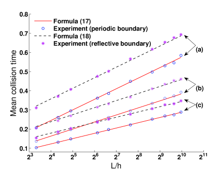
Figure 1: Comparison of the original formula (17) and our revised formula (18) with mean collision time from numerical simulations with periodic and reflective boundary conditions. The two molecules diffuse freely in the 2D domain, with the initial position uniformly distributed in the computational domain. Three parameter sets: (a) $D_{u}=1$, $D_{v}=1$; (b) $D_{u}=2$, $D_{v}=1$; (c) $D_{u}=1$, $D_{v}=3$.

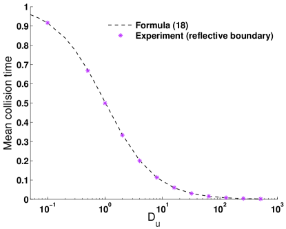
Figure 2: Mean collision times with reflective boundary condition corresponding to different $D_{u}$ values when $D_{v}=1$ is fixed. We use $L=1.0$ and $h=0.01$.

III Mean Reaction Time for Trimolecular Reaction

In this paper, we will first consider periodic boundary conditions and generalize formula (16) to all cases of trimolecular reactions (1)–(3) in one spatial dimension, using both scalings (11) and (13) of reaction rates.

Both trimolecular reactions (1) and (2) are special cases of (3). Since we will focus on the simplified situation where there is only one molecule for each reactant of (3), we may consider (1) as the special case of (3) where diffusion rates for all three molecules are the same, and (2) as the special case where at least two of the three molecules have the same diffusion rates. We will denote the value of mean reaction time by $\tau_{trimol}$. We will decompose $\tau_{trimol}$ into two parts:

$$\tau_{trimol}=\tau_{react}+\tau_{coll},$$ (19)

where $\tau_{react}$ gives the mean time for reaction given that the molecules are initially located in the same compartment, and $\tau_{coll}$ is the mean time for the first collision, i.e. the average time to the state of the system which has all molecules in the same compartment, given that they were initially uniformly distributed. Note that the bimolecular formula (14) was written in the form of a similar decomposition like (19). We will call $\tau_{coll}$ a collision time.

III.1 Special case where $D_{u}=D_{v}$ and $D_{w}=0$

We will start with a simple case with $D_{u}=D_{v}$ and $D_{w}=0$. Then the only $W$ molecule will be fixed at its initial location. Under the periodic boundary condition assumption, without loss of generality, we assume that this $W$ molecule is located at the center of the interval $[0,L]$, or specifically, in the compartment $\left[\frac{K+1}{2}\right]$, where $\left[x\right]$ represents the largest integer that is smaller than $x$. The $U$ and $V$ molecules diffuse according to (7) from their initial compartments. The reaction can fire only when both $U$ and $V$ molecules jump to the center since the only $W$ molecule is at the center. Let $\tau_{coll}$ be the mean time for these two molecules ($U$ and $V$) to be both at the center for the first time, which requires that their compartment number is equal to $\left[\frac{K+1}{2}\right]$.

Instead of trying to develop a formula for the collision time of two molecules diffusing to a fixed compartment in the one-dimensional lattice, we consider an equivalent problem: Imagine a $Z$ molecule jumps with a diffusion rate $D_{u}$ within an $K\times K$ grid in the two-dimensional space and let its compartment index be $z=(x_{1},x_{2})$. Then the two independent random walks by the two $U$ and $V$ molecules in one-dimensional lattice can be viewed equivalently as the random walk of the $Z$ molecule in the two-dimensional square lattice with diffusion rate $D_{u}$. Collision time $\tau_{coll}$ is then equal to the mean time for the pseudo molecule $Z$ to jump to the center for the first time, which is the case discussed in Section II. Therefore, the formula (16) can also be applied to the trimolecular reaction (3) when $D_{w}=0$ and $D_{u}=D_{v}$ and periodic boundary conditions are considered.

III.2 Special case where $D_{u}\neq D_{v}$ and $D_{w}=0$

Formula (16) cannot be directly applied to (3) if $D_{u}\neq D_{v}$ even if $D_{w}=0$. We can still assume $W$ is in the center and consider the equivalent problem of a $Z$ molecule jumps with a diffusion rate $D_{u}$ in the $x$ axis and $D_{v}$ in the $y$ axis within an $K\times K$ grid in the 2D space. The two independent random walks by the two $U$ and $V$ molecules in 1D space can be viewed equivalently as the random walk of the $Z$ molecule in the 2D space with diffusion rate $D_{u}$ and $D_{v}$. We thus introduce the following theorem. The proof can be found in Appendix A.

Theorem 2.

Assume that the molecule $Z$ has a uniformly distributed random starting position in a 2D lattice and that the molecules can move to nearest neighbours only. Assume $Z$ diffuses with diffusion rate $D_{u}$ in the $x$ direction, $D_{v}$ in the $y$ direction, and $D_{u}\geq D_{v}$. Then the following holds:

$$\begin{array}[]{rcl}\tau_{coll}&=&\frac{\displaystyle L^{2}}{\displaystyle 2\pi\sqrt{D_{u}D_{v}}}\log\left(\frac{\displaystyle L}{\displaystyle h}\right)+\frac{\displaystyle L^{2}}{\displaystyle 12D_{v}}\\ &&+\frac{\displaystyle L^{2}}{\displaystyle 4\pi\sqrt{D_{u}D_{v}}}\left[2\left(\gamma+\log\left(\frac{\displaystyle 2}{\displaystyle\pi}\right)\right)-\log\left(1+\frac{\displaystyle D_{u}}{\displaystyle D_{v}}\right)\right],\end{array}$$ (20)

where

$$\gamma=\lim\left(1+\frac{1}{2}+\frac{1}{3}+\cdots+\frac{1}{n}-\log n\right)\approx 0.5772.$$

III.3 Collision time for the general trimolecular reaction

In this subsection we consider the trimolecular reaction (3) with corresponding diffusion rates $D_{u}$, $D_{v}$ and $D_{w}$. Without loss of generality, we assume $D_{u}\geq D_{v}\geq D_{w}>0$.

We consider one pseudo molecule $Z=(z_{1},z_{2})$, where $z_{1}$ and $z_{2}$ are expressed in terms of locations $x_{u}$, $x_{v}$ and $x_{w}$ of three molecules by

$$z_{1}={x_{u}-x_{w}},\quad\mbox{and}\quad z_{2}={x_{v}-x_{w}}.$$ (21)

When $U$, $V$ and $W$ diffuses with rates $D_{u}$, $D_{v}$ and $D_{w}$, the pseudo molecule $Z$ jumps on the 2D lattice corresponding to (21). When $Z$ jumps to the origin, $U$, $V$ and $W$ will be in the same grid, and vice versa. Thus the collision time of the trimolecular reaction in 1D is again converted to the corresponding collision time of the bimolecular problem in 2D. The actual grid and jumps are illustrated in Figure 3.

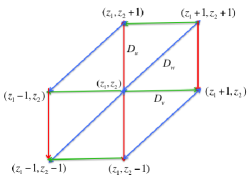
Figure 3: Illustration of the 2D structure for the jumps of $Z$ based on (21). When $U$ molecule jumps, the corresponding $Z$ jumps (shown in red) the direction $(z_{1},z_{2})\longrightarrow(z_{1},z_{2}\pm 1)$. When $V$ molecule jumps, the corresponding $Z$ jumps (shown in green) the direction $(z_{1},z_{2})\longrightarrow(z_{1}\pm 1,z_{2})$; When $W$ molecule jumps, the corresponding $Z$ jumps (shown in blue) the direction $(z_{1},z_{2})\longrightarrow(z_{1}\pm 1,z_{2}\pm 1)$. The whole domain has a similar shape and is not square.

The difficulty of the mapping (21) is that the resulted domain is not square. So we cannot apply the theoretical results presented in the Appendix. In order to apply an estimation on a square lattice, we need to further modify the mapping (21). We will take

$$z_{1}=|x_{u}-x_{w}|,\quad\mbox{and}\quad z_{2}=|x_{v}-x_{w}|.$$ (22)

Then the molecule $Z$ with coordinates $(z_{1},z_{2})$ will jump in an $K\times K$ 2D square lattice, where $K=L/h$. Of course, the jumps at the boundary will be different from the illustration in Figure 3, but that is just symmetric reflection. It does not change the validity of the formula derived in the Appendix, which is based on the assumption of periodic lattices. The domain resulted from the mapping (22) is shown in Figure 4.

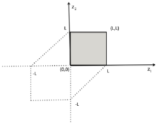
Figure 4: Illustration of the 2D square domain resulted from (22). The original domain (dotted line) resulted from (21) is not square. With (22), the shadowed domain is square and the theoretical analysis in Appendix can be applied.

We have the following approximation formula for the mean jump time.

$$\begin{array}[]{rcl}\tau_{coll}&=&\dfrac{L^{2}}{2\pi\widehat{D}}\log\left(\dfrac{L}{h}\right)+\dfrac{L^{2}}{12\left(D_{v}+D_{w}\right)}\\ &&+\dfrac{L^{2}}{4\pi\widehat{D}}\left[2\Big{(}\gamma+\log\left(\dfrac{2}{\pi}\right)\Big{)}-\log\left(1+\eta^{\prime}\right)\right].\end{array}$$ (23)

where

$$\widehat{D}=\sqrt{D_{u}D_{v}+D_{u}D_{w}+D_{v}D_{w}},$$ (24)

and

$$\eta^{\prime}=\frac{D_{u}^{2}}{{\widehat{D}}^{2}}.$$ (25)

Remark: Formula (23) also implies an estimation of the collision time of bimolecular reaction in a 1D domain. In (23), if we let $D_{u}\longrightarrow\infty$, the formula leads to an estimation of the mean collision time of a bimolecular reaction $V+W\to\emptyset$ in a 1D domain $[0,L]$, which is independent of $h$

$$\tau_{coll}=\frac{L^{2}}{12(D_{v}+D_{w})}.$$ (26)

III.4 Formula under reflective boundary conditions

As shown in Section IV, formula (23) matches with the result computed by stochastic simulations for periodic boundary condition very well. However, when we consider a reflective boundary condition, we see a mismatch. In order to find a formula that matches with the reflective boundary condition results, we performed numerical experiments and collected the mean collision time with reflective boundary conditions. Then with data fitting, we managed to find the formula that matches with numerical results corresponding to reflective boundary conditions. (See Appendix B for derivation of the coefficient of $0.140$.) Equation (27) gives an estimation of the mean first collision time of 1D trimolecular reaction

$$\begin{array}[]{rcl}\tau_{coll}&=&\dfrac{L^{2}}{2\pi\widehat{D}}\log\left(\dfrac{L}{h}\right)+0.140\dfrac{L^{2}}{D_{v}+D_{w}}\\ &&+\dfrac{L^{2}}{4\pi\widehat{D}}\left[2\left(\gamma+\log\left(\dfrac{2}{\pi}\right)\right)-\log\left(0.125+\dfrac{\eta^{\prime}}{4}\right)\right],\end{array}$$ (27)

where $\widehat{D}$ is defined in Equation (24) and $\eta^{\prime}$ is defined in Equation (25).

Remark: When we let $D_{u}\rightarrow\infty$, we have

$$\tau_{coll}=0.14\frac{L^{2}}{D_{v}+D_{w}}.$$ (28)

III.5 Mean Reaction Time

Formula (23) gives the estimation for the mean collision time $\tau_{coll}$ of trimolecular reactions. For the first reaction time $\tau_{trimol}$, since our derivation is based on corresponding analysis on 2D grids, an estimation similar to the equation (14) can be applied. We have

$$\tau_{trimol}\approx\frac{h^{2}(1+N^{1}_{\mathrm{steps}})}{k_{1D}}+\tau_{coll},$$ (29)

as $h\longrightarrow 0$, where $k_{1D}$ is the reaction rate for the trimolecular reaction as defined in (12) and (13).

For biochemical reactions with reflective boundary conditions, we have the formula for the corresponding mean reaction time:

$$\begin{array}[]{rcl}\tau_{trimol}&=&\dfrac{L^{2}}{k_{1D}}+\dfrac{L^{2}}{2\pi\widehat{D}}\log\left(\dfrac{L}{h}\right)+0.140\dfrac{L^{2}}{D_{v}+D_{w}}\\ &&+\dfrac{L^{2}}{4\pi\widehat{D}}\left[2\left(\gamma+\log\left(\dfrac{2}{\pi}\right)\right)-\log\left(0.125+\dfrac{\eta^{\prime}}{4}\right)\right].\end{array}$$ (30)

Correspondingly, if we use the scaling in (11), (30) takes the form

$$\begin{array}[]{rcl}\tau_{trimol}&=&\dfrac{L^{2}h^{4}}{k}+\dfrac{L^{2}}{2\pi\widehat{D}}\log\left(\dfrac{L}{h}\right)+0.140\dfrac{L^{2}}{D_{v}+D_{w}}\\ &&+\dfrac{L^{2}}{4\pi\widehat{D}}\left[2\left(\gamma+\log\left(\dfrac{2}{\pi}\right)\right)-\log\left(0.125+\dfrac{\eta^{\prime}}{4}\right)\right].\end{array}$$ (31)

We can see that as $h\rightarrow 0$, the reaction time will be dominated by the collision time in either case.

IV Numerical Results

We test the collision time of the general trimolecular reaction (3). Figure 5 shows the comparison of the numerical results of the mean first collision time with periodic and reflective boundary conditions with the two formulas (23) and (27). Figure 5 demonstrates that formula (23) matches well with computational results obtained by stochastic simulations corresponding to periodic boundary conditions, justifying our analysis. It also shows that formula (27) matches well with experimental results corresponding to reflective boundary conditions. Figure 6 shows the plot of numerical results of the mean first collision time with periodic and reflective boundary conditions corresponding to different $D_{u}$ when we fix $L$, $D_{v}$ and $D_{w}$. We can see that the two formulas match with the numerical results very well. We also present another comparison and analysis for the special case when $D_{u}\rightarrow\infty$ in Appendix B.

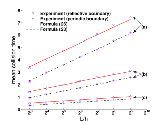
Figure 5: The mean first collision time of three molecules in the 1D domain (for periodic and reflective boundary conditions). The solid lines plot the mean colision time with periodic and reflective boundary conditions corresponding to Formula (23) and Formula (27), while dash lines show the numerical results by stochastic simulations. For the same color from top to bottom, the three sets of diffusion rate parameters are (a) $D_{u}=D_{v}=D_{w}=0.1$; (b) $D_{u}=0.5$, $D_{v}=0.2$, $D_{w}=0.1$ and (c) $D_{u}=2.5$, $D_{v}=0.5$, $D_{w}=0.1$.

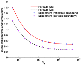
Figure 6: The plot of mean trimolecular collision time (for periodic and reflective boundary conditions) against diffusion rate $D_{u}$. Other parameters are given as $D_{v}=0.2$, $D_{w}=0.1$ and $N=20$. The 1D domain size is fixed at $L=1.0$.

For the mean reaction time comparison, we focus only on reflective boundary condition. In Figure 7, we show the comparison of mean reaction time with formula (30) corresponding to a fix set of diffusion rates and different reaction rates $k_{1D}$.

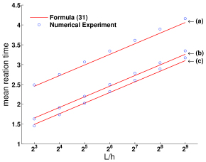
Figure 7: The plot of mean trimolecular reaction time for reflective boundary condition against $\log(L/h)$. The parameters for the plot are $L=1.0,D_{u}=0.5,D_{v}=0.2,D_{w}=0.1$. For the same color, the reaction rates from top to bottom are (a) $k_{1D}=1.0,(b)\ k_{1D}=5.0,(c)\ k_{1D}=25.0$, respectively.

V Discussion

The important consequence of Formula (23) and Formula (27) is that when $h\longrightarrow 0$, $\tau_{coll}\longrightarrow\infty$. Since trimolecular reaction time $\tau_{\mathrm{trimol}}>\tau_{coll}$, the reaction time also tends to infinity. In particular, our analysis confirms the observations made in Oshanin:1995:SAT ; benAvraham:1993:DTR that the diffusion-limited three-body reactions do not recover mean-field mass-action results in 1D. The rate constant in (4) for such problems is time dependent, given by (5), and converges to zero as $t\to\infty$. In the limit $h\to 0$, the average collision time goes to infinity and the rate constant k(t) in (4) converges to zero for any finite time. It is given by (5), where $C\equiv C(h)$ converges to zero as $h\to 0$. In recent years, this topic has been discussed for the bimolecular reaction in the 2D and 3D cases as well. This limitation is a great challenge for spatial stochastic simulation.

Acknowledgments. The research leading to these results has received funding from the European Research Council under the European Community’s Seventh Framework Programme (FP7/2007-2013)/ERC grant agreement n^∘ 239870. Radek Erban would like to thank the Royal Society for a University Research Fellowship and the Leverhulme Trust for a Philip Leverhulme Prize. This work was carried out during the visit of Radek Erban to the Isaac Newton Institute. This work was partially supported by a grant from the Simons Foundation.

Appendix A Formula of Nonuniform Random Walk on a 2D Lattice

We consider the random walk problem on a square 2D lattice. The estimation procedure we present here is generalized from the original idea in Montroll Montroll:1969:RWL . Following the notations in Montroll Montroll:1969:RWL , let $F_{n}(s)$ be the probability that a lattice walker which starts at the origin arrives at a lattice point $s$ for the first time after $n$ steps and

$$F(s,z)=\sum_{n=1}^{\infty}z^{n}F_{n}(s)$$

be the generating function of the set $\{F_{n}(s)\}$. Montroll showed that

$$F(s,z)=[P(s,z)-\delta_{s,0}]/P(0,z),$$

where $P(s,z)$ is the generating function

$$P(s,z)=\sum_{n=0}^{\infty}z^{n}P_{n}(s),$$

where $P_{n}(s)$ is the probability that a walker starting from the origin attires at $s$ for the first time after $n$ steps, no matter how many previous visits he already had at $s$. The generating function for the probability that a walker will be trapped at the origin in a given number of steps is

$$G_{s}(z) = \frac{1}{N-1}\sum_{s\neq 0}F(s,z)$$

$$= \frac{1}{N-1}\left\{\sum_{s}F(s,z)-F(0,z)\right\},$$

where $N=m^{2}$ (with $m=\frac{L}{h}$) is the total number of grids in the square 2D lattice. The average number Montroll:1969:RWL of steps required to reach the origin for the first time is

$$\langle n\rangle = \partial{G_{s}}/\partial{z}|_{z=1}$$ (32)

$$= \frac{1}{N-1}\frac{\partial}{\partial z}\left\{\frac{1}{(1-z)P(0,z)}\right\}_{z=1}.$$

In order to find the formula for $P(0.z)$, the structure function is defined as

$$\lambda(\theta)=\sum_{s}p(s)\exp(i\theta s),$$

where $p(s)$ is the probability that at any step a random walker makes a displacement $s$. $\sum_{s}p(s)=1$. In this 2D square lattice, we consider a general problem. Suppose the random walk can jump to left and right with rate $D_{u}/h^{2}$, to up and down with rate $D_{v}/h^{2}$, and to the diagonal directions with rate $D_{w}/h^{2}$. Let $\sigma_{1}^{2}=\frac{D_{u}}{D_{u}+D_{v}+D_{w}}$, $\sigma_{2}^{2}=\frac{D_{v}}{D_{u}+D_{v}+D_{w}}$, and $\sigma_{3}^{2}=\frac{D_{w}}{D_{u}+D_{v}+D_{w}}$, We thus have

$$\sigma_{1}^{2}+\sigma_{2}^{2}+\sigma_{3}^{2}=1.$$

There are some special cases. In a uniform diffusion case, $\sigma_{1}=\sigma_{2}=\sigma_{3}=\sqrt{3}/3$. In the case $D_{w}=0$, $\sigma_{3}=0$ and then when $\sigma_{1}=\sigma_{2}$, that will be the simple case discussed in Montroll Montroll:1969:RWL . Here we will simply derive the general formula and then discuss different special cases. For the probability $p(s)$ we have $p(1,0)=p(-1,0)=\sigma_{1}^{2}$/2 and $p(0,1)=p(0,-1)=\sigma_{2}^{2}/2$, $p(1,1)=p(-1,-1)=\sigma_{3}^{2}/2$ and

$$\lambda(\sigma)=c_{1}\sigma_{1}^{2}+c_{2}\sigma_{2}^{2}+\sigma_{3}^{2}(c_{1}c_{2}+s_{1}s_{2}),$$

where $\theta=(\theta_{1},\ \theta_{2})$, $c_{i}=\cos\theta_{i}$ and $s_{i}=\sin\theta_{i}$. Then

$$P(0,z)=m^{-2}\sum_{k_{1}=0}^{m-1}\sum_{k_{2}=0}^{m-1}\left[1-z\lambda(2\pi k_{1}/m,2\pi k_{2}/m)\right]^{-1}.$$

In order to obtain $\langle n\rangle$, we need to estimate $P(0,z)$. Following Montroll’s work Montroll:1969:RWL ,

$$P(0,z)=\frac{1}{m}\sum_{k_{1}=0}^{m-1}\left[1-c_{1}\sigma_{1}^{2}z\right]^{-1}f(z,\theta_{1}),$$

where

$$f(z,\theta_{1})=\frac{1}{m}\sum_{k_{2}=0}^{m-1}\left[1-c_{2}w_{1}-w_{2}s_{2}\right]^{-1},$$

with

$$w_{1}=\frac{z(\sigma_{2}^{2}+c_{1}\sigma_{3}^{2}}{1-zc_{1}\sigma_{1}^{2}},$$

and

$$w_{2}=\frac{z(\sigma_{3}^{2}s_{1}}{1-zc_{1}\sigma_{1}^{2}},$$

Following Appendix A of Montroll Montroll:1969:RWL , we define $w_{1}+iw_{2}=\rho e^{i\phi}$. Thus

$$\rho^{2}=w_{1}^{2}+w_{2}^{2}.$$

Then (equation (A7) in Montroll Montroll:1969:RWL )

$$f(z,\theta_{1})=\frac{1}{\sqrt{1-\rho^{2}}}\frac{1-x^{2m}}{1-2x^{m}\cos m\phi+x^{2m}},$$

where $x$ is the smaller root of the equation

$$x^{2}-2x/\rho+1=0.$$ (33)

Now we estimate $P(0,z)$ as

$$P(0,z)=\frac{1}{m}\sum_{k_{1}=0}^{m-1}\left\{\frac{\left(1-zc_{1}\sigma_{1}^{2}\right)^{-1}}{\sqrt{1-\rho^{2}}}\frac{1-x^{2m}}{1-2x^{m}\cos m\phi+x^{2m}}\right\}.$$

First, when $k_{1}=0$, $c_{1}=1$, $s_{1}=0$, $w_{2}=0$ and $\phi=0$. Then

$$\rho=w_{1}=z(1-\sigma_{1}^{2}z)^{-1}(\sigma_{2}^{2}+\sigma_{3}^{2})=\frac{(1-\sigma_{1}^{2})z}{1-\sigma_{1}^{2}z}.$$ (34)

The corresponding term in $P(0,z)$ is given by

$$\begin{array}[]{rcl}&&\frac{1}{m}(1-z\sigma_{1}^{2})^{-1}\frac{1+x^{m}}{1-x^{m}}\left\{1-(\frac{z(1-\sigma_{1}^{2})}{1-z\sigma_{1}^{2}})^{2}\right\}^{-\frac{1}{2}}\\ &=&\frac{1}{m}\frac{1+x^{m}}{1-x^{m}}\left\{(1-z\sigma_{1}^{2})^{2}-z^{2}(1-\sigma_{1}^{2})^{2}\right\}^{-\frac{1}{2}}\\ &=&\frac{1}{m}\frac{1+x^{m}}{1-x^{m}}(1-z)^{-\frac{1}{2}}\left\{1+z-2z\sigma_{1}^{2}\right\}^{-\frac{1}{2}}\\ &=&\frac{1}{m}\frac{1+x^{m}}{1-x^{m}}\frac{1}{\alpha}\left\{2(1-\sigma_{1}^{2})\right\}^{-\frac{1}{2}}\left[1-\beta^{2}(1-2\sigma_{1}^{2})\right]^{-\frac{1}{2}},\end{array}$$

where $\alpha=\sqrt{1-z}$ and $\beta=\frac{\alpha}{\sqrt{2(1-\sigma_{1}^{2})}}$. Now we estimate $x$ defined as in equation (33).

$$\begin{array}[]{rcl}x&=&[1-\sqrt{1-\rho^{2}}]/\rho\\ &=&\frac{1-z\sigma_{1}^{2}-\sqrt{1-z}\sqrt{1+z-2\sigma_{1}^{2}z}}{z(1-\sigma_{1}^{2})}\\ &=&1-2\beta+2\sigma_{1}^{2}\beta^{2}-(2\sigma_{1}^{2}-3)\beta^{3}+\cdots.\end{array}$$

When $m$ is large, we have estimate

$$x^{m}=1-2m\beta+2m^{2}\beta^{2}-4/3m^{3}\beta^{3}+\cdots.$$

Thus

$$(1-x^{m})^{-1}=\frac{1}{2m\beta}\left(1+m\beta+\frac{1}{3}m^{2}\beta^{2}+O(\beta^{3})\right).$$

Then the $k_{1}=0$ term is given by

$$[m^{2}(1-z)]^{-1}+\frac{1}{6(1-\sigma_{1}^{2})}+O(1-z)^{1/2}.$$

For other values of $k_{1}$ as $z\longrightarrow 1$,

$$\begin{array}[]{rcl}&&\left(1-c_{1}\sigma_{1}^{2}\right)\sqrt{1-\rho^{2}}\\ &=&\left[(1-c_{1}\sigma_{1}^{2})^{2}-(\sigma_{2}^{2}+c_{1}\sigma_{3}^{2})^{2}-(\sigma_{3}^{2}s_{1})^{2}\right]^{1/2}\\ &=&\sqrt{1-c_{1}}\left(1-\sigma_{2}^{4}-\sigma_{3}^{4}-c_{1}\sigma_{1}^{4}\right)^{1/2}\\ &=&\sqrt{1-c_{1}}\sqrt{2(\sigma_{1}^{2}\sigma_{2}^{2}+\sigma_{1}^{2}\sigma_{3}^{2}+\sigma_{2}^{2}\sigma_{3}^{2})+\sigma_{1}^{4}(1-c_{1})}\\ &=&2\sqrt{\sigma_{1}^{2}\sigma_{2}^{2}+\sigma_{1}^{2}\sigma_{3}^{2}+\sigma_{2}^{2}\sigma_{3}^{2}}\sin(\pi k_{1}/m)\\ &&\times\left[1+\eta\sin^{2}(\pi k_{1}/m)\right]^{1/2},\end{array}$$

where

$$\eta=\frac{\sigma_{1}^{4}}{\sigma_{1}^{2}\sigma_{2}^{2}+\sigma_{1}^{2}\sigma_{3}^{2}+\sigma_{2}^{2}\sigma_{3}^{2}}.$$ (35)

Thus

$$P(0,z)=[m^{2}(1-z)]^{-1}+\frac{1}{2(1-\sigma_{1}^{2})}\left[\frac{1}{3}+\frac{\phi(0,1)}{r}\right]+O(1-z)^{1/2},$$

where

$$r=\frac{\sqrt{\sigma_{1}^{2}\sigma_{2}^{2}+\sigma_{1}^{2}\sigma_{3}^{2}+\sigma_{2}^{2}\sigma_{3}^{2}}}{1-\sigma_{1}^{2}},$$ (36)

and $\phi(0,1)=S_{1}+S_{2}+S_{3}$ with

$${}S_{1} = \frac{1}{m}\sum_{k=1}^{m-1}\frac{1}{\sin(\pi k/m)},$$

$$S_{2} = \frac{1}{m}\sum_{k=1}^{m-1}\frac{[1+\eta\sin^{2}(\pi k/m)]^{-1/2}-1}{\sin(\pi k/m)},$$

$$S_{3} = \frac{1}{m}\sum_{k=1}^{m-1}\frac{1}{\sin(\pi k/m)}\left\{\frac{2x^{m}(\cos\phi m-x^{m})}{1-2x^{m}\cos\phi m+x^{2m}}\right\}$$

$$\times[1+\eta\sin^{2}(\pi k/m)]^{-1/2}.$$

Following the Appendix A in Montroll Montroll:1969:RWL , there are estimates for $S_{1}$, $S_{2}$.

$$S_{1}=\frac{2}{\pi}\left\{\log m+[\gamma+\log(2/\pi)]-\frac{\pi^{2}}{72m^{2}}+\cdots\right\}.$$

$$S_{2}=-\frac{1}{\pi}\log(1+\eta)+\frac{\eta\pi}{12m^{2}}+\cdots.$$

The estimation for $S_{3}$ is complicated. But fortunately $S_{3}$’s contribution to $P(0,z)$ can be considered small $r$, defined in (36), is not too small. Note that we can obtain an estimation (see Appendix in Montroll Montroll:1969:RWL )

$$x=[1-\sqrt{1-\rho^{2}}]/\rho\approx 1-2rs+2r^{2}s^{2}+\cdots,$$

where $s=\sin\pi k/m$ and $r$ is given in (36). Thus

$$x^{m}\approx e^{-2rsk}(1+O(1/m^{2})).$$

If $r$ is close to zero, $x^{m}$ will be close to one. Then $\frac{x^{m}}{1-x^{m}}$ will be very large, and so will $S_{3}$. But if $r$ is large, $x^{m}$ will be close to zero (except for the term $k=0$) and $S_{3}$ will be small. In order to control the error from the $S_{3}$ term, we always choose $D_{u}$, $D_{v}$ and $D_{w}$ such that $D_{u}\geq D_{v}\geq D_{w}$. In this way $r\geq\left[\frac{\sigma_{1}^{2}}{\sigma_{2}^{2}+\sigma_{3}^{2}}\right]^{1/2}\geq\frac{\sqrt{2}}{2}$ and $S_{3}$ will remains relatively small, when $m$ is large. Thus we will simply disregard the $S_{3}$ term in our formula.

To sum it up, when we choose $\sigma_{1}\geq\sigma_{2}\geq\sigma_{3}$ and considering $N=m^{2}$, we disregard $S_{3}$ and have an estimate of $P(0,z)$ as

$$\begin{array}[]{rcl}P(0,z)&\approx&[N(1-z)]^{-1}+\{c_{1}\log N+c_{2}+c_{3}/N\}\\ &&+O(N^{-2})+O((1-z)^{1/2}),\end{array}$$ (37)

where

$$c_{1} = \frac{1}{2\pi\hat{\sigma}},$$

$$c_{2} = \frac{1}{6(1-\sigma_{1}^{2})}+\frac{1}{2\pi\hat{\sigma}}\left[2(\gamma+\log(2/\pi))-\log(1+\eta)\right],$$

$$c_{3} = \frac{\pi}{24\hat{\sigma}}(\eta-1/3),$$

with

$$\hat{\sigma}=\sqrt{\sigma_{1}^{2}\sigma_{2}^{2}+\sigma_{1}^{2}\sigma_{3}^{2}+\sigma_{2}^{2}\sigma_{3}^{2}},$$

$$\gamma=\lim\left(1+\frac{1}{2}+\frac{1}{3}+\cdots+\frac{1}{n}-\log n\right)\approx 0.5772,$$

and $\eta=\frac{\sigma_{1}^{4}}{\sigma_{1}^{2}\sigma_{2}^{2}+\sigma_{1}^{2}\sigma_{3}^{2}+\sigma_{2}^{2}\sigma_{3}^{2}}$ . According to (32), we have

$$\langle n\rangle=c_{1}N\log N+c_{2}N+c_{3}+O\left(\frac{1}{N}\right).$$ (38)

Now consider the special case $D_{w}=0$. Then $\sigma_{3}=0$ and the domain is really a square lattice. In this case, we have

$$\hat{\sigma}=\sigma_{1}\sigma_{2},$$

$$\eta=\frac{\sigma_{1}^{2}}{\sigma_{2}^{2}},$$

and

$$r=\frac{\sigma_{1}}{\sigma_{2}}.$$

If we select $D_{u}\geq D_{v}$ (thus $\sigma_{1}\geq\sigma_{2}$), $r\geq 1$, the $S_{3}$ term will be relatively small. Then multiply (38) with the average time for each jump $1/k$, where $k=2(D_{u}+D_{v})/h^{2}$, apply $N=(L/h)^{2}$, and disregard lower order terms, we obtain

$$\begin{array}[]{rcl}\tau_{coll}&=&\frac{L^{2}}{2\pi\sqrt{D_{u}D_{v}}}\log\left(\frac{L}{h}\right)+\frac{L^{2}}{12D_{v}}\\ &&+\frac{L^{2}}{4\pi\sqrt{D_{u}D_{v}}}\left[2(\gamma+\log(2/\pi))-\log\left(1+\frac{D_{u}}{D_{v}}\right)\right].\end{array}$$ (39)

If we assume further that $D_{u}=D_{v}$, the equation (39) is close to (16) except a small difference due to the $S_{3}$ term. Note that in this case, the formula (39) is a rigorous estimate.

If $D_{w}\neq 0$, and assume the 2D lattice is square, we let $N=\frac{L^{2}}{h^{2}}$ and multiply (38) with $\frac{h^{2}}{2(D_{u}+D_{v}+D_{w})}$, we end up with a similar estimation

$$\begin{array}[]{rcl}\tau_{coll}&=&\frac{L^{2}}{2\pi\hat{D}}\log\left(\frac{L}{h}\right)+\frac{L^{2}}{12(D_{v}+D_{w})}\\ &&+\frac{L^{2}}{4\pi\hat{D}}\left[2(\gamma+\log(2/\pi))-\log\left(1+\eta^{\prime}\right)\right].\end{array}$$ (40)

where

$$\hat{D}=\sqrt{D_{u}D_{v}+D_{u}D_{w}+D_{v}D_{w}},$$

and

$$\eta^{\prime}=\frac{D_{u}^{2}}{{\hat{D}}^{2}}.$$

Appendix B Special case: $D_{u}\to\infty$

When the diffusion rate of $U$ approaches to infinity, the trimolecular system becomes a bimolecular collision model of $V$ and $W$. The formula (27) gives the mean time for bi-molecular collisions, when $D_{u}\to\infty$:

$$\lim_{D_{u}\to\infty}\tau_{coll}=0.14\frac{L^{2}}{D_{v}+D_{w}}.$$ (41)

In this subsection, we investigate the mean bi-molecular collision time and derive the formula for bi-molecular collision time when the other two molecules have a same diffusion rate $D_{v}=D_{w}$.

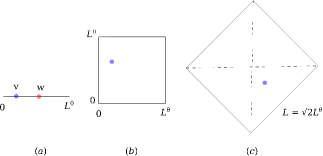
Figure 8: The conversion of the 1D collision model to the first exit time model in 2D domain. (a) The collision model of two molecules $V$ and $W$ freely diffuse in 1D. (b) The diffusion model of one molecule in 2D domain. (c) The first exit model of on molecule in 2D square domain.

Assume a 1D domain of length $L^{\theta}$, two molecules $V$ and $W$ diffuse freely with the rate $D_{v}$ and $D_{w}$ respectively. The 1D diffusion model of two molecules is equivalent to the 2D model in which one molecule diffuses freely with diffusion rates $D_{v}$ and $D_{w}$ in the two directions, independently. The first time for the two molecules to collide in the same position is equivalent to the fist time when the molecule in the 2D domain comes across the diagonal line. With the reflective boundary condition, the triangle domain divided by the diagonal line can be extended into a square domain with the length $L=\sqrt{2}L^{\theta}$. The first encounter time of two molecules on the 1D domain of size $L^{\theta}$ is now converted to a first exit time of on molecule on a 2D domain of size $L=\sqrt{2}L^{\theta}$.

In the following, we derive the formula for the first exit time on the 2D domain. For simplicity, we assume the diffusion rate in the two directions are the same $D=D_{v}=D_{w}$. The Plank-Fokker equation for the diffusion in the 2D domain is given by

$$\frac{\partial}{\partial t}P(\mathbf{x},t|\mathbf{x_{0}},t_{0})=D\Big{(}\frac{\partial^{2}}{\partial x^{2}}+\frac{\partial^{2}}{\partial y^{2}}\Big{)}P(\mathbf{x},t|\mathbf{x_{0}},t_{0}),$$ (42)

with $P(x,t|x_{0},t_{0})$ being the state density function, defined as the probability density that the molecule stays in position $\mathbf{x}$ at time $t$ given it starts from $\mathbf{x_{0}}$ at time $t_{0}$.

Next, we define a probability function

$$G(\mathbf{x_{0}},t;\Omega)\equiv\int_{0}^{L}\int_{0}^{L}dxdyP(\mathbf{x},t|\mathbf{x_{0}},t_{0}),$$ (43)

which describes the probability that the molecule stays in the domain $\Omega=(0,L)\times(0,L)$ at time $t$, given it starts from $\mathbf{x_{0}}$ at time $t=0$. Then, we integrate the Plank-Fokker equation (42) over the 2D interval $\Omega$ and we have the equation for $G$:

$$\frac{\partial}{\partial t}G(x_{0},t;a,b)=D\Big{(}\frac{\partial^{2}}{\partial x^{2}}+\frac{\partial^{2}}{\partial y^{2}}\Big{)}G(x_{0},t;a,b).$$ (44)

The initial condition for the PDE (44) is given as

$$G(\mathbf{x_{0}},0;\Omega)=1.$$ (45)

The four boundaries of the square domain $\Omega$ are all absorbing. Hence, we have the boundary conditions for PDE (44) as

$$\begin{array}[]{rr}G((0,y),t;\Omega)=0;&\quad G((L,y),t;\Omega)=0;\\ G((x,0),t;\Omega)=0;&\quad G((x,L),t;\Omega)=0;\end{array}$$ (46)

Following the definition of $G(\mathbf{x_{0}},t;\Omega)$ (43), $1-G(\mathbf{x_{0}},t;\Omega)$ gives the probability that the molecule exits $\Omega$ before time $t$, which is exactly the distribution function of the first exit time $T(\mathbf{x_{0}};\Omega)$. In addition, the density function of $T(\mathbf{x_{0}};\Omega)$ is given by

$$p(t,\mathbf{x_{0}};\Omega)=\frac{\partial}{\partial t}[1-G(\mathbf{x_{0}},t;\Omega)]=-\frac{\partial}{\partial t}G(\mathbf{x_{0}},t;\Omega),$$ (47)

And the $n$-th moment $T_{n}(\mathbf{x_{0}};\Omega)$ of the random variable $T(\mathbf{x_{0}};\Omega)$ is therefore given by

$$T_{n}(\mathbf{x_{0}};\Omega)=\int_{0}^{\infty}t^{n}\Big{[}-\frac{\partial}{\partial t}G(\mathbf{x_{0}},t;\Omega)\Big{]}dt,(n\geq 0).$$ (48)

For $n=0$, the formula gives

$$T_{0}(\mathbf{x_{0}};\Omega)=-\big{(}G(\mathbf{x_{0}},\infty;\Omega)-G(\mathbf{x_{0}},0;\Omega)\big{)}=1.$$ (49)

Integrating (48) by parts, we get the formula

$$\int_{0}^{\infty}t^{n-1}G(\mathbf{x_{0}},t;\Omega)dt=\frac{1}{n}T_{n}(\mathbf{x_{0}};\Omega)\qquad(n\geq 1).$$ (50)

With equation (47) and (50) we can formulate the moments of $T_{n}(\mathbf{x_{0}};\Omega)$ as coupled ordinary differential equations. Multiply the Plank-Fokker equation (42) through by $t^{n-1}$, integrating the result over all $t$ and substitute from equation (47) and (50), we have the equation

$$-T_{n-1}(\mathbf{x_{0}},\Omega)=D\Big{(}\frac{\partial^{2}}{\partial{x_{0}}^{2}}+\frac{\partial^{2}}{\partial{y_{0}}^{2}}\Big{)}(\frac{1}{n}T_{n}(\mathbf{x_{0}};\Omega)).$$ (51)

The boundary conditions for these differential equations follows the simple derivation from (46) and we have

$$\begin{array}[]{rr}T_{n}((0,y),t;\Omega)=0;&\quad T_{n}((L,y),t;\Omega)=0;\\ T_{n}((x,0),t;\Omega)=0;&\quad T_{n}((x,L),t;\Omega)=0;\end{array}$$ (52)

With the equations ready, we can solve for the moments of the first passage time. Here we are only interested in the first moment and the solution to the PDE of the first moment equation yields

$$\begin{array}[]{rcl}T_{1}(x,y)&=&\displaystyle{\frac{x(L-x)}{2D}-\frac{4L^{2}}{D\pi^{3}}\sum_{k=1,odd}^{\infty}\Big{\{}\frac{\sin(k\pi x/L)}{k^{3}\sinh(k\pi)}}\\ &&\displaystyle{\times\big{(}\sinh(k\pi y/L)+\sinh(k\pi(L-y)/L)\big{)}\Big{\}}}\end{array}$$ (53)

If initially the molecule is homogeneously presented in the square domain, we can calculate the mean first exit time as

$$\begin{array}[]{rcl}<T_{1}>&=&\displaystyle{\frac{1}{L^{2}}\int_{0}^{l}\int_{0}^{1}T_{1}(x,y)dxdy}\\ &=&\displaystyle{\frac{L^{2}}{12D}-\frac{16L^{2}}{D}\sum_{k=1,odd}^{\infty}\frac{\cosh(k\pi)-1}{\pi^{5}k^{5}\sinh(k\pi)}}\\ &\approx&0.0351\displaystyle{\frac{L^{2}}{D}}\end{array}$$ (54)

Therefore, the mean first time when the first two molecules encounter in the 1D domain of size $L^{\theta}$ is exactly the same as the mean first exit time above and the mean first encounter time is given by

$$<T_{coll}>\approx 0.0702\frac{(L^{\theta})^{2}}{D}.$$ (55)

Figure 9 and Figure 10 show the numerical results of the mean first collision time for two molecules with the same diffusion rates and for the general situations. The linear data fitting shows the excellent match with the formula (55). Furthermore, although our derivation is only for the case $D_{v}=D_{w}$, the numerical results show that the first collision time for the general situation, where $D_{v}\neq D_{w}$, follows the similar formula. This formula is given as

$$<T_{coll}>\approx 0.140\frac{(L)^{2}}{D_{v}+D_{w}}.$$ (56)

For comparison purpose, Figure 11 gives the numerical results of the mean first collision time, under periodic boundary condition, for two molecules with different diffusion rates $D_{v}\neq D_{w}$. We can see that the numerical results match with (26) very well.

Figure 9: The mean first collision time of two molecules in the 1D domain with reflective boundary condition, while the two molecules have the same diffusion rate $D=D_{v}=D_{w}$. Other parameters are $N=64$ and $L=0.1$.

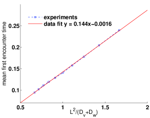
Figure 10: The mean first collision time of two molecules in the 1D domain with reflective boundary condition, while the two molecules have different diffusion rates $D_{v}\neq D_{w}$. Other Parameters are $N=64$ and $L=0.1$.

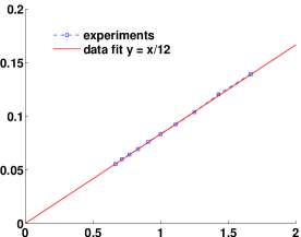
Figure 11: The mean first collision time of two molecules in the 1D domain with periodic boundary condition, while the two molecules have different diffusion rates $D_{v}\neq D_{w}$. Other Parameters are $N=128$ and $L=0.1$.

References

- (1) J. Schnakenberg. Simple chemical reaction systems with limit cycle behaviour. Journal of Theoretical Biology, 81:389–400, 1979.
- (2) F. Schlögl. Chemical reaction models for non-equilibrium phase transitions. Zeitschrift für Physik, 253(2):147–161, 1972.
- (3) L. Qiao, R. Erban, C. Kelley, and I. Kevrekidis. Spatially distributed stochastic systems: Equation-free and equation-assisted preconditioned computation. Journal of Chemical Physics, 125:204108, 2006.
- (4) G. Oshanin, A. Stemmer, S. Luding, and A. Blumen. Smoluchowski approach for three-body reactions in one dimension. Physical Review E, 52(6):5800–5805, 1995.
- (5) T. Plesa, T. Vejchodský, and R. Erban. Chemical reaction systems with a homoclinic bifurcation: an inverse problem. submitted to Mathematical Models and Methods in Applied Sciences, available as http://arxiv.org/abs/1510.07205 , 2015.
- (6) R. Erban, S. J. Chapman, I. Kevrekidis, and T. Vejchodsky. Analysis of a stochastic chemical system close to a SNIPER bifurcation of its mean-field model. SIAM Journal on Applied Mathematics, 70(3):984–1016, 2009.
- (7) J. Paulsson, O. Berg, and M. Ehrenberg. Stochastic focusing: Fluctuation-enhanced sensitivity of intracellular regulation. Proceedings of the National Academy of Sciences USA, 97(13):7148–7153, 2000.
- (8) M. Elowitz, A. Levine, E. Siggia, and P. Swain. Stochastic gene expression in a single cell. Science, 297:1183–1186, 2002.
- (9) D. Gillespie. Exact stochastic simulation of coupled chemical reactions. Journal of Physical Chemistry, 81(25):2340–2361, 1977.
- (10) M. Gibson and J. Bruck. Efficient exact stochastic simulation of chemical systems with many species and many channels. Journal of Physical Chemistry A, 104:1876–1889, 2000.
- (11) Y. Cao, H. Li, and L. Petzold. Efficient formulation of the stochastic simulation algorithm for chemically reacting systems. Journal of Chemical Physics, 121(9):4059–4067, 2004.
- (12) R. Erban, S. J. Chapman, and P. Maini. A practical guide to stochastic simulations of reaction-diffusion processes. 35 pages, available as http://arxiv.org/abs/0704.1908, 2007.
- (13) R. Erban and S. J. Chapman. Reactive boundary conditions for stochastic simulations of reaction-diffusion processes. Physical Biology, 4(1):16–28, 2007.
- (14) S. Andrews and D. Bray. Stochastic simulation of chemical reactions with spatial resolution and single molecule detail. Physical Biology, 1:137–151, 2004.
- (15) K. Takahashi, S. Tanase-Nicola, and P. ten Wolde. Spatio-temporal correlations can drastically change the response of a mapk pathway. PNAS, 107:19820–19825, 2010.
- (16) J. Hattne, D. Fange, and J. Elf. Stochastic reaction-diffusion simulation with MesoRD. Bioinformatics, 21(12):2923–2924, 2005.
- (17) S. Engblom, L. Ferm, A. Hellander, and P. Lötstedt. Simulation of stochastic reaction-diffusion processes on unstructured meshes. SIAM Journal on Scientific Computing, 31:1774–1797, 2009.
- (18) R. Erban. From molecular dynamics to Brownian dynamics. Proceedings of the Royal Society A, 470:20140036, 2014.
- (19) R. Erban. Coupling all-atom molecular dynamics simulations of ions in water with Brownian dynamics. Proceedings of the Royal Society A, Volume 472, Number 2186, 20150556 (2016).
- (20) R. Erban and S. J. Chapman. Stochastic modelling of reaction-diffusion processes: algorithms for bimolecular reactions. Physical Biology, 6(4):046001, 2009.
- (21) I. Agbanusi and S. Isaacson. A comparison of bimolecular reaction models for stochastic reaction-diffusion systems. Bulletin of Mathematical Biology, Volume 76, Number 4, pp. 922-946 (2014).
- (22) M. Flegg. Smoluchowski reaction kinetics for reactions of any order. submitted, available as http://arxiv.org/abs/1511.04786, 2015.
- (23) D. Torney and H. McConnell. Diffusion-limited reactions in one dimension. Journal of Physical Chemistry, 87(11):1941–1951, 1983.
- (24) D. Torney and H. McConnell. Diffusion-limited reaction rate theory for two-dimensional systems. Proceedings of the Royal Society A, 387:147–170, 1983.
- (25) D. ben Avraham. Diffusion-limited three-body reactions in one dimension. Physical Review Letters, 71(24):3733–3735, 1993.
- (26) D. Gillespie. Markov Processes, an introduction for physical scientists. Academic Press, Inc., Harcourt Brace Jovanowich, 1992.
- (27) R. Erban, M. Flegg, and G. Papoian. Multiscale stochastic reaction-diffusion modelling: application to actin dynamics in filopodia. Bulletin of Mathematical Biology, 76(4):799–818, 2014.
- (28) S. Hellander, A. Hellander, and L. Petzold. Reaction-diffusion master equation in the microscopic limit. Physical Review E, 85:042901, 2012.
- (29) E. Montroll. Random walks on lattices. III. Calculation of first-passage times with application to exciton trapping on photosynthetic units. Journal of Mathematical Physics, 10(4):753–765, 1969.