Stellar Mass–Gas-phase Metallicity Relation at $0.5\leq z\leq 0.7$: A Power Law with Increasing Scatter toward the Low-mass Regime

Abstract

We present the stellar mass (${\rm M_{*}}$)–gas-phase metallicity relation (MZR) and its scatter at intermediate redshifts ($0.5\leq z\leq 0.7$) for 1381 field galaxies collected from deep spectroscopic surveys. The star formation rate (SFR) and color at a given ${\rm M_{*}}$ of this magnitude-limited ($R\lesssim 24$ AB) sample are representative of normal star-forming galaxies. For masses below $10^{9}$${\rm M_{\odot}}$, our sample of 237 galaxies is $\sim$10 times larger than those in previous studies beyond the local universe. This huge gain in sample size enables superior constraints on the MZR and its scatter in the low-mass regime. We find a power-law MZR at $10^{8}$${\rm M_{\odot}}$$<$${\rm M_{*}}$$<10^{11}$${\rm M_{\odot}}$: ${\rm 12+log(O/H)=(5.83\pm 0.19)+(0.30\pm 0.02)log(M_{*}/M_{\odot})}$. At $10^{9}$${\rm M_{\odot}}$$<$${\rm M_{*}}$$<10^{10.5}$${\rm M_{\odot}}$, our MZR shows agreement with others measured at similar redshifts in the literature. Our power-law slope is, however, shallower than the extrapolation of the MZRs of others to masses below $10^{9}$${\rm M_{\odot}}$. The SFR dependence of the MZR in our sample is weaker than that found for local galaxies (known as the Fundamental Metallicity Relation). Compared to a variety of theoretical models, the slope of our MZR for low-mass galaxies agrees well with predictions incorporating supernova energy-driven winds. Being robust against currently uncertain metallicity calibrations, the scatter of the MZR serves as a powerful diagnostic of the stochastic history of gas accretion, gas recycling, and star formation of low-mass galaxies. Our major result is that the scatter of our MZR increases as ${\rm M_{*}}$ decreases. Our result implies that either the scatter of the baryonic accretion rate ($\sigma_{\dot{M}}$) or the scatter of the ${\rm M_{*}}$–${\rm M_{halo}}$ relation ($\sigma_{SHMR}$) increases as ${\rm M_{*}}$ decreases. Moreover, our measures of scatter at $z=0.7$ appears consistent with that found for local galaxies. This lack of redshift evolution constrains models of galaxy evolution to have both $\sigma_{\dot{M}}$ and $\sigma_{SHMR}$ remain unchanged from $z=0.7$ to $z=0$.

1. Introduction

The relation between the gas-phase metallicity and stellar mass (${\rm M_{*}}$) of galaxies — ${\rm M_{*}}$–metallicity relation (MZR) — is one of the most fundamental scaling relations of galaxy formation. It is a sensitive tracer of gas inflow, consumption, and outflow, all of which regulate star formation in galaxies.

The MZR in the local universe has been well determined down to ${\rm M_{*}}$$\sim 10^{8}$${\rm M_{\odot}}$ (Tremonti et al., 2004), and has even been explored down to $\sim 10^{6}$${\rm M_{\odot}}$ (Lee et al., 2006). Beyond the local universe, the MZR measurements have been reported up to $z\sim 3$ (e.g., Erb et al., 2006; Maiolino et al., 2008; Zahid et al., 2011; Steidel et al., 2014; Maier et al., 2014; Sanders et al., 2015; Grasshorn Gebhardt et al., 2016). The MZR smoothly evolves from $z>2$ to $z=0$, with lower redshift galaxies having higher metallicity at a given ${\rm M_{*}}$ (e.g., Zahid et al., 2013; Pérez-Montero et al., 2013). Most of the MZR measurements beyond the local universe, however, only explore galaxies with ${\rm M_{*}}$$>10^{9}$${\rm M_{\odot}}$ because spectroscopically observing a sufficiently large sample of low-mass (${\rm M_{*}}$$<10^{9}$${\rm M_{\odot}}$) and thus faint galaxies is very time-consuming.

The sparse number of metallicity measurements of low-mass galaxies beyond the local universe limits our understanding of the redshift evolution of star formation and feedback processes. First, low-mass galaxies are expected to provide the most stringent constraints on feedback because the effect of feedback is expected to be strong in their shallow gravitational potential wells. Second, the scatter of the MZR of low-mass galaxies contains clues on the stochastic nature of the formation mechanisms of low-mass galaxies (Forbes et al., 2014b). Comparing the scatter of low-mass and massive galaxies would tell us whether and by how much the low-mass galaxies are formed through a more stochastic process than massive galaxies.

Feedback processes caused by supernovae (Dekel & Silk, 1986), stellar winds (Hopkins et al., 2012), stellar radiation pressure (Murray et al., 2005), and/or even AGN (Croton et al., 2006) have already become essential ingredients of theories of galaxy formation (see the review of Somerville & Davé, 2015). A complete physical picture of feedback, however, remains to be developed. In recent years, the MZR has been widely used in analytic, semi-analytic, and numerical models to constrain the properties of outflows (e.g., Finlator & Davé, 2008; Peeples & Shankar, 2011; Davé et al., 2011b, a, 2012, 2013; Lilly et al., 2013; Forbes et al., 2014b; Lu et al., 2015a). To understand the redshift evolution of the outflow properties, e.g., the strength, velocity, mass loading factor, metallicity, etc., the MZR measurements at different redshifts are needed.

The observations of the MZR of low-mass galaxies beyond the local universe are sparse. The 26 galaxies of Henry et al. (2013a, H13) comprise the first measurement of the intermediate-redshift MZR below ${\rm 10^{9}M_{\odot}}$. Their MZR is consistent with the equilibrium model with momentum-driven winds (Davé et al., 2012, D12), but their star formation rate (SFR)–${\rm M_{*}}$ relation favors, in contrast, energy-driven winds. It is possible that the equilibrium models endure a breakdown in low-mass galaxies, but the small sample size of H13 also urges the need of large sample to present a robust constraint on the MZR at the low-mass end. Henry et al. (2013b) push the metallicity measurements of low-mass galaxies to higher redshifts at $1.3<z<2.3$ by stacking the Hubble Space Telescope (HST)/WFC3 grism of 83 galaxies in the WISP Survey (Atek et al., 2010; Colbert et al., 2013). Although the stacked spectrum in each ${\rm M_{*}}$ bin has a sufficiently high signal-to-noise ratio (S/N), it loses information of individual galaxies.

The scatter of the MZR of low-mass galaxies beyond the local universe is also unexplored. In the local universe, both Tremonti et al. (2004) and Zahid et al. (2012) observed an increasing scatter as ${\rm M_{*}}$ decreases. In contrast, Lee et al. (2006) found a constant scatter over a 5 dex range of ${\rm M_{*}}$, but their sample size small. While Zahid et al. (2011) provides a robust measurement of the scatter of the MZR at $z\sim 0.8$ with a sufficiently large sample from DEEP2, their sample (${\rm M_{*}}$$>10^{9}$${\rm M_{\odot}}$) does not extend to the low-mass regime.

In this paper, we collect data from large spectroscopic surveys in the CANDELS fields (Grogin et al., 2011; Koekemoer et al., 2011) to study the MZR and its scatter at $0.5\leq z\leq 0.7$ down to ${\rm M_{*}}$$\sim 10^{8}$${\rm M_{\odot}}$. Although none of these surveys (typically limited to $R\lesssim 24.1$) is designed to study low-mass galaxies, each still contains a sufficiently large number of low-mass galaxies. Combining them together provides the largest sample to date in the low-mass regime at $0.5\leq z\leq 0.7$. Recently, extremely metal-poor dwarf galaxies have been found at similar redshifts (e.g., Amorín et al., 2014; Ly et al., 2015), but the main trend and its scatter of the MZR at ${\rm M_{*}}$$<10^{9}$${\rm M_{\odot}}$ is still not well determined.

Table 1Data Summary

Survey	Field	Instrument	Wavelength Range	Resolution	Limiting	Exposure	Number of Galaxies
			(Å)	($R$)	Magnitude	time (hour)	at $0.5\leq z\leq 0.7$a
TKRS (Wirth et al., 2004)	GOODS-N	Keck/DEIMOS	4600–9800	2500	$R\leq 24.4$	1	183 (47/7)
DEEP2 (Newman et al., 2013)	EGS	Keck/DEIMOS	6500–9100	5000	$R\leq 24.1$	1	733 (–/–)
DEEP3 (Cooper et al., 2011, 2012)	EGS	Keck/DEIMOS	4550–9900	2500	$R\leq 24.1$	2	465 (128/55)

Note: ($a$): In each line, the number outside the bracket is the total number of galaxies in our sample. The two numbers within the bracket are the number of galaxies with $10^{8.5}$${\rm M_{\odot}}$$<$${\rm M_{*}}$$\leq 10^{9}$${\rm M_{\odot}}$and the number of galaxies with ${\rm M_{*}}$$\leq 10^{8.5}$${\rm M_{\odot}}$, respectively. For DEEP2, we only use its galaxies with ${\rm M_{*}}$$>10^{9}$${\rm M_{\odot}}$.

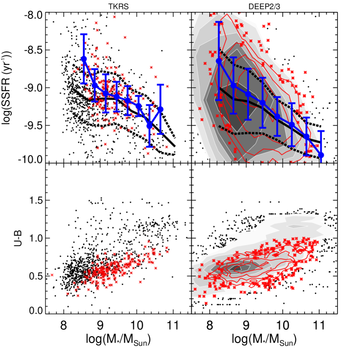
Figure 1.— Sample properties. The SSFR–${\rm M_{*}}$ and U-B color–${\rm M_{*}}$ relations of the galaxies in our sample are plotted as red symbols (plus red contours for DEEP2/3). For each survey (as shown by the title of the upper panels), the mean and 1$\sigma$ scatter of the SSFR–${\rm M_{*}}$ relation of our sample are shown by large blue circles with error bars. Over-plotted black dots (plus gray contours for DEEP2/3) are the mass-complete parent samples, constructed with galaxies with $0.5\leq z\leq 0.7$ and $H<25.0$ from CANDELS/GOODS-N (left column) catalog and $m_{3.6\mu m}<24$ from EGS (right column). The mean and 1$\sigma$ scatter of star-forming galaxies (SSFR$>10^{-10}/yr$) in the parent samples, i.e., the star-forming main sequence at $0.5\leq z\leq 0.7$, are shown by solid and dashed black lines.

We adopt a flat ${\rm\Lambda CDM}$ cosmology with $\Omega_{m}=0.3$, $\Omega_{\Lambda}=0.7$ and the Hubble constant $h\equiv H_{0}/100{\rm km~{}s^{-1}~{}Mpc^{-1}}=0.70$. All magnitudes are on the AB scale (Oke, 1974). The Chabrier (2003) initial mass function is used. The adopted solar metallicity is 12+log(O/H)=8.69 (Allende Prieto et al., 2001; Asplund et al., 2009).

2. Data

Three deep field galaxy spectroscopic surveys are used in this paper: Team Keck Treasury Redshift Survey (TKRS; Wirth et al., 2004), DEEP2 (Newman et al., 2013), and DEEP3 (Cooper et al., 2011, 2012). Since they are well documented and widely discussed in the literature, we only summarize them in Table 1 and refer readers to the survey papers for details.

From each survey, our sample includes only galaxies with reliable spectroscopic redshifts at $0.5\leq z\leq 0.7$ and 3$\sigma$ [OIII] and H$\beta$ detection. To remove AGN contamination, we exclude galaxies that fall in the upper region (main AGN region) of the mass–excitation ([OIII]/H$\beta$ vs. ${\rm M_{*}}$) diagram defined by Juneau et al. (2011). The [OIII]/H$\beta$ metallicity indicator has the issue of the lower–upper branch degeneracy (see Section 3.3). Additional emission lines are needed to break the degeneracy. The effect of the degeneracy on the MZR, however, is believed to be negligible for galaxies with ${\rm M_{*}}$$>$$10^{9}$${\rm M_{\odot}}$ (Zahid et al., 2011, and H13). Therefore, in this mass regime, we use all TKRS, DEEP2, and DEEP3 galaxies, but at ${\rm M_{*}}$$\leq$$10^{9}$${\rm M_{\odot}}$, we only use TKRS and DEEP3 galaxies, which include also [OII] observation to help break the degeneracy. The final sample consists of 1381 galaxies. Among them, 273 galaxies have ${\rm M_{*}}$$<10^{9}M_{\odot}$, comprising a sample $\sim$10 times larger than previous studies in this mass regime at similar redshift (e.g., H13). The numbers of galaxies from each survey are listed in Table 1.

For each galaxy, we fit its multi-wavelength broad-band photometry to synthetic stellar populating models to measure ${\rm M_{*}}$. For TKRS, we use FAST (Kriek et al., 2009) to fit the Bruzual & Charlot (2003) models to CANDELS multi-wavelength catalog (Barro in preparation, see also Guo et al., 2013). For DEEP2/3, we use the EGS multi-wavelength catalog of Barro et al. (2011a), which is constructed based on Spitzer/IRAC 3.6$\mu$m detection. The SED-fitting process, detailed in Barro et al. (2011b), also uses the Bruzual & Charlot (2003) models.

SFRs are measured by following the SFR “ladder” method in Wuyts et al. (2011). This method relies on IR-based SFR estimates for galaxies detected at mid- to far-IR wavelengths, and SED-modeled SFRs for the rest. For IR-detected galaxies the total SFRs (SFR IR+UV) were computed from a combination of IR and rest-frame UV luminosity (uncorrected for extinction) following Kennicutt (1998). For non-IR-detected galaxies, SFRs are measured from the extinction-corrected rest-frame UV luminosity. As shown in Wuyts et al. (2011) the agreement between the two estimates for galaxies with a moderate extinction (faint IR fluxes) ensures the continuity between the different SFR estimates. We refer readers to Barro et al. (2011b, 2013) for the details of our SFR measurements.

An important issue is whether our sample is representative of normal star-forming galaxies, because it is collected from surveys which were not designed to uniformly select low-mass galaxies. Moreover, our S/N threshold on emission lines would introduce the Malmquist bias toward [OIII]- and H$\beta$-bright galaxies. To test how representative our sample is, we compare the ${\rm M_{*}}$–specific SFR (SSFR) and ${\rm M_{*}}$–color relations of our sample to those of a mass-complete sample (parent sample) of the field of each survey at $0.5\leq z\leq 0.7$. For TKRS, we use CANDELS GOODS-N galaxies with $H<25.0$ as the parent samples, which are approximately complete at ${\rm M_{*}}$$>10^{8}M_{\odot}$. For DEEP2/3, we use the IRAC-detected ($m_{3.6\mu m}<24.0$) galaxies at $0.5\leq z\leq 0.7$ from Barro et al. (2011b).

Figure 1 shows that our sample is actually fairly representative of star-forming galaxies, in terms of SSFR and color at a given ${\rm M_{*}}$. The median SSFRs of our TKRS and DEEP2/3 samples match the medians of the GOODS-N and EGS parent samples down to ${\rm M_{*}}$$=10^{9}$${\rm M_{\odot}}$. Below $10^{9}$${\rm M_{\odot}}$, the average SSFR of our sample is slightly higher than that of the star-forming main-sequence at $0.5\leq z\leq 0.7$. At ${\rm M_{*}}$$<10^{9}$${\rm M_{\odot}}$, the median SSFR of our DEEP2/3 sample is higher than that of EGS parent sample by 0.3 dex, which is still less than the scatter of the parent sample (0.5 dex). Since our whole sample is dominated by DEEP2/3 sources, the comparison results of DEEP2/3 (right column of Figure 1) can be treated as being representative of our whole sample. Overall, our sample is representative for normal star-forming galaxies at $0.5\leq z\leq 0.7$, but slightly biased toward high-SSFR galaxies at ${\rm M_{*}}$$<10^{9}$${\rm M_{\odot}}$. This bias is also reflected in the ${\rm M_{*}}$–color diagram, where our sample is biased toward bluer galaxies at ${\rm M_{*}}$$<10^{9}$${\rm M_{\odot}}$. This bias mainly stems from both the R-band selection (rest-frame $\sim$4100Å at these redshifts) of each survey and our requirement of the emission lines to be detected above the 3$\sigma$ level. In Appendix A, we show that neither the S/N cut itself nor the bias toward higher-SSFR galaxies introduces significant systematic offsets to our derived MZR.

3. Metallicity Measurement

3.1. Line Ratio Measurement

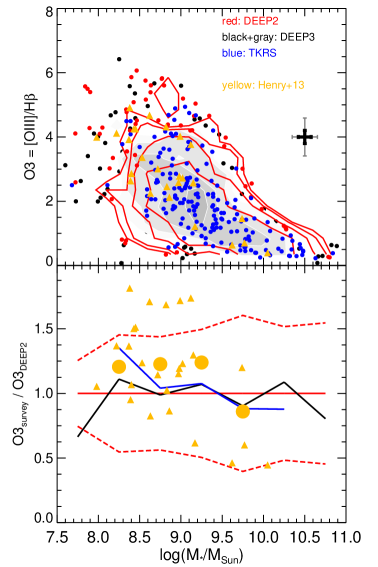
Figure 2.— Upper: [OIII]/H$\beta$ flux ratio as a function of ${\rm M_{*}}$ for galaxies in our sample. Galaxies from different surveys are shown by filled circles with different colors. The DEEP2 (and DEEP3) distribution is shown by red (and gray) contours plus red (and black) circles. The thick black (and thin gray) error bars show the median (and 90 percentile) of the 1$\sigma$ uncertainty of the [OIII]/H$\beta$ and ${\rm M_{*}}$ measurements. For comparison, data of H13 are shown as yellow triangles. Lower: sample-to-sample variation in the [OIII]/H$\beta$ flux ratio. We use our DEEP2 sub-sample as a base sample and show the ratio between the average [OIII]/H$\beta$ of other sub-samples and that of the base sample. The color scheme is the same as that in the upper panel. The base sample (DEEP2) is shown as a constant red solid line at unity, and its 1$\sigma$ confidence level is shown by red dashed lines. H13 data are shown as yellow triangles, while their average values are shown as large yellow circles.

We use the [OIII]/H$\beta$ flux ratio to measure gas-phase metallicity. Unless otherwise noted, [OIII] throughout the paper stands for [OIII]5007Å. A problem of using [OIII]/H$\beta$ to derive the metallicity is its dependence on both the ionization parameter and effective temperature. Another metallicity indicator, R23$\equiv$([OII]3727Å+[OIII]4959,5007Å)/H$\beta$, is often used for optical spectroscopy at similar redshifts. Compared to [OIII]/H$\beta$, R23 has a weaker dependence on the ionization parameter, but it requires an accurate measurement of dust extinction because the extinction is stronger for [OII] than for [OIII]. On the other hand, [OIII]/H$\beta$ is essentially unaffected by dust reddening because the wavelengths of [OIII] and H$\beta$ are quite close. Because only a subset (DEEP3+TKRS) of our sample has [OII] observed, for consistency, we only use R23 to calibrate our metallicity measurement, but use [OIII]/H$\beta$ to derive the metallicity of the whole sample.

To measure the fluxes of [OIII] and H$\beta$ (and [OII] if available), we follow the steps taken by Trump et al. (2013). First, a continuum is fitted across the emission line regions by splining the 50-pixel smoothed continuum. Then, a Gaussian function is fitted to the continuum-subtracted flux in the wavelength regions of the emission lines. The emission line intensities are computed as the area under the best-fit Gaussian in the line wavelength regions. To correct for the stellar absorption of H$\beta$, we follow previous studies with DEIMOS spectra (e.g., Cowie & Barger, 2008; Zahid et al., 2011, and H13) by assuming an equivalent width (EW) of 1$\AA$. We then add the product of the EW and continuum to the H$\beta$ fluxes. The EW correction factor is important for our metallicity measurement. The value of the Hb EW absorption correction depends on the spectral resolution, and studies with lower spectral resolution typically use larger correction factors, e.g., 3 $\AA$ used by Lilly et al. (2003). In Appendix A, we demonstrate that increasing our EW correction to 3 $\AA$ increases the normalization of our derived MZR by 0.1 dex, but does not change its slope and scatter.

The [OIII]/H$\beta$ flux ratio of the whole sample is shown as a function of ${\rm M_{*}}$ in the upper panel of Figure 2. Although galaxies from different surveys have different spectral resolutions and exposure times, they occupy a similar locus in the plot. A more clear view of the sample-to-sample variation is shown in the lower panel of Figure 2. In this panel, we use our DEEP2 sub-sample as a base sample and calculate the ratios of the average [OIII]/H$\beta$ of individual sub-samples to that of the base sample. The comparison results are close to unity in most ${\rm M_{*}}$ bins, suggesting a consistency of line-ratio measurements between the sub-samples with different observational effects.

Each sub-sample only shows deviation from the base sample in its lowest ${\rm M_{*}}$ bin, where the sub-sample is subjected to small number statistics. TKRS deviates from DEEP2 and DEEP3 at $10^{8}$${\rm M_{\odot}}$$<$${\rm M_{*}}$$<10^{8.5}$${\rm M_{\odot}}$, where TKRS only has 7 galaxies, while both DEEP2 and DEEP3 each have around 50 galaxies. The deviation of TKRS does not affect our conclusions in this mass regime. At ${\rm M_{*}}$$<10^{8}$${\rm M_{\odot}}$, both DEEP2 and DEEP3 have only 6-7 galaxies and hence show large discrepancy. In our analyses, we show the results of this mass regime in plots, but do not use them in fitting or to draw any conclusions. Overall, the consistency of line-ratio measurements suggests that our combination of different surveys introduces no significant biases.

The galaxies of H13 (yellow triangles in both panels) provide an independent check on our [OIII]/H$\beta$ measurements. In general, the H13 data follow our main trend. Although the average [OIII]/H$\beta$ of H13 is constantly higher than that of our DEEP2 base sample by a factor of 1.2 at ${\rm M_{*}}$$<10^{9.5}$${\rm M_{\odot}}$, the deviation is still within 1$\sigma$ confidence level of our base sample (red dashed lines). We therefore conclude that our measurements are consistent with those in the literature.

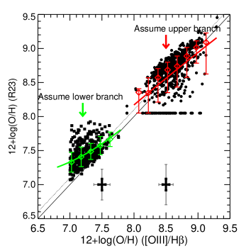
Figure 3.— Comparison between metallicities measured by R23 and [OIII]/H$\beta$ in the DEEP3 sample. Circles (the right locus) show the case of using the upper-branch metallicity values for all galaxies, while squares (the left locus) the lower-branch values. Red (green) diamonds and error bars show the median and 16 and 84 percentiles of the comparison for the upper (lower) branch case. The red (green) curve shows a second-order polynomial fit to the comparison of the upper (lower) branch case. The right and left black (gray) error bars show the median (90 percentile) measurement uncertainty of the upper and lower branches, respectively.

3.2. Metallicity Calibration

The [OIII]/H$\beta$ flux ratio is then converted to metallicity through the calibration of Maiolino et al. (2008, M08). For the low-metallicity regime (12+log(O/H)$<$8.3), M08 calibrate their relations using galaxies with metallicities derived using the electron temperature $T_{e}$ method from Nagao et al. (2006). For high-metallicity galaxies from SDSS DR4, they use the photoionization models of Kewley & Dopita (2002, KD02) to infer metallicity. A polynomial fit is used to connect the low- and high-metallicity galaxies.

We use R23 to calibrate our [OIII]/H$\beta$-derived metallicity. Galaxies in DEEP3 and TKRS comprise a training sample because they have [OII] observed. For each DEEP3 or TKRS galaxy with [OII] S/N$>$3, we measure its R23-derived metallicity with the M08 calibration. When measuring R23, we correct for dust extinctions of [OII], [OIII], and H$\beta$ by converting stellar continuum extinction ${\rm E(B-V)_{*}}$, which is derived through the SED-fitting process performed when measuring ${\rm M_{*}}$ of the galaxies in our sample (see Section 2), into gas extinction ${\rm E(B-V)_{gas}}$ through ${\rm E(B-V)_{gas}=E(B-V)_{*}/0.44}$ (Calzetti et al., 2000).

The comparison between the two metallicities is shown in Figure 3. Both [OIII]/H$\beta$ and R23 face the issue of non-unique metallicity solutions, i.e, a given line ratio has two solutions: a lower-metallicity value (lower branch) and a higher-metallicity one (upper branch). For each galaxy here, we compare its solution in the same branch of [OIII]/H$\beta$ and R23, i.e., upper vs. upper (circles in the panel) and lower vs. lower (squares). We will break the branch degeneracy for each galaxy later.

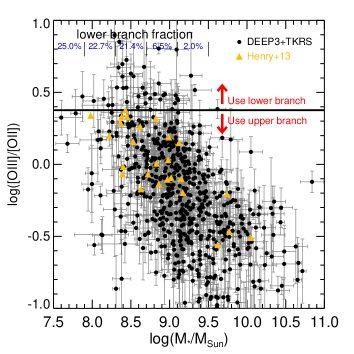
Figure 4.— Using [OIII]/[OII] to break the lower–upper branch degeneracy in the DEEP3+TKRS training sample. Each black circle with gray error bars shows one galaxy. Galaxies above log([OIII]/[OII])=0.375 (black horizontal line) are identified to use their lower-branch metallicities, and vice versa. In each mass bin (width of 0.4 dex), the fraction of galaxies in the lower branch is given by the blue number in top. For comparison, data of H13 are shown as yellow triangles.

The average deviation between the two metallicities is about 0.1 dex for the upper branch solutions. For the lower branch, the deviation increases as the metallicity decreases, from $\sim$0.1 dex at 12+log(O/H)=7.5 to $\sim$0.3 at 12+log(O/H)=7.0. We will show later, however, that no galaxies would take a lower-branch solution smaller than 12+log(O/H)=7.3 when we break the degeneracy. We fit a second-order polynomial function to the Z(R23)–Z([OIII]/H$\beta$) relation of the upper branch (red curves) and lower branch (green curves), respectively. We then use the best-fit relation to correct the [OIII]/H$\beta$-derived metallicities — both the upper- and lower-branch solutions — of all the galaxies in the three surveys, regardless of whether they have [OII] observations.

3.3. Breaking the Upper–Lower Branch Degeneracy

To break the degeneracy between the two branches, we use the DEEP3+TKRS galaxies as a training sample, where both [OII] and [OIII] are observed. As shown by M08, [OIII]/[OII] decreases monotonically with metallicity and hence can be used as an indicator to break the degeneracy. H13 showed that ([OIII]4959,5007Å)/[OII]$>$3.0 works as a reasonable threshold to identify lower-branch galaxies. The threshold of 3.0 corresponds to 12+log(O/H)$\sim$8.0 (M08), which is the turnover point of the two branches of [OIII]/H$\beta$. We assume a flux ratio [OIII]4959Å:[OIII]5007Å=1:3, so our threshold is log([OIII]/[OII])=0.375 (the horizontal line in Figure 4). Galaxies with log([OIII]/[OII])$>$0.375 are identified to be in the lower branch, and vice versa . For each ${\rm M_{*}}$ bin, we calculate the fraction of galaxies that are in the lower branch. At ${\rm M_{*}}$$>10^{9}$${\rm M_{\odot}}$, only 2% of the galaxies are in the lower branch. This is consistent with the fact that, although galaxies with very low metallicity have been found at $z\sim 0.7$ (Hoyos et al., 2005; Amorín et al., 2014; Ly et al., 2014, 2015), their number densities are quite low. But the fraction increases toward lower ${\rm M_{*}}$, and about 25% of the galaxies at ${\rm M_{*}}$$<10^{8.3}$${\rm M_{\odot}}$ are in the lower branch. Henry et al. (2013b) find a turnover of the R23–${\rm M_{*}}$ relation at ${\rm M_{*}}$$\sim 10^{8.5}$${\rm M_{\odot}}$ in their stacked HST/WFC3 grism spectra. Although they cannot break the degeneracy for individual galaxies because of using the stacked spectra, their result suggests that the lower-branch fraction becomes larger when ${\rm M_{*}}$ decreases and that the majority of low-mass galaxies are in the lower branch.

The above [OIII]/[OII] threshold and thus determined lower-branch fraction are only valid for our metallicity indicator [OIII]/H$\beta$ in the M08 calibration. The “turnover” point of the two branches is different for different metallicity indicators and calibrations. For example, for [OIII]/H$\beta$ in M08, the turnover point is around 12+log(O/H)$\sim$8.0 (see Figure 5 of M08), but for R23 in KD02, the turnover point is around 12+log(O/H)$\sim$8.4. Therefore, galaxies with 12+log(O/H)=8.0–8.4 would be in the upper branch of our [OIII]/H$\beta$ but in the lower branch of R23 of KD02. This difference can explain the discrepancy between our lower-branch fraction and that of other studies with different metallicity indicators. For example, Maier et al. (2015) find a higher fraction of lower-branch galaxies at ${\rm M_{*}}$$>10^{9.5}$${\rm M_{\odot}}$ using R23 of KD02. The lowest metallicity in Maier et al. (2015) is around 12+log(O/H)$\sim$8.3, which is still in the upper branch of [OIII]/H$\beta$. Therefore, we expect to find no object in our [OIII]/H$\beta$ lower-branch at this mass regime. Figure 4 confirms our expectation by showing no galaxies with [OIII]/[OII]$>$0.375 at ${\rm M_{*}}$$>10^{9.5}$${\rm M_{\odot}}$. In this sense, our results are consistent with Maier et al. (2015).

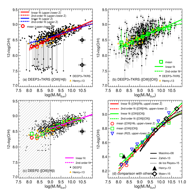
Figure 5.— (a): MZR of our DEEP3+TKRS sample with metallicity measured through [OIII]/H$\beta$. Black circles are the metallicity of each galaxy after breaking the lower–upper branch degeneracy using the threshold in Figure 4. For each lower-branch galaxy, we also show its upper-branch metallicity by a gray circle and connect it to its lower-branch metallicity with a gray vertical line. The means, best linear fit, and best second-order polynomial fit of the metallicity after breaking the degeneracy (“upper+lower Z”) are shown by red open circles, solid line, and dashed line. As a reference, the blue solid and dashed lines show the best linear and second-order polynomial fits of the sample using the upper-branch metallicities (“upper Z”) for all galaxies. The upper and lower black (gray) error bars show the median (90 percentile) measurement uncertainty of the upper and lower branches, respectively. (b): MZR of our DEEP3+TKRS sample with metallicity measured through [OIII]/[OII]. The means, best linear fit, best second-order polynomial fit are shown by green open squares, solid line, and dashed line. (c): MZR of our DEEP2 sample with metallicity measured through [OIII]/H$\beta$. All galaxies use their “upper Z”. Galaxies at ${\rm M_{*}}$$<10^{9}$${\rm M_{\odot}}$ (shaded area) are significantly subjected to the branch degeneracy and hence not used in our analyses. The best linear and second-order polynomial fits are shown by purple solid and dashed lines. The means of DEEP3+TKRS are shown as open circles ([OIII]/H$\beta$-derived “upper+lower Z”) and squares ([OIII]/[OII]-derived). Data from H13, after being converted to the M08 metallicity calibration, are shown as yellow triangles in Panel (a), (b), and (c). (d): Comparison between our MZRs and other measurements in the literature. Red and green lines and symbols are the same as in Panel (a), (b), and (c). We also add the mean metallicity measured through R23 in this panel (blue triangles). Black curves and symbols show the MZRs at similar redshifts from other studies, as the labels indicate. The y-axis range of Panel (d) is different from that of other panels.

4. Stellar Mass–Metallicity Relation at $0.5\leq z\leq 0.7$

4.1. Stellar Mass–Metallicity Relation at $0.5\leq z\leq 0.7$

Table 2Best-fit Parameters of the MZR: $12+{\rm log(O/H)}=c_{0}+c_{1}{\rm log(M_{*}/M_{\odot})}+c_{2}{\rm log(M_{*}/M_{\odot})}^{2}$

Samplea	Line ratio	Branch Degeneracyb	$c_{0}$	$c_{1}$	$c_{2}$	fiducial relationc
DEEP3+TKRS	[OIII]/H$\beta$	upper+lower Z	$5.83\pm 0.19$	$0.30\pm 0.02$	fixed to 0	Yes
DEEP3+TKRS	[OIII]/H$\beta$	upper+lower Z	$2.64\pm 2.35$	$0.98\pm 0.51$	$-0.04\pm 0.03$
DEEP3+TKRS	[OIII]/H$\beta$	upper Z	$6.70\pm 0.09$	$0.21\pm 0.02$	fixed to 0
DEEP3+TKRS	[OIII]/H$\beta$	upper Z	$9.48\pm 1.20$	$-0.39\pm 0.26$	$0.03\pm 0.02$
DEEP3+TKRS	[OIII]/[OII]	—	$5.90\pm 0.18$	$0.30\pm 0.02$	fixed to 0
DEEP3+TKRS	[OIII]/[OII]	—	$1.65\pm 2.34$	$1.21\pm 0.51$	$-0.05\pm 0.03$
DEEP2	[OIII]/H$\beta$	upper Z	$6.57\pm 0.11$	$0.23\pm 0.02$	fixed to 0
DEEP2	[OIII]/H$\beta$	upper Z	$7.53\pm 2.40$	$0.03\pm 0.50$	$0.01\pm 0.03$

Note: ($a$): DEEP3+TKRS galaxies have [OII] measurements to allow breaking the lower–upper branch degeneracy. DEEP2 galaxies have no [OII] measurements. We therefore only fit the DEEP2 MZR with galaxies at ${\rm M_{*}}$$\geq 10^{9}$${\rm M_{\odot}}$, where the fraction of galaxies in the lower branch is negligible. ($b$): This column indicates whether we break the lower–upper branch degeneracy. “upper+lower Z” uses the metallicity values after breaking the lower–upper branch degeneracy using the [OIII]/[OII] threshold in Figure 4. “upper Z” does not break the degeneracy and uses the upper-branch metallicity for all galaxies. There is no branch degeneracy issue for the metallicity measured through [OIII]/[OII]. ($c$): The fiducial MZR relation is used in our comparisons with other MZR measurements and models.

We first measure the MZR of the DEEP3+TKRS sample, in which each galaxy breaks the lower–upper branch degeneracy by using the [OIII]/[OII] threshold. The MZR (called “upper+lower Z” hereafter) is shown in Panel (a) of Figure 5. For each galaxy with log([OIII]/[OII])$>$0.375, we connect its lower branch (black circle) and upper branch (gray circle) metallicities with a gray vertical line to show the difference between the two solutions. For these galaxies, we use their lower-branch solutions when deriving the MZR, while for other galaxies, we use their upper-branch solutions.

We fit a polynomial function to the DEEP3+TKRS “upper+lower Z” MZR:

$$12+{\rm log(O/H)}=c_{0}+c_{1}x+c_{2}x^{2},$$ (1)

where $x={\rm log(M_{*}/M_{\odot})}$. This function becomes a linear function when $c_{2}=0$. The best-fit parameters, with either a free $c_{2}$ or a fixed $c_{2}=0$, are shown in Table 2.

The second-order polynomial fit (red dashed line in Panel (a)) shows almost no difference from the linear fit (red solid line), except at the very massive end. The $\chi^{2}$ value of the polynomial fit is comparable to that of the linear fit, but an $F$-test shows that the former does not significantly improve the goodness-of-fit by adding one more free parameter. Therefore, we choose the linear fit as our preferred function. The linear DEEP3+TKRS MZR has a slope of $0.30\pm 0.02$. For a comparison, we also measure the MZR by using the upper branch solutions for all galaxies. Not surprisingly, the fits (blue solid and dashed lines and parameters of “upper Z” in Table 2) show a flatter slope at the low-mass end.

Panel (a) shows a gap in the metallicity distribution at ${\rm M_{*}}$$<10^{9.5}$${\rm M_{\odot}}$. This gap exists because we only allow each galaxy to use one metallicity from its upper- and lower-branch values. The discreteness of the two branches results in the gap. For example, in Panel (a), a galaxy whose upper and lower branch metallicities are connected by a vertical gray line can only choose either of its two endpoints but no other values. This gap is a generic feature of some metallicity calibrations when breaking the degeneracy. It is independent on which emission lines are used to measure the metallicity. A similar gap also exists even if we use the M08 calibration of the R23 indicator. Similar gaps from different line ratios and calibrations can be seen from Panel (3), (4), and (5) of Figure 1 of Kewley & Ellison (2008).

Choosing one value from the two branches is a deterministic method, which over-simplifies the metallicity calibration in the “turnover” region by not taking into account of the dispersion (or uncertainty) of the calibration. For example, the [OIII]/H$\beta$–-metallicity calibration used in our paper, namely the “best-fit” relation of M08, has been shown to have a dispersion of about 0.15 dex in [OIII]/H$\beta$ at a given metallicity (Figure 5 of M08 and Figure 17 of Nagao et al. (2006)). This dispersion (either intrinsic or due to measurement uncertainties), when being converted into the dispersion of metallicity at a given emission-line ratio, would cause the emission-line ratios to lose their diagnostic powers in the “turnover” region: a wide range of metallicity may have the same emission-line ratio (see Figure 11 of Kewley & Ellison (2008) for an example of R23). In principle, this dispersion should be taken into account when converting emission-line ratios into metallicity. This step, however, requires that the dispersion is measured from a sample of galaxies that matches the properties of our sample of interest. Because of the lack of such a sample at our target redshift, we skip this step and retrograde to the deterministic method. We then test its effect on our MZR measurement.

To test the effect of the gap, we need an indicator that changes monotonically with metallicity to provide an independent check. [NII]/H$\alpha$ is usually the first choice for lower-redshift galaxies, but it is shifted out of the wavelength window of our data. Here, we use [OIII]/[OII] as the independent check. Although [OIII]/[OII] is in fact a diagnostic of ionization parameter, it also provides a sort of metallicity measurement, thanks to the tight relation between ionization parameter and metallicity (see Nagao et al., 2006, for detailed discussions). The tight relation between ionization parameter and metallicity is also manifested by the tight locus of star-forming main sequence galaxies in the BPT diagrams (e.g., Cid Fernandes et al., 2007; Kewley et al., 2013; Maier et al., 2015). We use the calibration of M08 to convert [OIII]/[OII] to metallicity. Grasshorn Gebhardt et al. (2016) shows that the calibration evolves little from M08’s local sample to their z$\sim$2 sample.

The new MZR is shown in Panel (b) of Figure 5. There is no gap of metallicity in this panel, although the scatter is increased. The mean relation and 1$\sigma$ deviation (green squares with error bars) agree very well with the data points of H13, which are measured through R23. This comparison ensures that using [OIII]/[OII] is able to recover the mean metallicity at each ${\rm M_{*}}$ bin. Also, the comparison between the best-fit relations of the [OIII]/H$\beta$-derived and [OIII]/[OII]-derived MZRs (red and green lines in Panel (d)) shows only small systematic offset of $\sim$0.05 dex in normalization and no changes at all in slope. Such good agreement demonstrates that our method of breaking the branch degeneracy introduces no significant effects on both the slope and the normalization of the MZR. We therefore use the “upper+lower Z” MZR as our fiducial one to compare with other measurements and models later.

In Panel (d) of Figure 5, we also show the mean metallicity of each ${\rm M_{*}}$ bin by using the R23 indicator of M08 (blue triangles). The upper–lower degeneracy is also broken by using the same [OIII]/[OII] threshold in Figure 4. The mean R23 metallicity shows very small deviation from our mean [OIII]/H$\beta$-derived metallicity. This result again demonstrates that the slope and normalization of our MZR derived through [OIII]/H$\beta$-derived are robust.

To provide a better statistics, we also measure the MZR of our DEEP2 sample through [OIII]/H$\beta$. Since we do not have [OII] observation for DEEP2 galaxies, we are not able to break the branch degeneracy. We therefore only measure the DEEP2 MZR down to $10^{9}$${\rm M_{\odot}}$ because, as shown by the lower-branch fraction of DEEP3+TKRS in Figure 4, the number of lower-branch galaxies is negligible in the massive and intermediate-mass regimes. For galaxies at ${\rm M_{*}}$$>10^{9}$${\rm M_{\odot}}$, the DEEP2 mean MZR matches that of DEEP3+TKRS (both [OIII]/H$\beta$ and [OIII]/[OII] derived) very well (Panel (c) of Figure 5).

4.2. Comparison with Other MZRs

Our fiducial MZR (“upper+lower Z”) at ${\rm M_{*}}$$>10^{9}$${\rm M_{\odot}}$ shows good agreement with other measurements at similar redshifts in the literature. Panel (d) of Figure 5 shows the MZRs of M08, Zahid et al. (2013), de los Reyes et al. (2015), and Maier et al. (2015), all converted to the calibration of KD02 (the same calibration used in M08 for high-metallicity galaxies) using the calibration conversion table of Kewley & Ellison (2008). At $10^{9}$${\rm M_{\odot}}$$<$${\rm M_{*}}$$<10^{10.5}$${\rm M_{\odot}}$, other MZRs show a deviation of only $<$0.05 dex from ours, which is much smaller than the scatter of our sample. At ${\rm M_{*}}$$<10^{9}$${\rm M_{\odot}}$, the average metallicity of H13 (also converted to the calibration of M08) is higher than our best-fit MZR by $\sim$0.1 dex at ${\rm M_{*}}$$<10^{8.5}$${\rm M_{\odot}}$, which can be attributed to the fact that H13 assumes all galaxies being in the upper branch.

Although the absolute metallicity values of our sample in the intermediate ${\rm M_{*}}$ range match other studies, the slope of our MZR is different from that of others. Because we prefer a linear fit, our slope is constant ($0.30\pm 0.02$) across the 3-dex range of the ${\rm M_{*}}$. This result appears in contrast to the “saturation” of metallicities in massive galaxies found by other authors, e.g., M08, Zahid et al. (2013), and de los Reyes et al. (2015), who found that the slope of MZR decreases significantly as ${\rm M_{*}}$ increases. The different slopes between our and other studies at the massive end could be attributed to a few reasons.

First, we do not have enough massive galaxies at ${\rm M_{*}}$$>10^{10.5}M_{\odot}$ to constrain the slope at the massive end (only 19 in our whole sample). Second, the slope of the massive end is sensitive to AGN removal. AGN contamination would bias the average metallicity of massive galaxies toward lower values because the strong [OIII] emission of AGN host galaxies would make the galaxies resemble a low-metallicity galaxies with higher [OIII]/H$\beta$. We use the mass-excitation method to exclude both X-ray and non-X-ray AGN, but some studies, e.g., Zahid et al. (2013), only exclude X-ray AGN (see Appendix B for detailed discussions of AGN removal). Third, the analytic functions used to fit the MZR are different. Other studies use second-order polynomial functions (M08 and de los Reyes et al. (2015)) or power-law (Zahid et al., 2013) to fit the MZR in logarithmic space. As show in Table 2, the second-order polynomial fits to our [OIII]/H$\beta$ “upper+lower Z” and [OIII]/[OII] MZRs have $c_{2}<0$, indicating a slight “saturation” at ${\rm M_{*}}$$>10^{10.5}M_{\odot}$. These polynomial fits (red and green dashed lines in Panel (d)) actually match the MZR of M08 and de los Reyes et al. (2015) very well.

At the low-mass end, we find a high average metallicity compared to the extrapolation of other MZR relations to ${\rm M_{*}}$$\sim 10^{8}M_{\odot}$ (i.e., extrapolating all black lines in Panel (b) of Figure 5 to low mass). The slope and normalization of our MZR at the low-mass end do not significantly depend on the choice of fitting functions. Other studies have almost no data at ${\rm M_{*}}$$<10^{9}$${\rm M_{\odot}}$ to constrain the slope at the low-mass end. The good agreement between our MZR and that of H13 at the low-mass end (Panel (d) of Figure 5) provides reassurance to our measurement. We therefore believe that simply extrapolating other MZRs to the low-mass regime would underestimate the average metallicity of galaxies with ${\rm M_{*}}$$<10^{9}$${\rm M_{\odot}}$.

Our sample selection would not bias our MZR at the low-mass end. As shown in Section 2, our sample is quite representative in terms of SSFR and U-B color at a given ${\rm M_{*}}$ down to ${\rm M_{*}}$$\sim 10^{9}M_{\odot}$. Below that, our sample is biased toward galaxies with higher SSFR (and hence bluer color). If the local SFR dependence, i.e.,at a given ${\rm M_{*}}$, lower SFR galaxies having higher metallicity, is also found in our sample, we would expect that our average metallicity at ${\rm M_{*}}$$<10^{9}M_{\odot}$ is underestimated instead of overestimated, which suggests that the true MZR may be even flatter than what we find. As shown in Section 4.3, however, we only find a very weak SFR dependence of metallicity in our sample, which would not significantly bias our MZR measurement. In fact, detailed tests in Appendix A show that sample selection (in SSFR and emission-line S/N) has no significant effects on our derived MZR. Our sample selection would bias the MZR toward higher metallicity only if a positive SFR dependence, i.e., galaxies with higher SFR having higher metallicity (Ly et al., 2014), holds at $0.5\leq z\leq 0.7$.

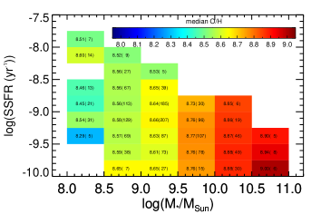
Figure 6.— SSFR dependence of the MZR. The median metallicity of each (${\rm M_{*}}$, SSFR) bin is shown by color, with the color bar in the upper right part. The median metallicity value as well as the number of galaxies in each bin are also given. Each bin spans 0.5 dex in ${\rm M_{*}}$ and 0.25 dex in SSFR.

4.3. Weak SSFR Dependence

Local galaxies are shown to follow a fundamental metallicity relation (Mannucci et al., 2010, 2011): at a given ${\rm M_{*}}$, galaxies with higher SFR have lower metallicity, and vice versa. The ${\rm M_{*}}$–SFR–metallicity surface (or fundamental metallicity plane, FMR) can be collapsed to a two-dimensional space by relating metallicity to a linear combination of ${\rm M_{*}}$ and SFR. Mannucci et al. (2011) demonstrate that metallicity correlates tightly with the quantity $\mu_{0.32}=\log(M_{*})-0.32*\log(SFR)$ (in solar units) down to ${\rm M_{*}}$$\sim 10^{9.2}$${\rm M_{\odot}}$. To test the SFR dependence of the MZR in our sample, we measure the median metallicity of each (${\rm M_{*}}$, SSFR) bin and show the results in Figure 6. At a given ${\rm M_{*}}$, SSFR and SFR are equivalent. We choose the SSFR–${\rm M_{*}}$ space rather than the SFR–${\rm M_{*}}$ space because the former is used to show our sample selection effect in Section 2. The figure is similar to and enables an easy comparison with the representation of metallicities in the color-coded SSFR–${\rm M_{*}}$ diagram in Maier et al. (2015) (their Figure 4). We use the upper-branch [OIII]/H$\beta$-derived metallicities of all DEEP3+TKRS and DEEP2 galaxies for this test. Since we only present the median metallicity, given the small fraction of lower-branch galaxies ($<$30% in even the lowest ${\rm M_{*}}$ bin), not identifying lower-branch galaxies would not affect the median metallicities.

The SSFR (or SFR) dependence of metallicity in our sample is weak. Our strongest signal is from galaxies with $10^{8.5}$${\rm M_{\odot}}$$<$${\rm M_{*}}$$<$$10^{9.5}$${\rm M_{\odot}}$. In this regime, the metallicity decreases by at most 0.15 dex when log(SSFR/yr) increases from -10 to -8. As a comparison, Mannucci et al. (2010) (see their Fig. 6) find that for local galaxies at the same ${\rm M_{*}}$ range, the metallicity changes by 0.3 dex from log(SSFR/yr)=-10 to -9 and would change by $\sim$0.6 dex from log(SSFR/yr)=-10 to -8 with extrapolation.

Our result is consistent with that of de los Reyes et al. (2015) and Pérez-Montero et al. (2013), both in favor of a moderate or no SFR dependence of the MZR at similar redshifts. In contrast, some other studies (e.g., Cresci et al., 2012; Maier et al., 2015) find a SFR dependence at $z\sim 0.7$ as strong as in local galaxies (i.e., a non-evolved FMR between $z\sim 0$ and $z\sim 0.7$). The discrepancy indicates the uncertainty of the existence of a fundamental metallicity relation beyond the local universe. The weaker SFR dependence could be a physical phenomenon at intermediate redshift, suggesting that galaxies need time to establish the SFR dependence of their metallicity. This speculation is consistent with the results at even higher redshifts from Steidel et al. (2014), Sanders et al. (2015), and Grasshorn Gebhardt et al. (2016), who find no SFR dependence of the MZR at z$\sim$2. But the lack of SFR dependence could also be due to selection effects. Mock observations by using local galaxies with strong SFR dependence to mimic high-redshift observations are needed to test the selection effects (Salim et al., 2015).

Figure 7.— Scatter of the MZR of our sample. Scatter is defined as the half-width between the 84th and 16th percentiles (${\rm P_{84}}$ and ${\rm P_{16}}$) of the metallicity distribution at a given ${\rm M_{*}}$. Left (a): Observed scatter. Measurements from different samples and/or different methods of breaking the lower–upper branch degeneracy are plotted with different symbols as the labels show. We only measure the scatter of DEEP2 down to ${\rm M_{*}}$=$10^{9}$${\rm M_{\odot}}$. The solid black line shows the scatter of Zahid et al. (2011) at $z\sim 0.8$ from DEEP2 data. Right (b): Intrinsic scatter. The measurement uncertainties are subtracted from the observed scatter in quadrature. Symbols have the same meaning as in Panel (a). A third-order polynomial function is fitted to our measurements: red squares, green circles, and purple diamonds at ${\rm M_{*}}$$\geq 10^{9}$${\rm M_{\odot}}$ and only green circles at ${\rm M_{*}}$$\leq 10^{9}$${\rm M_{\odot}}$. The scatter of local MZRs of Tremonti et al. (2004) and Zahid et al. (2012) are shown by solid and dashed black lines. The scatter from the initial and improved guesses of Forbes et al. (2014b) are shown by dashed–dotted and dotted gray lines. The scatter of numerical simulations of Davé et al. (2013) is shown by the solid gray line.

5. Scatter of the MZR

Our $\sim$10-fold gain in sample size enables a solid study of the scatter of the MZR at the low-mass end at $0.5\leq z\leq 0.7$ for the first time. Figure 7 shows the scatter of the MZR of our sample. We define the scatter as the half width between the 84th and 16th percentiles (${\rm P_{84}}$ and ${\rm P_{16}}$) of the metallicity distribution at a given ${\rm M_{*}}$.

We measure the scatter for our four MZRs: (1) DEEP3+TKRS [OIII]/H$\beta$-derived “upper+lower Z”, (2) DEEP3+TKRS [OIII]/H$\beta$-derived “upper Z”, (3) DEEP3+TKRS [OIII]/[OII]-derived, and (4) DEEP2 [OIII]/H$\beta$-derived. The results are shown by different symbols in Figure 7. The DEEP3+TKRS [OIII]/H$\beta$-derived “upper Z” scatter can be treated as a lower limit of the MZR scatter because putting all galaxies in the upper branch artificially reduces the MZR scatter. The DEEP3+TKRS [OIII]/H$\beta$-derived “upper+lower Z” scatter shows a significant upward jump at ${\rm M_{*}}$$<10^{9}$${\rm M_{\odot}}$, which is an artificial result of the metallicity gap seen in Panel (a) of Figure 5. We only measure the DEEP2 scatter at ${\rm M_{*}}$$\gtrsim 10^{9}$${\rm M_{\odot}}$, where we believe the effect of lower branch is negligible. The DEEP2 scatter agrees with the two [OIII]/H$\beta$-derived DEEP3+TKRS scatter. The [OIII]/[OII]-derived DEEP3+TKRS scatter is about 0.1–0.15 dex higher than others. This large discrepancy is due to the larger uncertainty of our [OII] measurement than [OIII] and H$\beta$. In addition to the spectra S/N, [OII] also includes the uncertainty (both random and systematic) of dust extinction E(B-V) measurements. The typical uncertainty of E(B-V) in our SED-fitting is about 0.1–0.15 mag.

Our [OIII]/H$\beta$-derived scatter is slightly smaller than that of Zahid et al. (2011) at $10^{9.5}$${\rm M_{\odot}}$$<$${\rm M_{*}}$$<10^{10.5}$${\rm M_{\odot}}$ by $\sim$0.03 dex. We do not correct for the measurement uncertainty for both studies. Zahid et al. (2011) measure the MZR of DEEP2 galaxies at $z\sim 0.8$. Since the data of their and our studies are quite similar in terms of instrument, resolution, and exposure time, the agreement (albeit the small difference) reassures us the accuracy of our scatter measurement. But our sample extends the scatter measurement down to ${\rm M_{*}}$$\sim 10^{8}$${\rm M_{\odot}}$, 10 times below the ${\rm M_{*}}$ limit adopted by Zahid et al. (2011).

The intrinsic scatter of the four MZRs is shown in Panel (b), with the same symbols as in Panel (a). To obtain the intrinsic scatter, we subtract the average measurement uncertainty in quadrature from the observed scatter at each ${\rm M_{*}}$ bin. To unify the scatter from the four MZRs, we fit a third-order polynomial function to them. We do not include the [OIII]/H$\beta$-derived DEEP3+TKRS “upper Z” scatter because it serves as the lower limit. We also do not include the [OIII]/H$\beta$-derived DEEP3+TKRS “upper+lower Z” scatter at ${\rm M_{*}}$$<10^{9}$${\rm M_{\odot}}$because it is affected by the metallicity gap of breaking the degeneracy. These exclusions leave the [OIII]/[OII]-derived DEEP3+TKRS scatter as the only constraint at ${\rm M_{*}}$$<10^{9}$${\rm M_{\odot}}$.

The intrinsic scatter increases as ${\rm M_{*}}$ decreases. The scatter starts as $<$0.1 dex at ${\rm M_{*}}$$>10^{10}$${\rm M_{\odot}}$, gradually increases to 0.15 dex at ${\rm M_{*}}$$\sim 10^{9}$${\rm M_{\odot}}$, and then quickly increases to 0.3 dex at ${\rm M_{*}}$$\sim 10^{8}$${\rm M_{\odot}}$. The dramatic increase at the low-mass end is boosted by the long tail of very low metallicity galaxies (Panel (b) of Figure 5). This low-metallicity tail also indicates that the metallicity distribution at the low-mass end is skewed toward low-metallicity galaxies (see Zahid et al., 2012, for similar result of local galaxies).

We compare the scatter of our MZR (the best fit one, i.e., the red solid line in Panel(b)) to that of other studies (also measured as $({\rm P_{84}}$-${\rm P_{16}})/2$). When comparing with the scatter of local MZRs, we assume that the metallicity measurement uncertainty in the studies of local galaxies is negligible compared to the MZR scatter (e.g., Zahid et al., 2012). Therefore, we do not correct for the measurement uncertainty for their scatter. Tremonti et al. (2004) measure the scatter of the local MZR of $\sim$50,000 galaxies. Their scatter (solid black line in Panel (b)) matches ours excellently from ${\rm M_{*}}$=$10^{8}$${\rm M_{\odot}}$ to ${\rm M_{*}}$=$10^{10.5}$${\rm M_{\odot}}$. Zahid et al. (2012) re-visit the scatter of local galaxies by using $\sim$20,000 SDSS galaxies plus $\sim$800 DEEP2 galaxies to explore the faint luminosity regime. Their scatter matches that of Tremonti et al. (2004) and ours very well at ${\rm M_{*}}$$<10^{9.5}$${\rm M_{\odot}}$, but their scatter decreases faster than ours when ${\rm M_{*}}$ increases. One possible reason of their smaller scatter is that, as Zahid et al. (2012) argued, their [NII]/H$\alpha$-derived metallicity is saturated at high metallicities.

Overall, we present the first measurement of the scatter of the MZR down to ${\rm M_{*}}$$\sim 10^{8}$${\rm M_{\odot}}$ at $0.5\leq z\leq 0.7$. The scatter increases as ${\rm M_{*}}$ decreases, due to an increase in a low-metallicity tail of galaxies. The scatter of the MZR shows no evolution from $z\sim 0.7$ to $z\sim 0$, especially for low-mass galaxies. In Section 6.5, we will discuss how to use the scatter to shed light on the formation mechanisms of low-mass galaxies.

6. Comparing Models to Observations

6.1. Calibration Uncertainties

The uncertainty of the metallicity calibration needs to be taken into account when we compare models to observations. In this paper, to map the measured emission line ratios to metallicities, we use the M08 calibration. There are, however, about a dozen calibrations available in the literature. Kewley & Ellison (2008) show that, for local galaxies, the MZRs derived by using different calibrations show significant discrepancy, with the normalization at the massive end varying by 0.7 dex. Currently, it is not clear which of the calibrations is the most accurate one, therefore, using any single calibration to derive the MZR for comparison with models does not include the uncertainty in the calibration of mapping line ratios to metallicities.

To explore the effect of the calibration uncertainty, we convert our fiducial MZR from the M08 calibration to the other seven calibrations discussed in Kewley & Ellison (2008). Although Kewley & Ellison (2008) does not provide the conversion from M08 to others, since M08 uses KD02 for its upper branch calibration, we use the conversion between KD02 and others in Kewley & Ellison (2008) for this purpose. The converted MZRs show a significantly large discrepancy (gray shaded areas in Figure 8). The discrepancy of the normalization is small ($\sim$0.1 dex) at the low-mass end, but large ($\sim$0.4 dex) at the massive end. We also show the calibration uncertainty for the slope of the converted MZRs as the gray area in Panel (a) of Figure 8. The smallest discrepancy of the slope occurs around ${\rm M_{*}}$$\sim 10^{10}$${\rm M_{\odot}}$, while the discrepancy at the low-mass end is large.

6.2. Comparisons with Different Models

6.2.1 Simple Scaling Relation: Dekel & Woo (2003)

Dekel & Woo (2003) present a simple model to study the role of feedback in establishing basic scaling relations of low-surface brightness and dwarf galaxies. In an instantaneous-recycling approximation, the model assumes that the amount of metal produced in a gas-rich galaxy is proportional to the fraction of gas that makes stars in the disk: $Z\propto\eta_{gas}\equiv M_{*}/M_{gas}$. The model also assumes that the supernova energy required to heat the gas is proportional to the final ${\rm M_{*}}$: $E_{SN}=\frac{1}{2}M_{gas}V^{2}\propto M_{*}$, where $V$ is the Virial velocity. $V$ is related to the dynamical mass of the system via: $V\propto M_{dyn}^{1/3}$. Combining all above relations, one gets:

$$Z\propto\eta_{gas}\propto M_{*}/M_{gas}\propto V^{2}\propto M_{dyn}^{2/3}.$$ (2)

In a gas-rich system, $M_{dyn}\sim M_{gas}$, so $M_{*}/M_{gas}\propto M_{dyn}^{2/3}$ yields $M_{dyn}\propto M_{*}^{3/5}$, in which case

$$Z\propto M_{*}^{2/5}$$ (3)

— an MZR with a slope of 0.4 in logarithmic space.

The MZR slope of this idealized model (light brown line in Panel (a) of Figure 8) is slightly steeper than the slope of our best-fit linear MZR (red line). The agreement indicates that supernova feedback could play a primary role in determining the MZR for low-surface brightness and dwarf galaxies. This model is, however, not valid for high luminosity and high-surface brightness galaxies (e.g., ${\rm M_{*}}$$>10^{10}$${\rm M_{\odot}}$), for which Dekel & Woo (2003) argues $Z\sim$ constant.

6.2.2 Slope of the MZR in Equilibrium Models: Davé et al. (2012)

Recently, equilibrium models (e.g., Finlator & Davé, 2008; Davé et al., 2011b, a, and D12) provide a simple and effective way to understand the connections between galaxy scaling relations and physical parameters. These models are constructed based on an assumption of the equilibrium between gas inflow, consumption, and outflow. In these models, metallicity can be written as (D12):

$$Z=\frac{y}{1+\eta}\frac{1}{1-\alpha_{Z}},$$ (4)

where $y$ is the oxygen yield, $\eta$ is the mass loading factor of outflows, and $\alpha_{Z}=Z_{in}/Z_{ISM}$ is the ratio of the metallicities of infalling gas and the ISM. Oxygen abundance is then

$$12+\log(O/H)=12+\log(Z)-\log(\frac{3}{4}\frac{M_{O}}{M_{H}})$$ (5)

$$=\log(y)-\log(1+\eta)+\log(\frac{1}{1-\alpha_{Z}})+C,$$ (6)

where ${M_{O}}$ and ${M_{H}}$ are the atomic mass of oxygen and hydrogen, respectively, and $C$ is a constant.

To derive the absolute value of metallicity, the value of yield $y$ is necessary . The value depends on the age, metallicity, and IMF of the stellar population as well as nucleosynthetic models. In current models, the oxygen yield is between $0.008<y<0.021$ (Finlator & Davé, 2008). This range translates into an uncertainty of 0.3 dex in the predicted metallicity, which makes the comparison of the absolute MZRs difficult. Therefore, we only compare the slope of the MZRs here. Some authors use $y$ as a free parameter to normalize the MZR. This should be done with caution because once the age, metallicity, and IMF of stellar population is fixed, the yield is also fixed, and varying the yield means leaking (or producing) a fraction of metal to (or from) nowhere.

The slope of the MZR in equilibrium models can be re-expressed in terms of the halo mass (${\rm M_{halo}}$) as

$$\beta_{MZR}=\frac{\partial(OH)}{\partial x}=\frac{\partial(OH)}{\partial x_{h}}\times\frac{\partial x_{h}}{\partial x},$$ (7)

where $(OH)=12+\log(O/H)$, $x={\rm log(M_{*}/M_{\odot})}$, and $x_{h}={\rm log(M_{halo}/M_{\odot})}$. The term ${\partial x_{h}}/{\partial x}\equiv\Upsilon$ is determined by the ${\rm M_{halo}}$–${\rm M_{*}}$ relation (e.g., Moster et al., 2010; Behroozi et al., 2013) and absorbs all dependence of Z on ${\rm M_{*}}$. We can now parameterize both $\eta$ and $\alpha_{Z}$ as a function of ${\rm M_{halo}}$ only. Following D12, we have

$$\eta=(10^{x_{h}}/10^{12})^{-\gamma},$$ (8)

where $\gamma=1/3$ for the momentum-driven wind and $\gamma=2/3$ for the energy-driven wind. For the term with $\alpha_{Z}$, we assume, we assume

$$\log(\frac{1}{1-\alpha_{Z}})=(0.5-0.1z)(10^{x_{h}}/10^{12})~{}{\rm at}~{}x_{h}<12$$ (9)

and

$$\log(\frac{1}{1-\alpha_{Z}})=(0.5-0.1z)~{}{\rm at}~{}x_{h}\geq 12.$$ (10)

It is important to note that this parameterization of the $\alpha_{Z}$ term is a crude approximation of the result of Davé et al. (2011a).

Combining above equations, we have an expression of $\beta_{MZR}$:

$$\beta_{MZR}=[\gamma\frac{\eta}{1+\eta}+\ln(10)(0.5-0.1z)10^{(x_{h}-12)}]\Upsilon$$ (11)

for $x_{h}<12$ and

$$\beta_{MZR}=[\gamma\frac{\eta}{1+\eta}]\Upsilon$$ (12)

for $x_{h}>12$.

When $x_{h}\ll 12$, $\eta\gg 1$ and $10^{(x_{h}-12)}\ll 1$, we have $\beta_{MZR}\sim\gamma\Upsilon$. In this mass regime, $\Upsilon\sim 0.5$ (see the ${\rm M_{halo}}$–${\rm M_{*}}$ relation of Moster et al. (2010)), so $\beta_{MZR}\sim 0.5\gamma$. For a momentum-driven wind, $\beta_{MZR}\sim 0.17$, and for an energy-driven wind, $\beta_{MZR}\sim 0.33$. The latter shows an excellent agreement with our best-fit linear MZR ($0.30\pm 0.02$).

When $x_{h}\gg 12$, $\eta\sim 0$, so $\beta_{MZR}\sim 0$, implying a constant $Z$ for very massive galaxies, consistent with the argument of Dekel & Woo (2003).

Between the two extreme cases (e.g., $11<x_{h}<12$), both the $\eta$ and the $\alpha_{Z}$ terms contribute to the slope ($\beta_{MZR}$). Moreover, as $x_{h}$ increases, the contribution of the $\alpha_{Z}$ term becomes larger. Therefore, the slope of models depends significantly on the assumed $\alpha_{Z}$ term. Given our crude approximation here, our comparison in this halo mass (or its corresponding ${\rm M_{*}}$) range is very uncertain.

In Panel (a) of Figure 8, we show the slopes of different wind models. The slopes are now calculated numerically with the ${\rm M_{*}}$–${\rm M_{halo}}$ relation taken from Moster et al. (2010). At ${\rm M_{*}}$$<10^{9.5}$${\rm M_{\odot}}$, the slope of the energy-driven wind model matches our observation very well. The momentum-driven wind model predicts a much flatter slope than our best-fit MZR, although it is still within the metallicity calibration uncertainty (gray area). At $10^{9.5}$${\rm M_{\odot}}$$<$${\rm M_{*}}$$<10^{10.5}$${\rm M_{\odot}}$, the slopes of all models become abnormally steep. As discussed above, this is due to the crude approximation of the $\alpha_{Z}$ term. We cannot draw conclusions on the model comparison in this mass regime, unless a more realistic parameterization of $\alpha_{Z}$ is available. At ${\rm M_{*}}$$>10^{10.5}$${\rm M_{\odot}}$, the slope is dominated by the $\alpha_{Z}$ term and sharply drops to a value similar to the slope at the low-mass end.

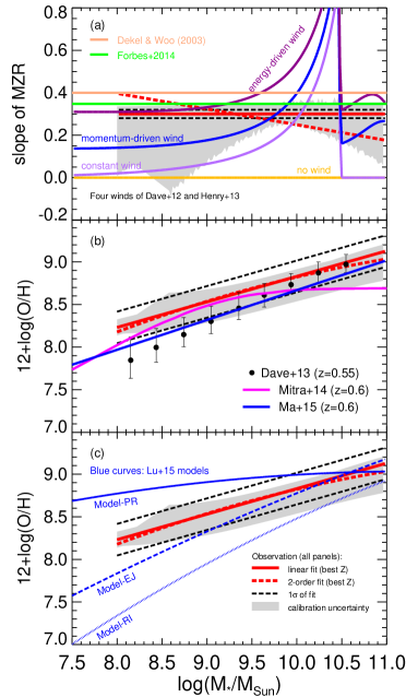
Figure 8.— Comparisons between our MZR and others from theoretical works. In all panel, red solid and dashed lines are best-fit linear and second-order polynomial functions of the DEEP3+TKRS sample, galaxies in which break their lower–upper branch degeneracy by using [OIII]/[OII] (“upper+lower Z”). The black dashed lines are the 1$\sigma$ range of the best linear fit. The gray shaded area is the calibration uncertainties of different metallicity calibrations (Sec. 6.1). Top (a): Slope of the MZRs. Slopes from theoretical works, as the text shows, are over-plotted against our slopes. The sharp discontinuity of wind models around ${\rm M_{*}}$$=10^{10.5}$${\rm M_{\odot}}$ is due to the fact that $\alpha_{Z}$ term in Equation 4 becomes abruptly independent on ${\rm M_{halo}}$ at ${\rm M_{halo}}$$>10^{12}$${\rm M_{\odot}}$. Middle (b): MZRs from Davé et al. (2013); Mitra et al. (2015); Ma et al. (2016) are compared with our MZRs. The symbols with error bars show the 16th, 50th, and 84th percentiles of the data of Davé et al. (2013). Bottom (c): Model MZRs of Lu et al. (2015a) are compared with our MZRs. Blue solid, dashed, and dotted lines are for models with preventative feedback (PR), ejective feedback (EJ), and ejective feedback plus gas reincorporation (RI), respectively.

6.2.3 Equilibrium Model with Monte Carlo Markov Chain (MCMC): Mitra et al. (2015)

Mitra et al. (2015) investigate how well a simple equilibrium model can match observations of key galaxy scaling relations from $z=2$ to $z=0$. The metallicity formula in their paper is similar to our Equation 4:

$$Z=\frac{y}{1+\eta}(1+\frac{\dot{M}_{recyc}}{\zeta\dot{M}_{grav}}),$$ (13)

where $\dot{M}_{recyc}$ is the rate of recycling ejected gases, $\dot{M}_{grav}$ the gas accretion rate (Dekel et al., 2009), and $\zeta$ the preventative feedback parameters. The key baryon cycling parameters are $\eta$, $\zeta$, and $t_{rec}$ (gas recycling timescale). They determine the free parameters by fitting the model to observed scaling relations: ${\rm M_{halo}}$–${\rm M_{*}}$  SFR–${\rm M_{*}}$, and MZR via MCMC. Because MZR is the scaling relation of interest in our paper, we use their best-fit model that only uses ${\rm M_{halo}}$–${\rm M_{*}}$ and SFR–${\rm M_{*}}$ to constrain free parameters. Each parameter is a function of ${\rm M_{halo}}$ and redshift. Their best-fit MZR at $z=0.6$ is shown in Panel (b) of Figure 8, with a yield $y=0.0126$ taken from Asplund et al. (2009).

In the ${\rm M_{*}}$ range of $10^{8.5}$${\rm M_{\odot}}$$<$${\rm M_{*}}$$<10^{9.5}$${\rm M_{\odot}}$, their best-fit MZR matches the normalization of our MZR. But their model underestimates metallicity both very low-mass and massive ends.

At ${\rm M_{*}}$$<10^{8.5}$${\rm M_{\odot}}$, the slope of their MZR is about $\beta_{MZR}\sim 0.5$, steeper than our slope (0.30$\pm$0.02). This is because their best-fit $\gamma$ in our Equation 8 (called $\eta_{3}$ in their paper) is 1.16, much larger than both the momentum-driven and energy-driven wind. According to our discussion above, at $x_{h}\ll 12$, $\beta_{MZR}\sim\gamma\Upsilon$. Given $\Upsilon\sim 0.5$ and $\gamma=1.16$, their $\beta_{MZR}\sim 0.6$. The large $\gamma$ means the mass loading factor at the low-mass end is so large that lots of metals are ejected out of halos, resulting in low gas-phase metallicities.

At ${\rm M_{*}}$$>10^{9.5}$${\rm M_{\odot}}$, their MZR becomes flat ($\beta_{MZR}\sim 0$). Although the “saturation” of metallicity has been reported in the literature (e.g., Zahid et al., 2013, 2014), it usually happens at a much higher ${\rm M_{*}}$ (${\rm M_{*}}$$>10^{10.5}$${\rm M_{\odot}}$). As we discuss above, at ${\rm M_{*}}$$>10^{9.5}$${\rm M_{\odot}}$, metallicity and $\beta_{MZR}$ become more dominated by the gas recycling term. A key parameter in this term is $\zeta$, the preventative feedback parameter. In D12 and Mitra et al. (2015), $\zeta$ is contributed by four sources: photo-ionization, winds, gravitational heating due to structure formation, and quenching of star formation. At $10^{9.5}$${\rm M_{\odot}}$$<$${\rm M_{*}}$$<10^{10.5}$${\rm M_{\odot}}$, the gravitational heating is the dominant contribution. Mitra et al. (2015) uses the formula from the hydrodynamic simulations of Faucher-Giguère et al. (2011), which do not include metal-line cooling. If the metal-line cooling is considered, $\zeta$ would decrease because the heating efficiency becomes lower, which would result in a higher metallicity. We suspect that this could be one reason why the model of Mitra et al. (2015) has lower metallicity than our results at ${\rm M_{*}}$$>10^{9.5}$${\rm M_{\odot}}$.

6.2.4 Hydrodynamic Simulations with Hybrid Winds: Davé et al. (2013)

Motivated by analytic models (Murray et al., 2005, 2010) and hydrodynamic simulations (Hopkins et al., 2012) of outflows from interstellar medium, Davé et al. (2013) use a hybrid wind model in their cosmological hydrodynamic simulations: in dwarf galaxies, the energy from SNe plays a dominant role in driving outflows, while in larger systems, the momentum flux from young stars and/or SNe is the dominant driver. As a result, the outflow scalings switch from momentum-driven at high masses to energy-driven at low masses. The transition occurs at galaxy velocity dispersion $\sigma=75kms^{-1}$ (roughly ${\rm M_{*}}$$\sim 10^{9.5}$${\rm M_{\odot}}$). We show the 16th, 50th, and 84th percentiles of the metallicities of different runs of their simulations in Panel (b) of Figure 8.

Interestingly, the MZR of Davé et al. (2013) matches our MZR very well at ${\rm M_{*}}$$>10^{9.5}$${\rm M_{\odot}}$, but it gradually deviates from ours below ${\rm M_{*}}$$=10^{9.5}$${\rm M_{\odot}}$. This seems inconsistent with our previous discussion, where we show that the energy-driven wind in equilibrium models matches the low-mass end slope of our MZR very well. Similar deviation has been found when Davé et al. (2013) compare their MZR to that at $z=0$ from SDSS (Tremonti et al., 2004), i.e., good agreement at the massive end, but with a steeper-than-observed slope at the low-mass end. A possible reason for the deviation from the energy-driven wind in equilibrium model is that low-mass galaxies in the simulations are not in equilibrium, i.e., $dM_{gas}/dt\neq 0$. Low-mass galaxies grow quite rapidly. Even with the energy-driven wind, the mass-loading factor is not large enough to expel enough gas mass to maintain an “equilibrium”. At decreasing halo (or stellar) mass, the gas reservoir becomes increasingly large relative to what it would be in equilibrium. This makes the slope of the MZR steeper than what is expected from the equilibrium model. Another reason could be the accuracy of the ISM physics adopted in the simulations. Limited by the numerical resolution, most of the cosmological hydrodynamic simulations adopt an approximate (or “sub-grid”) model of ISM physics, star formation, stellar feedback, and galactic winds. In these simulations, in order to prevent low-mass galaxies from forming too many stars, strong outflows are usually required, which would also remove metals from the ISM.

6.2.5 Cosmological Zoom-in Simulations: Ma et al. (2016)

To improve the understanding of the physics of star formation and feedback, Ma et al. (2016) study the redshift evolution of the MZR using the high-resolution cosmological zoom-in simulation FIRE (Hopkins et al., 2014). The resolution (softening factor) of FIRE is 1–10 pc, three orders of magnitude smaller than that of Davé et al. (2013) ($\sim$1 kpc). Such a high resolution allows a realistic characterization of the physics of multi-phase ISM, star formation, feedback, and galactic winds. FIRE includes prescriptions for a few feedback mechanisms: (1) momentum flux from radiative pressure; (2) energy and momentum from SN and stellar winds, and (3) photoionization and photo-electric heating. Ma et al. (2016) include 22 runs of galaxies with various star formation and merger histories.

The slope of the best-fit MZR of FIRE at $z=0.6$ (blue dashed lines in Panel (b) of Figure 8, $\beta_{MZR}=0.35$) shows good agreement with that of our MZR ($\beta_{MZR}=0.30\pm 0.02$). The normalization of their MZR, however, is lower than ours by 0.3 dex. This systematic deviation could be physical or due to their recipe of calculating the effective metal yield, which, as previously discussed, would lead to a 2x uncertainty. Even with this uncertainty, their MZR matches the 1$\sigma$ confidence level of our best-fit MZR (black dashed lines), indicating a statistical agreement.

As stated in Ma et al. (2016), the FIRE galaxies at ${\rm M_{*}}$$>10^{7}$${\rm M_{\odot}}$are able to retain most of the metals they produced in the halos. Massive galaxies (${\rm M_{*}}$$>10^{10}$${\rm M_{\odot}}$) are even able to keep almost all of their metals. This explains why they do not have a “saturation” of metallicity at the massive end. They also find that outflows at outer radii of dark matter halos are much less metal-enriched than those at inner radii, suggesting a high efficiency of metal recycling.

6.2.6 Preventative Feedback (Lu et al., 2015a)

In many semi-analytic models and simulations, there is a tension between suppressing star formation and retaining enough metals in low-mass galaxies. One way to solve it is to use preventative feedback. In contrast to ejective scenarios where the effect of feedback is to remove gas from a galaxy to the intergalactic medium, the preventive scenario assumes some early feedback to change the thermal state of the intergalactic medium around dark matter halos so that a fraction of baryons is prevented from collapsing into low-mass halos in the first place. Therefore, in the preventative model, the outflow strength could be much weaker than that in ejective models. The former would result in a higher gas-phase metallicity.

We compare the predicted MZRs of the preventative and ejective models of Lu et al. (2015a). The details of the models are given in Lu et al. (2015b). We first compare their ejective model (Model-EJ in Panel (c) of Figure 8) to our data. The EJ model captures most of the common features of all ejective models in the literature. In fact, the EJ model matches the hybrid-wind numerical simulations of Davé et al. (2013) very well. Both of them match our MZR at ${\rm M_{*}}$$>10^{9.5}$${\rm M_{\odot}}$, but deviate from our MZR below ${\rm M_{*}}$$=10^{9.5}$${\rm M_{\odot}}$ with a steeper slope. This again demonstrates the common issue of underpredicting metallicity for low-mass galaxies in most of the ejective models.

The second model (Model-RI) of Lu et al. (2015a) predicts a much steeper MZR and significantly underpredicts the average metallicity of low-mass galaxies. This model, as an extension of the ejective model, allows the ejected gas mass to reincorporate into the halo hot gas after a period of time. The reincorporated gas would decrease the gas-phase metallicity. Although the MZR slope of this model is much steeper than our data, it is interesting to see that the predicted metallicity is broadly consistent with those lower-branch galaxies in our sample at $10^{8}$${\rm M_{\odot}}$$<$${\rm M_{*}}$$<10^{9}$${\rm M_{\odot}}$ (Panel (a) of Figure 5). This suggests that those very metal-poor galaxies may have experienced significant re-infallings of their ejected gases. Future work, including robust measurement of the metal-poor galaxies and more accurate modeling, is required to investigate the formation of very metal-poor galaxies.

On the other hand, the preventative model (Model-PR in the same panel) overpredicts the metallicity of low-mass galaxies. Because the main mechanism responsible for keeping baryon mass low in low-mass galaxies is to prevent baryons from collapsing into their host halos, outflow in this model is moderate. Therefore, galaxies in this model retain a larger fraction of metals. The model predicts a rather flat MZR at $z=0.6$, with the metallicity of low-mass (${\rm M_{*}}$$\sim 10^{8}$${\rm M_{\odot}}$) galaxies higher than our data by 0.6 dex.

This result suggests that a pure preventative model cannot explain the MZR at $z=0.6$. Comparing the model predictions with our observational result, we find that the observed MZR sits between the predictions of the Model-EJ and the Model-PR, suggesting that both ejection and prevention work together in low-mass galaxies. Other observations also show evidence of strong outflows (e.g., Rubin et al., 2014), indicating that ejection works at some level, but the effect of outflow in removing hydrogen mass and metal mass is yet to be measured quantitatively. Lu et al. (2015a) also shows that the pure preventative feedback model is able to match the MZR of $z=0$ SDSS galaxies, but overestimates metallicity for $z=2$ galaxies. Therefore, the importance of preventative feedback may also evolve with redshift.

Last but not least, we point out that the predictions made in Lu et al. (2015a) should be considered as upper limits for each scenario. The authors assumed that the metallicity of outflow is the same as the gas-phase metallicity of a galaxy. If the outflow material is more metal enriched relative to the ISM because outflow is driven by SNe, which are the sources of metals, the predicted MZR would decrease.

6.3. Summary of Model Comparisons Using Slope and Normalization

In this section, we compare our MZR at $0.5\leq z\leq 0.7$ to a variety of theoretical works, from simple scaling relation to state-of-the-art numerical simulations. Here we summarize the comparisons of using the slope and normalization of the MZR.

1. Slope. Models (Dekel & Woo, 2003; Forbes et al., 2014b, and D12) incorporating SN energy-driven wind (with mass loading factor $\eta\propto M_{halo}^{(-2/3)}$) provide good agreement with the slope of the MZR of low-mass (${\rm M_{*}}$$<10^{9.5}$${\rm M_{\odot}}$) galaxies. For massive galaxies, gas recycling (the $\alpha_{Z}$ term or its analogs) plays an important role, but the characterization of $\alpha_{Z}$ is uncertain for model comparison. The latest high-resolution simulation FIRE (Hopkins et al., 2014; Ma et al., 2016), which has the ISM physics more accurately characterized thanks to its high resolution, produces a slope in good agreement with ours across the whole ${\rm M_{*}}$ range in our paper.

2. Normalization. With the uncertainty of metal yield $y$ in mind, we find that the hybrid-wind simulation of Davé et al. (2013) and the ejective model of Lu et al. (2015a) match the normalization of our MZR at the massive end. These models, together with Mitra et al. (2015), underestimate the metallicity of low-mass galaxies. One possible solution is to mix preventative (Lu et al., 2015b, a) and ejective feedback for low-mass galaxies.

3. Uncertainties. Our model comparisons are subjected to uncertainties from both observational and theoretical sides. The largest uncertainty of observations is the calibration uncertainty, namely the uncertainty of mapping emission line ratios to metallicities. Two major uncertainties of theoretical models are the metal yield, which can be strongly modulated by the metal enrichment of the outflow material relative to the ISM, and the gas recycling term for massive galaxies.

6.4. Using Slope of the MZR to Link to Dark Matter Halos

The observed slope of the MZR could also reveal new insights in the connection between the luminous (baryonic) and dark (dark matter halo) sides of galaxy formation. This connection can be established through simple analytic models, which usually contain much less parameters than semi-analytic models and even hydrodynamical simulations. Some of these parameters are hard to constrain, as discussed in previous sub-sections. Here, we use the model in Lilly et al. (2013) to demonstrate the efficiency of such analytic models.

The model of Lilly et al. (2013) connects three different aspects of galaxy formation and evolution: (1) evolution of SSFR relative to the growth of dark matter halos, (2) gas-phase metallicities of galaxies, and (3) ${\rm M_{*}}$–${\rm M_{halo}}$ relation. In the model, the formation of stars is instantaneously regulated by the mass of gas in a varying reservoir. The gas in the reservoir is controlled by gas inflow into galaxy and outflow expelled from galaxy, the latter of which is in turn scaled with the SFR.

In the model, gas-phase metallicity is linked to dark matter halos through $f_{gas}$, the ratio of the reduced SFR (i.e., SFR with only long-lived stars counted) to the gas infall rate. Assuming the metallicity of inflow is negligible, we have $Z=f_{gas}y$, where $y$ is the yield. $f_{gas}$ is proportional to the ${\rm M_{*}}$–${\rm M_{halo}}$ relation: $f_{gas}\propto{\rm M_{*}}/{\rm M_{halo}}$. Therefore, the slope of the MZR ($Z\propto{\rm M_{*}}^{\beta_{MZR}}$) and the ${\rm M_{halo}}$–${\rm M_{*}}$ relation (${\rm M_{halo}}\propto{\rm M_{*}}^{\Upsilon}$) has a relation (which is a rearrangement of Equations (32) and (34) of Lilly et al. (2013)):

$$\Upsilon=1-\beta_{MZR},$$ (14)

where $\Upsilon$ has the same definition as that used in Equation 11 and 12.

In Section 6.2.2, we simply take $\Upsilon\sim 0.5$ from Moster et al. (2010) to predict model MZR slopes. Here, we explore the link between the MZR and dark matter halos in the other way: starting from our observed $\beta_{MZR}$ and using it to constrain the ${\rm M_{*}}$–${\rm M_{halo}}$ relation. Using Equation 14, our observed $\beta_{MZR}$=0.30 yields $\Upsilon$=0.70. This value is larger than that of Moster et al. (2010) and hence implies a flatter (${\rm M_{*}}$/${\rm M_{halo}}$)–${\rm M_{halo}}$ relation than that in Moster et al. (2010). It is, however, interesting to note that at ${\rm M_{halo}}$$<10^{11}$${\rm M_{\odot}}$, the slope of the (${\rm M_{*}}$/${\rm M_{halo}}$)–${\rm M_{halo}}$ relation in Behroozi et al. (2013) is indeed flatter than that in Moster et al. (2010) (see Figure 14 in Behroozi et al. (2013)) and quite similar to what inferred from our $\Upsilon$=0.7. Our example here simply aims to highlight the power of using $\beta_{MZR}$ to constrain the physics of dark matter halos. Future investigations are needed to better determine the slope of the (${\rm M_{*}}$/${\rm M_{halo}}$)–${\rm M_{halo}}$ relation at the very low-mass end.

6.5. Using Scatter of the MZR to Understand the Formation of Low-mass Galaxies

The scatter of the MZR is crucial to understand the origin of the MZR. Relative to the slope and normalization, the scatter of the MZR is barely affected by the calibration uncertainty (e.g., Zahid et al., 2012). Therefore, theoretical work on modeling the scatter may provide important clues to understanding galaxy formation. Here, we use the statistical equilibrium model of Forbes et al. (2014b) to demonstrate how to use the scatter to explore the stochastic nature of the formation of low-mass galaxies.

Although the equilibrium models with energy-driven winds provide a good explanation of the slope of the MZR at the low-mass end, its explicit assumption $dM_{gas}/dt=0$ may not be true for all galaxies. For example, Feldmann (2013) and Forbes et al. (2014a) point out that many galaxies are out of the equilibrium with $dM_{gas}/dt<0$. On the other hand, in semi-analytic models (e.g., Lu et al., 2014), low-mass galaxies always increase their gas mass rapidly, namely, $dM_{gas}/dt>0$. Moreover, assuming $dM_{gas}/dt=0$ for all galaxies only allows one to derive the first-order scaling relations; it cannot shed light on the origin of the scatter of the scaling relations.

Forbes et al. (2014b) present a simple model to understand the origin of the scatter in star formation and metallicity of galaxies at a fixed mass. This model relaxes the key assumption of equilibrium models, namely that the rate at which baryons enter the gas reservoir varies slowly. Galaxies in this model have been fed by some stochastic accretion process long enough that the full joint distribution of all galaxy properties has become time invariant. This model can be referred to as a statistical equilibrium model because individual galaxies are not in equilibrium, but the population is. The scatter of scaling relations arises from the intrinsic scatter in the accretion rate and also depends on the time-scale on which the accretion varies compared to the time-scale on which the galaxy loses gas mass.

Forbes et al. (2014b) use $\gamma=2/3$ (see our Equation 8) for the mass loading factor, consistent with energy-driven winds, and they do not include any wind recycling. Given our discussions in Section 6.2.2, not surprisingly, their MZR slope ($\beta_{MZR}=0.348$, the light green line in Panel (a) of Figure 8) matches that of the energy-driven wind ($\beta_{MZR}=0.33$, the magenta line). Their slope agrees with our slope ($0.30\pm 0.02$) for all ${\rm M_{*}}$ ranges within 3$\sigma$ level. These results again suggest the importance of SN feedback on shaping the MZR.

More interesting is to compare the scatter of the MZR in the models of Forbes et al. (2014b) to our data (Panel (b) of Figure 7). Forbes et al. (2014b) do not tune their models to obtain a set of “best-fit” parameters. Instead, they only use two sets of parameters: initial guess and improved guess. The difference between the two sets of parameters allows us to explore the processes responsible for the origin of the scatter of the MZR. The key parameters that govern the scatter of the MZR in their model are (1) the scatter of baryonic accretion rate ($\sigma_{\dot{M}}$) and (2) the scatter of ${\rm M_{*}}$–${\rm M_{halo}}$ relation ($\sigma_{SHMR}$).

The parameters in the initial guess are taken from N-body simulations of Neistein & Dekel (2008) and Neistein et al. (2010). The initial guess yields an MZR scatter of 0.16 (solid gray line in Panel (b) of Figure 7), which matches our scatter around ${\rm M_{*}}$$=10^{9}$${\rm M_{\odot}}$. To produce a scatter smaller than the observed scatter of the local MZR to approach the intrinsic scatter, Forbes et al. (2014b) adjust their key parameters by reducing $\sigma_{\dot{M}}$ and $\sigma_{SHMR}$ by half. The improved guess yields an MZR scatter of 0.09 (dotted gray line in Panel (b) of Figure 7), now matching our MZR scatter of massive galaxies.

The adjustment of the parameters in Forbes et al. (2014b) has an important implication on the origin of the MZR scatter: to increase the MZR scatter, one can increase $\sigma_{\dot{M}}$ and/or $\sigma_{SHMR}$. Galaxies out of (statistical) equilibrium ($dM_{gas}/dt>0$) could also increase the MZR scatter, as argued by Davé et al. (2011b) and Zahid et al. (2012) that the MZR scatter would be large if the timescales for galaxies to equilibrate is long (namely, gas dilution time scale is long compared to the dynamical time scale of galaxies).

Forbes et al. (2014b) predict a constant MZR scatter over the whole ${\rm M_{*}}$ range in both the initial and improved guesses, but our observed scatter increases as ${\rm M_{*}}$ decreases. The difference stems from the assumption in Forbes et al. (2014b) that both $\sigma_{\dot{M}}$ and $\sigma_{SHMR}$ are mass independent. In fact, many current abundance matching methods use a constant $\sigma_{SHMR}$ in their models (e.g., Moster et al., 2010; Behroozi et al., 2013). There is some evidence of a mass-independent $\sigma_{SHMR}$ for massive galaxies with ${\rm M_{*}}$$>10^{10.2}$${\rm M_{\odot}}$ (Trujillo-Gomez et al., 2011; Reddick et al., 2013), but $\sigma_{SHMR}$ of low-mass galaxies has not been well constrained.

The hybrid-wind simulations of Davé et al. (2013) also predict an increasing scatter toward the low-mass end at $z=0.55$ (the solid gray line in Panel (b) of Figure 7). Their scatter matches ours very well for ${\rm M_{*}}$$>10^{9}$${\rm M_{\odot}}$ galaxies. Below ${\rm M_{*}}$$=10^{9}$${\rm M_{\odot}}$, their scatter becomes smaller than ours. In Davé et al. (2013), since the baryonic accretion rate is well set by N-body simulation and their galaxies are probably already out of equilibrium (see Section 6.2.4), one possible explanation of their smaller-than-observed scatter below ${\rm M_{*}}$$=10^{9}$${\rm M_{\odot}}$ is that their $\sigma_{SHMR}$ is smaller than it should be. An additional piece of evidence of an underestimated $\sigma_{SHMR}$ of Davé et al. (2013) is their tighter-than-observed SFR–${\rm M_{*}}$ relation. In the data of Davé et al. (2013), there are almost no galaxies with SFR$>1M_{\odot}/yr$ at ${\rm M_{*}}$$<10^{9}$${\rm M_{\odot}}$. In contrast, our sample contains such galaxies (see Figure 1).

The lack of redshift evolution of the scatter of the MZR is also intriguing. As shown by Panel (b) of Figure 7, our scatter at $z\sim 0.7$ is consistent with that of Tremonti et al. (2004) at $z\sim 0$. This result of no redshift evolution implies that all the factors that could alter the scatter of the MZR should remain unchanged from $z\sim 0.7$ to $z\sim 0$. Among them, $\sigma_{\dot{M}}$ is particularly interesting. Our results suggest that, although the cosmic gas accretion rate decreases by a factor of three during this period (e.g., Dekel et al., 2009), the scatter of the accretion rate remains unchanged from $z\sim 0.7$ to $z\sim 0$. Future theoretical studies on the redshift evolution of the scatter of baryonic accretion rate is important to understand the origin of the scatter of the MZR.

7. Conclusions

We study the MZR and its scatter at $0.5\leq z\leq 0.7$ by using 1381 field galaxies collected from previous deep spectroscopic surveys. Our sample is fairly representative of normal star-forming galaxies at the redshift, in terms of SSFR and color at a given ${\rm M_{*}}$. Moreover, the sample contains 237 galaxies with ${\rm M_{*}}$$<10^{9}$${\rm M_{\odot}}$, comprising currently the largest sample in this mass regime ($\sim$10 times larger than previous ones) beyond the the local universe, which enables an unprecedentedly strong constraint on the MZR and its scatter in the low-mass regime.

We find a power-law MZR with a slope (in logarithmic space) of 0.30$\pm$0.02 at $10^{8}$${\rm M_{\odot}}$$<$${\rm M_{*}}$$<10^{11}$${\rm M_{\odot}}$. Our MZR shows agreement with other MZRs at similar redshifts in the literature at ${\rm M_{*}}$$>10^{9}$${\rm M_{\odot}}$. The slope of our MZR below ${\rm M_{*}}$$\sim 10^{9}$${\rm M_{\odot}}$ is flatter than the extrapolation of other MZRs. The SFR dependence of the MZR in our sample is weaker than that in the local universe. More tests are needed to investigate the existence of the fundamental metallicity relation beyond the local universe.

We compare our MZR to several theoretical models, including simple scaling relations, semi-analytic models, and state-of-the-art numerical simulations. We find that models incorporating SN energy-driven winds (with mass loading factor $\eta\propto M_{halo}^{(-2/3)}$) provide good agreement with the slope of the MZR of galaxies with ${\rm M_{*}}$$<10^{9.5}$${\rm M_{\odot}}$.

With the 10-fold gain in sample size, we present the first measurement of the scatter of the MZR down to ${\rm M_{*}}$$=10^{8}$${\rm M_{\odot}}$ at $0.5\leq z\leq 0.7$. The scatter increases as ${\rm M_{*}}$ decreases, from 0.1 dex at ${\rm M_{*}}$$\sim 10^{10}$${\rm M_{\odot}}$ to 0.3 dex at ${\rm M_{*}}$$\sim 10^{8}$${\rm M_{\odot}}$. The scatter of the MZR shows no evolution from $z\sim 0.7$ to $z\sim 0$.

Relative to the slope and normalization of the MZR, which are subjected to both observational and theoretical uncertainties, the scatter of the MZR is the least affected by observational uncertainties and thus can be used as an important diagnostic of the stochastic formation history of low-mass galaxies. According to a simple statistical equilibrium model, the large scatter in low-mass galaxies implies that either $\sigma_{\dot{M}}$ or $\sigma_{SHMR}$ increases as ${\rm M_{*}}$ decreases. The lack of the redshift evolution of the scatter implies that both $\sigma_{\dot{M}}$ and $\sigma_{SHMR}$ remain unchanged from $z=0.7$ to $z=0$.

We thank the anonymous referee for constructive comments that improve this article. We thank Aldo Rodriguez-Puebla for useful discussions. Several authors from UCSC acknowledge support from NSF grant AST-0808133. Support for Program HST-GO-12060 and HST-AR-13891 were provided by NASA through a grant from the Space Telescope Science Institute, which is operated by the Association of Universities for Research in Astronomy, Incorporated, under NASA contract NAS 5-26555. MR also acknowledges support from an appointment to the NASA Postdoctoral Program at Goddard Space Flight Center. JF is supported by HST-AR-13909. JRT acknowledges support from NASA through Hubble Fellowship grant #51330 awarded by the Space Telescope Science Institute. AD is supported by ISF grant 24/12, by the I-CORE Program of the PBC ISF grant 1829/12, and by NSF grant AST-1405962. PGPG acknowledges support from Spanish MINECO grant AYA2012-31277.

Facilities: Keck (DEIMOS)

Appendix A A. Possible Selection and Measurement Effects on Our MZR

Figure 9.— Selection and measurement effects on our MZR measurement. In all panels, red circles with error bars are the median and 16th and 84th percentiles of the DEEP3+TKRS “upper+lower Z” MZR with ${\rm S/N_{[OIII]andH\beta}}>$3 and H$\beta$ EW correction of 1 Å (the same as that in Panel (a) of Figure 5). Left: S/N cut effect. Blue triangles and green squares show the re-calculated MZRs with ${\rm S/N_{[OIII]andH\beta}}>$8 and 5, respectively. Middle: Sample bias effect. Blue squares and error bars show the MZR of re-sampling our DEEP3+TKRS sample to match the SSFR distribution at a given ${\rm M_{*}}$ of our parent samples. This panel tests the effect of our final sample being biased toward slightly high-SSFR galaxies (see Figure 1). Right: H$\beta$ EW correction effect. Blue squares and error bars show the MZR calculated with H$\beta$ EW correction factor of 3 Å.

Here we discuss three selection and measurement effects that may have impacts on our MZR measurement: (1) S/N cuts on [OIII] and H$\beta$, (2) our sample bias toward higher-SSFR galaxies at ${\rm M_{*}}$$<10^{9.5}$${\rm M_{\odot}}$, and (3) our choice of an H$\beta$ absorption correction factor of EW = 1 Å. We use both the DEEP3+TKRS “upper+lower Z” MZR and the [OIII]/[OII]-derived MZR as our fiducial MZR for the tests. The test results do not change with the choice of the fiducial MZR. For simplicity, we only show the results of the “upper+lower Z” MZR in Figure 9. We conclude that none of the above effects would significantly change the slope and scatter of our MZR.

To investigate the effect of the S/N cuts of emission lines, we re-calculate the MZR with higher S/N cuts, namely ${\rm S/N_{[OIII],H\beta}}>$5 and 8. The new MZRs in the left panel of Figure 9 show that neither cut significantly changes our fiducial results with S/N$>$3. On average, the deviation between the new (blue and green) and the fiducial (red) MZRs is about 0.05 dex. The only large deviation is found at $10^{8}$${\rm M_{\odot}}$$<$${\rm M_{*}}$$<10^{8.5}$${\rm M_{\odot}}$ with S/N$>$8, but the error bars in this mass regime are also the largest. This result is consistent with Foster et al. (2012), who also found that varying the selection criteria of S/N cut or magnitude cut does not significantly alter the MZR for a given calibration. Therefore, we conclude that the S/N cut only induces minor effects on our MZR.

We also investigate the effect of our sample bias on the MZR. As shown in Figure 1, our sample is biased toward high-SSFR galaxies at ${\rm M_{*}}$$<10^{9.5}$${\rm M_{\odot}}$. To derive the MZR for a mass-complete sample, we assign an [OIII]/H$\beta$ value to each star-forming galaxy in our parent samples (CANDELS GOODS-N and IRAC EGS, shown by contours and small black dots in Figure 1). The assigned value is equal to the line ratio of its closest galaxy in the (${\rm M_{*}}$, SSFR) space in our final sample (red symbols in Figure 1). The assumption here is that the [OIII]/H$\beta$ value is determined by its ${\rm M_{*}}$ and SSFR. This assignment is feasible because our selected sample, although biased, actually covers the whole star-forming main sequence. We then re-calculate the MZR for the whole parent sample with the assigned line ratios.

The result (middle panel of Figure 9) shows that the bias in SSFR induces almost no effect on the MZR. This is consistent with our results that the MZR dependence on SSFR is weak in our sample in Section 4.3, where the most obvious (but still weak) signal of SSFR dependence of metallicity is found at $10^{8.5}$${\rm M_{\odot}}$$<$${\rm M_{*}}$$<10^{9.5}$${\rm M_{\odot}}$ (see Figure 6). Therefore, we conclude that our sample is representative of star-forming galaxies for deriving the MZR and its scatter between $10^{8}$${\rm M_{\odot}}$ and $10^{11}$${\rm M_{\odot}}$.

We also test the effect of EW correction for H$\beta$ absorption. We assume a correction factor of 1 Å for our galaxies. Some authors, however, found a higher correction factor (for example, 3 Å in Lilly et al. (2003). We re-calculate the MZR using a correction factor of EW=3Å. The result (right panel of Figure 9) shows that the metallicity of galaxies with $10^{8.5}$${\rm M_{\odot}}$$<$${\rm M_{*}}$$<10^{10.5}$${\rm M_{\odot}}$ is increased by $\sim$0.1 dex. What’s important is that although the increase changes the normalization of the MZR, it does not significantly change its slope or scatter. We emphasize that we use the correction of EW=1 Å as our fiducial results because it is drawn from previous observations with similar spectral resolution as ours. As discussed in Zahid et al. (2011), the EW correction factor depends on the spectral resolution. Lower resolution requires larger correction factors because emission lines are spread into larger wavelength regions. Also, comparison with previous MZRs (Panel (d) of Figure 5) also suggests that using EW=1 Å yields a better agreement with previous results in the literature.

Appendix B B. Effect of AGN Removal

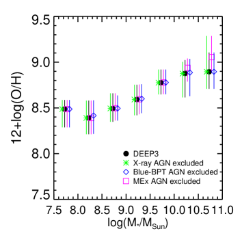
Figure 10.— Effect of AGN removal on the MZR measurement. For simplicity, all galaxies are assumed to be in the upper branch, and no conversion uncertainty is included. Large black circles with error bars show DEEP3+TKRS galaxies without any AGN removal. MZRs with different AGN removal methods are shown by different symbols as indicated by the labels. The MEx method (purple squares) is the fiducial method used in our paper.

As discussed in Section 4.2, AGN removal affects the slope of MZR at the massive end. In this paper, we use the MEx method of Juneau et al. (2011) to exclude AGN contamination. Juneau et al. (2011) used the DEEP2 and TKRS spectra (the same data as used by this paper) to calibrate their method to achieve a balance between efficiency and contamination. Also, the MEx method is shown remaining effective up to $z=1.5$ (Trump et al., 2013). Therefore, we believe that the MEx method is the most suitable one for our study. In Figure 10, we re-calculate the MZR by using other AGN removal methods and compare the results to our fiducial MZR of using the MEx method.

X-ray is the most reliable way to identify AGNs, but it is not complete, due to a significant (up to  50%) fraction of Compton-thick AGNs. Therefore, the results of using X-ray selection should only be treated as a lower limit of AGN contamination. As shown in Figure 10, X-ray selection removes fewer high-metallicity (i.e., high [OIII]/H$\beta$) galaxies at ${\rm M_{*}}$$>10^{10}$${\rm M_{\odot}}$than the MEx method does, resulting in an almost flat MZR at this mass regime. The massive-end slope is now more consistent with that of Zahid et al. (2013) because Zahid et al. (2013) also only removed X-ray sources.

AGN removal can also be done with the “Blue BPT” diagram (Lamareille et al., 2004; Lamareille, 2010) which uses [OIII]/H$\beta$ vs. [OII]/H$\beta$ to identify AGNs. Compared to the MEx method, the “Blue BPT” introduces no explicit mass dependence. It, however, requires measurement of dust extinction because [OII]/H$\beta$ is reddening dependent. Lamareille (2010) argues that using EW ratios could alleviate the issue, but this does not fully remove the reddening-dependence because stars and gas have different extinction. Figure 10 shows that the “Blue BPT” removal results in a very similar MZR to the MEx (and X-ray) removal at ${\rm M_{*}}$$<10^{10.5}$${\rm M_{\odot}}$. At higher ${\rm M_{*}}$(where small number statistics hits our sample), the “Blue BPT” result is similar to that of X-ray removal.

Overall, we conclude: (1) X-ray selection provides the most reliable AGN identification, but its identified AGN sample is not complete. Line-ratio diagnostics are needed to exclude Compton-thick AGNs. (2) MEx of Juneau et al. (2011) is defined at $z\sim 0.7$ and hence the most suitable method for our study. (3) “Blue BPT” yield a similar result to X-ray selection. (4) What’s important is that the three methods result in almost same MZR at ${\rm M_{*}}$$<10^{10.5}$${\rm M_{\odot}}$. This is because AGN contamination is very little in low-mass galaxies (Trump et al., 2015). Therefore, our main conclusions on both the slope and scatter of MZR at ${\rm M_{*}}$$<10^{10.5}$${\rm M_{\odot}}$ are unaffected by our AGN removal.

References

- Allende Prieto et al. (2001) Allende Prieto, C., Lambert, D. L., & Asplund, M. 2001, ApJ, 556, L63
- Amorín et al. (2014) Amorín, R., Sommariva, V., Castellano, M., et al. 2014, A&A, 568, L8
- Asplund et al. (2009) Asplund, M., Grevesse, N., Sauval, A. J., & Scott, P. 2009, ARA&A, 47, 481
- Atek et al. (2010) Atek, H., Malkan, M., McCarthy, P., et al. 2010, ApJ, 723, 104
- Balestra et al. (2010) Balestra, I., Mainieri, V., Popesso, P., et al. 2010, A&A, 512, A12
- Barro et al. (2011a) Barro, G., Pérez-González, P. G., Gallego, J., et al. 2011a, ApJS, 193, 13
- Barro et al. (2011b) Barro, G., Pérez-González, P. G., Gallego, J., et al. 2011b, ApJS, 193, 30
- Barro et al. (2013) Barro, G., Faber, S. M., Pérez-González, P. G., et al. 2013, ApJ, 765, 104
- Behroozi et al. (2013) Behroozi, P. S., Wechsler, R. H., & Conroy, C. 2013, ApJ, 770, 57
- Bruzual & Charlot (2003) Bruzual, G., & Charlot, S. 2003, MNRAS, 344, 1000
- Calzetti et al. (2000) Calzetti, D., Armus, L., Bohlin, R. C., et al. 2000, ApJ, 533, 682
- Chabrier (2003) Chabrier, G. 2003, PASP, 115, 763
- Cid Fernandes et al. (2007) Cid Fernandes, R., Asari, N. V., Sodré, L., et al. 2007, MNRAS, 375, L16
- Colbert et al. (2013) Colbert, J. W., Teplitz, H., Atek, H., et al. 2013, ApJ, 779, 34
- Cooper et al. (2011) Cooper, M. C., Aird, J. A., Coil, A. L., et al. 2011, ApJS, 193, 14
- Cooper et al. (2012) Cooper, M. C., Griffith, R. L., Newman, J. A., et al. 2012, MNRAS, 419, 3018
- Cowie & Barger (2008) Cowie, L. L., & Barger, A. J. 2008, ApJ, 686, 72
- Cresci et al. (2012) Cresci, G., Mannucci, F., Sommariva, V., et al. 2012, MNRAS, 421, 262
- Croton et al. (2006) Croton, D. J., Springel, V., White, S. D. M., et al. 2006, MNRAS, 365, 11
- Davé et al. (2011a) Davé, R., Finlator, K., & Oppenheimer, B. D. 2011a, MNRAS, 416, 1354
- Davé et al. (2012) Davé, R., Finlator, K., & Oppenheimer, B. D. 2012, MNRAS, 421, 98
- Davé et al. (2013) Davé, R., Katz, N., Oppenheimer, B. D., Kollmeier, J. A., & Weinberg, D. H. 2013, MNRAS, 434, 2645
- Davé et al. (2011b) Davé, R., Oppenheimer, B. D., & Finlator, K. 2011b, MNRAS, 415, 11
- de los Reyes et al. (2015) de los Reyes, M. A., Ly, C., Lee, J. C., et al. 2015, AJ, 149, 79
- Dekel & Silk (1986) Dekel, A., & Silk, J. 1986, ApJ, 303, 39
- Dekel & Woo (2003) Dekel, A., & Woo, J. 2003, MNRAS, 344, 1131
- Dekel et al. (2009) Dekel, A., Birnboim, Y., Engel, G., et al. 2009, Nature, 457, 451
- Erb et al. (2006) Erb, D. K., Shapley, A. E., Pettini, M., et al. 2006, ApJ, 644, 813
- Faucher-Giguère et al. (2011) Faucher-Giguère, C.-A., Kereš, D., & Ma, C.-P. 2011, MNRAS, 417, 2982
- Feldmann (2013) Feldmann, R. 2013, MNRAS, 433, 1910
- Finlator & Davé (2008) Finlator, K., & Davé, R. 2008, MNRAS, 385, 2181
- Forbes et al. (2014a) Forbes, J. C., Krumholz, M. R., Burkert, A., & Dekel, A. 2014a, MNRAS, 438, 1552
- Forbes et al. (2014b) Forbes, J. C., Krumholz, M. R., Burkert, A., & Dekel, A. 2014b, MNRAS, 443, 168
- Foster et al. (2012) Foster, C., Hopkins, A. M., Gunawardhana, M., et al. 2012, A&A, 547, A79
- Grasshorn Gebhardt et al. (2016) Grasshorn Gebhardt, H. S., Zeimann, G. R., Ciardullo, R., et al. 2016, ApJ, 817, 10
- Grogin et al. (2011) Grogin, N. A., Kocevski, D. D., Faber, S. M., et al. 2011, ApJS, 197, 35
- Guo et al. (2013) Guo, Y., Ferguson, H. C., Giavalisco, M., et al. 2013, ApJS, 207, 24
- Henry et al. (2013a) Henry, A., Martin, C. L., Finlator, K., & Dressler, A. 2013a, ApJ, 769, 148
- Henry et al. (2013b) Henry, A., Scarlata, C., Domínguez, A., et al. 2013b, ApJ, 776, L27
- Hopkins et al. (2014) Hopkins, P. F., Kereš, D., Oñorbe, J., et al. 2014, MNRAS, 445, 581
- Hopkins et al. (2012) Hopkins, P. F., Quataert, E., & Murray, N. 2012, MNRAS, 421, 3522
- Hoyos et al. (2005) Hoyos, C., Koo, D. C., Phillips, A. C., Willmer, C. N. A., & Guhathakurta, P. 2005, ApJ, 635, L21
- Juneau et al. (2011) Juneau, S., Dickinson, M., Alexander, D. M., & Salim, S. 2011, ApJ, 736, 104
- Kennicutt (1998) Kennicutt, Jr., R. C. 1998, ARA&A, 36, 189
- Kewley & Dopita (2002) Kewley, L. J., & Dopita, M. A. 2002, ApJS, 142, 35
- Kewley et al. (2013) Kewley, L. J., Dopita, M. A., Leitherer, C., et al. 2013, ApJ, 774, 100
- Kewley & Ellison (2008) Kewley, L. J., & Ellison, S. L. 2008, ApJ, 681, 1183
- Koekemoer et al. (2011) Koekemoer, A. M., Faber, S. M., Ferguson, H. C., et al. 2011, ApJS, 197, 36
- Kriek et al. (2009) Kriek, M., van Dokkum, P. G., Labbé, I., et al. 2009, ApJ, 700, 221
- Lamareille (2010) Lamareille, F. 2010, A&A, 509, A53
- Lamareille et al. (2004) Lamareille, F., Mouhcine, M., Contini, T., Lewis, I., & Maddox, S. 2004, MNRAS, 350, 396
- Lee et al. (2006) Lee, H., Skillman, E. D., Cannon, J. M., et al. 2006, ApJ, 647, 970
- Lilly et al. (2013) Lilly, S. J., Carollo, C. M., Pipino, A., Renzini, A., & Peng, Y. 2013, ApJ, 772, 119
- Lilly et al. (2003) Lilly, S. J., Carollo, C. M., & Stockton, A. N. 2003, ApJ, 597, 730
- Lu et al. (2015a) Lu, Y., Mo, H. J., & Lu, Z. 2015a, ArXiv e-prints, 1504.02109
- Lu et al. (2015b) Lu, Y., Mo, H. J., & Wechsler, R. H. 2015b, MNRAS, 446, 1907
- Lu et al. (2014) Lu, Y., Wechsler, R. H., Somerville, R. S., et al. 2014, ApJ, 795, 123
- Ly et al. (2014) Ly, C., Malkan, M. A., Nagao, T., et al. 2014, ApJ, 780, 122
- Ly et al. (2015) Ly, C., Rigby, J. R., Cooper, M., & Yan, R. 2015, ApJ, 805, 45
- Ma et al. (2016) Ma, X., Hopkins, P. F., Faucher-Giguère, C.-A., et al. 2016, MNRAS, 456, 2140
- Maier et al. (2014) Maier, C., Lilly, S. J., Ziegler, B. L., et al. 2014, ApJ, 792, 3
- Maier et al. (2015) Maier, C., Ziegler, B. L., Lilly, S. J., et al. 2015, A&A, 577, A14
- Maiolino et al. (2008) Maiolino, R., Nagao, T., Grazian, A., et al. 2008, A&A, 488, 463
- Mannucci et al. (2010) Mannucci, F., Cresci, G., Maiolino, R., Marconi, A., & Gnerucci, A. 2010, MNRAS, 408, 2115
- Mannucci et al. (2011) Mannucci, F., Salvaterra, R., & Campisi, M. A. 2011, MNRAS, 414, 1263
- Mitra et al. (2015) Mitra, S., Davé, R., & Finlator, K. 2015, MNRAS, 452, 1184
- Moster et al. (2010) Moster, B. P., Somerville, R. S., Maulbetsch, C., et al. 2010, ApJ, 710, 903
- Murray et al. (2005) Murray, N., Quataert, E., & Thompson, T. A. 2005, ApJ, 618, 569
- Murray et al. (2010) Murray, N., Quataert, E., & Thompson, T. A. 2010, ApJ, 709, 191
- Nagao et al. (2006) Nagao, T., Maiolino, R., & Marconi, A. 2006, A&A, 459, 85
- Neistein & Dekel (2008) Neistein, E., & Dekel, A. 2008, MNRAS, 383, 615
- Neistein et al. (2010) Neistein, E., Macciò, A. V., & Dekel, A. 2010, MNRAS, 403, 984
- Newman et al. (2013) Newman, J. A., Cooper, M. C., Davis, M., et al. 2013, ApJS, 208, 5
- Oke (1974) Oke, J. B. 1974, ApJS, 27, 21
- Peeples & Shankar (2011) Peeples, M. S., & Shankar, F. 2011, MNRAS, 417, 2962
- Pérez et al. (2016) Pérez, J. M., Hoyos, C., Díaz, Á. I., Koo, D. C., & Willmer, C. N. A. 2016, MNRAS, 455, 3359
- Pérez-Montero et al. (2013) Pérez-Montero, E., Contini, T., Lamareille, F., et al. 2013, A&A, 549, A25
- Reddick et al. (2013) Reddick, R. M., Wechsler, R. H., Tinker, J. L., & Behroozi, P. S. 2013, ApJ, 771, 30
- Rubin et al. (2014) Rubin, K. H. R., Prochaska, J. X., Koo, D. C., et al. 2014, ApJ, 794, 156
- Salim et al. (2015) Salim, S., Lee, J. C., Davé, R., & Dickinson, M. 2015, ApJ, 808, 25
- Sanders et al. (2015) Sanders, R. L., Shapley, A. E., Kriek, M., et al. 2015, ApJ, 799, 138
- Searle & Sargent (1972) Searle, L., & Sargent, W. L. W. 1972, ApJ, 173, 25
- Somerville & Davé (2015) Somerville, R. S., & Davé, R. 2015, ARA&A, 53, 51
- Steidel et al. (2014) Steidel, C. C., Rudie, G. C., Strom, A. L., et al. 2014, ApJ, 795, 165
- Tinsley & Larson (1978) Tinsley, B. M., & Larson, R. B. 1978, ApJ, 221, 554
- Tremonti et al. (2004) Tremonti, C. A., Heckman, T. M., Kauffmann, G., et al. 2004, ApJ, 613, 898
- Trujillo-Gomez et al. (2011) Trujillo-Gomez, S., Klypin, A., Primack, J., & Romanowsky, A. J. 2011, ApJ, 742, 16
- Trump et al. (2013) Trump, J. R., Konidaris, N. P., Barro, G., et al. 2013, ApJ, 763, L6
- Trump et al. (2015) Trump, J. R., Sun, M., Zeimann, G. R., et al. 2015, ApJ, 811, 26
- Wirth et al. (2004) Wirth, G. D., Willmer, C. N. A., Amico, P., et al. 2004, AJ, 127, 3121
- Wuyts et al. (2011) Wuyts, S., Förster Schreiber, N. M., Lutz, D., et al. 2011, ApJ, 738, 106
- Zahid et al. (2012) Zahid, H. J., Bresolin, F., Kewley, L. J., Coil, A. L., & Davé, R. 2012, ApJ, 750, 120
- Zahid et al. (2014) Zahid, H. J., Dima, G. I., Kudritzki, R.-P., et al. 2014, ApJ, 791, 130
- Zahid et al. (2013) Zahid, H. J., Geller, M. J., Kewley, L. J., et al. 2013, ApJ, 771, L19
- Zahid et al. (2011) Zahid, H. J., Kewley, L. J., & Bresolin, F. 2011, ApJ, 730, 137