Persistent currents, deformation and collectivity in the many-boson yrast problem on the circle

Abstract

Properties of the yrast states of a system of $N$ bosons confined to a one-dimensional ring and interacting via contact forces is examined both variationally and by numerical diagonalizations. The latter allow for obtaining numerical correlated many-body wave functions explicitly. The study of correlation functions involving different yrast states indicates that a quantum phase transition previously detected in the properties of the ground state in the case of attractive two-body interactions is an yrast phenomenon involving the onset of ‘deformation’, in the sense given to this term by Bohr and Mottelson in connection with the description of nuclear spectra, including enhanced transition operators and emergence of a shared intrinsic correlation structure. In this case the moment of inertia of the deformed state is essentially the rigid moment of inertia, ‘intrinsic’ states being essentially degenerate.

1 Introduction.

Persistent matter currents in the multiply connected ring geometry have now been experimentally realized and studied many times in connection with ultra cold bosonic gases[1, 2, 3] in order to explore super fluid properties of the underlying many-body system. The most salient feature present in all cases is the ‘quantization of the persistent current with macroscopic values of the angular momentum’ which was dubbed macroscopic isomerism by Bohr and Mottelson more than 50 years ago[4], in connection with the quantization and (meta-)stability of electric currents in superconductors. In the case of the bosonic gases, the relevant ‘macroscopic’ values of the angular momentum $L$ are (in units of $\hbar$) the integer multiples of the number of particles $N$.

Such macroscopic quantization was long ago dealt with, in the Bose gas context, by F. Bloch[5]. This work appeared in the wake of related work on superconductivity[6] and is based on a detailed analysis of the minimum energies involved in imparting given amounts of angular momentum to the system ground state. The analysis was carried out in the context of a simple (one-dimensional) microscopic quantum mechanical model, revived and extended more recently by several authors[7, 8, 9]. In particular, the occurrence of a quantum phase transition was pointed out in [7] in a study of the ground state properties with attractive two-body effective interactions. It was signalled by the ‘solitonic’ breaking of the rotational symmetry in an effective mean field approach, and corroborated by the behavior of the ground state two-body correlation function obtained by diagonalizing the effective Hamiltonian in a Fock subspace with good particle number and total angular momentum.

Symmetries, such as rotational invariance, play a most important role in organizing the dynamical properties of finite quantum many-body systems. However, is also well known that there are many phenomenologically salient features which develop across the cleavage resulting from them. A familiar example of this is the occurrence of rotational spectra in molecules and atomic nuclei which involve subspaces of different angular momenta, even though they are dynamically disjoint as a result of rotational invariance. Such features are currently described in terms of the stability of certain symmetry violating correlation properties, or ‘deformations’[10]. The resulting syndrome is in fact the finite-system counterpart of the spontaneous breaking of symmetries which can occur in extended systems.

In this work we study, as a function of angular momentum, the low energy quantal spectrum of a dilute bosonic gas confined to a quasi one-dimensional toroidal trap, assuming the usual zero-range effective two-body interaction based on the s-wave scattering length. This is done taking advantage of the strictly finite nature of the system and adopting two independent approaches, namely a) using a variational treatment involving product states with possibly broken rotational symmetry while constraining the mean value of the angular momentum per particle and b) by carrying out numerical diagonalization of the Hamiltonian in many-body subspaces of definite particle number and angular momentum, built from the different possible occupations of a restricted set of relevant single-particle states. Both effectively repulsive and attractive two-body interactions are considered. We find in both cases that the qualitative features of the system are at most weakly dependent on the number of particles provided the effective two body interaction strength is scaled with $1/N$ so as to preserve the relative weight of the kinetic (one-body) and the interaction (two-body) dynamical ingredients at fixed trap geometry.

We find that the effect of repulsive effective two-body interactions is essential for providing conditions for macroscopic isomerism (or persistent current meta-stability) in the model[5, 11]. The strengths prevailing in current realistic experimental situations are in fact orders of magnitude larger as compared with threshold values obtained for several lowest values of $L/N$. Attractive two-body effective interactions are found to lead to the onset of a regime in which the excitation energies of the lowest states of each successive value of the total angular momentum correspond to the energies of an essentially rigid rotational band with the rigid moment of inertia. In this way, the quantum phase transition pointed out in ref. [7] appears as an yrast phenomenon associated to the emergence of a correlation structure common to a family of states with different values on the total angular momentum. This is clearly akin to ‘deformation’ as found in connection with rotational spectra in nuclear and molecular physics. We find also that the correlation structure induced by attractive (repulsive) two-body interactions strongly enhances (appreciably reduces) transition matrix elements involving a one body angular momentum exchange operator along the yrast line and so will affect decay rates for processes dependent on such matrix elements. It should be kept in mind, however that observed decay probabilities (as e.g. in [2]) may well involve degrees of freedom beyond those of the present quasi one-dimensional model.

2 Hamiltonian.

The Hamiltonian for scalar bosons in a tight toroidal trap of radius $R$ and cross section $S$ is

$$H=\frac{\hbar^{2}}{2MR^{2}}\int_{0}^{2\pi}d\varphi\psi^{\dagger}(\varphi)l_{z}^{2}\psi(\varphi)+\frac{1}{2}\frac{U_{c}}{RS}\int_{0}^{2\pi}\psi^{\dagger}(\varphi)\psi^{\dagger}(\varphi)\psi(\varphi)\psi(\varphi)d\varphi$$ (1)

where $\psi(\varphi),\psi^{\dagger}(\varphi)$ are the field operators, $l_{z}=-i\frac{\partial}{\partial\varphi}$ is the angular momentum operator in units of $\hbar$ and $U_{c}=4\pi\frac{\hbar^{2}a}{M}$ is the strength of the effective two-body, 3-D contact interaction, $a$ being the scattering length.

Introducing bosonic creation and annihilation operators $b_{m}^{\dagger}$ and $b_{m}$ for atoms in the single particle angular momentum eigenstates

$$\phi_{m}(\varphi)=\frac{1}{\sqrt{2\pi}}e^{im\varphi},\hskip 28.45274pt\int_{0}^{2\pi}d\varphi\phi_{m^{\prime}}^{*}(\varphi)\phi_{m}(\varphi)=\delta_{m^{\prime},m},$$ (2)

and expanding the field operators as

$$\psi(\varphi)=\sum_{m}\phi_{m}(\varphi)b_{m},$$ (3)

the Hamiltonian (1) can be expressed as

$$H = \frac{\hbar^{2}}{2MR^{2}}\sum_{m}m^{2}b_{m}^{\dagger}b_{m}+\frac{\Lambda}{2}\sum_{m_{i}}b_{m_{1}}^{\dagger}b_{m_{2}}^{\dagger}b_{m_{3}}b_{m_{4}}\delta_{m_{1}+m_{2},m_{3}+m_{4}}\equiv$$ (4)

$$\equiv K+V$$

where $\frac{\hbar^{2}}{2MR^{2}}$ and $\Lambda\equiv\frac{U_{c}}{2\pi RS}$ set the kinetic and interaction energy scales.

This second quantized Hamiltonian commutes with the number operator ${\cal{N}}=\sum_{m}b^{\dagger}_{m}b_{m}$. In each of the Fock space sectors characterized by the particle number $N$ (where ${\cal{N}}$ acts as the corresponding multiple of the unit operator), it can be split into ‘center of mass’ and ‘intrinsic’ parts by introducing the total angular momentum operator (in units of $\hbar$) $L_{z}\equiv\sum_{m}m\;b_{m}^{\dagger}b_{m}$, also a constant of motion, and writing its kinetic energy part as

$$K=\frac{\hbar^{2}L_{z}^{2}}{2NMR^{2}}+K_{\rm int}$$

with

$$K_{\rm int}=\frac{\hbar^{2}}{4NMR^{2}}\sum_{m_{1}m_{2}}(m_{1}-m_{2})^{2}b_{m_{1}}^{\dagger}b_{m_{2}}^{\dagger}b_{m_{2}}b_{m_{1}}$$

which can be easily verified to be algebraically equivalent to the kinetic energy term of eq. (4). The center of mass part is clearly just the rigid rotational energy $\frac{\hbar^{2}L_{z}^{2}}{2NMR^{2}}$, which commutes both with the intrinsic part $K_{\rm int}$ of the kinetic energy and with the potential energy term $V$. One has therefore

$$H=K_{\rm CM}+H_{\rm int}\hskip 28.45274pt{\rm with}\hskip 28.45274ptH_{\rm int}=K_{\rm int}+V.$$ (5)

Since the total angular momentum $L_{z}$ is also a constant of motion, the stationary states of $H$ and of $H_{\rm int}$ can be chosen as states with good total angular momentum $L$.

3 The spectrum of $H_{\rm int}$.

Here we briefly review the results of F. Bloch [5] within the specific context of the Hamiltonian (1) or (4). In view of the decomposition (5) of this Hamiltonian, the eigenvalues $E_{L}$ of states with total angular momentum $L$ can in turn be split as

$$E_{L}=\frac{\hbar^{2}L^{2}}{2NMR^{2}}+e_{\rm int}^{(L)}$$ (6)

where the last term is an eigenvalue of the intrinsic Hamiltonian $H_{\rm int}$ also associated with the total angular momentum $L$. The corresponding $N$-particle eigenstate can be expanded in the occupation number base vectors $|\{n_{m}\}_{N,L}\rangle\equiv\prod_{m}\frac{1}{\sqrt{n_{m}!}}\left(b^{\dagger}_{m}\right)^{n_{m}}|0\rangle$, built on single particle states with good angular momentum $m$ and satisfying the conditions $\sum_{m}n_{m}=N$ and $\sum_{m}m\,n_{m}=L$, as

$$|\Psi_{E_{L}^{(j)}}\rangle=\sum_{\{n_{m}\}_{N,L}}C_{\{n_{m}\}_{N,L}}^{(j)}\prod_{m}\frac{1}{\sqrt{n_{m}!}}\left(b^{\dagger}_{m}\right)^{n_{m}}|0\rangle.$$ (7)

Since the intrinsic Hamiltonian $H_{\rm int}$ depends only on relative angular momenta of particle pairs[13], it follows that the vectors obtained from this expansion just by shifting all the single particle angular momenta $m$ by an integer $l$, i.e.

$$|\Psi_{E_{L+lN}^{(j)}}\rangle=\sum_{\{n_{m}\}_{N,L}}C_{\{n_{m}\}_{N,L}}^{(j)}\prod_{m}\frac{1}{\sqrt{n_{m}!}}\left(b^{\dagger}_{(m+l)}\right)^{n_{m}}|0\rangle,$$

will have the same intrinsic energy, while the total angular momentum is shifted by $lN$, so that the center of mass energy is $\frac{\hbar^{2}(L+lN)^{2}}{2NMR^{2}}$. This implies that the spectrum of $H_{\rm int}$ is periodic in $L$ with period $N$. Furthermore, invariance of the spectrum under the replacement of the base vectors $|\{n_{m}\}_{N,L}\rangle$ by $|\{n_{-m}\}_{N,-L}\rangle$ guarantees that the $L$-dependence of the periodic intrinsic spectrum is also reflection symmetric.

Of special relevance here is the set lowest eigen-energies for each value of the total angular momentum (the set of the so called yrast states, or the yrast line[12]). In view of the above properties, the energy eigenvalues on this line will be given as the addition of the set of lowest intrinsic energies for increasing values of the total angular momentum $L$ (which is periodic in $L$ with period $N$) to the the center of mass energy parabola $\frac{\hbar^{2}L^{2}}{2NMR^{2}}$. As argued in ref. [5] (see also ref. [11]), the occurrence of minima along the yrast line at non vanishing values of the total angular momentum signals the existence of meta-stable states with persistent currents in the system when additional couplings allowing for angular momentum and energy exchange between the system and the constraining environment.

4 Characterization of the yrast line I - variational approach.

In view of the general periodicity features just described, it is convenient to write the total angular momentum $L$ (in units of $\hbar$) as $L=N(l+\nu)$, $l$ being the integer part of the ratio $L/N$ and $\nu=0,\frac{1}{N},\frac{2}{N},\dots,\frac{N-1}{N}$. In this way, it is easily ascertained that the intrinsic energies for a system of free bosons in the ring are given by

$$\frac{e_{\rm int}^{(L)}}{N}=\frac{\hbar^{2}}{2MR^{2}}\,\nu(1-\nu),\hskip 28.45274pt\nu=0,\frac{1}{N},\frac{2}{N},\dots,\frac{N-1}{N}$$

They are independent of $l$, consistently with the periodicity of the intrinsic spectrum. One sees moreover i) that the intrinsic yrast energies display cusp minima at the integer values of $L$, and ii) that the only minimum of the yrast line (including the center of mass rotational energy) for the free bosons occurs at $L=0$.

In order to explore variationally the effects of the effective two body interaction on the yrast energies we make use of the family of ‘condensate’ states[8]

$$|\Psi\rangle\equiv\frac{1}{\sqrt{N!}}\left(A^{\dagger}\right)^{N}|0\rangle$$

with

$$A^{\dagger}\equiv c_{l-1}b_{l-1}^{\dagger}+c_{l}b_{l}^{\dagger}+c_{l+1}b_{l+1}^{\dagger}\hskip 14.22636pt{\rm and}\hskip 14.22636pt|c_{l-1}|^{2}+|c_{l}|^{2}+|c_{l+1}|^{2}=1,$$ (8)

so that $[A,A^{\dagger}]=1$. These states are used to obtain approximations to the yrast line energies associated with angular momenta $L=N(l+\nu)$. The approximate energies are given by the value of the energy functional $\langle\Psi|H|\Psi\rangle$ in the state $|\Psi\rangle$ which minimizes this value under the constraint $\langle\Psi|L_{z}|\Psi\rangle=L$, which is expressed in terms of the amplitudes involved in the definition of $A^{\dagger}$ as

$$|c_{l+1}|^{2}-|c_{l-1}|^{2}=\nu.$$ (9)

The constraints (8) and (9) are taken into account by introducing the parameterization

$$c_{l}=e^{i\alpha_{l}}|c_{l}|,\;\,\;\,c_{l+1}=e^{i\alpha_{l+1}}\sqrt{\frac{1+\nu-|c_{l}|^{2}}{2}},\;\,\;\,c_{l-1}=e^{i\alpha_{l-1}}\sqrt{\frac{1-\nu-|c_{l}|^{2}}{2}}$$

in which the variational parameters are $|c_{l}|$ (restricted to the domain $0<|c_{l}|^{2}<1-\nu$) and the phases $\alpha_{l-1}$, $\alpha_{l}$ and $\alpha_{l+1}$. The evaluation of the energy functional is then straightforward. In units of $\frac{\hbar^{2}}{2MR^{2}}$ the energy functional per particle reads

$${\cal{F}}_{l}(|c_{l}|,\Phi,\nu)\equiv\frac{2MR^{2}}{\hbar^{2}}\frac{\langle\Psi|H|\Psi\rangle}{N}=\frac{L^{2}}{N^{2}}+1-\nu^{2}-|c_{l}|^{2}+$$

$$+ g\left(\frac{3}{4}+\frac{|c_{l}|^{2}}{2}-\frac{3}{4}|c_{l}|^{4}-\frac{\nu^{2}}{4}+|c_{l}|^{2}\sqrt{\left(1-|c_{l}|^{2}\right)^{2}-\nu^{2}}\cos\Phi\right)$$

where $\Phi=2\alpha_{l}-\alpha_{l+1}-\alpha_{l-1}$ and $g$ is the dimensionless interaction strength

$$g\equiv(N-1)\frac{2MR^{2}}{\hbar^{2}}\Lambda=(N-1)\frac{4Ra}{S}.$$

Note the $(N-1)$ factor included in this constant. This is done so that, if the number of particles $N$ is increased at fixed $g$, (e.g. by scaling $a$ with $1/(N-1)$ and keeping the geometrical parameters $R$ and $S$ fixed), then the one- and two-body contributions to the energy functional will both scale with $N$[14]. The fact that the energy functional depends on the phases of the variational parameters $c_{j}$ only through the combination $\Phi$ is a consequence of invariance under the transformation $\alpha_{l+k}\rightarrow\alpha_{l+k}+k\phi$, $k=0,\pm 1$, associated with the rotational invariance of $H$, together with invariance under a global phase change $\alpha_{j}\rightarrow\alpha_{j}+\phi$, associated with the global gauge invariance of $H$. Note also that the functional (4) satisfies the Bloch decomposition (6), being of the form

$${\cal{F}}_{l}(|c_{l}|,\Phi,\nu)=\frac{L^{2}}{N^{2}}+{\cal{F}}_{l}^{\rm int}(|c_{l}|,\Phi,\nu),\hskip 28.45274ptL=N(l+\nu).$$ (11)

The last term of (11) is independent of $l$, implying the periodicity ${\cal{F}}_{l}^{\rm int}(|c_{l}|,\Phi,\nu)={\cal{F}}_{0}^{\rm int}(|c_{0}|,\Phi,\nu)$. This allows in particular to restrict further considerations to $l=0$ only in connection with the intrinsic part of the energy functional.

Fig. 1: Chart of the relevant minima of the intrinsic energy functional ${\cal{F}}_{l}^{\rm int}(|\bar{c_{0}}|,\bar{\Phi},\nu)$ in the $|c_{0}|^{2}\times g$ plane for $\nu=0$. The curve at $|c_{0}|^{2}>\frac{3}{7}$, $g<-0.5$ corresponds to absolute minima with $\Phi=0$. It joins the straight line at $|c_{0}|^{2}=1$ which corresponds to ‘infima’ with $\Phi=0,\pi$ for $g>-0.5$. Secondary minima are indicated at $|c_{0}|^{2}=0$, with $\Phi=\pi$ for $g<-2$ and $\Phi=0$ for $g>\frac{2}{3}$, and secondary ‘infima’ occur at $|c_{0}|^{2}=1$ with $\Phi=\pi$ and $g<-0.5$.

The global minima of the intrinsic energy functional are taken as variational approximations to the intrinsic yrast energies, i. e.

$$\left.\begin{array}[]{l}\frac{\partial{\cal{F}}_{0}^{\rm int}}{\partial\Phi}(|\bar{c_{0}}|,\bar{\Phi},\nu)=0\\ \\ \frac{\partial{\cal{F}}_{0}^{\rm int}}{\partial|c_{0}|}(|\bar{c_{0}}|,\bar{\Phi},\nu)=0\end{array}\right\}\;\,\Rightarrow\;\,e_{\rm yr}^{\rm int}(\nu)={\cal{F}}_{0}^{\rm int}(|\bar{c_{0}}(\nu)|,\bar{\Phi},\nu)$$

An exception occurs for $\nu=0,\;\,g>-0.5$, in which case the minimum reduces to an ‘infimum’ at $|c_{0}|=\lim_{\nu\rightarrow 0+}|\bar{c_{0}}(\nu)|=1$. This infimum appears in this domain of the coupling constant $g$ as the $\nu\rightarrow 0$ limit of actual absolute minima of the energy functional for non vanishing values of $nu$. This behavior leads in fact to a cusp behavior of $e_{\rm yr}^{\rm int}(\nu)$ at $\nu=0$.

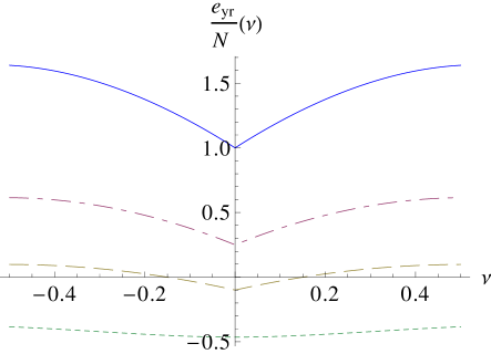
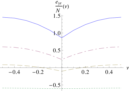
Fig. 2: Top: variational intrinsic yrast energies per particle (in units of $\hbar^{2}/2MR^{2}$) as a function of $\nu=(L-Nl)/N$ for $g=2$ (full line), $g=0.5$ (dot-dashed), $g=-0.2$ (dashed) and g=-0.8 (dotted). The cusp minimum at $\nu=0$ is typical for $g>-0.5$. Extending the plot to $\nu>0.5$ (or to $\nu<-0.5$) by using periodicity generates a cusp maximum at half-integer values of $\nu$. This results from deterioration of the adopted variational ansatz away from the integer values of the abscissa. Bottom: results obtained by numerical diagonalization, with $N=10$, $l_{b}=3$ and $m_{0}=0$, for the same quantities and for the same values of $g$ on the left hand side.

A chart of the relevant minima of the intrinsic energy functional is shown in fig. 1, and numerical results for the variational intrinsic yrast energies are displayed in fig. 2. For values of the coupling constant $g$ greater than -0.5 one gets the cusp minimum at $\nu=0$, which translates also to all integer values of $L/N$, at which the minimizer condensate $|\Psi\rangle$ has good total angular momentum $L=Nl$. For values of $g$ smaller than $-0.5$, the absolute minima at $\nu=0$ have $|c_{0}|^{2}<1$ implying that in this domain one has $|c_{\pm 1}|\neq 0$, so that the minimizer breaks the rotational symmetry. This signals a quantum phase transition at $g=-0.5$, as pointed out in ref. [7] in connection with the ground ($L=0$) state. Furthermore, as $g$ is decreased below the transition value, calculated yrast intrinsic energies become very weakly dependent on $\nu$. Consequently, the yrast line essentially reduces in this domain of values of $g$ to a rotational band with the rigid moment of inertia. Further insight into the yrast states in this phase will be drawn from results of the numerical diagonalization of the model Hamiltonian (4), to be discussed below.

4.1 Persistent currents.

It was argued by Bloch[5] that the occurrence of minima at non vanishing values of the angular momentum along the yrast line indicated meta-stability of the associated current against additional couplings allowing for exchange of angular momentum between the system and its surroundings. The above variational results show that such minima will in fact develop at integer values of $L/N$, albeit as cusp minima, whenever the coupling parameter $g$ is large enough to make the right-slope of the cusps shown in fig. 2 larger than the slope of the center of mass energy at the corresponding value of $L/N$. Having in mind the periodicity and symmetry properties of the intrinsic yrast energies, it is in fact easy to see that cusp minima will in this case appear in the yrast line itself. Quantitative predictions of the values of $g$ at which this happens for the three lowest integer values of $L/N$ are shown in fig. 3.

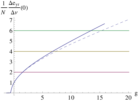
Fig. 3: The dashed curve shows the value of the slope $\frac{1}{N}\frac{\Delta e_{yr}}{\Delta\nu}$ at $\nu=0$ (in units of $\hbar^{2}/2MR^{2}$) as function of $g$, and the horizontal lines show the values of the slope of the center of mass energy per particle for $L/N=1,2$ and $3$. In view of the periodicity and symmetry properties of the intrinsic energies, the intercepts indicate the values of $g$ above which cusp minima develop at these values of $L/N$, indicating meta-stability of the currents in the sense proposed by Bloch[5]. The full line curve shows the corresponding results obtained by diagonalizing the Hamiltonian (4) for $N=40$, $l=0$ and $l_{b}=2$ (5 single-particle states). The variational slopes have been obtained numerically using an increment $\Delta\nu=1/40$ to conform to the discreteness in the diagonalization calculation.

It is worth noting explicitly that the meta-stability criterion, based on the persistence of local yrast minima in the present model, actually refers to what may be called ‘one-dimensional meta-stability’, as it depends in an essential way on the assumption that the transverse degrees of freedom in the quasi-one-dimensional system are effectively frozen. However, a simple qualitative observation which can be made concerning the $L$-values at which instabilities appear to become an experimentally limiting factor for the observation of persistent currents[2, 3] is that they occur where the de Broglie wavelength is no longer much larger than the transverse scale of the employed toroidal trap, which would allow for the participation of additional degrees of freedom in the dynamics of angular momentum transfer. Also, in these experiments, the values of the coupling constant $g$ can be estimated to be of the order of thousands, indicating persistence of ‘one-dimensional meta-stability’ for values of $L$ up to about two orders of magnitude above the largest reported observed value. A realistic appraisal of the decay of the macroscopically quantized angular momentum of the persistent currents is therefore beyond the bearings of the present model.

5 Characterization of the yrast line II - numerical diagonalization.

For not too large a number of particles the stationary states of the Hamiltonian (4) can be obtained by direct numerical diagonalization in a truncated base of many-body state vectors. Taking advantage of the fact that the total angular momentum is a constant of motion, one may consider for each value of $L$ the truncated base formed by the set of $N$-body state vectors

$${\prod_{m}}^{\prime}\frac{1}{\sqrt{m!}}(b_{m}^{\dagger})^{n_{m}}|0\rangle$$ (12)

with $l-l_{b}\leq m\leq l+l_{b}$, $\sum_{m}n_{m}=N$ and $\sum_{m}mn_{m}=L$. The value of $l$ plays here the same role as in eq. (8), i.e. shifting the central value of the selected band of $2l_{b}+1$ single particle angular momentum functions in order to optimize the base for the relevant value of $L$, taking into account the periodicity and symmetry properties of the intrinsic spectrum. The $n_{m}$ are occupation numbers for the single particle states $m$. We report on calculations involving values of $N$ from 10 to 40, and bases involving from 5 $(l_{b}=2)$ to 11 $(l_{b}=5)$ single-particle states. Due to the periodicity of the (non-trivial) intrinsic spectrum, we set $l=0$ without loss of generality. It is worth noting that, for a given number of particles $N$, the truncation involved in the adoption of a given set of single particle states leads to many-body subspaces with good $L$ having different dimensionalities, implying a small residual $L$ dependence of the truncation effects on the many-body eigenfunctions and energy eigenvalues. The latter are in any case variational upper bounds to the ‘true’ eigenvalues for each value of $L$.

The value of the effective two-body interaction strength parameter $\Lambda$ is always taken, in the numerical diagonalizations, to be related to the strength parameter $g$ used in connection with the variational treatment as

$$\Lambda=\frac{\hbar^{2}}{2MR^{2}}\frac{g}{N-1}$$ (13)

with the understanding that different particle numbers $N$ are dealt with by adjusting $\Lambda$ so as to keep the value of $g$ constant, as this will tend to preserve the ‘ground state phase diagram’ of the system as $N$ is varied. This is indeed an exact feature of the variational approach, but holds only approximately when one carries out many-body diagonalizations, as shown explicitly in fig. 4, which compares the variational energy per particle for the $L=0$ ground state evaluated variationally for some sample values of $g$ and the corresponding $N$-dependent energies per particle obtained by diagonalization in many-body bases built on a set of single-particle orbitals with $l=0$ and $l_{b}=2$.

Fig. 4: Variational $L=0$ ground state energies per particle for $g=-1.0,\;-0.2,\;1.0$ and $5.0$ (dashed lines, from the bottom up) and the corresponding $L=0$ ground state energies per particle obtained by numerical diagonalization for a range of values of $N$ using the prescription (13). The many-body bases are constructed from a set of single particle orbitals with $l=0$ and $l_{b}=2$ (see (12)).

Intrinsic yrast energies obtained in this way are shown in fig. 2 together with the corresponding variational results, showing the very good overall agreement of the two evaluations, even though the diagonalization is performed for a small system ($N=10$). It should be kept in mind that, in view of the truncation of the base the reported yrast energy results actually provide upper bounds for the ‘actual’ yrast energies; and that, for results obtained using many-body bases constructed from a fixed set of single-particle orbitals, truncation effects are apt to increase as one moves away from the cusp at $\nu=0$. In particular, residual $L-$dependence of the intrinsic yrast energies $e_{\rm yr}$ in the deformed domain $g<-0.5$ is reduced as $l_{b}$ (i.e., the number of single-particle orbitals involved in the construction of the many-body base vectors) is increased.

The predicted values of $g$ at which the cusps generate yrast minima indicating the onset of meta-stable currents at integer values of $L/N$ can be read from the values of $de_{\rm yr}(0)/d\nu$ shown as the full line curve of fig. 3. Comparison with the values obtained from the variational dashed curve reveal that the truncated diagonalization results in deeper cusp minima, leading to smaller critical values of $g$ notably for $L/N\geq 2.$

6 Probing correlated states.

The availability of correlated many-body yrast state vectors obtained from many-body diagonalizations allows for further probing of the variational transition at $g=-0.5$. As found also in the variational calculation, numerical diagonalizations in this domain reveal a regime in which the intrinsic yrast energies become essentially independent of $\nu=L/N-l$, the yrast line approaching a rotational band whose moment of inertia is essentially the rigid moment of inertia. Note that the intrinsic energies for different values of $\nu$ correspond now to diagonalizations carried out in orthogonal many-body subspaces, dynamically decoupled by symmetry. This suggests that the quantum phase transition identified through the breaking of the rotational symmetry of the variational ground state is akin to the onset of ‘intrinsic deformations’ in nuclear and molecular spectra displaying well developed rotational bands.

Fig. 5: Angular momentum transfer matrix elements between yrast states with successive angular momentum values as a function of the coupling strength $g$ for $N=14$. The different curves correspond to different values of $L$. The value of the matrix elements for non interacting particles $(g=0)$ comes from bosonic enhancement factors and are respectively 14, 26, 36, 44, 50 54 and 56 for $L=$ 0 to 6. The onset of the deformed phase for $g<-0.5$ is accompanied by a large enhancement of these matrix elements.

As one way of scrutinizing this interpretation, one may take advantage of the good angular momentum eigenstates resulting from the numerical diagonalization procedure in order to detect collective behavior in appropriate transition matrix elements[10]. A simple and effective choice in this connection is to evaluate matrix elements between successive yrast states of the angular momentum transfer operator

$$T_{1}\equiv\sum_{m=l-l_{b}}^{l+l_{b}-1}\left(b^{\dagger}_{m+1}b_{m}+b_{m}^{\dagger}b_{m+1}\right).$$

Matrix elements of this operator between yrast states for a range of values of the coupling strength parameter $g$ are shown in Fig. 5 for states with particle number $N=14$. A strong enhancement above the values involving just bosonic factors (which alone determine the matrix elements at $g=0$) sets in sharply in the deformed domain $g<-0.5$. For $g>0$, on the other hand, the free particle values are quenched by the correlations induced by the effective two-body interaction. To the extent that operators involving $T_{1}$ are involved in the loss of angular momentum trough external couplings, this provides an indication that this type of loss is hindered by the correlations induced by repulsive two-body interactions.

As a second approach, one may use the numerical correlated eigenstates to evaluate appropriate correlation functions. We focus in particular on the correlation functions

$$\frac{\langle\Psi_{E_{L}}|\psi^{\dagger}(\varphi)\psi^{\dagger}(\varphi^{\prime})\psi(\varphi^{\prime})\psi(\varphi)|\Psi_{E_{L}}\rangle}{{\rm Tr}\langle\Psi_{E_{L}}|\psi^{\dagger}\psi^{\dagger}\psi\psi|\Psi_{E_{L}}\rangle}\equiv\rho^{(2)}_{E_{L}}(\varphi-\varphi^{\prime})$$ (14)

where the states $|\Psi_{E_{L}}\rangle$ are yrast states. Results for this function are shown in fig. 6 for $g=1.$ and for $g=-1.$ While in the first case there is a clear dependence on the value of the angular momentum (together with some tendency to anti-correlation, as signaled by the relatively shallow minima at $\varphi-\varphi^{\prime}=0$), in the attractive case the correlation function is essentially independent on the value of the angular momentum, being strongly peaked at $\varphi-\varphi^{\prime}=0$ and dropping to very small values at $\varphi-\varphi^{\prime}=\pm\pi$ consistently with the correlation expected as a result of the attractive character of the effective interaction.

Fig. 6: Dashed curves: Nearly isotropic two-body correlation functions at $g=1$ for the yrast states with $L=0$ to $5$ (lowest to upper curve at $\varphi-\varphi^{\prime}=0$), using many-body states obtained from a diagonalization of the Hamiltonian (4) with $N=10$, $l=0$, $l_{b}=4$ (see (12)). Full curves: Same as the dashed curves but at $g=-1.$ Note in this case the strong anisotropy and the weaker angular momentum dependence of the correlation functions.

Fig. 7: Logarithm (for clarity in the display of smaller values) of the mean single particle occupation numbers $\langle n\rangle_{m}$, for a system with $N=10$ treated in the many-body base constructed from single-particle orbitals with $l=0$ and $l_{b}=5$ (see (12)), plotted against the single particle angular momentum $m$. The plot on top has been calculated with a repulsive effective interaction $g=2.0$ and displays results for the $L=0$ (filled circles, full line) and $L=5$ ($L/N=0.5$, crosses, short-dashed line). The open circles connected by a long-dashed line are those corresponding to $L/N=0.5$ displaced by $-0.5$ along the $m$ axis. The bottom graph shows the corresponding plots for an attractive effective interaction with $g=-2.0$. Unlike in the case of the repulsive interaction, here the points obtained for $L/N=0.5$, after translation by $-0.5$ along the $m$ axis, essentially fall on the same curve as the $L=0$ occupations.

The stiffness of the two-body correlation function with respect to changes of angular momentum in the ‘deformed’ phase in fact leaves an imprint also in the one-body reduced density matrix

$$\langle\Psi_{E_{L}}|b^{\dagger}_{m^{\prime}}b_{m}|\Psi_{E_{L}}\rangle=\rho^{(1)}_{E_{L}mm^{\prime}}=\langle n\rangle_{m}\;\delta_{mm^{\prime}}$$

whose eigenvalues, written as $\langle n\rangle_{m}$, are the mean occupation numbers of the single particle orbitals $\phi_{m}(\varphi)$. As illustrated in fig. 7, in the deformed regime the eigenvalues of the one body density for yrast states with different angular momenta fall essentially on a single distribution curve, after being translated by the fractional value of $L/N$. This is at variance with what one finds in the non-deformed regime, where a considerable fraction of the particle number $N$ is carried by the $m=0$ orbital consistently with the relatively small anisotropy of the two-body correlation function in this case.

6.1 Yrast many-body correlations.

Finally, one may consider the full ‘intrinsic wave functions’ $\chi_{N,L}(\varphi_{1},\dots,\varphi_{N})$ defined by Bloch by factoring out from the yrast wave functions $\Psi_{N,L}$ ‘center of mass factors’ for the given number of particles $N$ and for each value of $L$, i. e.

$$\Psi_{N,L}(\varphi_{1},\dots,\varphi_{N})=e^{i\frac{L}{N}\sum_{j=1}^{N}\varphi_{j}}\chi_{N,L}(\varphi_{1},\dots,\varphi_{N})$$

These intrinsic wave functions depend only on coordinate differences $\varphi_{j}-\varphi_{k}$ and are therefore rotationally invariant. They satisfy the ‘twisted’ boundary conditions

$$\chi_{N,L}(\varphi_{1},\dots,\varphi_{j}+2\pi,\dots,\varphi_{N})=e^{-2\pi i\frac{L}{N}}\chi_{N,L}(\varphi_{1},\dots,\varphi_{j},\dots,\varphi_{N}).$$

Since they are rotationally invariant, the intrinsic wave functions are eigenfunctions of the total angular momentum with eigenvalue zero, so that they are also eigenfunctions of $H$ with eigenvalue $e_{\rm int}^{(L)}$.

In order to access the intrinsic wave functions for each of the values of the total angular momentum $L$ within the second-quantization framework adopted here we first consider the description of the system in a frame of reference which rotates with angular velocity $\Omega$ about the axis of the toroidal configuration space. The corresponding Hamiltonian $H_{\Omega}$ is related to $H$, as written in eq. (1), by making the replacement $l_{z}^{2}\rightarrow(l_{z}-MR\Omega/\hbar)^{2}$ in the kinetic energy term. The terms involving $\Omega$ may furthermore be eliminated by means the gauge transformation of the field operators $\psi(\varphi)\equiv e^{i\frac{MR^{2}\Omega}{\hbar}\varphi}\psi^{\prime}(\varphi)$, which leads to the simpler form of $H_{\Omega}$ involving the ‘twisted’ field operators $\psi^{\prime}(\varphi)$

$$H_{\Omega}=\frac{\hbar^{2}}{2MR^{2}}\int_{0}^{2\pi}d\varphi\psi^{\prime\,\dagger}(\varphi)l_{z}^{2}\psi^{\prime}(\varphi)++\frac{1}{2}\frac{U_{c}}{RS}\int_{0}^{2\pi}\psi^{\prime\,\dagger}(\varphi)\psi^{\prime\,\dagger}(\varphi)\psi^{\prime}(\varphi)\psi^{\prime}(\varphi)d\varphi.$$

Consider next the representation of this Hamiltonian in the orthonormal twisted single-particle base with vectors

$$\phi_{m}^{\Omega}(\varphi)=\frac{1}{\sqrt{2\pi}}e^{i\left(m-\frac{MR^{2}\Omega}{\hbar}\right)\varphi}\;,\hskip 14.22636pt\frac{1}{2\pi}\int_{0}^{2\pi}d\varphi\;\phi_{m^{\prime}}^{\Omega\,*}(\varphi)\phi_{m}^{\Omega}(\varphi)=\delta_{mm^{\prime}}$$ (15)

by expanding the field operators as

$$\psi^{\prime}(\varphi)=\sum_{m}\phi_{m}^{\Omega}(\varphi)\beta^{\Omega}_{m}.$$ (16)

The resulting expression for the second quantized Hamiltonian in the rotating frame is therefore

$$H_{\Omega} = \frac{\hbar^{2}}{2MR^{2}}\sum_{m}\left(m-\frac{MR^{2}\Omega}{\hbar}\right)\beta^{\Omega\,\dagger}_{m}\beta^{\Omega}_{m}+$$

$$\hskip 56.9055pt+\frac{\Lambda}{2}\sum_{m_{i}}\beta^{\Omega\,\dagger}_{m_{1}}\beta^{\Omega\,\dagger}_{m_{2}}\beta^{\Omega}_{m_{3}}\beta^{\Omega}_{m_{4}}\delta_{m_{1}+m_{2},m_{3}+m_{4}}.$$

Particle number and the total angular momentum remain constants of motion.

When considering states with with $N$ particles and total angular momentum $L$, the choice $\Omega\rightarrow\Omega_{NL}\equiv\hbar L/(NMR^{2})$ reduces the gauge term to just $L/N$. With this choice, in the $N$, $L$ sector of the Fock space the Hamiltonian $H_{\Omega}$ reduces to to the form $(\ref{Hbase})$ with the $b$-operators replaced by twisted $\beta$-operators, and with the subtraction of the center of mass energy $\hbar^{2}L^{2}/(2NMR^{2})$. Thus, except for the trivial subtraction of a multiple of the unit matrix related to the center of mass energy, it is represented in the basis of twisted many-body state vectors vectors (cf. eq. (12))

$$\prod_{m}\frac{1}{\sqrt{m}}(\beta_{m}^{N,L\;\dagger})^{n_{m}}|0\rangle,\hskip 14.22636pt\sum_{m}n_{m}=N,\;\,\sum_{m}mn_{m}=L$$

by the same numerical matrix obtained in connection with the Hamiltonian (4) using the many-body states (12).

This identifies the numerical ground state in the twisted $N$, $L$ sector as the yrast ‘intrinsic state’ for the selected values of $N$ and $L$. The ‘intrinsic states’ are therefore just of the form (7), with the same coefficients $C^{(j)}_{\{n_{m}\}_{N,L}}$, but with the $N$-body base vectors expressed in terms of the ‘twisted’ bosonic operators $\beta^{\Omega_{NL}}_{m}$, $\beta^{\Omega_{NL}\,\dagger}_{m}$, i.e.

$$|\Psi^{\rm int}_{e^{(L)}_{\rm int}}\rangle=\sum_{\{n_{m}\}_{N,L}}C^{(0)}_{\{n_{m}\}_{N,L}}\prod_{m}\frac{1}{\sqrt{n_{m}!}}\left(\beta^{\Omega_{NL}\,\dagger}_{m}\right)^{n_{m}}|0\rangle.$$

The fact that they correspond to rotationally invariant amplitudes in configuration space is borne out by the fact that $\sum_{m}n_{m}(m-L/N)=0$. It should be stressed that intrinsic states corresponding to different values of the total angular momentum $L$ will not be orthogonal, since they are eigenvectors of differently twisted Hamiltonians.

Fig. 8: Top: Eigenvalues $\lambda_{n}$ of the overlap matrix of many-body intrinsic states for $N=14$, $L=-7$ to $6$ as functions of the coupling strength $g$. The values plotted are normalized by the trace ($\sum\lambda_{n}=14$) of the overlap matrix. Bottom: Squared amplitudes along intrinsic states with different $L$-values of the eigenvector associated with the largest eigenvalue of the overlap matrix as functions of $g$. The numerical many-body eigenstates used to generate the overlap matrix were evaluated using the full many-body base constructed in terms of five single-particle orbitals with $l=0$ and $l_{b}=2$ (see (12)).

These rotationally invariant intrinsic yrast states can be used, in particular, to provide for indications concerning the nature of the quantum phase transition at $g\simeq-0,5$. The simplest information which may be derived from these non-orthogonal states is the content and hierarchy of the domain of the many-body phase space spanned by them. For the purpose of obtaining it we take the set of yrast intrinsic states associated with one period, i. e. $-\frac{1}{2}\leq\frac{L}{N}<\frac{1}{2}$, and evaluate their overlap matrix

$$\Omega^{(N)}_{L,L^{\prime}}=\langle\Psi^{\rm int}_{e^{(L)}_{\rm int}}|\Psi^{\rm int}_{e^{(L^{\prime})}_{\rm int}}\rangle.$$ (17)

This is done using the commutators

$$\left[\beta^{N,L}_{m},\beta^{N,L^{\prime}\;\dagger}_{m^{\prime}}\right]=\left(\phi^{N,L^{\prime}}_{m^{\prime}}|\phi^{N,L}_{m}\right)\equiv\int_{0}^{2\pi}d\varphi\phi^{N,L^{\prime}\,*}_{m^{\prime}}(\varphi)\phi^{N,L}_{m}(\varphi)$$

which involve the unitary transformation between different twisted single particle bases, these being defined in eq. (15). Diagonalizing the overlap matrix, i.e.

$$\sum_{L^{\prime}}\Omega^{(N)}_{LL^{\prime}}f^{(n)}_{L^{\prime}}=\lambda_{n}f^{(n)}_{L},\hskip 14.22636pt{\rm with}\hskip 14.22636pt\sum_{L}f^{(n)*}_{L}f^{(n^{\prime})}_{L}=\delta_{nn^{\prime}}$$

so that

$$\Omega^{(N)}_{LL^{\prime}}=\sum_{n}\lambda_{n}f^{(n)}_{L}f^{(n)*}_{L^{\prime}},$$

we see that the eigenvectors $f^{(n)}$ identify ‘principal directions’ in the many-body phase space, as their components $f^{(n)}_{L}$ represent amplitudes of each principal direction on the different intrinsic states. The associated eigenvalues $\lambda_{n}$, on the other hand, specify weights identifying the participation of each one of the principal directions in the set of intrinsic states.

The effect of the onset of deformation on the set of intrinsic states is borne out in terms of these ingredients in Fig. 8. The upper part of this figure shows a plot of the relative weight of the largest eigenvalue $\lambda_{0}$ of the overlap matrix as function of the coupling constant $g$, while the lowest part plots squared components $|f^{(0)}_{L}|^{2}$ of the eigenvector associated to the largest eigenvalue along the intrinsic states. A clear transition is seen to occur in the spectrum of the overlap matrix when the value of the coupling constant is reduced in the vicinity of $g=-0.5$. In the domain with stronger attractive coupling a single state acquires dominance over the content of the intrinsic subspace, as revealed by the fact that the corresponding eigenvalue exhausts an important fraction of the trace. This indicates that the yrast states in the ‘deformed phase’, at $g<-0.5$, are at least strongly dominated by a single, common many-body correlation function. A change of regime is also noted in the $L$-composition of the dominant eigenvector, which becomes uniformly flat in the ‘deformed’ region, as shown also in Fig. 8. This indicates that the dominant, common intrinsic state is a nearly uniform superposition of the intrinsic states for the various $L$-values present in the intrinsic yrast period.

The features shown in Fig. 8 for $N=14$ particles are found also for smaller values on $N$, albeit with a strengthening of the single state dominance. This may be attributed at least in part to limitations imposed by the truncation of the twisted bases on the numerical evaluation of the many-body intrinsic overlaps. Indeed the truncation is apt to fail to saturate the unitarity relations assumed in the evaluation of the overlaps. Because of this, the calculated value of the dominant eigenvalue should be considered as a lower bound.

7 Concluding remarks.

We have examined a particular realization of the one-dimensional model system considered long ago by F. Bloch[5]. It involves ingredients drawn from current experimental and theoretical research involving trapped, dilute atomic gases. In particular, the usual effective contact two-body interaction based on the atom-atom scattering length and its quasi one-dimensional reduction involving the trap geometry have been explicitly used. The main focus is the quantum dynamics of finite many-body systems, in which invariance under rotations and global gauge transformations play a fundamental role in establishing relevant dynamic cleavages between subspaces of the many-body phase space with different values of total angular momentum and particle number. In this context, the phenomena of persistent, meta-stable currents and of ‘deformations’, as revealed by collective rotational features, appear as emergent properties developing across the cleavages imposed by symmetry through the onset of appropriate correlation properties. A natural domain hosting such emergence is the set of yrast states, the lowest energy states for each value of the total angular momentum.

The properties of the yrast states resulting from a variational mean-field approach allowing for the control of the mean total angular momentum, which amounts to a restricted mean field approximation, have been confronted to correlated many-body stationary states resulting from a many-body diagonalization in truncated Fock subspaces with good particle number and angular momentum.

The effects of a sufficiently strong repulsive two-body effective interactions appear in both cases as essential for the generation of the yrast energy minima which can be associated with meta-stability of persistent currents[5, 11]. The relevant minima appear as yrast cusps at values of the total angular momentum which are integer multiples of the particle number. Threshold two-body interaction values for the occurrence of actual minima at a given integer value of the total angular momentum per particle become rather insensitive to particle number $N$ when scaled by $1/N$, as this maintains the balance of the kinetic and interaction effects in the effective Hamiltonian.

In the case of attractive two-body effective interactions, and within the variational restricted mean-field approach, the ‘quantum phase transition’ pointed out in ref. [7] manifests itself, as usual, in terms of a self-consistence related breaking of the rotational symmetry of the ground state. This is moreover accompanied by the disappearance of the yrast cusps, which are replaced by analytic, locally quadratic yrast minima together with the overall flattening of the intrinsic yrast energies. This behavior of the intrinsic yrast energies is borne out also in the case of the diagonalization results. Since they rely on the use of subspaces of good particle number and angular momentum, properties related to the quantum phase transition must be sought in the correlation properties of many-body states. In fact not only the behavior of two-body correlation functions of the yrast states undergoes profound changes as one crosses the transition region, but further standard characteristics of collective ‘deformations’[10] also arise there. In fact we find both a strong ‘collective’ enhancement of transition matrix elements of a one-body angular momentum transfer operator acting between neighboring members of the yrast line and the emergence of a weighty common eigen-component in the many-body subspace generated by the intrinsic yrast states. The individual intrinsic yrast states are themselves rather uniformly represented in this common eigen-component, as can be seen in figure 8. The full ‘deformation syndrome’, present notably in the dynamics of the much more complex molecular and nuclear systems, appears thus to be deployed in the present one-dimensional model. The simplicity of the model makes the associated correlation structures more accessible to detailed scrutiny.

Acknowledgement. We acknowledge useful discussions with João C. A. Barata.

References

- [1] A. Ramanathan, K. C. Wright, S. R. Muniz, M. Zelan, W. T. Hill III, C. J. Lobb, K. Helmerson, W. D. Phillips and G. K. Campbell, Phys. Rev. Lett. 106, 130401 (2011); S. Beattle, S. Moulder, R. J. Fletcher and Z. Hadzibabic, Phys. Rev. Lett. 110, 025301 (2013); K. C. Wright, R. B. Blakestad, C. J. Lobb, W. D. Phillips and G. K. Campbell, Phys. Rev. Lett. 110, 025302 (2013).
- [2] S. Moulder, S. Beattle, R. P. Smith, N. Tammuz and Z. Hadzibabic, Phys. Rev. A86, 013629 (2012);
- [3] N. Murray, M. Krygier, M. Edwards,K. C. Wright, G. K. Campbell and C. W. Clark, Phys. Rev. A88,053615 (2013).
- [4] A. Bohr and B. Mottelson, Phys. Rev. 125, 495 (1962).
- [5] F. Bloch, Phys. Rev. A7, 2187 (1973).
- [6] F. Bloch, Phys. Rev. Lett. 17, 1241 (1968).
- [7] Rina Kanamoto, Hiroki Saito and Masahito Ueda, Phys. Rev. A67, 013608 (2003).
- [8] G. M. Kavoulakis, Phys. Rev. A67, 011601(R) (2003); Phys. Rev. A69, 023613 (2004).
- [9] Rina Kanamoto, Hiroki Saito and Masahito Ueda, Phys. Rev. A68, 043619 (2003), Rina Kanamoto, Lincoln D. Carr and Masahito Ueda, Phys. Rev. Lett. 100, 061401 (2008) and Phys. Rev A79, 063616 (2009), K. Anoshkin, Z, Wu and E. Zaremba, Phys. Rev. A88, 013609 (2012), M. Abad, A. Sartori, S. Finazzi and E. Recati, Phys. Rev. A89 053602 (2014).
- [10] A. Bohr and B. R. Mottelson, Nuclear Structure v.2. - Nuclear Deformations, W. A. Benjamin, Inc. (1975).
- [11] A. J. Leggett, Revs. Mod. Phys. 73, 307 (2001).
- [12] B. Mottelson, Phys. Rev. Lett. 83, 2695 (1999).
- [13] While this obviously the case for the standard contact effective interaction adopted in eqs. (1) and (4), it remains true under the weaker condition of rotational invariance of the two-body interaction term[5].
- [14] This particular strategy in connection with the dependences on the number of particles of the parts on the Hamiltonian can be seen as akin to the ‘Gross-Pitaevski limit’ adopted in a 3-D context by Lieb and collaborators, see E. H. Lieb, R. Seiringer, J. P. Solovej and J. Yngvason, the Mathematics of The Bose Gas and its Condensation, Birkh user 2005, section 6.1