On the Whittle Index for Restless Multi-armed Hidden Markov Bandits

Abstract

We consider a restless multi-armed bandit in which each arm can be in one of two states. When an arm is sampled, the state of the arm is not available to the sampler. Instead, a binary signal with a known randomness that depends on the state of the arm is available. No signal is available if the arm is not sampled. An arm-dependent reward is accrued from each sampling. In each time step, each arm changes state according to known transition probabilities which in turn depend on whether the arm is sampled or not sampled. Since the state of the arm is never visible and has to be inferred from the current belief and a possible binary signal, we call this the hidden Markov bandit. Our interest is in a policy to select the arm(s) in each time step that maximizes the infinite horizon discounted reward. Specifically, we seek the use of Whittle’s index in selecting the arms.

We first analyze the single-armed bandit and show that in general, it admits an approximate threshold-type optimal policy when there is a positive reward for the ‘no-sample’ action. We also identify several special cases for which the threshold policy is indeed the optimal policy. Next, we show that such a single-armed bandit also satisfies an approximate-indexability property. For the case when the single-armed bandit admits a threshold-type optimal policy, we perform the calculation of the Whittle index for each arm. Numerical examples illustrate the analytical results.

I Introduction

Restless multi-armed bandit problems are a generalization of the classical multi-armed bandit (MAB) problem. In the MAB, the sampler chooses one of $N$ arms in each time-step and receives a reward. Each arm can be in one of $M$ states and the reward is dependent on the state of the arm. The sampled arm changes state according to a known law while the other arms are frozen. In the RMAB, all the arms change their state at each time-step, i.e., the arms are restless. The law that governs the change of state could depend on whether the arm was sampled or not sampled. In this paper we introduce a class of RMAB problems where the player never gets to observe the state of the arm. The objective in both MAB and RMAB is to choose the sequence of arms to sample so as to maximize a long term reward function. We begin with two motivating examples for the models that we introduce in this paper.

I-A Motivation

Opportunistic access in time-slotted multi-channel communication systems for Gilbert-Elliot channels [1] is being extensively studied. In the typical model there are $N$ channels and each channel can be in one of two states—a good state and a bad state. Each channel independently evolves between these two states according to a two-state Markov chain. The sender can transmit on one of these $N$ channels in each time slot. If the selected channel is in the good state, then the transmission is successful, and if it is in the bad state, it is unsuccessful. The sender receives instantaneous error-free feedback about the result of the transmission in both these cases. If the sender knows the transition probabilities of the channels, then using the feedback, it can calculate a ‘belief’ for the state of each channel in a slot. This belief may be used to select the channel in each slot to optimize a suitable reward function. This system and its myriad variations have been studied as restless multi-armed bandit (RMAB) problems.

Consider a system as above except that now the probability of success in the good state and of failure in the bad state are both less than one and the sender knows these probabilities. This generalization of the Gilbert-Elliot channel means that the sender does not get perfect information about the state of the channel from the feedback. However, it can update its a posteriori belief about the state of the channel based on the feedback, and use this updated belief in the subsequent slot.

As a second motivating example, consider an advertisement (ad) placement system (APS) for a user in a web browsing session. Assume that the APS has to place one ad from $M$ candidate ads each of which has a known click-through probability and an expected reward determined from the user profile. It is conceivable that the click-through probabilities for ads in a session depend on the history of the ads shown; users often react differently depending upon the frequency with which an ad is shown. Some users may, due to annoyance, respond negatively to repeated display of an ad, which has the effect of lowering the click-through probability if they were shown this ad in the past. Others may convert disinterest to curiosity if an ad is repeated thereby increasing the click-through probability. Yet other users may be more random or oblivious to what has been shown, and may behave independently of the history.

The effect of recommendation history on a user’s interest can be modeled as follows. A state is associated with each ad and the state changes at the end of each session (the state intuitively signifies the interest level of the user in the ad). The transition probabilities for this change of state depend on whether the ad is shown or not shown to the user in the session. Assume that the state change behavior is independent of the past and of the state change of the other ads. Each state is associated with a value of click-through probability and expected revenue. The state transition and the click-through probabilities determine the ‘type’ or profile of the user. In each session the APS only observes a ‘signal’ or outcome (click or no-click) for the ad that it displayed and no signal for those that are not displayed. The action and the outcome is used to update its belief about the current state of the user for each ad. The objective of the APS would be to choose the ad in each session that optimizes a long term objective. Clearly, this is also a RMAB with the added generalization that the transition probabilities for the arms depend on the action in that stage.

In this paper we analyze this generalization of the restless multi-armed bandit—the states are never explicitly observed and the transition probabilities depend in general on the action chosen. To the best of our knowledge, such systems have not been considered in the literature.

I-B Literature Overview

Restless multi-armed bandits (RMAB) are a special class of partially observed Markov decisions processes (POMDPs) and are in general PSPACE-hard [2], but many special cases have been studied. An important recent application of RMABs is in dynamic spectrum access systems, e.g., [3, 4, 5, 6]. A common channel shared by many heterogeneous users, each of whom see the channel as an independent Gilbert-Elliott channel is considered in [3] where an index-based policy to maximize the discounted infinite-horizon throughput minus the transmission costs is derived. In [4], the occupancy of channels by primary users is modeled as a two-state Markov chain. The secondary users (SUs) sense the channel using error-prone spectrum sensors before transmitting. Again, an index policy to maximize the infinite-horizon discounted throughput is derived. In [5], the objective is similar to that of [3] and it is shown that a Whittle’s index based policy is optimal. In [6] multiple service classes are considered and the objective is to maximize a utility function based on the queue occupancies. Conditions for a myopic policy, based on instantaneous reward, to be optimal are derived. Myopic policies are also the subject of interest in several other recent works, including [7, 8, 9]. Utility functions are used in [10] that considers a system similar to that of [5]. Opportunistic spectrum access as POMDPs are also studied in [11, 12, 13].

In much of the restless multi-armed bandit literature, including the references in the preceding, the solution method is to seek an ‘index-based’ policy where the state of each arm is mapped to an index and at each step the arms with the highest index values are played. Whittle’s index, first proposed in [14], is based on a Lagrangian relaxation and decomposition and is a popular one; see e.g., [15, 16, 5, 17, 18, 19]. An alternative indexing scheme is based on partial and generalized conservation laws [20] and on marginal productivity [4]; in this paper, we will concentrate on the Whittle index. The first step in determining if an index-based policy can be used is to prove indexability. Whittle indexability is shown by analyzing the one armed bandit as a POMDP, the analyses of which borrows significantly from early work on POMDPs that model machine repair problems like in [21, 22, 23]. These are described next.

In [21], a machine is modeled as a two-state Markov chain with three actions and it is shown that the optimal policy is of the threshold type with three thresholds. In [23], a similar model is considered and the formulas for the optimal costs and the policy are obtained. This and some additional models are considered in [22] and, once again, several structural results are obtained. Also see [24] for more such models.

The key features in the single-arm problems considered in the preceding are as follows. One or more of the actions provides the sampler with exact information about the state of the Markov chain. Furthermore, the transition probability of the state of the arms does not depend on the action. These are also the features of each of the arms of the RMAB models discussed earlier. In this paper we consider a model that drops both these restrictions. Since the state is never observed but only estimated from the signals when the arm is sampled, our model can be called a ‘hidden Markov restless multi-armed bandit.’ A rested hidden Markov bandit has been studied in [25], where the state of an arm does not change if it is not sampled. The (arguably simpler) information structure in a hidden rested bandit admits an analytical solution via Gittins indices.

A further simplification that is often made in showing indexability is to assume, without a formal proof, the existence of a threshold-type optimal policy for the single-arm case, i.e., it is optimal to play the arm if the state is higher than the threshold and optimal to not play if the state is below the threshold as in, e.g., [3]. Under this simplification, in many cases, the state of the arm can be mapped to an index without actually calculating the threshold. In Section V we describe a method to do this.

I-C Summary of the Contributions

We now summarize the key contributions of this paper. We consider restless multi-armed bandits in which the transition probabilities of the arms depends on whether the arm is played or not played. Although the applications for this model appear to be many, to the best of our knowledge, this is not a well-studied problem. In addition, the states of the arms are never observed and only a belief about the state of the arm can be computed using prior belief and the conditional probabilities of the observation from a play of the arm. Once again, we believe such a system has not been studied. The preceding features make the system hard to analyze using well known techniques. Hence we develop the notion of an approximately threshold type optimal policy and prove that in general the single armed bandit that we consider admits such an optimal policy. For some special cases of the system parameters we also show that the single armed bandit in fact admits a threshold-type optimal policy. We then define approximate-indexability and show that the arms defined by our model also satisfy this property. This justifies the use of Whittle’s index based policy for the restless multi-armed hidden Markov bandits. For the case when a threshold type policy is indeed the optimal policy, we outline the procedure to compute the Whittle’s index. Numerical examples illustrate the theory.

The model details are described in the next section.

II Model Description and Preliminaries

We consider the following restless, multi-armed bandit problem with $N$ arms. Time is slotted and indexed by $t.$ Each arm has two states, $0$ and $1.$ Let $X_{n}(t)\in\{0,1\}$ be the state of arm $n$ at the beginning of time $t.$ Let $A_{n}(t)\in\{0,1\}$ denote the action in slot $t$ for arm $n,$ i.e.,

$$A_{n}(t)=\begin{cases}1&\mbox{Arm $n$ is sampled in slot $t,$}\\ 0&\mbox{Arm $n$ is not sampled in slot $t.$}\end{cases}$$

We will assume that $\sum_{n=1}^{N}A_{n}(t)=1$ for all $t,$ exactly one arm is sampled in each slot. Arm $n$ changes state at the end of each slot according to transition probabilities that depend on $A_{n}(t).$ Define the following transition probabilities.

$$\mathsf{Pr}\left(X_{n}(t+1)=0|X_{n}(t)=0,A_{n}(t)=0\right) = \lambda_{n,0},$$

$$\mathsf{Pr}\left(X_{n}(t+1)=0|X_{n}(t)=1,A_{n}(t)=0\right) = \lambda_{n,1},$$

$$\mathsf{Pr}\left(X_{n}(t+1)=0|X_{n}(t)=0,A_{n}(t)=1\right) = \mu_{n,0},$$

$$\mathsf{Pr}\left(X_{n}(t+1)=0|X_{n}(t)=1,A_{n}(t)=1\right) = \mu_{n,1}.$$

In slot $t,$ if arm $n$ is in state $i$ and it is sampled, then a binary signal $Z_{n}(t)$ is observed and a reward $R_{n,i}(t,1)$ is accrued. If the arm is not sampled, then a reward $R_{n,i}(t,0)$ is accrued and no signal is observed. Let

$$\mathsf{Pr}\left(Z_{n}(t)=1\ |\ X_{n}(t)=i,A_{n}(t)=1\right)=\rho_{n,i}$$

and denote

$$R_{n,i}(t,1)=\eta_{n,i}\hskip 14.45377ptR_{n,i}(t,0)=\eta_{n,2}.$$

Fig. 1 illustrates the model and the parameters.

Arm $n$ is not sampled ($A_{n}(t)=0$)

Arm $n$ is sampled ($A_{n}(t)=1$)

Figure 1: Top: State transition probabilities, the expected reward, and the probability of binary signal 1 being observed when the arm is not sampled. Bottom: The corresponding quantities when the arm is sampled

In most applications, $Z_{n}(t)=1$ would correspond to a ‘good’ or favorable output e.g., a successful transmission or click-through in the motivating examples. Hence, we will make the reasonable assumption that $\rho_{n,0}<\rho_{n,1}$ and $\eta_{n,0}<\eta_{n,1}$ for all $n.$

Remark 1

• In the communication system example that maximizes throughput, no reward is accrued if there is no transmission. Also, in the APS example, no revenue is accrued if there is no ad displayed. Thus in both these cases, $\eta_{n,2}=0$ is reasonable.

• Further, for communication over Gilbert-Elliot channels, $\lambda_{n,i}=\mu_{n,i}$ for $i=0,1.$

We assume that $\lambda_{n,i},$ $\mu_{n,i},$ and $\rho_{n,i}$ are known. The sampler cannot directly observe the state of the arm, and hence does not know the state of the arms at the beginning of each time slot. Instead, it can maintain the posterior or belief distribution $\pi_{n}(t)$ that arm $n$ is in state $0$ given all past actions and observations, i.e., $\pi_{n}(t)=\mathsf{Pr}\left(X_{n}(t)=0\;|\;(A_{n}(s),Z_{n}(s))_{s=1}^{t-1}\right)$, and is assumed known at the beginning of slot $t.$ Thus the expected reward from sampling arm $n$ is

$$\pi_{n}(t)\eta_{n,0}+(1-\pi_{n}(t))\eta_{n,1}$$

and that from not sampling the arm is $\eta_{n,2}.$

Define the vector $\pi(t)=[\pi_{1},\ldots,\pi_{N}]\in[0,1]^{N}.$ Let $H_{t}$ denote the history of actions and observed signals up to the beginning of time slot $t$, i.e., $H_{t}\equiv(A_{n}(s),Z_{n}(s))_{1\leq n\leq N,1\leq s<t}$. In each slot, exactly one arm is to be sampled and let $\phi=\{\phi(t)\}_{t>0}$ be the sampling strategy with $\phi(t)$ defined as follows. $\phi(t):H_{t}\to\{1,\ldots,N\}$ maps the history up to time slot $t$ to the action of sampling one of the $N$ arms at time slot $t.$ Let

$$A^{\phi}_{n}(t)=\begin{cases}1&\mbox{if $\phi(t)=n,$}\\ 0&\mbox{if $\phi(t)\neq n.$}\end{cases}$$

The infinite horizon expected discounted reward under sampling policy $\phi$ is given by

$$V_{\phi}(\pi):=E\left\{\sum_{t=1}^{\infty}\beta^{t-1}\left(\sum_{n=1}^{N}A^{\phi}_{n}(t)\ (\pi_{n}(t)\ \eta_{n,0}\right.\right.$$ (1)

$$\left.+(1-\pi_{n}(t))\ \eta_{n,1}\right)+\left(1-A^{\phi}_{n}(t)\right)\ \eta_{n,2}\bigg{)}\bigg{\}}.$$

Here $\beta,$ $0<\beta<1,$ is the discount factor and the initial belief is $\pi,$ i.e.,$\mathsf{Pr}\left(X_{n}(1)=0\right)=\pi_{n}.$ Our interest is in a strategy that maximizes $V_{\phi}(\pi)$ for all $\pi\in[0,1]^{N}$

We begin by analyzing the single arm bandit in the next section. Before proceeding we state the following background lemma derived from [26] that will be useful. The proof is given in the Appendix for the sake of completeness.

Lemma 1 ([26])

If $f:\Re_{+}^{n}\to\Re_{+}$ is a convex function then for $x\in\Re_{+}^{n},$ $g(x):=||x||_{1}f\left(\frac{x}{||x||_{1}}\right)$ is also a convex function.

Notation. For sets $A$ and $B$, $A\setminus B$ is used to denote all the elements in $A$ which are not in $B$.

III Approximate Threshold Policy for the Restless Single Armed Bandit with Hidden States

For notational convenience we will drop the subscript $n$ in the notation of the previous section. Further, we will assume that $\eta_{0}=\rho_{0}$ and $\eta_{1}=\rho_{1}.$ Thus $\eta_{0}$ and $\eta_{1}$ will be in $(0,1)$ while there will be no restrictions on the range of $\eta_{2}.$ Extending the results to the case of arbitrary $\eta_{0},$ and $\eta_{1}$ is straightforward.

Recall that $\pi(t)=\mathsf{Pr}\left(X(t)=0\;|\;H_{t}\right)$ and we can use Bayes’ theorem to obtain $\pi(t+1)$ from $\pi(t),$ $A(t)$ and $Z(t)$ as follows.

1. If $A(t)=1,$ i.e., the arm is sampled, and $Z(t)=0$ then

   $$\pi(t+1)\ =\ \gamma_{0}(\pi(t))$$

   $$\hskip 10.0pt:=\ \frac{\pi(t)(1-\rho_{0})\mu_{0}+(1-\pi(t))(1-\rho_{1})\mu_{1}}{\pi(t)(1-\rho_{0})+(1-\pi(t))(1-\rho_{1})}.$$

2. If $A(t)=1$ and $Z(t)=1$ then

   $$\pi(t+1)=\gamma_{1}(\pi(t)):=\frac{\pi(t)\rho_{0}\mu_{0}+(1-\pi(t))\rho_{1}\mu_{1}}{\pi(t)\rho_{0}+(1-\pi(t))\rho_{1}}.$$

3. Finally, if $A(t)=0,$ i.e., the arm is not sampled at $t,$ then

   $$\pi(t+1)=\gamma_{2}(\pi(t)):=\pi(t)\lambda_{0}+(1-\pi(t))\lambda_{1}.$$

Recall that the policy is denoted by $\phi(t):H_{t}\rightarrow\{0,1\}$ and it maps the history up to time $t$ to one of two actions with $1$ indicating sampling the arm and $0$ indicating not sampling the arm. The following is well known [21, 27, 28]: (1) $\pi(t)$ captures the information in $H_{t},$ in the sense that it is a sufficient statistic for constructing policies depending on the history, (2) Optimal strategies can be restricted to stationary Markov policies, and (3) The optimum objective or value function, $V(\pi),$ is determined by solving the following dynamic program

$$V(\pi) = \max\left\{\rho(\pi)+\beta\left(\rho(\pi)V(\gamma_{1}(\pi))+(1-\rho(\pi))\times\right.\right.$$ (2)

$$\hskip 36.135pt\left.\left.V(\gamma_{0}(\pi))\right),\ \ \eta_{2}+\beta V(\gamma_{2}(\pi))\right\},$$

where $\rho(\pi)=\pi\rho_{0}+(1-\pi)\rho_{1}.$

Let $\pi$ be the belief at the beginning of time slot $t=1.$ Let $V_{S}(\pi)$ be the optimal value of the objective function if $A(1)=1,$ i.e., if the arm is sampled, and $V_{NS}(\pi)$ be the optimal value if $A(1)=0,$ i.e., if the arm is not sampled. We can now write the following.

$$V_{S}(\pi) = \rho(\pi)+\beta\left(\rho(\pi)V(\gamma_{1}(\pi))\right.$$ (3)

$$\hskip 20.0pt\left.+(1-\rho(\pi))V(\gamma_{0}(\pi))\right),$$

$$V_{NS}(\pi) = \eta_{2}+\beta V(\gamma_{2}(\pi)),$$

$$V(\pi) = \max\{V_{S}(\pi),V_{NS}(\pi)\}.$$ (4)

Our first objective is to describe the structure of the value function of the single arm system as a function of two variables—$\pi$ (the belief) and $\eta_{2}$ (the reward for not sampling). We begin by analyzing the structure of $V(\pi,\eta_{2})$, $V_{S}(\pi,\eta_{2})$, and $V_{NS}(\pi,\eta_{2})$ when one of $\pi$ or $\eta_{2}$ is fixed. To keep the notation simple, when the dependence on $\eta_{2}$ is not made explicit it is fixed. The following is proved in the Appendix.

Lemma 2

1. (Convexity of value functions over the belief state) For fixed $\eta_{2},$ $V(\pi),$ $V_{NS}(\pi)$ and $V_{S}(\pi)$ are all convex functions of $\pi.$

2. (Convexity and monotonicity of value functions over passive reward) For a fixed $\pi,$ $V(\pi,\eta_{2}),$ $V_{S}(\pi,\eta_{2}),$ and $V_{NS}(\pi,\eta_{2})$ are non-decreasing and convex in $\eta_{2}.$

∎

We are now ready to state the first main result of this paper.

Theorem 1 (Approximately threshold-type optimal policies)

For a restless single-armed hidden Markov bandit with two states, $0<\rho_{0}<\rho_{1}<1$ and a given $\eta_{2},$ there exists $\beta_{1}\in(0,1)$ such that for all $\beta\leq\beta_{1}$, one of the following statements is true.

1. A threshold-type optimal policy exists, i.e., there exists $\pi_{T}\in[0,1]$ for which it is optimal to sample at $\pi\in[0,\pi_{T}]$ and to not sample at $\pi\in(\pi_{T},0]$.

2. An approximately threshold-type optimal policy exists, i.e., there exist $\epsilon>0$ and $\pi_{T},\pi^{\circ}\in[0,1]$ with $\rho(\pi^{\circ})=\eta_{2}$ such that an optimal policy samples at $\pi\in[0,\pi_{T}]\setminus(\pi^{\circ}-\epsilon,\pi^{\circ}+\epsilon)$ and does not sample at $\pi\in(\pi_{T},1]\setminus(\pi^{\circ}-\epsilon,\pi^{\circ}+\epsilon)$.

Remark 2

The result essentially states that, under a suitable discount factor $0<\beta<\beta_{1}$, an optimal policy has a threshold-structure at all belief states $[0,1]$, except possibly within a small neighbourhood of radius $\epsilon$ around the belief state $\pi^{\circ}$.

Proof:

Define the intervals $S_{1}$ and $S_{2}$ as follows.

$$S_{1} = \{\pi:\pi\in[0,1]:\ \ \eta_{2}<\rho(\pi)\}$$

$$S_{2} = \{\pi:\pi\in[0,1]:\ \ \eta_{2}\geq\rho(\pi)\}$$

In the following we will use the subscript $\beta$ to make the dependence of $V_{S},$ $V_{NS}$ and $V$ on $\beta$ explicit. For notational convenience, let us define

$$V_{a,\beta}(\pi,\eta_{2}) := \left[\rho(\pi)V_{\beta}(\gamma_{1}(\pi),\eta_{2})\right.+$$

$$\hskip 15.0pt\left.(1-\rho(\pi))V_{\beta}(\gamma_{0}(\pi),\eta_{2})\right].$$

From (3), we see that $\beta V_{a,\beta}(\pi,\eta_{2})$ is the second term for the expression for $V_{S,\beta}(\pi,\eta_{2}).$ For a fixed $\beta,$ $V_{\beta}(\pi,\eta_{2})$ and $V_{a,\beta}(\pi,\eta_{2})$ are bounded for all $\pi\in[0,1]$; this follows from $\rho_{0},\rho_{1},$ and $\eta_{2}$ being bounded and $0<\beta<1.$ Further, in Appendix -C, we show that for fixed $\pi$ and $\eta_{2},$ $V_{\beta}(\pi,\eta_{2})$ is an increasing function of $\beta.$

For each belief state $\pi\in[0,1]$ satisfying $\eta_{2}\neq\rho(\pi)=\pi\rho_{0}+(1-\pi)\rho_{1}$, let us define $\beta_{1}(\pi)$ as

$$\beta_{1}(\pi) := \sup\bigg{\{}\beta\in(0,1)\ :$$ (5)

$$\hskip 4.0pt\frac{|\eta_{2}-\rho(\pi)|}{\beta}\ >\ \left|V_{\beta}(\gamma_{2}(\pi))-V_{a,\beta}(\pi)\right|\bigg{\}}.$$

Such a $\beta_{1}(\pi)$ exists in $(0,1]$ because, as we have argued previously, the difference between $V$ and $V_{a}$ is bounded, and moreover, $|\eta_{2}-\rho(\pi)|>0$. Now define, for any $\epsilon\geq 0$, the set

$$C_{\epsilon}:=\left\{\pi\in[0,1]:|\rho(\pi)-\eta_{2}|\geq\epsilon\right\},$$

and the quantity

$$\beta_{1,\epsilon}:=\inf\left\{\beta_{1}(\pi):\pi\in C_{\epsilon}\right\}.$$

It follows that $\beta_{1,\epsilon}$ is finite (i.e., the set $C_{\epsilon}$ is nonempty) whenever either

1. $\eta_{2}\notin\{\rho(\pi):\pi\in[0,1]\}$. In this case we will have a (perfect) threshold-type optimal policy by taking $\epsilon=0$ $\Rightarrow$ $C_{\epsilon}=[0,1]$ as will follow below.

2. $\eta_{2}\in\{\rho(\pi):\pi\in[0,1]\}$ and $\epsilon<\max\{\pi^{\circ},1-\pi^{\circ}\}$ with $\rho(\pi^{\circ})=\eta_{2}$. Note that in this case, $S_{1}=[0,\pi^{\circ})$ and $S_{2}=[\pi^{\circ},1]$. Here, by taking any $0<\epsilon<\max\{\pi^{\circ},1-\pi^{\circ}\}$, we will have an approximate threshold-type optimal policy as will follow below. We remark that in this case, for any $\epsilon$ as above, it can be argued that $\beta_{1,\epsilon}$ is positive as follows. Given the expected reward parameters $\rho_{0}$, $\rho_{1}$ and $\eta_{2}$, let $u:=\max\{\rho_{0},\rho_{1},\eta\}$, so that $|V_{\beta}(\cdot)|\leq\frac{u}{1-\beta}$ uniformly, implying that $\left|V_{\beta}(\gamma_{2}(\pi))-V_{a,\beta}(\pi)\right|\leq\frac{2u}{1-\beta}$ for all $\pi$. Now, for any $\pi\in C_{\epsilon}$, we have

   $$\delta:=\frac{\epsilon}{2u+\epsilon}$$

   $$\Rightarrow\; \frac{2u}{1-\delta}=\frac{\epsilon}{\delta}\leq\frac{|\rho(\pi)-\eta_{2}|}{\delta}$$

   $$\Rightarrow\; \left|V_{\delta}(\gamma_{2}(\pi))-V_{a,\delta}(\pi)\right|\leq\frac{|\rho(\pi)-\eta_{2}|}{\delta}$$

   $$\Rightarrow\; \delta\in\beta_{1}(\pi),$$

   and so the infimum of all such numbers must satisfy $\beta_{1,\epsilon}\geq\delta=\frac{\epsilon}{2u+\epsilon}>0$.
   

We now claim that for any $\epsilon$ for which $\beta_{1,\epsilon}$ is finite, and for any $\beta<\beta_{1,\epsilon}$, the optimal policy chooses to sample whenever the belief state is in the region $S_{1}\cap C_{\epsilon}$, and to not sample in the region $S_{2}\cap C_{\epsilon}$.

First, for $\pi\in S_{1}\cap C_{\epsilon}$, $V_{S,\beta}(\pi,\eta_{2})>V_{NS,\beta}(\pi,\eta_{2}).$ To see this, write

$$V_{S,\beta}(\pi,\eta_{2})-V_{NS,\beta}(\pi,\eta_{2}) = (\rho(\pi)-\eta_{2})$$

$$-\beta\left(V_{\beta}(\gamma_{2}(\pi),\eta_{2})-V_{a,\beta}(\pi,\eta_{2})\right).$$

For $\pi\in S_{1},$ the term in the first parentheses in the right hand side (RHS) above is positive. We now consider two cases. If the term in the second parentheses is negative, then the RHS is positive and the claim holds. On the other hand, if the term is positive, then from the definition of $\beta_{1,\epsilon},$ for all $\beta<\beta_{1},$ the second term is less than the first and for this case too the claim follows.

On the other hand, for $\pi\in S_{2}\cap C_{\epsilon}$, the claim follows by observing that

$$V_{a,\beta}(\pi,\eta_{2})-V_{\beta}(\gamma_{2}(\pi),\eta_{2})<\frac{\eta_{2}-\rho(\pi)}{\beta}.$$

whenever $\beta<\beta_{1}(\pi).$ Hence $V_{S}(\pi)<V_{NS}(\pi)$ for $\beta<\beta_{1,\epsilon}$. This completes the proof. ∎

This theorem states that if $\eta_{2}\in[\rho_{0},\rho_{1}],$ then there is at least an approximate threshold policy. Of course if $\eta_{2}<\rho_{0},$ then the policy is to always sample corresponding to a threshold policy with $\pi_{T}=1.$ Similarly, $\eta_{2}>\rho_{1}$ corresponds to a threshold policy with $\pi_{T}=0.$

III-A Special case: Existence of a threshold-type optimal policy

In Theorem 1, we have introduced two approximations—a restriction on the range of $\beta,$ and also a ‘hole’ in the range of $\pi,$ the state of the arm, for which we do not know the optimal policy. We now consider a special case where we do not need to use these approximations, i.e., the optimal policy is always of the threshold type. The key idea behind these is to use Lemma 2 and Lemma 3 (below) and argue that the difference between the value functions from sampling and not sampling, $(V_{S}(\pi)-V_{NS}(\pi)),$ which we call the sampling advantage, is monotonic in $\pi$ under these special cases of $\lambda$s and $\mu$s.

Assume $\eta_{0}=\rho_{0}$ and $\eta_{1}=\rho_{1}.$ We will need the following lemma that shows that for a suitable range of parameter values, $(V_{S}(\pi)-V_{NS}(\pi))$ is monotonic.

Lemma 3

(Monotonicity of the sampling advantage) For a fixed $\eta_{2}$ and $\beta\in(0,1]$, $(V_{S}(\pi)-V_{NS}(\pi))$ is a decreasing function in $\pi$ for the following cases.

1. $0\leq\mu_{0}-\mu_{1}\leq\frac{1}{5}$ and $|\lambda_{0}-\lambda_{1}|\leq\frac{1}{5}.$

2. $0\leq\mu_{1}-\mu_{0}\leq\frac{1}{3}$ $|\lambda_{0}-\lambda_{1}|\leq\frac{1}{3}.$

The proof is provided in the Appendix. This now enables us to state the following result.

Theorem 2 (Exact threshold-type optimal policies)

For a restless single-armed hidden Markov bandit with two states, $0<\rho_{0}=\eta_{0}<\rho_{1}=\eta_{1}<1$ and given $\eta_{2},$ for all $\beta\in(0,1],$ a threshold-type optimal policy exists, i.e., there exists $\pi_{T}\in[0,1]$ for which it is optimal to sample at $\pi\in[0,\pi_{T}]$ and to not sample at $\pi\in(\pi_{T},0]$, whenever

1. $0\leq\mu_{0}-\mu_{1}\leq\frac{1}{5}$ and $|\lambda_{0}-\lambda_{1}|\leq\frac{1}{5},$ or

2. $0\leq\mu_{1}-\mu_{0}\leq\frac{1}{3}$ and $|\lambda_{0}-\lambda_{1}|\leq\frac{1}{3}.$

Proof:

For a fixed $\beta$ and $\eta_{2}$, from Lemma 3, we also know that $(V_{S}(\pi)-V_{NS}(\pi))$ is decreasing in $\pi.$ Also $V_{S}(\pi)$ and $V_{NS}(\pi)$ are convex in $\pi.$ This implies that there is at most one point in $(0,1)$ at which $V_{S}(\pi)$ and $V_{NS}(\pi)$ intersect. This completes the proof. ∎

Remark 3

Note that we do not make any assumption on the ordering of $\lambda_{0}$ and $\lambda_{1}$ except that the absolute difference is bounded by $\frac{1}{5}$ or by $\frac{1}{3}$ which in turn depends on the ordering of $\mu_{0}$ and $\mu_{1}.$

III-B Numerical Examples

Theorem 1 introduces two approximations—an upper bound on the discount factor, and a ‘hole’ in $[0,1]$ where we do not know the optimal policy. We believe that this is just an artifact of the proof technique and that the restriction on $\beta$ and hole need not actually exist. To see this we conducted an extensive numerical experiments in which the value functions were evaluated numerically using value iteration. Fig. 4 in the Appendix shows the plots for $V_{S}(\pi)$ and $V_{NS}(\pi)$ for a sample set of $\mu_{i},$ $\lambda_{i},$ and $\rho_{i}$ for different values of the discount factor $\beta$ and $\eta_{2}.$ All our results indicated that there is just one threshold even when $\beta$ is very large and even close to 1. This leads us to believe that both the approximations may not be needed, and to state the following conjecture.

Conjecture 1 (Existence of threshold-type optimal policies)

For a restless single-armed hidden Markov bandit with two states with $0<\rho_{0}<\rho_{1}<1$, a threshold-type optimal policy exists, i.e., there exists $\pi_{T}\in[0,1]$ for which it is optimal to sample at $\pi\in[0,\pi_{T}]$ and to not sample at $\pi\in(\pi_{T},0]$.

IV Approximate Indexability of the Restless Multi-armed Bandit with Hidden States

We are now ready to analyze the general case of the multi-armed bandit setting. As we have discussed in the introduction, finding the optimal policy is, in general, a hard problem. A heuristic that is widely used in optimally selecting the arm at each time step is due to Whittle [14]. This heuristic is in general suboptimal but has a good empirical performance and a large class of practical problems use this policy because of its simplicity. In some cases, it can also be shown to be optimal, e.g., [5]. The arm selection in each time slot proceeds as follows. The belief vector $\pi(t)$ is used to calculate the Whittle’s index (defined below) for each arm and the arm with the highest index is sampled. To be able to compute such an index for each arm, we first need to determine if the arm is indexable. Toward determining indexability, let us first define,

$$\mathcal{P}_{\beta}(\eta_{2}) := \{\pi\in[0,1]:V_{S,\beta}(\pi,\eta_{2})\leq V_{NS,\beta}(\pi,\eta_{2})\}.$$

In other words, for a given $\beta,$ $\mathcal{P}_{\beta}(\eta_{2})$ is the set of all belief states $\pi$ for which not sampling is the optimal action. From [14], indexability of an arm is defined as follows.

Definition 1 (Indexability)

An arm in the single-armed bandit process is indexable if $\mathcal{P}_{\beta}(\eta_{2})$ monotonically increases from $\emptyset$ to the entire state space $[0,1]$ as $\eta_{2}$ increases from $-\infty$ to $\infty$, i.e., $\mathcal{P}_{\beta}(\eta_{2}^{(a)})\setminus\mathcal{P}_{\beta}(\eta_{2}^{(b)})=\emptyset$ whenever $\eta_{2}^{(a)}\leq\eta_{2}^{(b)}$. A restless multi-armed bandit problem is indexable if every arm is indexable.

Definition 2 (Approximate or $\epsilon$-indexability)

For $\epsilon\geq 0$, an arm is said to be $\epsilon$-indexable for the single-armed bandit process if, for $\eta_{2}^{(a)}<\eta_{2}^{(b)}$, we have $\mathcal{P}_{\beta}(\eta_{2}^{(a)})\setminus\mathcal{P}_{\beta}(\eta_{2}^{(b)})\subseteq[\tilde{\pi}-\epsilon,\tilde{\pi}+\epsilon]$ for some $\tilde{\pi}\in[0,1]$.

Next we define the Whittle index for an arm in state $\pi.$

Definition 3

If an indexable arm is in state $\pi,$ its Whittle index $W(\pi)$ is

$$W(\pi) = \inf\{\eta_{2}\in\mathbb{R}:V_{S,\beta}(\pi,\eta_{2})=V_{NS,\beta}(\pi,\eta_{2})\}.$$ (6)

In other words, $W(\pi)$ is the minimum value of the no-sampling subsidy $\eta_{2}$ such that the optimal action at belief state $\pi$ is to not sample an arm. Our next objective is to show that the arms in our problem are all indexable. Showing indexability, at a high level, requires us to show that the set $\mathcal{P}_{\beta}(\eta_{2})$ increases monotonically as $\eta_{2}$ increases. We now prove the second key result of the paper, on the approximate-indexability of an arm.

Theorem 3

($\epsilon$-Indexability of the single-armed bandit) For a restless single-armed hidden Markov bandit with two states, $0<\rho_{0}<\rho_{1}<1$, there exists a $\beta_{2},$ $0<\beta_{2}<1,$ and $\epsilon\geq 0$ such that for all $\beta<\beta_{2}$, the arm is $\epsilon$-indexable.

Proof:

First, we make the intuitive claim that there exist finite $\eta_{L}$, $\eta_{H}$, such that $\mathcal{P}_{\beta}(\eta_{2})=\emptyset$ (resp. $\mathcal{P}_{\beta}(\eta_{2})=[0,1]$) when $\eta_{2}$ is less than (resp. greater than) $\eta_{L}$ (resp. $\eta_{H}$). This is because the rewards are finite and the objective function is a discounted reward.

Lemma 4

If for each $\eta_{2}\in[\eta_{L},\eta_{H}]$,

$$\frac{\partial V_{S}(\pi,\eta_{2})}{\partial\eta_{2}}\bigg{\rvert}_{\pi=\pi_{T}(\eta_{2})}\ <\ \frac{\partial V_{NS}(\pi,\eta_{2})}{\partial\eta_{2}}\bigg{\rvert}_{\pi=\pi_{T}(\eta_{2})},$$ (7)

then $\pi_{T}(\eta_{2})$ is a monotonically decreasing function of $\eta_{2}$ in $[\eta_{L},\eta_{H}]$. Here, $\frac{\partial V_{S}(\pi,\eta_{2})}{\partial\eta_{2}}$ denotes the right partial derivative of $V_{S}(\pi,\cdot)$.

Henceforth, we assume that $\eta_{2}\in[\eta_{L},\eta_{H}]$.

Taking the partial derivative of $V_{S,\beta}(\pi,\eta_{2}),$ and $V_{NS,\beta}(\pi,\eta_{2})$ with respect to $\eta_{2}$ we obtain

$$\frac{\partial V_{S,\beta}(\pi,\eta_{2})}{\partial\eta_{2}} = \beta\left[\rho(\pi)\frac{\partial V_{\beta}\left(\gamma_{1}(\pi),\eta_{2}\right)}{\partial\eta_{2}}\right.$$ (8)

$$\hskip 5.0pt\left.+(1-\rho(\pi))\frac{\partial V_{\beta}\left(\gamma_{0}(\pi),\eta_{2}\right)}{\partial\eta_{2}}\right],$$

$$\frac{\partial V_{NS,\beta}(\pi,\eta_{2})}{\partial\eta_{2}} = 1+\beta\frac{\partial V_{\beta}\left(\gamma_{2}(\pi),\eta_{2}\right)}{\partial\eta_{2}}.$$ (9)

Taking (9) - (8), we obtain

$$\frac{\partial V_{NS,\beta}(\pi,\eta_{2})}{\partial\eta_{2}}-\frac{\partial V_{S,\beta}(\pi,\eta_{2})}{\partial\eta_{2}}=$$

$$1+\beta\frac{\partial V_{\beta}\left(\gamma_{2}(\pi),\eta_{2}\right)}{\partial\eta_{2}}-\ \beta\left[r(\pi)\frac{\partial V_{\beta}\left(\gamma_{1}(\pi),\eta_{2}\right)}{\partial\eta_{2}}\right.$$

$$\hskip 15.0pt\left.+(1-r(\pi))\frac{\partial V_{\beta}\left(\gamma_{0}(\pi),\eta_{2}\right)}{\partial\eta_{2}}\right].$$

We now show that the above is greater than 0 at $\pi=\pi_{T}(\eta_{2})$. After rearranging the terms this requirement reduces to requiring that

$$\frac{1}{\beta}>\Bigg{\{}\left[\rho(\pi)\frac{\partial V_{\beta}\left(\gamma_{1}(\pi),\eta_{2}\right)}{\partial\eta_{2}}\right.$$

$$\hskip 15.0pt\left.\left.+(1-\rho(\pi))\frac{\partial V_{\beta}\left(\gamma_{0}(\pi),\eta_{2}\right)}{\partial\eta_{2}}\right]_{\pi=\pi_{T}(\eta_{2})}\right.$$

$$\hskip 25.0pt-\bigg{[}\frac{\partial V_{\beta}\left(\gamma_{2}(\pi),\eta_{2}\right)}{\partial\eta_{2}}\bigg{]}_{\pi=\pi_{T}(\eta_{2})}\Bigg{\}}.$$ (10)

Since $V_{\beta}(\pi,\eta_{2})$ is a bounded function for fixed $\beta,$ $0<\beta<1,$ finite $\eta_{2},$ and $\pi\in[0,1],$ the partial (right) derivative of $V_{\beta}(\pi,\eta_{2})$ with respect to $\eta_{2}$ is also bounded. This means that we can find $\beta_{2}$ such that for all $0<\beta<\beta_{2},$ the conclusion (7) of Lemma 4 holds. We will also require $\beta$ to be in $(0,\beta_{1})$ with $\beta_{1}$ from the conclusion of Theorem 1.

Thus, letting $\beta_{3}=\min\{\beta_{1},\beta_{2}\},$ we get that the first crossing point $\pi_{T}(\eta_{2})$ is monotone non-decreasing with $\eta_{2}$.

To complete the proof, note that the only other states $\pi>\pi_{T}(\eta_{2})$ at which the optimal action may play the no-sampling action must lie within an $\epsilon$-radius hole around $\pi^{\circ}$, as shown in Theorem 1. This establishes the conclusion of the theorem. ∎

Under the conditions of Theorem 2, we can do away with the approximations of Theorem 3 and explicitly characterize a bound on the discount $\beta$ required for indexability. Specifically, we state the following.

Theorem 4

For a restless single-armed hidden Markov bandit with two states, $0<\rho_{0}<\rho_{1}<1,$ and finite $\eta_{2}$ if either

1. $0\leq\mu_{0}-\mu_{1}\leq\frac{1}{5}$ and $|\lambda_{0}-\lambda_{1}|\leq\frac{1}{5},$ or

2. $0\leq\mu_{1}-\mu_{0}\leq\frac{1}{3}$ and $|\lambda_{0}-\lambda_{1}|\leq\frac{1}{3}$

is true then for all $\beta\in(0,1/3),$ the arm is indexable.

Proof:

We know from Theorem 2 that the optimal policies are threshold type with single threshold, i.e., $\pi_{T}(\eta_{2})$ is unique for given $\eta_{2}.$ Further, we can obtain the following inequalities using induction techniques as in, for example, Lemma 2

$$\bigg{\lvert}\frac{\partial V(\pi,\eta_{2})}{\partial\eta_{2}}\bigg{\rvert},\bigg{\lvert}\frac{\partial V_{S}(\pi,\eta_{2})}{\partial\eta_{2}}\bigg{\rvert},\bigg{\lvert}\frac{\partial V_{NS}(\pi,\eta_{2})}{\partial\eta_{2}}\bigg{\rvert}\ \leq\ \frac{1}{1-\beta}$$ (11)

show that (10) is true for range of the parameters that we consider here. This is done by using (11), and upper bounding the RHS of (10) as follows.

$$RHS \leq \rho(\pi)\frac{1}{1-\beta}+(1-\rho(\pi))\frac{1}{1-\beta}+\frac{1}{1-\beta},$$

$$= \frac{2}{1-\beta}.$$

If $\beta<1/3,$ then $\frac{2}{1-\beta}<\frac{1}{\beta}$ implying (10) to complete the proof. ∎

Remark 4

Theorem 3 tells us that the restless multi-armed bandit with hidden states is approximately indexable. Like in Theorem 1, we believe that the approximation is just an artifact of the proof technique and result is possibly more generally true and also without the restriction on $\beta.$ This is also borne out by extensive numerical study that we conducted. In Fig. 2 we show a sample plot of $\pi_{T}(\eta_{2}),$ the threshold belief as a function of the passive subsidy $\eta_{2}$ for different $\beta.$ We see that $\pi_{T}$ increases with $\eta_{2}$ leading us to believe that indexability is more generally true.

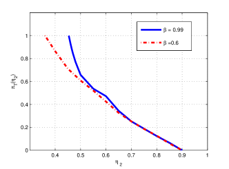
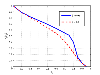
Figure 2: $\pi_{T}(\eta_{2})$ is plotted for $\beta=0.6$ and $\beta=0.99.$ The left plot is for the same set of same parameters as in Fig. 4 whereas the right plot uses $\rho_{0}=\eta_{0}=0.1,$ $\rho_{1}=\eta_{1}=0.95,$ $\mu_{0}=\lambda_{0}=0.9,$ and $\mu_{1}=\lambda_{1}=0.1.$

V Explicit calculation of the Whittle index for the class of threshold policies

Recall Conjecture 1 on a threshold policy for the single-arm hidden Markov bandit. For the cases when the conjecture is true, we can use the definition of the Whittle index for an arm and explicitly evaluate it. The calculations though are tedious and require us to exercise care in enumerating the various cases. This is because the properties of the $\gamma$s in Property 1 depend on the ordering of $\mu$s and $\lambda$s. In the following we will consider, for the sake of an example, one case $\lambda_{0}=\mu_{0}>\mu_{1}=\lambda_{1}.$ The other cases have similar calculations and will be omitted here. We will also continue to assume that $0<\rho_{0}<\rho_{1}<1.$

Figure 3: The different cases to calculate $W(\pi)$ in Section V

For $i=0,1,2,$ define $\gamma_{i}^{(0)}(\pi)=\pi,$ $\gamma_{i}^{(k)}:=\gamma_{i}\left(\gamma_{i}^{(k-1)}(\pi)\right),$ and $\gamma_{i,\infty}:=\lim_{k\rightarrow\infty}\gamma_{i}^{(k)}(\pi).$ We can show that $0<\mu_{1}<\gamma_{1,\infty}<\gamma_{2,\infty}<\gamma_{0,\infty}<\mu_{0}<1.$ See Fig. 3. The interval $(0,1),$ the range of $\pi$ is divided into five regions, denoted $A_{1},\ldots,A_{5},$ as shown in Fig. 3.

1. For $\pi\in A_{1},$ $W(\pi)=\rho(\pi).$

2. For $\pi\in A_{2},$ we will have the following cases

   1. If $\gamma_{1}(\pi)\geq\pi,$ then $W(\pi)=\rho(\pi).$

   2. If $\pi>\gamma_{1}(\pi),$ $\pi\leq\gamma_{0}(\pi),$ $\gamma_{0}(\gamma_{1}(\pi))>\pi,$ and $\gamma_{1}^{(2)}(\pi)\geq\pi$ then

      $$W(\pi)=\frac{(1-\beta)\left[\rho(\pi)+\beta\rho(\pi)\rho(\gamma_{1}(\pi))\right]}{\left(1-\beta\left[1-\rho(\pi)(1-\beta)\right]\right)}.$$

   3. If $\pi>\gamma_{1}(\pi),$ $\pi\leq\gamma_{0}(\pi),$ $\gamma_{0}(\gamma_{1}(\pi))>\pi,$ and $\gamma_{1}^{(2)}(\pi)<\pi,$ then

      $$W(\pi)=\frac{(1-\beta)C_{1}}{[1-(C_{2}+C_{3}+C_{4})]},$$

      where

      $$C_{1} = \sum_{l=0}^{\tau_{1}-1}\beta^{l}\prod_{j=0}^{l}\rho\left(\gamma_{1}^{(j)}(\pi)\right)$$

      $$C_{2} = \beta^{\tau_{1}}\prod_{j=0}^{\tau_{1}-1}\rho\left(\gamma_{1}^{(j)}(\pi)\right)$$

      $$C_{3} = \sum_{l=1}^{\tau_{1}-1}\beta^{l+1}\prod_{j=1}^{l}\rho\left(\gamma_{1}^{(j-1)}(\pi)\right)\left(1-\rho\left(\gamma_{1}^{(l)}(\pi)\right)\right)$$

      $$C_{4} = \beta(1-\rho(\pi))$$

      $$\tau_{1} := \inf\left\{k\geq 1:\gamma_{1}^{(k)}(\pi)\geq\pi\right\}.$$

   4. If $\pi>\gamma_{1}(\pi),$ $\gamma_{0}(\pi)\geq\pi,$ $\gamma_{0}(\gamma_{1}(\pi))<\pi$ and $\gamma_{1}^{(2)}(\pi)<\pi$ then $W(\pi)$ is obtained numerically by performing the value iteration till convergence.

3. For $\pi\in A_{3}$ then the Whittle index is obtained via numerical computation as described above.

4. For $\pi\in A_{4},$ $W(\pi)=\rho(\pi)+\beta\gamma_{2}(\pi)(m-1).$

5. For $\pi\in A_{5},$ then

   $$W(\pi)=m\pi\left(1-\beta(\lambda_{0}-\lambda_{1})\right)+(1-\beta)c-\beta\lambda_{1}m.$$

   where $m=\frac{\rho_{0}-\rho_{1}}{1-\beta(\mu_{0}-\mu_{1})},$ $c=\frac{\rho_{1}+\frac{\beta\mu_{1}(\rho_{0}-\rho_{1})}{1-\beta(\mu_{0}-\mu_{1})}}{1-\beta}.$

We now provide a brief description of the key steps in obtaining the preceding expressions. The key idea is of course to solve $V_{S}(\pi,\eta_{2})=V_{NS}(\pi,\eta_{2})$ for $\eta_{2}.$ This solution is $W(\pi).$ In general, $V_{S}(\pi,\eta_{2})$ and $V_{NS}(\pi,\eta_{2})$ do not have closed form expressions. The key step is to show that for fixed $\eta_{2},$ both $V_{S}(\pi,\eta_{2})$ and $V_{NS}(\pi,\eta_{2})$ have at most three connected components for fixed $\eta_{2}.$ This fact, and the properties of the $\gamma$s are then used to solve for $\eta_{2}.$ For example, for $\pi\in A_{1},$ we have $0\leq\pi\leq\mu_{1},$ $\gamma_{0}(\pi),\gamma_{1}(\pi)\geq\pi$ and $V_{S}(\pi,\eta_{2})=\rho(\pi)+\beta\frac{\eta_{2}}{1-\beta}$ and $V_{NS}(\pi,\eta_{2})=\frac{\eta_{2}}{1-\beta}.$ Equating $V_{S}(\pi,\eta_{2})$ and $V_{NS}(\pi,\eta_{2})$ at $\pi=\pi_{T}$ and solving for $\eta_{2},$ we get $\eta_{2}=\rho(\pi)=W(\pi).$ The other closed form expressions are similarly obtained. For the two cases for which we need to obtain $W(\pi)$ numerically, such a simplification is not possible.

VI Concluding Remarks

Several interesting prospects for future work are open. We would of course like to know for sure if the single armed bandit indeed has a single threshold sampling policy. As we mention in the appendix, the complexity of the $\gamma_{i}$s makes such a proof hard and the ‘usual’ techniques that have been used in the literature do not appear to be useful. The restriction on $\beta$ in the main results are in the same spirit as that of [29]. The approximation is introduced here.

Since we do not have a closed-form expression for $V(\pi)$ and $W(\pi),$ provably good approximations may be sought. Also, since the Whittle index based policy is itself suboptimal, we could seek other suboptimal policies that can provide guarantees on the approximation to optimality.

-A Proof of Lemma  1

Let $x,y\in\Re_{+}^{n}$ and $0\leq\alpha\leq 1.$ Then we have the following.

$$g\left(\alpha x+(1-\alpha)x\right)$$

$$=\ ||\alpha x+(1-\alpha)y||_{1}f\left(\frac{\alpha x+(1-\alpha)y}{||\alpha x+(1-\alpha)y||_{1}}\right)$$

$$=\ ||\alpha x+(1-\alpha)y||_{1}f\left(\frac{\alpha||x||_{1}}{||\alpha x+(1-\alpha)y||_{1}}\frac{x}{||x||_{1}}\right.$$

$$\ \ \ \left.+\frac{(1-\alpha)||y||_{1}}{||\alpha x+(1-\alpha)y||_{1}}\frac{y}{||y||_{1}}\right)$$

$$\leq\ ||\alpha x+(1-\alpha)y||_{1}\left[\frac{\alpha||x||_{1}}{||\alpha x+(1-\alpha)y||_{1}}f\left(\frac{x}{||x||_{1}}\right)\right.$$

$$\ \ \ \left.+\frac{(1-\alpha)||y||_{1}}{||\alpha x+(1-\alpha)y||_{1}}f\left(\frac{y}{||y||_{1}}\right)\right]$$

$$=\ \alpha||x||_{1}f\left(\frac{x}{||x||_{1}}\right)+(1-\alpha)||y||_{1}f\left(\frac{y}{||y||_{1}}\right)$$

$$=\ \alpha g(x)+(1-\alpha)g(y)$$

The inequality in the fifth line follows from convexity of $f.$

-B Proof of Lemma 2

For part (1), we first prove that $V(\pi)$ is convex by induction and use this to show that $V_{S}(\pi)$ and $V_{NS}(\pi)$ are also convex. Let

$$V_{1}(\pi) = \max\left\{\pi\rho_{0}+(1-\pi)\rho_{1},\eta_{2}\right\},$$

$$V_{n+1}(\pi) = \max\left\{\eta_{2}+\beta V_{n}(\gamma_{2}(\pi)),\right.\rho(\pi)+$$ (12)

$$\left.\beta\left[\rho(\pi)V_{n}(\gamma_{1}(\pi))+(1-\rho(\pi))V_{n}(\gamma_{0}(\pi))\right]\right\}.$$

Now define

$$b_{0} := \left[\pi\mu_{0}(1-\rho_{0})+(1-\pi)\mu_{1}(1-\rho_{1}),\right.$$

$$\ \left.(1-\mu_{0})(1-\rho_{0})\pi+(1-\pi((1-\mu_{1})(1-\rho_{1})\right]^{T},$$

$$b_{1} := \left[\pi\mu_{0}\rho_{0}+(1-\pi)\mu_{1}\rho_{1},\right.$$ (13)

$$\left.(1-\mu_{0})\rho_{0}\pi+(1-\pi((1-\mu_{1})\rho_{1}\right]^{T},$$

and write (12) as

$$V_{S,n+1}(\pi) = ||b_{1}||_{1}+\beta||b_{1}||_{1}V_{n}\left(\frac{b_{1}}{||b_{1}||_{1}}\right)+\beta||b_{0}||_{1}V_{n}\left(\frac{b_{0}}{||b_{0}||_{1}}\right).$$

Here superscript $T$ denotes the transpose. Clearly, $V_{1}(\pi)$ is linear and hence convex. Making the induction hypothesis that $V_{n}(\pi)$ is convex in $\pi,$ $V_{S,n+1}(\pi)$ and $V_{n+1}(\pi)$ are convex from Lemma 1 and by induction $V_{n}(\pi)$ is convex for all $n.$ From Chapter 7 of [27] and Proposition 2.1 of Chapter 2 of [28], $V_{n}(\pi)\to V(\pi)$ and hence $V(\pi)$ is convex, Further,

$$V^{\prime\prime}_{NS}(\pi) = \beta V^{\prime\prime}(\gamma_{2}(\pi))\left(\gamma_{2}^{\prime}(\pi)\right)^{2}$$

and hence $V_{NS}$ is also convex. Using the notation from (13), we can write

$$V_{S}(\pi)=||b_{1}||_{1}+\beta||b_{1}||_{1}V\left(\frac{b_{1}}{||a_{1}||b_{1}}\right)+\beta||b_{0}||_{1}V\left(\frac{b_{0}}{||b_{0}||_{1}}\right).$$

The first term in the RHS above is clearly convex in $\pi.$ Since $V(\pi)$ is convex, from Lemma 1, the second and third terms are also convex. Thus $V_{S}(\pi)$ is convex.

To prove the second part of the lemma we rewrite the recursion of (12) as follows.

$$V_{1}(\pi,\eta_{2}) = \max\{\rho(\pi),\eta_{2}\}$$

$$V_{n+1}(\pi,\eta_{2}) = \max\left\{\eta_{2}+\beta V_{n}(\gamma_{2}(\pi),\eta_{2}),\rho(\pi)+\right.$$ (14)

$$\left.\rho(\pi)\beta V_{n}(\gamma_{1}(\pi),\eta_{2})+\left(1-\rho(\pi)\right)\beta V_{n}(\gamma_{0}(\pi),\eta_{2})\right\}$$

Here we have made explicit the dependence of $V(\pi)$ on $\eta_{2}.$ We see that $V_{1}(\pi,\eta_{2})$ is monotone non decreasing and convex in $\eta_{2}.$ Make the induction hypothesis that for a fixed $\pi,$ $V_{n}(\pi,\eta_{2})$ is monotone non decreasing and convex in $\eta_{2}.$ Then, in (14), the first term of the $\max$ function is the sum of two non decreasing convex functions of $\eta_{2}.$ The second term is a constant plus a convex sum of two non decreasing convex functions of $\eta_{2}.$ Thus it is also non decreasing and convex in $\eta_{2}.$ The max operation preserves convexity. Thus $V_{n+1}(\pi,\eta_{2})$ is also non decreasing and convex in $\eta_{2}$ and by induction, all $V_{n}(\pi,\eta_{2})$ are non decreasing and convex in $\eta_{2}.$ As in the first part of the lemma, $V_{n}(\pi,\eta_{2})\to V(\pi,\eta_{2})$ and this completes the proof for $V(\pi).$ From (4), the assertion on $V_{S}(\pi)$ and $V_{NS}(\pi)$ follows.

-C Proof that $V_{\beta}(\pi,\eta_{2})$ is increasing in $\beta$

If $\beta_{a}>\beta_{b},$ we need to show that $V_{\beta_{a}}(\pi,\eta_{2})>V_{\beta_{b}}(\pi,\eta_{2}).$ Like in earlier proofs, we use an induction argument. Let

$$V_{S,\beta,1}(\pi,\eta_{2}) := \rho(\pi),$$

$$V_{NS,\beta,1}(\pi,\eta_{2}) := \eta_{2},$$

$$V_{\beta,1}(\pi,\eta_{2}) := \max\{V_{S,\beta,1}(\pi,\eta_{2}),V_{NS,\beta,1}(\pi,\eta_{2})\},$$

and define

$$V_{S,\beta,n+1}(\pi,\eta_{2}) := \rho(\pi)+\beta\left[\rho(\pi)V_{\beta,n}(\gamma_{1}(\pi),\eta_{2})+\right.$$

$$\hskip 10.0pt\left.(1-\rho(\pi))V_{\beta,n}(\gamma_{0}(\pi),\eta_{2})\right],$$

$$V_{NS,\beta,n+1}(\pi,\eta_{2}) := \eta_{2}+\beta V_{\beta,n}(\gamma_{2}(\pi),\eta_{2}),$$

$$V_{\beta,n+1}(\pi,\eta_{2}) := \max\{V_{S,\beta,n}(\pi,\eta_{2}),V_{NS,\beta,n}(\pi,\eta_{2})\}.$$

Clearly, $V_{S,\beta,1}(\pi,\eta_{2}),$ $V_{NS,\beta,1}(\pi,\eta_{2})$ and $V_{\beta,1}(\pi,\eta_{2})$ are all increasing in $\beta.$

Now make the induction hypothesis that $V_{S,\beta,n}(\pi,\eta_{2}),$ $V_{NS,\beta,n}(\pi,\eta_{2})$ and by inspection of (LABEL:eqn:induction-for-Vbeta) we see that $V_{S,\beta,n+1}(\pi,\eta_{2}),$ $V_{NS,\beta,n+1}(\pi,\eta_{2}),$ and $V_{\beta,n+1}(\pi,\eta_{2})$ are all increasing in $\beta.$ Further, like in the proof Lemma 2, we know that

$$V_{n,S,\beta}(\pi,r_{2}) \rightarrow V_{S,\beta}(\pi,r_{2}),$$

$$V_{n,NS,\beta}(\pi,r_{2}) \rightarrow V_{NS,\beta}(\pi,r_{2}),$$

$$V_{n,\beta}(\pi,r_{2}) \rightarrow V_{\beta}(\pi,r_{2}),$$

and the claim follows.

-D Proof of Lemma 3

For a function $f:\Re\rightarrow\Re$ that is continuous and Lipschitz, we specialize the notion of a generalized gradient (see, e.g., [30]) and define

$$\partial f(x):=\mathsf{co}\{\partial f_{L}(x),\partial f_{R}(x)\}.$$

Here $\partial f_{L}(x)$ and $\partial f_{R}(x)$ are, respectively, the left and right derivatives of $f$ at $x$ and $\mathsf{co}\{\}$ represents the convex hull. Many operations and properties of the gradient follow through to the generalized gradient. In particular, the following will be used.

• (Chain rule) If $f(x)=(g\circ h)(x),$ with $g:\Re\rightarrow\Re$ and $h:\Re\rightarrow\Re,$ $h$ is differentiable and $g$ is convex, then

  $$\partial f(x)=\partial g(h(x))\frac{dh(x)}{dx}.$$

• (Mean value theorem) If $x,y\in\Re,$ $f$ is Lipschitz on an open set containing line segment $[x,y],$ then there exists a point $u\in(x,y)$ such that

  $$f(y)-f(x)\in(y-x)\cdot\partial f(u).$$

First, for any $0\leq\pi_{1}\leq\pi_{2}\leq 1,$ we obtain a bound on $|V(\pi_{2})-V(\pi_{1})|.$ The proof will follow the iterative technique as in Appendix -C. Define $\kappa_{1}:=(1-\beta|\mu_{0}-\mu_{1}|)^{-1}.$

Lemma 5

For a fixed $\eta_{2},$ $\beta_{2}\in(0,1],$ and $0\leq\pi_{1}\leq\pi_{2}\leq 1,$ if either $0<\mu_{0}-\mu_{1}\leq\frac{1}{2}$ or $0<\mu_{1}-\mu_{0}<1$ is true, then

$$\big{|}V(\pi_{2})-V(\pi_{1})\big{|}\leq\kappa_{1}|\rho_{1}-\rho_{0}||\pi_{2}-\pi_{1}|.$$

Proof:

We present the calculations for $0<\mu_{0}-\mu_{1}\leq\frac{1}{2}.$ The calculations for $0<\mu_{1}-\mu_{0}<1$ are identical.

1. Let $V_{1}(\pi)=\max\{\rho(\pi),\eta_{2}\},$ recall that $\rho(\pi)=\pi(\rho_{0}-\rho_{1})+\rho_{1}$ and $\rho_{0}<\rho_{1}.$ The generalized gradient of $V_{1}$ at $\pi\in[0,1]$ is

   $$\partial V_{1}(\pi) = \mathsf{co}\{\rho_{0}-\rho_{1},0\}=[\rho_{0}-\rho_{1},0]$$

   $$\subset [-\kappa_{1}(\rho_{1}-\rho_{0}),\kappa_{1}(\rho_{1}-\rho_{0})].$$

2. Applying the the chain rule on the generalized gradient, we get

   $$\partial V_{S,n+1}(\pi) = \mathrm{co}\bigg{\{}(\rho_{0}-\rho_{1})$$

   $$+\beta(\rho_{1}-\rho_{0})\left[V_{n}(\gamma_{0}(\pi))-V_{n}(\gamma_{1}(\pi))\right]$$

   $$+\beta\frac{\rho_{1}\rho_{0}(\mu_{0}-\mu_{1})}{(\rho(\pi))}\partial V_{n}((\gamma_{1}(\pi)))$$

   $$+\beta\frac{(1-\rho_{1})(1-\rho_{0})(\mu_{0}-\mu_{1})}{(1-\rho(\pi))}\partial V_{n}(\gamma_{0}(\pi))\bigg{\}}$$

3. We make the induction hypothesis that $\big{|}V_{n}(\pi_{2})-V_{n}(\pi_{1})\big{|}\leq\kappa_{1}|\rho_{1}-\rho_{0}||\pi_{2}-\pi_{1}|$ for all $0\leq\pi_{1}\leq\pi_{2}\leq 1$ and provide upper and lower bounds for $\partial V_{S,n+1}(\pi).$

4. First, consider the upper bound. For $\mu_{0}>\mu_{1},$ from Property 1, we see that for $0\leq\pi\leq 1,$ $\mu_{0}>\gamma_{0}(\pi)>\gamma_{1}(\pi)>\mu_{1}.$ Hence $\left(\gamma_{0}(\pi)-\gamma_{1}(\pi)\right)\leq(\mu_{0}-\mu_{1}).$ Using this and the mean value theorem for the generalized gradient, we obtain the following bound.

   $$\big{|}V_{n}(\gamma_{0}(\pi))-V_{n}(\gamma_{1}(\pi))\big{|} \leq \kappa_{1}(\rho_{1}-\rho_{0})(\mu_{0}-\mu_{1}),$$

   Further, from the induction hypothesis,

   $$\partial V_{n}(\gamma_{1}(\pi)),\partial V_{n}(\gamma_{0}(\pi))=[-\kappa_{1}(\rho_{1}-\rho_{0}),\kappa_{1}(\rho_{1}-\rho_{0})]$$

   Hence, using the observation that $\rho_{0}\leq\rho(\pi)\leq\rho_{1},$ and $(1-\rho_{1})\leq(1-\rho(\pi))\leq(1-\rho_{0}),$ with some calculations we can show that $\partial V_{S,n+1}(\pi)$ is upper bounded by

   $$(\rho_{0}-\rho_{1})+\beta\kappa_{1}(\rho_{1}-\rho_{0})^{2}(\mu_{0}-\mu_{1})$$

   $$+\beta\rho_{1}(\mu_{0}-\mu_{1})\kappa_{1}(\rho_{1}-\rho_{0})$$

   $$+\beta(1-\rho_{0})(\mu_{0}-\mu_{1})\kappa_{1}(\rho_{1}-\rho_{0})$$

   which, after rearranging the terms becomes

   $$(\rho_{1}-\rho_{0})\kappa_{1}\left(-1+4\beta(\mu_{0}-\mu_{1})\right).$$ (17)

   Now, since $0<\mu_{0}-\mu_{1}\leq\frac{1}{2},$ we have $(-1+4\beta(\mu_{0}-\mu_{1}))\leq(-1+2\beta)\leq 1,$ and the upper bound becomes $\kappa_{1}(\rho_{1}-\rho_{0})$

5. To obtain the lower bound, we substitute $\rho(\pi)\leq\rho_{1}$ and $(1-\rho(\pi))\leq(1-\rho_{0})$ in Eq.  (LABEL:eq:partial-V-S-pi-nplusa). Using the induction hypothesis on $V_{n}(\pi),$ we can show that the lower bound is $-\kappa_{1}(\rho_{1}-\rho_{0}).$

6. From the preceding two steps we have

   $$\partial V_{S,n+1}(\pi)\subseteq[-\kappa_{1}(\rho_{1}-\rho_{0}),\kappa_{1}(\rho_{1}-\rho_{0})].$$

7. Now consider generalized gradient of $V_{NS,n+1}(\pi)$ w.r.t. $\pi.$ From equation (LABEL:eqn:induction-for-Vbeta), using properties of $\gamma_{2}(\pi)$ and the induction hypothesis on $V_{n}(\pi)$ with some algebra, we can obtain following inequality.

   $$\partial V_{NS,n+1}(\pi)\subseteq[-\kappa_{1}(\rho_{1}-\rho_{0}),\kappa_{1}(\rho_{1}-\rho_{0})].$$

8. From the preceding two steps, we have

   $$\partial V_{n+1}(\pi)\subseteq[-\kappa_{1}(\rho_{1}-\rho_{0}),\kappa_{1}(\rho_{1}-\rho_{0})].$$

   Thus, $\partial V_{n}(\pi)\subseteq[-\kappa_{1}(\rho_{1}-\rho_{0}),\kappa_{1}(\rho_{1}-\rho_{0})]$ holds for every $n\geq 1$ and $\pi\in[0,1].$ Also, $\lim_{n\rightarrow\infty}V_{n}(\pi)=V(\pi)$ converges uniformly. Hence

   $$\partial V(\pi)=[-\kappa_{1}(\rho_{1}-\rho_{0}),\kappa_{1}(\rho_{1}-\rho_{0})].$$

   Our claim follows.

∎

We are now ready to prove Lemma 3. We consider the two cases separately.

Case 1: $0<\mu_{0}-\mu_{1}\leq\frac{1}{5}$ and $|\lambda_{0}-\lambda_{1}|\leq\frac{1}{5}.$ Define

$$d(\pi):=V_{S}(\pi)-V_{NS}(\pi).$$ (18)

The result is proved by showing that $\partial d(\pi)<0.$ Consider

$$\partial d(\pi) = \partial V_{S}(\pi)-\partial V_{NS}(\pi).$$

From the chain rule of the generalized gradient, we obtain

$$\partial V_{NS}(\pi)=\mathrm{co}\bigg{\{}\beta\partial V(\gamma_{2}(\pi))\gamma_{2}^{\prime}(\pi)\bigg{\}}.$$

Further, we can show that $\partial V_{NS}(\pi)$ is lower bounded by $-\beta\kappa_{1}(\rho_{1}-\rho_{0})|\lambda_{0}-\lambda_{1}|$ and $\partial V_{S}(\pi)$ can be upper bounded by

$$(\rho_{1}-\rho_{0})\kappa_{1}(1-\beta(\mu_{0}-\mu_{1})).$$

Thus we can upper bound $\partial d(\pi)$ by

$$(\rho_{1}-\rho_{0})\kappa_{1}\left(-1+4\beta(\mu_{0}-\mu_{1})+\beta|\lambda_{0}-\lambda_{1}|\right).$$

By our assumptions on $(\mu_{0}-\mu_{1})$ and $|\lambda_{0}-\lambda_{1}|,$ The upper bound on $\partial d(\pi)$ is less than $0.$ Hence our claim follows.

Case 2: $0<\mu_{1}-\mu_{0}\leq\frac{1}{3}$ and $|\lambda_{0}-\lambda_{1}|\leq\frac{1}{3}.$ Here, we can obtain following upper bound on $\partial d(\pi)$ using similar tricks.

$$(\rho_{1}-\rho_{0})\kappa_{2}\left\{-1+2\beta(\mu_{1}-\mu_{0})+\beta|\lambda_{0}-\lambda_{1}|\right\}.$$

From our assumptions on $(\mu_{1}-\mu_{0})$ and $|\lambda_{0}-\lambda_{1}|,$ we can show the upper bound on $\partial d(\pi)$ is less than $0.$

This completes the proof.

-E Sample Numerical Results for $V_{S}(\pi)$ and $V_{NS}(\pi)$

We present some numerical results and plot $V_{S}(\pi)$ and $V_{NS}(\pi)$ for different values of $\beta,$ the $\eta_{2}$ $\mu_{i},$ $\lambda_{i},$ and $\rho_{i}.$ The sample plots in Fig. 4 and in many others that we computed indicate that there is only threshold.

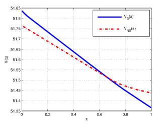
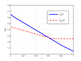
$\beta=0.99;$ $\pi_{T}=0.673.$	$\beta=0.6;\pi_{T}=0.604.$

$\eta_{2}=0.5;$ $\pi^{\circ}=0.5.$

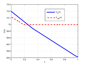
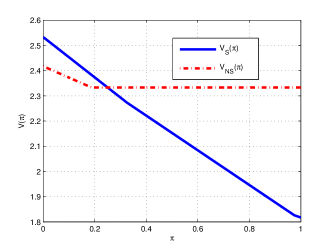
$\beta=0.99;$ $\pi_{T}=0.248.$	$\beta=0.6;$ $\pi_{T}=0.248.$

$\eta_{2}=0.7;$ $\pi^{\circ}=0.25.$

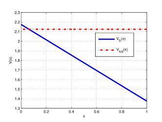
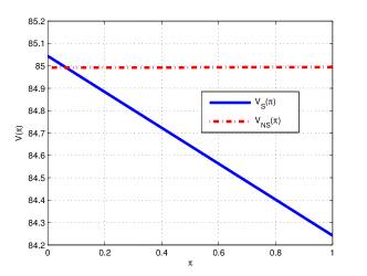
$\beta=0.99$ $\pi_{T}=0.06$	$\beta=0.6;\pi_{T}=0.06.$

$\eta_{2}=0.85;$ $\pi^{\circ}=0.0625.$

Figure 4: $V_{NS}(\pi),$ and $V_{S}(\pi)$ are plotted for different $\eta_{2}$ and $\beta.$ Observe the single threshold in all the cases. The threshold $\pi_{T}$ and the $\pi^{\circ}$ are also indicated for each case. Here we have used $\rho_{0}=\eta_{0}=0.1,$ $\rho_{1}=\eta_{1}=0.9,$ $\mu_{0}=0.1,$ $\mu_{1}=0.9,$ $\lambda_{0}=0.9,$ and $\lambda_{1}=0.1.$

-F Proof of Lemma 4

Proof:

We will establish the contrapositive, i.e., assuming that $\pi_{T}(\eta_{2})$ is not a monotonically decreasing function of $\eta_{2}$ at $\hat{\eta}_{2}$, we will show that

$$\frac{\partial V_{S}(\pi,\eta_{2})}{\partial\eta_{2}}\biggr{\rvert}_{\pi=\pi_{T}(\hat{\eta}_{2})}\geq\frac{\partial V_{NS}(\pi,\eta_{2})}{\partial\eta_{2}}\biggr{\rvert}_{\pi=\pi_{T}(\hat{\eta}_{2})}.$$

Suppose there exists a $\hat{\eta}_{2}\in[\eta_{L},\eta_{H}]$ such that $\pi_{T}(\eta_{2})$ is increasing at $\hat{\eta}_{2}$ i.e., there exists a $c>0,$ such that for all $\epsilon\in[0,c]$

$$\pi_{T}({\hat{\eta}_{2}})\leq\pi_{T}(\hat{\eta}_{2}+\epsilon).$$

This implies that for all $\epsilon\in(0,c)$

$$V_{S}\left(\pi_{T}(\hat{\eta}_{2}),\hat{\eta}_{2}+\epsilon\right)\geq V_{NS}\left(\pi_{T}(\hat{\eta}_{2}),\hat{\eta}_{2}+\epsilon\right).$$ (19)

Further, from the definition of $\pi_{T}(\eta_{2}),$ we also have

$$V_{S}\left(\pi_{T}(\hat{\eta}_{2}),\hat{\eta}_{2}\right)=V_{NS}\left(\pi_{T}(\hat{\eta}_{2}),\hat{\eta}_{2}\right).$$ (20)

Using (19) and (20) we can write the following.

$$V_{S}\left(\pi_{T}(\hat{\eta}_{2}),\hat{\eta}_{2}+\epsilon\right)-V_{S}\left(\pi_{T}(\hat{\eta}_{2}),\hat{\eta}_{2}\right)$$

$$\geq\ V_{NS}\left(\pi_{T}(\hat{\eta}_{2}),\hat{\eta}_{2}+\epsilon\right)-V_{NS}\left(\pi_{T}(\hat{\eta}_{2}),\hat{\eta}_{2}\right).$$

Dividing both sides of the above inequality by $\epsilon,$ taking limits as $\epsilon\to 0,$ and evaluating at $\pi=\pi_{T}(\hat{\eta}_{2})$ gives us

$$\frac{\partial V_{S}(\pi)}{\partial\eta_{2}}\biggr{\rvert}_{\pi=\pi_{T}(\hat{\eta}_{2})}\geq\frac{\partial V_{NS}(\pi)}{\partial\eta_{2}}\biggr{\rvert}_{\pi=\pi_{T}(\hat{\eta}_{2})}.$$

This completes the proof. ∎

-G Numerical Examples

We discussed the difficulties in obtaining closed-form expression for either of $V(\pi),$ $\pi_{T}(\eta_{2}),$ or $W(\pi)$ in some detail in Section -H. A simple solution would be to numerically evaluate and precompute the $W(\pi)$ by suitably discretizing the $(0,1)$ interval. We use this technique and performed several simulation experiments to evaluate the goodness of the Whittle-index policy as compared to a simpler myopic policy that would simply index the arms using $[\pi_{n}(t)\eta_{0}+(1-\pi_{n}(t))\eta_{1}]$ for arm $n.$ This is the expected instantaneous payoff when the arm is sampled in slot $t.$

A sample of the numerical results is presented for the following parameters for a 10-armed bandit.

$$\eta_{0} = [0.1,0.1,0.2,0.4,0.2,0.1,0.3,0.3,0.35,0.05]$$

$$\eta_{1} = [0.9,0.95,0.8,0.9,0.6,0.5,0.95,0.7,0.85,0.5]$$

$$\mu_{0} = [0.1,0.9,0.3,0.9,0.3,0.9,0.3,0.8,0.9,0.5]$$

$$\mu_{1} = [0.9,0.1,0.9,0.3,0.9,0.3,0.9,0.3,0.1,0.02]$$

$$\lambda_{0} = [0.9,0.9,0.1,0.1,0.9,0.9,0.9,0.8,0.9,0.5]$$

$$\lambda_{1} = [0.1,0.1,0.8,0.8,0.4,0.3,0.4,0.3,0.1,0.02].$$

Further, $\rho_{0}=\eta_{0},$ and $\rho_{1}=\eta_{1}.$

In the simulation, the arm with the highest index is chosen to be played in each slot. The simulations start the arms in a random state and a random belief about the state of the arm. In each slot one arms is chosen to be played according to the given policy (Whittle-index based or myopic). The reward obtained in each slot is stored and these rewards are averaged over a $K$ iterations. The data is collected after of 2000 slots.

Fig. 5 plots the instantaneous value of the reward averaged over $K$ iterations for different values of $\beta$ and $K.$ For The Whittle-index policy has a consistently better reward than than the myopic policy although the difference reduces with decreasing $\beta.$ Our extensive simulations indicate similar behaviour for a large set of parameters with the two becoming comparable in a few cases.

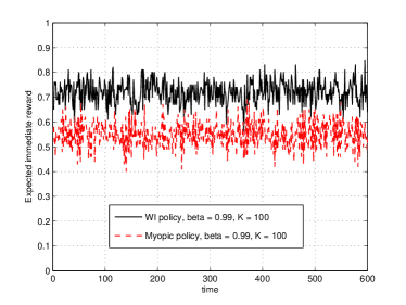
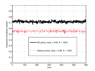
$\beta=0.99,\ K=100$	$\beta=0.99\ K=1000$
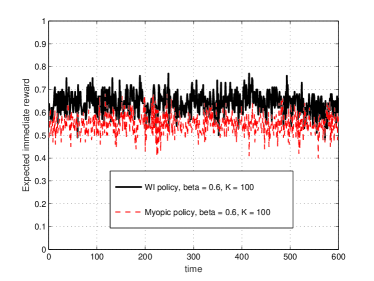
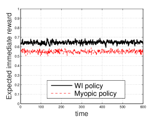
$\beta=0.6,\ K=100$	$\beta=0.6,\ K=1000$
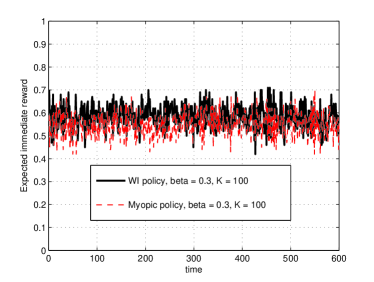
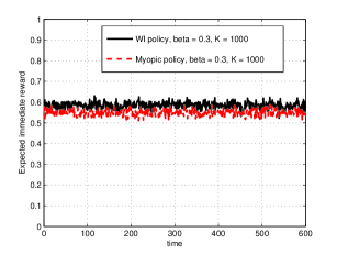
$\beta=0.3,\ K=100$	$\beta=0.3,\ K=1000$

Figure 5: The average instantaneous reward obtained from the Whittle-index based policy for different values of $\beta$ and for the myopic policy. The average reward shown is averaged over 100 and 1000 iterations.

-H Complications due to hidden states

In this paper we are able to provide a structural property through Theorems 1 and 2, but a obtain a closed-form expressions for the value function $V(\pi),$ the threshold $\pi_{T}(\eta_{2}),$ or the Whittle’s index $W(\pi)$ have been elusive. We briefly discuss the complications that the hidden states of the arms that makes it difficult to obtain these quantities as compared to the other extant models.

Most models in the literature assume that when an arm is sampled, its state is correctly observed. In our model, this means that when the arm is sampled, the binary signal could just correspond to the state of the arm and have $\rho_{0}=0$ and $\rho_{1}=1.$ In this case, $\gamma_{0}(\pi)=\mu_{0}$ and $\gamma_{1}(\pi)=\mu_{1}$ both of which are independent of $\pi.$ Compare this with the $\gamma_{i}$s for our model that are non linear functions of $\pi!$ Further, in the models where the state is observed, we will have

$$V_{S}(\pi) = (1-\pi)+\beta(1-\pi)V(\mu_{1})+\beta\pi V(\mu_{0}),$$

$$V_{NS}(\pi) = \eta_{2}+\beta V(\gamma_{2}(\pi)).$$

This means that $V_{S}(\pi)$ can be evaluated by evaluating $V(\pi)$ at two points. Further, the structure of the optimal policy will be to continue to sample while the sampled arm is observed to be in the good state. If the arm is sampled to be in the bad state, then wait till $\pi$ crosses $\pi_{T}$ before sampling again. The number of slots to wait for this is easy to determine if $\pi_{T}$ is known. In our case, if the arm is sampled and a binary $1$ is observed, the new $\pi$ depends on the current value of $\pi$ and a policy like above will not work. A similar argument applies if the arm is sampled and a $0$ is observed.

While obtaining closed-form expressions appears to be hard the following properties of the $\gamma$s, obtained from first and second derivatives, may be useful in obtaining approximations. We will not explore that in this paper.

Property 1

1. If $\lambda_{0}<\lambda_{1}$ then $\gamma_{2}(\pi)$ is linear decreasing in $\pi.$ Further, $\lambda_{0}\leq\gamma_{2}(\pi)\leq\lambda_{1}.$

2. If $\lambda_{0}>\lambda_{1}$ then $\gamma_{2}(\pi)$ is linear increasing in $\pi.$ Further, $\lambda_{1}\leq\gamma_{2}(\pi)\leq\lambda_{0}.$

3. If $\mu_{0}>\mu_{1}$ then $\gamma_{1}(\pi)$ is convex increasing in $\pi.$ Further, $\mu_{1}\leq\gamma_{1}(\pi)\leq\mu_{0}.$

4. If $\mu_{0}>\mu_{1}$ then $\gamma_{0}(\pi)$ is concave increasing in $\pi.$ Further, $\mu_{1}\leq\gamma_{0}(\pi)\leq\mu_{0}.$

5. $\gamma_{0}(0)=\gamma_{1}(0)=\mu_{1}$ and $\gamma_{0}(1)=\gamma_{1}(1)=\mu_{0}.$ Further, if $\mu_{0}>\mu_{1}$ then $\gamma_{1}(\pi)<\gamma_{0}(\pi)$ for $0<\pi<1.$

∎

References

- [1] E. N. Gilbert, “Capacity of a Burst-Noise Channel,” Bell System Technical Journal, vol. 39, no. 5, pp. 1253–1265, 1960.
- [2] C. H. Papadimitriou and J. H. Tsitsiklis, “The complexity of optimal queueing network control,” Mathematics of Operations Research, vol. 24, no. 2, pp. 293–305, May 1999.
- [3] J. Niño-Mora, “An index policy for dynamic fading-channel allocation to heterogeneous mobile users with partial observations,” in Proceedings of the Conference on Next Generation Internet Networks, April 2008, pp. 231–238.
- [4] J. Niño-Mora, “A restless bandit marginal productivity index for opportunistic spectrum access with sensing errors,” in Proceedings of Conference on Network Control Optimization (NET-COOP), LNCS 5894, 2009, pp. 60–74.
- [5] K. Liu and Q. Zhao, “Indexability of restless bandit problems and optimality of Whittle index for dynamic multichannel access,” IEEE Transactions Information Theory, vol. 56, no. 11, pp. 5557–5567, November 2010.
- [6] C. Lott and D. Teneketzis, “On the optimality of the index rule in multichannel allocation for single-hop mobile networks with multiple service classes,” Probability in the Engineering and Information Sciences, vol. 14, pp. 259–297, 2010.
- [7] Q. Zhao, B. Krishnamachari, and K. Liu, “On myopic sensing for multi-channel opportunistic access: structure, optimality, and performance,” IEEE Transactions on Wireless Communication, vol. 7, no. 12, pp. 5431–5440, December 2008.
- [8] K. Wang, L. Chen, and Q. Liu, “On optimality of myopic sensing policy with imperfect sensing in multi-channel opportunistic access,” IEEE Transactions on Communications, vol. 61, no. 9, pp. 3854–3862, September 2013.
- [9] K. Wang, L. Chen, and Q. Liu, “On optimality of myopic policy for opportunistic access with nonidentical channels and imperfect sensing,” IEEE Transactions on Vehicular Technology, vol. 63, no. 5, pp. 2478–2483, June 2014.
- [10] W. Ouyang, A. Eyrilmaz, and N. Shroff, “Asymptotically optimal downlink scheduling over Markovian fading channels,” in Proceedings of IEEE INFOCOM, 2012, pp. 1224–1232.
- [11] Q. Zhao, L. Tong, A. Swami, and Y. Chen, “Decentralized cognitive MAC for opportunistic spectrum access in ad hoc networks: A POMDP framework,” IEEE Journal on Selected Areas in Communications, vol. 25, no. 3, pp. 589–600, April 2007.
- [12] Y. Chen, Q. Zhao, and A. Swami, “Joint design and separation principle for opportunistic spectrum access in the presence of sensing errors,” IEEE Transactions on Information Theory, vol. 54, no. 5, pp. 2053–2071, May 2008.
- [13] C. Li and M. J. Neely, “Network utility maximization over partially observable Markovian channels,” Performance Evaluation, vol. 70, no. 7–8, pp. 528–548, July 2013.
- [14] P. Whittle, “Restless bandits: Activity allocation in a changing world,” Journal of Applied Probability, vol. 25, no. A, pp. 287–298, 1988.
- [15] M. H. Veatch and L. M. Wein, “Scheduling a make-to-stock queue: Index policies and hedging points,” Operations Research, vol. 44, no. 4, pp. 634–647, July-August 1996.
- [16] J. L. Ny, M. Dahleh, and E. Feron, “Multi-UAV dynamic routing with partial observations using restless bandit allocation indices,” in Proceedings of American Control Conference (ACC), 2008, pp. 4220–4225.
- [17] W. Ouyang, S. Murugesan, A. Eyrilmaz, and N. Shroff, “Exploiting channel memory for joint estimation and scheduling in downlink networks,” in Proceedings of IEEE INFOCOM, 2011.
- [18] K. Avrachenkov, U. Ayesta, J. Doncel, and P. Jacko, “Congestion control of TCP flows in Internet routers by means of index policy,” Computer Networks, vol. 57, no. 17, pp. 3463–3478, 2013.
- [19] K. Avrachenkov and V. S. Borkar, “Whittle index policy for crawling ephemeral content,” IEEE Transactions on Control of Network Systems, 2016, DOI:10.1109/TCNS.2016.2619066.
- [20] J. E. Niño-Mora, “Restless bandits, partial conservation laws and indexability,” Advances in Applied Probability, vol. 33, pp. 76–98, 2001.
- [21] S. M. Ross, “Quality control under Markovian deterioration,” Management Science, vol. 17, no. 9, pp. 587–596, May 1971.
- [22] E. L. Sernik and S. I. Marcus, “On the computation of optimal cost function for discrete time Markov models with partial observations,” Annals of Operations Research, vol. 29, pp. 471–512, 1991.
- [23] E. L. Sernik and S. I. Marcus, “Optimal cost and policy for a Markovian replacement problem,” Journal of Optimization Theory and Applications, vol. 71, no. 1, pp. 403–406, October 1991.
- [24] J. S. Hughes, “A note on quality control under Markovian deterioration,” Operations Research, vol. 28, no. 2, pp. 421–424, March-April 1980.
- [25] V. Krishnamurthy and R. J. Evans, “Hidden Markov model for multiarm bandits: a methodology for beam scheduling in multitarget tracking,” IEEE Transactions on Signal Processing, vol. 49, no. 12, pp. 2893–2908, December 2001.
- [26] K. J. Astrom, “Optimal control of Markov processes with incomplete state information II. The convexity of loss function,” Mathematical Analysis and Applications, vol. 26, no. 2, pp. 403–406, May 1969.
- [27] D. P. Bertsekas, Dynamic Programming and Optimal Control, vol. 1, Athena Scientific, Belmont, Massachusetts, 1st edition, 1995.
- [28] D. P. Bertsekas, Dynamic Programming and Optimal Control, vol. 2nd, Athena Scientific, Belmont, Massachusetts, 1st edition, 1995.
- [29] C. C. White III, “Optimal control-limit strategies for a partially observed replacement problem,” International Journal of System Science, vol. 10, no. 3, pp. 321–331, 1979.
- [30] F. H. Clarke, Optimization and Nonsmooth Analysis, SIAM, Philadelphia, 1990.