Dense cloud cores revealed by CO in the low metallicity dwarf galaxy WLM

Abstract

Understanding stellar birth requires observations of the clouds in which they form. These clouds are dense and self-gravitating, and in all existing observations, they are molecular with H₂ the dominant species and CO the best available tracer[1, 2]. When the abundances of carbon and oxygen are low compared to hydrogen, and the opacity from dust is also low, as in primeval galaxies and local dwarf irregular galaxies[3], CO forms slowly and is easily destroyed, so it is difficult for it to accumulate inside dense clouds[4]. Here we report interferometric observations of CO clouds in the local group dwarf irregular galaxy Wolf-Lundmark-Melotte (WLM)[5], which has a metallicity that is 13% of the solar value[6, 7] and 50% lower than the previous CO detection threshold. The clouds are tiny compared to the surrounding atomic and H₂ envelopes, but they have typical densities and column densities for CO clouds in the Milky Way. The normal CO density explains why star clusters forming in dwarf irregulars have similar densities to star clusters in giant spiral galaxies. The low cloud masses suggest that these clusters will also be low mass, unless some galaxy-scale compression occurs, such as an impact from a cosmic cloud or other galaxy. If the massive metal-poor globular clusters in the halo of the Milky Way formed in dwarf galaxies, as is commonly believed, then they were probably triggered by such an impact.

Departamento de Astronomía, Universidad de Chile, Casilla 36-D, Santiago, Chile

IBM Research Division, T.J. Watson Research Center, 1101 Kitchawan Road, Yorktown Heights, NY 10598, USA

Lowell Observatory, 1400 West Mars Hill Road, Flagstaff, Arizona 86001 USA

Centre for Astrophysics Research, University of Hertfordshire, Hatfield AL10 9AB, UK

Joint ALMA Observatory, Alonso de Córdova 3107, Vitacura, Santiago, Chile

National Radio Astronomy Observatory Avenida Nueva Costanera 4091, Vitacura, Santiago, Chile

New Mexico Institute of Mining and Technology, Socorro, NM 87801, USA

WLM is an isolated dwarf galaxy at a distance of $985\pm 33$ kpc[5]. Like other dwarfs, the relative abundance of supernova-processed elements (“metals”) like Carbon and Oxygen is low[6], $12+\log(O/H)=7.8$, compared to $8.66$ for the Milky Way[7]. Low C and O abundances, along with the correspondingly low abundances of other processed elements and dust, make the CO molecule rare compared to H₂, and this calls into question the standard model of star formation in CO-rich clouds[1]. In fact, the star formation rate[8] compared to the existing stellar mass is actually high in WLM: 0.006 $M_{\odot}$ yr^-1 of new stars for a total stellar mass[9] of $1.6\times 10^{7}$ $M_{\odot}$ is 12 times higher than in the Milky Way, where the star formation rate[10] is $\sim 1.9\pm 0.4\;M_{\odot}$ yr^-1 and the stellar mass is $6.4\pm 0.6\times 10^{10}\;M_{\odot}$[11]. Thus WLM forms stars efficiently even with a relatively low abundance of CO.

To understand star formation in metal-poor galaxies, which include the most numerous galaxies in the local universe, the dwarfs, plus all primeaval galaxies, we previously searched for CO(3-2) in WLM using the APEX telescope [12], discovering it in two unresolved regions at an abundance relative to H₂ that was half that in the next-lowest metallicity galaxy, the Small Magellanic Cloud. Now, with the completion of the new millimeter and sub-mm wavelength interferometer Atacama Large Millimeter Array (ALMA), we have imaged these two regions in CO(1-0) and resolved the actual molecular structure.

The ALMA maps with $6.2\times 4.3$ pc spatial resolution (HPBW), 5 mJy sensitivity, and 0.5 km s^-1 velocity resolution (FWHM) contain 10 CO clouds with an average radius of 2 parsecs and an average virial mass of $2\times 10^{3}\;M_{\odot}$. Figure 1 shows the CO emission with black contours superposed on HI in green and H$\alpha$ in red. The insert shows a color composite of the optical image in green (V-band), the FUV GALEX image in blue and the HI in red. A [CII]$\lambda$158 $\mu$m image from the Herschel Space Observatory[13] is superposed on the Southeast region in blue[14]. The [CII] is from a photodissociation region including ionized carbon; it is 5 times larger in size than the CO core, indicating a gradual transition between low density atomic gas to high density molecular gas.

Figure 2 shows the contours and spectra of each cloud. The spectral signal-to-noise averages 10 when smoothed to the typical linewidth of 2 km s^-1. Velocities for HI emission are indicated by a bar below each CO spectrum. The cloud properties are summarized in Table 1. The radii $R$ range from 1.5 to 6 pc, obtained using the equation $R=(A/\pi)^{0.5}$ for area $A$, with $A$ determined after deconvolution by quadratic difference with the beam area. The sum of all the line emission measured by ALMA is within a factor of 2 of the total emission found at $18^{\prime\prime}$ resolution by the APEX telescope. The linewidths were corrected for instrumental spectral broadening.

Virial masses for the CO clouds were calculated from the relation $M_{\rm vir}(M_{\odot})=1044R\sigma^{2}$ for $R$ in pc and Gaussian linewidths $\sigma$ in km s^-1. The CO luminosity in K km s^-1 pc² was calculated from $L_{CO}=2453S_{CO}\Delta VD^{2}$ for integrated emission $S$ in Jy km s^-1, FWHM of the line $\Delta V$ in km s^-1, and distance $D$ in Mpc. Figure 3 shows the relationships between these values including other dwarf galaxies (all for CO(1-0)). The CO clouds in WLM satisfy the usual correlations although they are the smallest seen for any of these galaxies. Higher resolution observations should reveal small clouds and/or cores in other galaxies too, but the main point is that WLM has no CO clouds as large as those seen elsewhere.

The virial mass gives some perspective on the conversion from CO luminosity to mass derived previously[12], which was $\alpha_{\rm CO}\sim 124\pm 60\;M_{\odot}\;{\rm pc}^{-2}\left(\rm{K\;km\;s}^{-1}\right)^{-1}$ for the NW region. This value for $\alpha$ was derived from the dust-derived H₂ column density. If instead we take the virial masses and CO luminosities in Table 1, we find that the mean ratio is $\alpha_{\rm vir}\sim 28\pm 28\;M_{\odot}\;{\rm pc}^{-2}\left(\rm{K\;km\;s}^{-1}\right)^{-1}$. If the clouds are not gravitationally bound, then $\alpha_{\rm vir}$ would be smaller. The difference between these two $\alpha$ values arises because most of the H₂ volume has no CO emission, which apparently exists only in the densest cores of the H₂ clouds. For the Milky Way, CO and H₂ have about the same extent in star-forming clouds, making $\alpha_{\rm CO}\sim 4\;M_{\odot}\;{\rm pc}^{-2}\left(\rm{K\;km\;s}^{-1}\right)^{-1}$. When CO does not fill an H₂ cloud, $\alpha$ can be small for each CO core but large for the total H₂ cloud. If the purpose of $\alpha$ is to determine the total H₂ mass in a region based on $L_{\rm CO}$, then the large value should be used.

The self-gravitational boundedness of the CO clouds can be estimated from the general requirement of an associated H₂ density of $\sim 10^{3}$ cm^-3 for collisional excitation[15]. In fact, the virial density of the CO clouds is comparable to this, $n(H_{2})=4.1\times 10^{-21}$ g cm^-3 ($\sim 10^{3}$ cm^-3), from the ratio of the virial mass ($\sim 2\times 10^{3}\;M_{\odot}$) to the cloud volume ($4\pi R^{3}/3$ for $R\sim 2$ pc). Thus the clouds could be marginally bound.

Another measure of CO density is from pressure equilibrium between the CO regions and the weight of the overlying HI and H₂ layers. The H₂ mass column density, $\Sigma_{\rm H2}$, comes from the difference between the total gas column density derived from the dust emission and the HI column density observed at 21 cm. For the NW region[12], $\Sigma_{\rm H2}=31\pm 15\;M_{\odot}$ pc^-2. Adding the HI column density[12] gives $\Sigma_{\rm total}=58\pm 15\;M_{\odot}$ pc^-2. The corresponding pressure from self-gravity is $(\pi/2)G\Sigma_{\rm total}^{2}\sim 1.6\times 10^{-11}$ dynes. Considering the typical CO velocity dispersion for our clouds of $\sigma\sim 0.9$ km s^-1, the ratio of the core pressure to the square of the CO velocity dispersion is the equilibrium core density, $1.9\times 10^{-21}$ g cm^-3, corresponding to $500$ H₂ cm^-3. Thus the virial density, excitation density, and pressure equilibrium density are all about $10^{3}$ cm^-3.

A condition for molecules in the Milky Way is a threshold extinction of $A_{\rm V}=0.3$ mag for H₂ and $\sim 1.5$ mag for CO[16]. These correspond to mass column densities of $6.1\;M_{\odot}$ pc^-2 and $30.3\;M_{\odot}$ pc^-2 in the solar neighborhood. In WLM where the metallicity is 13% solar, the mass thresholds are $47\;M_{\odot}$ pc^-2 and $230\;M_{\odot}$ pc^-2 for the same extinctions, respectively. The first is satisfied by the HI+H₂ envelope of the CO cores ($\sim 58\;M_{\odot}$ pc^-2) and the second is satisfied by the total column density of $220\;M_{\odot}$ pc^-2 calculated from the HI and H₂ envelope, plus the H₂ from the embedded CO core itself (as determined from the CO virial mass, $2\times 10^{3}\;M_{\odot}$, and ALMA measured radius, $2$ pc). These results suggest that the CO clouds in WLM are normal in terms of density, pressure, and column density, which explains why they lie on the standard correlations in Figure 3. They also appear to be marginally self-bound by gravity, suggesting they are related to star formation. Their properties are typical for parsec-size molecular cloud cores in the solar neighborhood[17].

Our observation explains why star clusters have about the same central densities in dwarf irregular[18] and spiral galaxies[19] even though the ambient gas density in dwarfs is much less than in spirals[20]. If the unifying process for star formation is the need to form CO and other asymmetric molecules for cooling (however, see[16, 21]), then the similarity between the CO cores in the two cases accounts for the uniformity of clusters. The small mass of the CO cores in WLM also explains why most dwarf galaxies do not form high mass clusters[18]. The CO parts of interstellar clouds are smaller at lower metallicities, so the clusters that result are smaller too. For example, there are no massive young clusters in these regions of WLM[18]. This lack of massive clusters is usually attributed to sparse sampling of the cluster mass distribution function at low star formation rates[18], but the present observations suggest it could result from some physical reason too, like the lack of massive CO clouds at low metallicity.

When the local dwarf galaxies NGC 1569 and NGC 5253 formed massive clusters, there was a major impact event to increase the pressure and mass at high density[22, 23]. Such an impact would also seem to be needed for the formation of old halo globular clusters, which are massive and low metallicity like their former dwarf galaxy hosts[24, 25].

We wish to thank Phil Massey and the Local Group Survey team for the use of their H$\alpha$ image of WLM. Ms. Lauren Hill made the color composite insert in Figure 1. MR would like to thank Cynthia Herrera (NAOJ) and Jorge Garcia (JAO, ALMA) for support with the CASA implementation to reduce the raw data and A. Rojas for support in the ALMA data reduction. MR is grateful to A. Leroy for providing the galaxy data to produce Figure 3. MR thanks the ALMA Director for the invitation to spend her 2015 sabbatical leave at the Joint ALMA Observatory (JAO) in Santiago, where this article was finished. PC is grateful to Lisa Young and Suzanne Madden for invaluable guidance on Herschel data reduction. MR wishes to acknowledge support from CONICYT (CHILE) through FONDECYT grant No. 1140839. MR is partially supported by CONICYT project BASAL PFB-06. The contributions from DAH were funded by the Lowell Observatory Research Fund. PC acknowledges support from NASA JPL RSA grant 1433776 to Lisa Young and grant 1456896 to DAH. ALMA is a partnership of ESO (representing its member states), NSF (USA) and NINS (Japan), together with NRC (Canada) and NSC and ASIAA (Taiwan), in cooperation with the Republic of Chile. The Joint ALMA Observatory is operated by ESO, AUI/NRAO and NAOJ. The National Radio Astronomy Observatory is a facility of the National Science Foundation operated under cooperative agreement by Associated Universities, Inc.

DAH, Principle Investigator of the ALMA proposal, identified likely CO sources from the re-processed data files using a direct search for significant emission in each frequency channel and for continuous emissions in adjacent channels. MR re-processed the ALMA results from the originally calibrated data delivered by ALMA to get better sensitivity and resolution, finalized the identification of emission sources, extracted spectra of the sources, produced Figures 1 and 2, and produced the measurements in Table 1. BGE wrote the text of the manuscript and interpreted the main science results. EB oversaw the technical application of radio interferometry to molecular line mapping, and determined the noise limitations and deconvolution strategy for the angular size and velocity width measurements. JRC made the size and line-width measurements, produced the virial masses and CO luminosities, determined the main observational parameters and made Figure 3. PC reduced the Herschel [CII] data and made the [CII] map used in Figure 1. All authors contributed to the discussions leading to this manuscript.

This paper makes use of the following ALMA data: ADS/JAO.ALMA#2012.1.00208.S. Reprints and permissions information is available at www.nature.com/reprints. The authors have no competing financial interest in the work described. Correspondence and requests for materials should be addressed to: bge@us.ibm.com.

Table 1: Properties of WLM CO clouds

Region	RA	Dec	Pk Inten	$V_{\rm LSR}$	Flux Den.	Radius	$\sigma$	$M_{\rm vir}$	$L_{\rm CO}$
			(mJy)	(km s-1)	(Jy km s-1)	(pc)	(km s-1)	(M⊙)	(K km s-1 pc2)
NW-1	00 01 57.162	-15 27 00.00	12.2	$-131.79\pm 0.19$	$0.0368\pm 0.0038$	$2.21\pm 1.11$	$1.05\pm 0.17$	$2548\pm 1522$	$81.47\pm 8.39$
NW-2	00 01 57.291	-15 26 52.80	16.1	$-136.42\pm 0.18$	$0.0254\pm 0.0026$	$1.49\pm 0.77$	$0.84\pm 0.28$	$1087\pm 919$	$56.23\pm 5.69$
NW-3	00 01 57.901	-15 26 58.00	10.8	$-126.27\pm 0.15$	$0.048\pm 0.0048$	$2.69\pm 1.35$	$0.75\pm 0.14$	$1561\pm 985$	$106.26\pm 10.71$
NW-4	00 01 58.079	-15 27 00.12	12.2	$-125.38\pm 0.16$	$0.0248\pm 0.0026$	$2.69\pm 1.35$	$0.57\pm 0.14$	$898.4\pm 637$	$54.90\pm 5.84$
SE-1	00 02 01.485	-15 27 42.65	10.8	$-121.85\pm 0.18$	$0.0513\pm 0.0022$	$1.68\pm 0.87$	$0.77\pm 0.18$	$1037\pm 720$	$113.57\pm 11.46$
SE-2	00 02 01.761	-15 27 55.83	13.3	$-118.18\pm 0.16$	$0.0212\pm 0.0023$	$<1$	$0.61\pm 0.23$	$<390\pm 300$	$46.93\pm 5.02$
SE-3	00 02 01.801	-15 27 51.78	14.3	$-120.00\pm 0.12$	$0.0304\pm 0.0031$	$2.21\pm 1.15$	$0.69\pm 0.09$	$1113\pm 653$	$67.30\pm 6.96$
SE-4	00 02 01.864	-15 28 00.52	8.77	$-118.01\pm 0.17$	$0.258\pm 0.0026$	$6.01\pm 1.20$	$1.32\pm 0.14$	$10881\pm 3209$	$571.17\pm 57.20$
SE-5	00 02 02.101	-15 27 58.23	6.92	$-117.21\pm 0.48$	$0.0304\pm 0.0032$	$2.02\pm 0.96$	$1.81\pm 0.57$	$6896\pm 5426$	$67.30\pm 7.16$
SE-6	00 02 02.222	-15 27 52.08	13.7	$-117.79\pm 0.12$	$0.0311\pm 0.0032$	$3.37\pm 1.06$	$0.63\pm 0.15$	$1383\pm 805$	$68.85\pm 7.11$

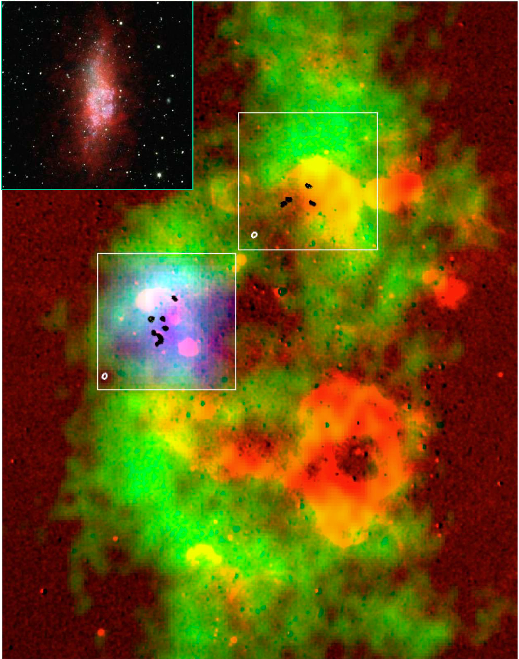
Figure 1: Tiny CO clouds in WLM. A color composite of the various gas phases in WLM: green is the HI [26], red is H$\alpha$[27], and blue is [CII]$\lambda$158 $\mu$m[14]. The CO emission is shown as black single contours inside the 1 arcmin x 1 arcmin white squares that outline the area mapped in ¹²CO (1-0) by ALMA. The synthesized ALMA beam (0.9”x1.3”) is shown in the lower left corner of each square. The inset in the upper left is the full view of WLM obtained by combining HI and optical data: red is HI, green is $V$-band, and blue is GALEX FUV[26]

.

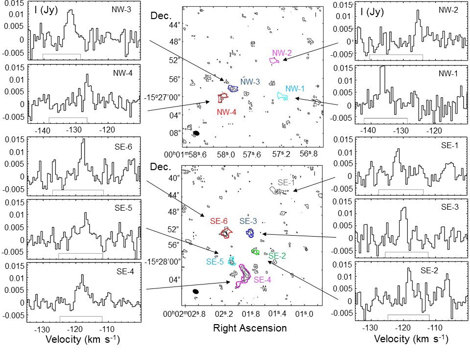
Figure 2: CO clouds and spectra. CO contour maps of the integrated emission starting at the $2-\sigma$ level (RA and DEC in J2000.0 coordinates) . Different CO clouds are identified by color. The ALMA beam is the black ellipse in the lower left corner. The CO spectrum corresponding to each detection is plotted. The velocity for HI emission (FWHM) is shown as a rectangular box on the abscissa (Local Standard of Rest); the CO velocities agree with the HI.

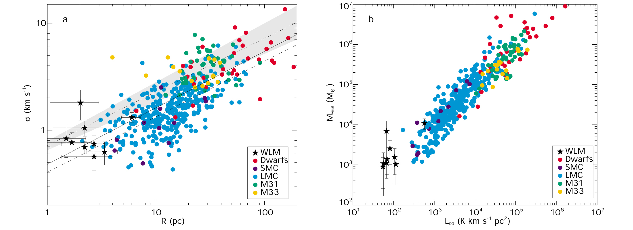
Figure 3: Correlations for CO clouds in dwarf galaxies. The symbols refer to different galaxies (SMC, Dwarfs, M31, and M33[28]; LMC[29]). (a) CO line width $\sigma$ versus radius $R$; the solid line is a fit to WLM, the SMC and dwarf galaxies: $\sigma({\rm km}\;{\rm s}^{-1})=(0.48\pm 0.08)R({\rm pc})^{0.53\pm 0.05}$ and the dashed line includes also the LMC: $\sigma({\rm km}\;{\rm s}^{-1})=(0.40\pm 0.03)R({\rm pc})^{0.52\pm 0.03}$. The black short-dashed line and the gray area indicate the standard relation for the Milky Way[30]: $\sigma=(0.72\pm 0.07)R^{0.50\pm 0.05}$. $R$ for WLM is measured in the same way as for the Milky Way and other galaxies. (b) virial mass versus CO luminosity.

METHODS

0.1 ALMA Observations

We observed the ¹²CO$(J=1-0)$ transition in two regions in WLM using the Atacama Large Millimeter/submillimeter Array (ALMA) located on the Chajnantor Plateau in northern Chile during Cycle 1. Observations were carried out on 2013 July 8 and 2014 April 3. The ALMA receivers were tuned to the ground rotational transition of Carbon Monoxide, CO(1-0). The interferometer configuration C32-2/C32-3 provides a maximum baseline of 0.442 km. The observations were done with a spectral resolution of 122 kHz per channel (0.32 km s^-1) and total bandwidth of 468.750 MHz per baseband. The source J2258–2758 was used as a bandpass calibrator and J2357–1125 was used to calibrate amplitude and phases with time. To set the absolute flux scale, Uranus was observed. We estimated an uncertainty in absolute calibration of 10%.

The data were calibrated, mapped, and cleaned using the ALMA reduction software CASA (version 4.2.1). Rather than use the pipeline-delivered science data cubes, we redid the cleaning (i.e., Fourier transform and beam deconvolution) using a better definition for masking of regions containing emission, and natural weighting to optimize sensitivity. The maximum angular scale for recovered emission was estimated to be 15”.

0.2 Identifying sources

To make a first cut at identifying sources, we convolved the image cube to a 1.25” $\times$1.25” beam and examined a wide velocity range around the velocity expected from the APEX detection. For the SE region we expected signal around $V_{\rm LSR}=-120.5$ km s^-1 and examined $-130.5$ to $-110.5$ km s^-1. We detected candidate sources at $-123$ to $-115.5$ km s^-1. For the NW region we expected signal around $-130.5$ km s^-1 and examined $-140.5$ to $-120.5$ km s^-1, detecting potential sources at $-139$ to $-121.5$ km s^-1. In each velocity channel we looked for knots that had more counts than the majority of knots that were noise. Then we looked for signal in nearly the same location in successive channels, expecting coherence over at least three channels due to the Hanning-smoothing that had been applied. We also generally expected the signal to build up and fade away as the channels sampled the source spectrum. With these criteria, we rated the confidence level of each candidate source as “confident”, “certain”, “not so certain”, or “uncertain”. For the SE region, we identified 9 candidate sources, 6 ranked as “confident” or “certain”. In the NW region, we identified 20 potential sources, 4 ranked as “certain” and the rest as less certain.

Based on this identification, we integrated the emission in the velocity range where CO was seen, and produced the two velocity integrated maps shown in Figure 2 using our reduced new higher sensitivity and velocity resolution cubes. The velocity resolution of these cubes is 0.5 km s^-1 per channel. All velocities are in the Local Standard of Rest (LSR) system. For WLM-SE, 5 integrated maps were made covering a total LSR velocity range $V_{\rm LSR}=-121$ to $-115.5$ km s^-1; the maps spanned velocities of $-121.0$ to $-115.5$, $-121.5$ to $-119.0$, $-119.0$ to $-117.5$, $-118.5$ to $-117.0$, and $-124.0$ to $-120.5$ km s^-1. For WLM-NW, 4 integrated maps were made covering $V_{\rm LSR}=-136.5$ to $-124$ km s^-1; the individual ranges were $-137.0$ to $-135.5$, $-133.5$ to $-130.0$, $-127.5$ to $-125.5$, and $-127.0$ to $-125.5$ km s^-1. For those sources which showed emission at a $3\sigma$ level or above, a spectrum was obtained integrating over an area delineated by a contour drawn at $2\sigma$ (see Figure 2) in order not to miss any genuine emission. We also produced velocity–RA and velocity–Dec maps. Inspecting the CO spectra and the velocity–position maps, we confirmed 10 CO clouds of the original 20 candidates. The remaining 10 were deemed of too low signal-to-noise to be included in this study. On each CO spectrum plot we included the HI emission FWHM velocity width and converted the HI Heliocentric to LSR velocity using $V_{\mathrm{LSR}}$ (i.e. $V_{\mathrm{LSR}}=V_{\mathrm{Helio}}-2.5$ km s^-1).

The total flux of the 10 clouds resolved with ALMA was compared to the CO(3-2) flux in our previous APEX observations. We converted the CO(3-2) APEX fluxes from K km s^-1 to Jy and assumed a thermal CO(1-0)/ CO(3-2) line ratio of 1. For WLM-SE we recovered a similar flux of 0.42 Jy in both cases. For WLM-NW we measured an ALMA flux of 0.14 Jy while the APEX flux converted to CO(1-0) is 0.66 Jy. The difference in the NW can be due to a different line ratio and thus different physical conditions, or it could be from weaker emission not included in our criteria for defining CO clouds, or it could be from emission that is larger in angular extent than the largest structures measured by the interferometer and therefore absent from our maps. If we take both regions, then the measured flux with ALMA is a factor of 2 within the measured flux with APEX.

References

- [1] McKee, C.F., & Ostriker, E.C. “Theory of Star Formation.” Annu. Rev. Astron. Astrophys., 45, 565-687 (2007).
- [2] Kennicutt, R.C., & Evans, N.J. “Star Formation in the Milky Way and Nearby Galaxies.” Annu. Rev. Astron. Astrophys., 50, 531-608 (2012).
- [3] Rémy-Ruyer, A., et al. “Revealing the cold dust in low-metallicity environments. I. Photometry analysis of the Dwarf Galaxy Survey with Herschel,” Astron. Astrophys., 557, A95 (2013).
- [4] Beuther, H. “Carbon in different phases ([CII], [CI], and CO) in infrared dark clouds: Cloud formation signatures and carbon gas fractions.” Astron. Astrophys., 571, A53 (2014).
- [5] Leaman, R., et al. “The resolved structure and dynamics of an isolated dwarf galaxy: a VLT and Keck spectroscopic survey of WLM2012.” Astrophys. J., 750, 33, 20 (2012).
- [6] Lee, H., Skillman, E. D., & Venn, K. A. “Investigating the possible anomaly between nebular and stellar oxygen abundances in the dwarf irregular galaxy WLM.” Astrophys. J., 620, 223–237 (2005)
- [7] Asplund, M. et al. “The Chemical Composition of the Sun” Annu. Rev. Astron. Astophys., 47, 481-522 (2009)
- [8] Hunter, D. A., Elmegreen, B. G., & Ludka, B. C. “GALEX ultraviolet imaging of dwarf galaxies and star formation rates.” Astron. J., 139, 447–475 (2010)
- [9] Zhang, H.-X., Hunter, D. A., Elmegreen, B. G., Gao, Y., & Schruba, A. “Outside-in shrinking of the star-forming disks of dwarf irregular galaxies.” Astron. J., 143, 47, 27 (2012)
- [10] Chomiuk, L., Povich, M.S. “Toward a unification of star formation rate determinations in the Milky Way and other galaxies.” Astron. J., 142, 197, 16 (2011)
- [11] McMillan, P.J. “Mass models of the Milky Way.” Mon. Not. R. Astron. Soc., 414, 2446–2457 (2011)
- [12] Elmegreen, B.G., et al. “Carbon monoxide in clouds at low metallicity in the dwarf irregular galaxy WLM.” Nature, 495, 487-489 (2013).
- [13] Pilbratt et al. “Herschel Space Observatory. An ESA facility for far-infrared and submillimetre astronomy.” Astron. & Astrophys., 518, L1 (2010).
- [14] Cigan, P. et al. “Herschel spectroscopic observations of LITTLE THINGS dwarf galaxies.” Astron.J., submitted, (2015).
- [15] Glover, S.C.O., & Clark, P.C. “Approximations for modelling CO chemistry in giant molecular clouds: a comparison of approaches.” Mon. Not. R. Astron. Soc., 421, 116–131 (2012)
- [16] Glover, S.C.O. & Clark, P.C. “Is molecular gas necessary for star formation?” Mon. Not. R. Astron. Soc., 421, 9–19 (2012)
- [17] Heyer, M. et al. “Re-examining Larsons Scaling Relationships in Galactic Molecular Clouds” Astrophys. J., 699, 1092–1103, (2009).
- [18] Billett, O. H., Hunter, D. A., Elmegreen, B. G. “Compact Star Clusters in Nearby Dwarf Irregular Galaxies.” Astron. J., 123, 1454-1475 (2002).
- [19] Tan, J.C., Shaske, S.N., Van Loo, S. “Molecular Clouds: Internal Properties, Turbulence, Star Formation and Feedback.” IAU Symposium, 292, 19-28 (2013).
- [20] Elmegreen, B.G. & Hunter, D.M. “A Star Formation Law for Dwarf Irregular Galaxies.” Astrophys. J., 805, 145 (2015).
- [21] Krumholz, M.R. “Star Formation in Atomic Gas.” Astrophys. J., 759, 9 (2012).
- [22] Johnson, M., et al. “The Stellar and Gas Kinematics of the LITTLE THINGS Dwarf Irregular Galaxy NGC 1569.”Astron.J., 144, 152 (2012).
- [23] Turner, J. L., et al. “Highly efficient star formation in NGC 5253 possibly from stream-fed accretion.” Nature, 519, 331-333 (2015).
- [24] Bekki, K. “Formation of blue compact dwarf galaxies from merging and interacting gas-rich dwarfs.” Mon. Not. R. Aston. Soc., 388, L10-L14 (2008).
- [25] Elmegreen, B.G., Malhotra, S., & Rhoads, J. “Formation of Halo Globular Clusters in Lyman Emitting Galaxies in the Early Universe.” Astrophys. J., 757, 9 (2012).
- [26] Hunter, D.A., et al. “Little Things.” Astron. J., 144, 134 (2012).
- [27] Massey, P., et al. “A Survey of Local Group Galaxies Currently Forming Stars. II. UBVRI Photometry of Stars in Seven Dwarfs and a Comparison of the Entire Sample.” Astron. J., 133, 2393-2417 (2007).
- [28] Bolatto, A. D., et al. “The Resolved Properties of Extragalactic Giant Molecular Clouds.” Astrophys. J., 686, 948-965 (2008).
- [29] Wong, T., et al. “The Magellanic Mopra Assessment (MAGMA). I. The Molecular Cloud Population of the Large Magellanic Cloud.” Astrophys. J. Suppl., 197, 16 (2011).
- [30] Solomon, P. M., Rivolo, A. R., Barret, J., & Yahil, A. “Mass, luminosity, and line width relations of Galactic molecular clouds.” Astrophys. J., 319, 730-741 (1987).