Abstract

We discuss a non linear extension of a model of alliances in politics, recently proposed by one of us. The model is constructed in terms of operators, describing the interest of three parties to form, or not, some political alliance with the other parties. The time evolution of what we call the decision functions is deduced by introducing a suitable hamiltonian, which describes the main effects of the interactions of the parties amongst themselves and with their environments, which are generated by their electors and by people who still have no clear idea for which party to vote (or even if to vote). The hamiltonian contains some non-linear effects, which takes into account the role of a party in the decision process of the other two parties.

Moreover, we show how the same hamiltonian can also be used to construct a formal structure which can describe the dynamics of buying and selling financial assets (without however implying a specific price setting mechanism).

I Introduction

In a recent paper, [1], a model of interaction between political parties has been proposed. The model describes a decision making procedure, deducing the time evolution of three so-called decision functions (DFs), one for each party considered in our system. These functions describe the interest of each party to form or not an alliance with some other party. Their decisions are driven by the interaction of each party with the other parties, with their own electors, and with a set of undecided voters (i.e. people who have not yet decided to vote for which party (if at all they decide to vote)). The approach adopted in [1] uses an operatorial framework (see also [2]), in which the DFs are suitable mean values of certain number operators associated to the parties. The dynamics are driven by a suitable hamiltonian which implements the various interactions between the different actors of the system.

The limitation of the model, as described in [1], is that the hamiltonian is quadratic and, as a consequence, the equations of motion are linear. This simplifies quite a bit the analysis of the time evolution of the system. In fact an exact solution can be deduced in that case, but the price we pay is that the model is not entirely realistic, since the hamiltonian does not include contributions which might be relevant in a concrete situation. In this paper we introduce several non-linear contributions in the model, and we solve, adopting a suitable approximation, the related non-linear differential equations. These non-linear terms are needed to introduce in the model some sort of three-body interactions, which were not included in [1]. The reason why these terms are interesting is because they describe (please see below for more details) the role of, say, the first party ($\mathcal{P}_{1}$), in the explicit strength of the interaction between the other two parties, $\mathcal{P}_{2}$ and $\mathcal{P}_{3}$. This is important, since it is natural to assume that the DFs of both $\mathcal{P}_{2}$ and $\mathcal{P}_{3}$ also depend on what $\mathcal{P}_{1}$ is doing.

It is important to notice that not many contributions exist in the mathematical and physics literature on politics, and only very few of them adopt a quantum mechanical (or operator) point of view, as the one used in [1]. We refer to [3, 4, 5, 6] for some recent and not so recent contributions on this topic.

After a long discussion on politics, we also show how the same hamiltonian can be used, with just some minor changes, to deduce the dynamics of a buy-and-sell financial system.

The paper is organized as follows: in the next section we introduce the model, we derive the differential equations and we propose an approximation scheme to solve them. In Section III we show how to model a simple financial system using the same general settings. Section IV contains our conclusions. To keep the paper self-contained, and to make it also more readable to those who are not familiar with quantum mechanics, we have added an appendix where a few crucial aspects of operators and quantum dynamics are reviewed.

II Modelling alliances in politics and its dynamics

In this section we discuss the details of our model and we will first construct the vectors describing the players and the hamiltonian of the system. We then deduce the differential equations of motion. To keep the paper self contained, we recall first a few important facts which were already discussed in [1].

In our system we have three parties, $\mathcal{P}_{1}$, $\mathcal{P}_{2}$ and $\mathcal{P}_{3}$, which, together, form the system $\mathcal{S}_{\mathcal{P}}$. Each party has to make a choice, and it can choose only ‘one’ or ‘zero’, which corresponds respectively to either form a coalition or not. This is, in fact, the only aspect of the parties we are interested in. Hence, we have eight different possibilities, to which we associate eight different and mutually orthogonal vectors in an eight-dimensional Hilbert space $\mathcal{H}_{\mathcal{P}}$. These vectors are $\varphi_{i,k,l}$, with $i,k,l=0,1$. As an example, the first vector, $\varphi_{0,0,0}$, describes the fact that, at $t=0$, no party wants to ally with the other parties. Of course, this attitude can change during the time evolution. What is interesting to know is: how does this attitude change? And how can one describe this change? Let us consider another example. For instance, $\varphi_{0,1,0}$, describes the fact that, at $t=0$, $\mathcal{P}_{1}$ and $\mathcal{P}_{3}$ do not want to form any coalition, while $\mathcal{P}_{2}$ does. $\mathcal{F}_{\varphi}=\{\varphi_{i,k,l},\,i,k,l=0,1\}$ is an orthonormal basis for $\mathcal{H}_{\mathcal{P}}$. A generic vector of $\mathcal{S}_{\mathcal{P}}$, for $t=0$, is a linear combination of the form

$$\Psi=\sum_{i,k,l=0}^{1}\alpha_{i,k,l}\varphi_{i,k,l},$$ (2.1)

where we assume $\sum_{i,k,l=0}^{1}|\alpha_{i,k,l}|^{2}=1$ in order to normalize the total probability, [7]. In particular, for instance, $|\alpha_{0,0,0}|^{2}$ represents the probability that $\mathcal{S}_{\mathcal{P}}$ is, at $t=0$, in a state $\varphi_{0,0,0}$, i.e. that $\mathcal{P}_{1}$, $\mathcal{P}_{2}$ and $\mathcal{P}_{3}$ have chosen ‘0’ (no coalition).

As in [1], and for the same reasons (see below), we construct the vectors $\varphi_{i,k,l}$ in a very special way, starting with the vacuum of three fermionic operators, $p_{1}$, $p_{2}$ and $p_{3}$, i.e. three operators which, together with their adjoint, satisfy the canonical anticommutation relation (CAR) $\{p_{k},p_{l}^{\dagger}\}=\delta_{k,l}$ and $\{p_{k},p_{l}\}=0$. Here $\{x,y\}=xy+yx$, for all pairs $x$ and $y$. More in detail, $\varphi_{0,0,0}$ is such that $p_{j}\varphi_{0,0,0}=0$, $j=1,2,3$. The other vectors $\varphi_{i,j,k}$ can be constructed acting on $\varphi_{0,0,0}$ with the operators $p_{1}^{\dagger}$, $p_{2}^{\dagger}$ and $p_{3}^{\dagger}$:

$$\varphi_{1,0,0}=p_{1}^{\dagger}\varphi_{0,0,0},\quad\varphi_{0,1,0}=p_{2}^{\dagger}\varphi_{0,0,0},\quad\varphi_{1,1,0}=p_{1}^{\dagger}\,p_{2}^{\dagger}\varphi_{0,0,0},\quad\varphi_{1,1,1}=p_{1}^{\dagger}\,p_{2}^{\dagger}\,p_{3}^{\dagger}\varphi_{0,0,0},$$

and so on. Let now $\hat{P}_{j}=p_{j}^{\dagger}p_{j}$ be the so-called number operator of the $j$-th party, which is constructed using $p_{j}$ and its adjoint, $p_{j}^{\dagger}$. Since $\hat{P}_{j}\varphi_{n_{1},n_{2},n_{3}}=n_{j}\varphi_{n_{1},n_{2},n_{3}}$, for $j=1,2,3$, it is clear that $\varphi_{n_{1},n_{2},n_{3}}$ are eigenvectors of these operators, while their eigenvalues, zero and one, correspond to the only possible choices admitted for the three parties at $t=0$. This is, in fact, the main reason why we have used here the fermionic operators $p_{j}$: they automatically produce only these eigenvalues. Our first effort now consists in giving a dynamics to the number operators $\hat{P}_{j}$, following the general scheme proposed in [2]. Hence, we look for an Hamiltonian $H$ which describes the interactions between the various constituents of the system. Once $H$ is given, we can compute first the time evolution of the number operators as $\hat{P}_{j}(t):=e^{iHt}\hat{P}_{j}e^{-iHt}$, and we can then ascertain their mean values on some suitable state describing the system at $t=0$, in order to get what we have already called decision functions, (DFs) (please see below). The rules needed to write down $H$ are described in [2], and adopted in [1] where it is also discussed why the three parties are just part of a larger system which must also include the set of electors. In fact, it is mainly this interaction which creates the final decision. Hence, $\mathcal{S}_{\mathcal{P}}$ must be open, and we mean with this that there must exist some large environment, $\mathcal{R}$, which interacts with $\mathcal{P}_{1}$, $\mathcal{P}_{2}$ and $\mathcal{P}_{3}$, and it produces some sort of feedback used by $\mathcal{P}_{j}$ to decide. Fermionic operators (depending also on a continuous index) are also used to describe their environment, [1].

The various elements of our model are described in Figure 1, where the various arrows show all the admissible interactions.

Figure 1: The system and its multi-component reservoir.

In this figure $\mathcal{R}_{j}$ represents the set of the electors of $\mathcal{P}_{j}$, while $\mathcal{R}_{und}$ is the set of all the undecided voters. Figure 1 shows, for instance, that $\mathcal{P}_{1}$ can interact with $\mathcal{R}_{1}$ and $\mathcal{R}_{und}$, but neither with $\mathcal{R}_{2}$ nor with $\mathcal{R}_{3}$. We also see that $\mathcal{P}_{1}$ interacts with both $\mathcal{P}_{2}$ and $\mathcal{P}_{3}$. To define the hamiltonian which describes, in our framework, the scheme in Figure 1, we start introducing the following purely quadratic operator, which is, essentially, the one adopted in [1]:

$$\left\{\begin{array}[]{ll}h=H_{0}+H_{PBs}+H_{PB}+H_{int},&\\ H_{0}=\sum_{j=1}^{3}\omega_{j}p_{j}^{\dagger}p_{j}+\sum_{j=1}^{3}\int_{\mathbb{R}}\Omega_{j}(k)B_{j}^{\dagger}(k)B_{j}(k)\,dk+\int_{\mathbb{R}}\Omega(k)B^{\dagger}(k)B(k)\,dk,&\\ H_{PBs}=\sum_{j=1}^{3}\lambda_{j}\int_{\mathbb{R}}\left(p_{j}B_{j}^{\dagger}(k)+B_{j}(k)p_{j}^{\dagger}\right)\,dk,&\\ H_{PB}=\sum_{j=1}^{3}\tilde{\lambda}_{j}\int_{\mathbb{R}}\left(p_{j}B^{\dagger}(k)+B(k)p_{j}^{\dagger}\right)\,dk,&\\ H_{int,l}=\mu_{12}^{(0)}\left(p_{1}^{\dagger}p_{2}+p_{2}^{\dagger}p_{1}\right)+\nu_{12}^{(0)}\left(p_{1}^{\dagger}p_{2}^{\dagger}+p_{2}p_{1}\right)+\mu_{13}^{(0)}\left(p_{1}^{\dagger}p_{3}+p_{3}^{\dagger}p_{1}\right)+&\\ \qquad+\nu_{13}^{(0)}\left(p_{1}^{\dagger}p_{3}^{\dagger}+p_{3}p_{1}\right)+\mu_{23}^{(0)}\left(p_{2}^{\dagger}p_{3}+p_{3}^{\dagger}p_{2}\right)+\nu_{23}^{(0)}\left(p_{2}^{\dagger}p_{3}^{\dagger}+p_{3}p_{2}\right).&\end{array}\right.$$ (2.2)

Here $\omega_{j}$, $\lambda_{j}$, $\tilde{\lambda}_{j}$, $\mu_{ij}^{(0)}$ and $\nu_{ij}^{(0)}$ are real quantities, while $\Omega_{j}(k)$ and $\Omega(k)$ are real-valued functions. Their meaning is explained in detail in [1]. As already anticipated, the following CAR’s for the operators of the reservoir are assumed:

$$\{B_{i}(k),B_{l}^{\dagger}(q)\}=\delta_{i,l}\delta(k-q)\,1\!\!1,\qquad\{B_{i}(k),B_{l}(k)\}=0,$$ (2.3)

as well as

$$\{B(k),B^{\dagger}(q)\}=\delta(k-q)\,1\!\!1,\quad\{B(k),B(k)\}=0.$$ (2.4)

Moreover each $p_{j}^{\sharp}$ anti-commutes with each $B_{j}^{\sharp}(k)$ and with $B^{\sharp}(k)$: $\{b_{j}^{\sharp},B_{l}^{\sharp}(k)\}=\{b_{j}^{\sharp},B^{\sharp}(k)\}=0$ for all $j$, $l$ and for all $k$, and we further assume that $\{B^{\sharp}(q),B_{l}^{\sharp}(k)\}=0$. Here $X^{\sharp}$ stands for $X$ or $X^{\dagger}$.

The full hamiltonian is now obtained by adding to $h$ another term, $\delta h$, which contains some non quadratic terms:

$$\left\{\begin{array}[]{ll}H=h+\delta h,&\\ \delta h=h_{int}^{ex}+h_{int}^{coop},&\\ h_{int}^{ex}=\left(\mu_{12}^{(2)}+(\mu_{12}^{(1)}-\mu_{12}^{(2)})N_{3}\right)\left(p_{1}^{\dagger}p_{2}+p_{2}^{\dagger}p_{1}\right)+\left(\mu_{13}^{(2)}+(\mu_{13}^{(1)}-\mu_{13}^{(2)})N_{2}\right)\left(p_{1}^{\dagger}p_{3}+p_{3}^{\dagger}p_{1}\right)+&\\ \qquad+\left(\mu_{23}^{(2)}+(\mu_{23}^{(1)}-\mu_{23}^{(2)})N_{1}\right)\left(p_{2}^{\dagger}p_{3}+p_{3}^{\dagger}p_{2}\right),&\\ h_{int}^{coop}=\left(\nu_{12}^{(2)}+(\nu_{12}^{(1)}-\nu_{12}^{(2)})N_{3}\right)\left(p_{1}^{\dagger}p_{2}^{\dagger}+p_{2}p_{1}\right)+\left(\nu_{13}^{(2)}+(\nu_{13}^{(1)}-\nu_{13}^{(2)})N_{2}\right)\left(p_{1}^{\dagger}p_{3}^{\dagger}+p_{3}p_{1}\right)+&\\ \qquad+\left(\nu_{23}^{(2)}+(\nu_{23}^{(1)}-\nu_{23}^{(2)})N_{1}\right)\left(p_{2}^{\dagger}p_{3}^{\dagger}+p_{3}p_{2}\right),&\end{array}\right.$$ (2.5)

where, again, $\mu_{ij}^{(1)}$, $\mu_{ij}^{(2)}$, $\nu_{ij}^{(1)}$ and $\nu_{ij}^{(2)}$ are real quantities. Let us now explain the various terms in $H$.

The first contribution in (2.2) is $H_{0}$, which describes the free evolution of the operators of $\mathcal{S}=\mathcal{S}_{\mathcal{P}}\otimes\mathcal{R}$, where $\mathcal{R}=(\mathcal{R}_{1}\otimes\mathcal{R}_{2}\otimes\mathcal{R}_{3})\otimes\mathcal{R}_{und}$. If, in particular, all the interaction parameters $\lambda_{j},\tilde{\lambda}_{j}$, $\mu_{ij}^{(l)}$ and $\nu_{ij}^{(l)}$ are zero, then $H=H_{0}$. Hence, since in this case $[H,\hat{P}_{j}]=0$, the number operators describing the choices of the three parties (and their related DFs) stay constant in time. In other words, in the absence of interactions, the original choice of each $\mathcal{P}_{j}$ is not affected by the time evolution. Translating this in the Schrödinger representation, this means that if $\mathcal{S}_{\mathcal{P}}$ is in an eigenstate $\varphi_{n_{1},n_{2},n_{3}}$ of $H_{0}$, then it remains in the same state also for $t>0$. However, we should also add that if $\mathcal{S}_{\mathcal{P}}$ is in the state $\Psi$ in (2.1), we might have non trivial dynamics already at this level. As discussed in [1], $H_{PBs}$ describes the interaction between the three parties and their related groups of electors: $p_{j}B_{j}^{\dagger}(k)$ describes the fact that, when some sort of global reaction against alliance (GRAA) increases, then $\mathcal{P}_{j}$ tends to chose ‘0’ (no coalition). On the other hand, $B_{j}(k)p_{j}^{\dagger}$ describes the fact that $\mathcal{P}_{j}$ looks for some coalition when the GRAA of its electors decreases. This is because of the raising and lowering operators $p_{j}^{\dagger}$ and $p_{j}$ in these interaction terms, coupled respectively with the lowering ($B_{j}(k)$) and raising ($B_{j}^{\dagger}(k)$) operators of the electors of $\mathcal{P}_{j}$. A similar interpretation holds for $H_{PB}$, with the difference that the interaction is now between the parties and a single set of undecided voters. The last contribution in $h$, $H_{int,l}$, is introduced to describe the fact that the parties also attempt to talk to each other to get some agreement. Two possibilities are allowed; i) the parties act cooperatively (they make the same choice, and we have terms like $p_{j}^{\dagger}p_{k}^{\dagger}$), and; ii) they make opposite choices. For instance $\mathcal{P}_{1}$ tries to form some alliance, while $\mathcal{P}_{2}$ excludes this possibility (and we have terms like $p_{1}^{\dagger}p_{2}$). Of course, the relative magnitude of $\mu_{jk}^{(0)}$ and $\nu_{jk}^{(0)}$ decides which is the leading contribution in $H_{int,l}$. It is important to stress that all the terms in $H_{int,l}$ are quadratic, so that the contributions they produce in the differential Heisenberg equations turn out to be linear. This is the reason why it was possible, in [1], to produce an analytical solution for the time evolution of the system. However, the extra terms in (2.5) make, in our opinion, the situation more interesting from the point of view of the real interpretation. In fact, whilst in $H_{int,l}$ the will of $\mathcal{P}_{1}$ to form or not an alliance with $\mathcal{P}_{2}$ is totally independent of what $\mathcal{P}_{3}$ is doing, this is not so when we also consider $\delta h$. For instance, let us consider the interaction between $\mathcal{P}_{1}$ and $\mathcal{P}_{2}$, and in particular let us focus on the exchange term, which we now rewrite as follows:

$$\left(\mu_{12}^{(2)}+(\mu_{12}^{(1)}-\mu_{12}^{(2)})N_{3}\right)\left(p_{1}^{\dagger}p_{2}+p_{2}^{\dagger}p_{1}\right)=\mu_{12}^{(1)}N_{3}\left(p_{1}^{\dagger}p_{2}+p_{2}^{\dagger}p_{1}\right)+\mu_{12}^{(2)}(1\!\!1-N_{3})\left(p_{1}^{\dagger}p_{2}+p_{2}^{\dagger}p_{1}\right).$$

The meaning of the two contributions is now evident: the first term, i.e. the one proportional to $\mu_{12}^{(1)}$ in the RHS, describes the fact that the more $\mathcal{P}_{3}$ is willing to ally with $\mathcal{P}_{1}$ or $\mathcal{P}_{2}$, the more these two parties tend to behave differently: one is pleased with $\mathcal{P}_{3}$’s attentions, the other is not. The other term, the one proportional to $\mu_{12}^{(2)}$, describes a speculative behavior. $\mathcal{P}_{1}$ and $\mathcal{P}_{2}$ tend to behave differently when the interest of $\mathcal{P}_{3}$ to form a coalition is low. In other words, what decides the relative strength of the $\mathcal{P}_{1}\leftrightarrow\mathcal{P}_{2}$ interaction is not (only) the relative value of $\mu_{12}^{(1)}$ and $\mu_{12}^{(2)}$, but also, and more interestingly, the attitude of $\mathcal{P}_{3}$ to form (or not) a coalition. The behavior of $\mathcal{P}_{1}$ and $\mathcal{P}_{2}$ is related also to what $\mathcal{P}_{3}$ is doing. Of course, a similar analysis can be repeated for the other terms in $h_{int}^{ex}$, while for what concerns $h_{int}^{coop}$ the presence of $N_{j}$ or $1\!\!1-N_{j}$ introduces, again, different weights in the various terms of the hamiltonian. However, the other two parties now tend to behave in the same way. For instance, rewriting

$$\left(\nu_{12}^{(2)}+(\nu_{12}^{(1)}-\nu_{12}^{(2)})N_{3}\right)\left(p_{1}^{\dagger}p_{2}^{\dagger}+p_{2}p_{1}\right)=\nu_{12}^{(1)}N_{3}\left(p_{1}^{\dagger}p_{2}^{\dagger}+p_{2}p_{1}\right)+\nu_{12}^{(2)}(1\!\!1-N_{3})\left(p_{1}^{\dagger}p_{2}^{\dagger}+p_{2}p_{1}\right),$$

we see that when $\mathcal{P}_{3}$ wants to form some coalition, then both $\mathcal{P}_{1}$ and $\mathcal{P}_{2}$ react in the same way. They both try to form (or not to form) a coalition, with $\mathcal{P}_{3}$, or between themselves. Moreover, we are also considering the possibility in which the strength of the interaction is proportional to $1\!\!1-N_{3}$ rather than to $N_{3}$. Of course, we stress again that other than the value of $N_{3}$, what is also crucial in deciding the strength of the various terms in $\delta h$, are the numerical values of the parameters $\mu_{ij}^{(k)}$ and $\nu_{ij}^{(k)}$.

We are now ready to continue with the analysis of the dynamics of the system. The Heisenberg equations of motion $\dot{X}(t)=i[H,X(t)]$, [2], can be deduced by using the CAR (2.3) and (2.4) above. The result can be written as follows:

$$\left\{\begin{array}[]{ll}\dot{p}_{1}(t)=l_{1}(t)+nl_{1}(t),&\\ \vspace{1mm}\dot{p}_{2}(t)=l_{2}(t)+nl_{2}(t),&\\ \vspace{1mm}\dot{p}_{3}(t)=l_{3}(t)+nl_{3}(t),&\\ \vspace{1mm}\dot{B}_{j}(q,t)=-i\Omega_{j}(q)B_{j}(q,t)+i\lambda_{j}p_{j}(t),\qquad j=1,2,3,&\\ \vspace{1mm}\dot{B}(q,t)=-i\Omega(q)B(q,t)+i\sum_{j=1}^{3}\tilde{\lambda}_{j}p_{j}(t),&\end{array}\right.$$ (2.6)

where we have introduced the following quantities:

$$\left\{\begin{array}[]{ll}l_{1}(t)=-i\omega_{1}p_{1}(t)+i\lambda_{1}\int_{\mathbb{R}}B_{1}(q,t)\,dq+i\tilde{\lambda}_{1}\int_{\mathbb{R}}B(q,t)\,dq-i(\mu_{12}^{(0)}+\mu_{12}^{(2)})p_{2}(t)+&\\ \qquad\quad-i(\mu_{13}^{(0)}+\mu_{13}^{(2)})p_{3}(t)-i(\nu_{12}^{(0)}+\nu_{12}^{(2)})p_{2}^{\dagger}(t)-i(\nu_{13}^{(0)}+\nu_{13}^{(2)})p_{3}^{\dagger}(t),&\\ \vspace{1mm}l_{2}(t)=-i\omega_{2}p_{2}(t)+i\lambda_{2}\int_{\mathbb{R}}B_{2}(q,t)\,dq+i\tilde{\lambda}_{2}\int_{\mathbb{R}}B(q,t)\,dq-i(\mu_{12}^{(0)}+\mu_{12}^{(2)})p_{1}(t)+&\\ \qquad\quad-i(\mu_{23}^{(0)}+\mu_{23}^{(2)})p_{3}(t)+i(\nu_{12}^{(0)}+\nu_{12}^{(2)})p_{1}^{\dagger}(t)-i(\nu_{23}^{(0)}+\nu_{23}^{(2)})p_{3}^{\dagger}(t),&\\ \vspace{1mm}l_{3}(t)=-i\omega_{3}p_{3}(t)+i\lambda_{3}\int_{\mathbb{R}}B_{3}(q,t)\,dq+i\tilde{\lambda}_{3}\int_{\mathbb{R}}B(q,t)\,dq-i(\mu_{13}^{(0)}+\mu_{13}^{(2)})p_{1}(t)+&\\ \qquad\quad-i(\mu_{23}^{(0)}+\mu_{23}^{(2)})p_{2}(t)+i(\nu_{13}^{(0)}+\nu_{13}^{(2)})p_{1}^{\dagger}(t)+i(\nu_{23}^{(0)}+\nu_{23}^{(2)})p_{2}^{\dagger}(t),&\end{array}\right.$$ (2.7)

which are all linear in their entries, and these other functions, which are not linear:

$$\left\{\begin{array}[]{ll}nl_{1}(t)=-i(\mu_{12}^{(1)}-\mu_{12}^{(2)})N_{3}(t)p_{2}(t)-i(\mu_{13}^{(1)}-\mu_{13}^{(2)})N_{2}(t)p_{3}(t)+&\\ \qquad\quad-i(\nu_{12}^{(1)}-\nu_{12}^{(2)})N_{3}(t)p_{2}^{\dagger}(t)-i(\nu_{13}^{(1)}-\nu_{13}^{(2)})N_{2}(t)p_{3}^{\dagger}(t)+&\\ \qquad\quad-i(\mu_{23}^{(1)}-\mu_{23}^{(2)})p_{1}(t)(p_{2}^{\dagger}(t)p_{3}(t)+p_{3}^{\dagger}(t)p_{2}(t))+&\\ \qquad\quad-i(\nu_{23}^{(1)}-\nu_{23}^{(2)})p_{1}(t)(p_{2}^{\dagger}(t)p_{3}^{\dagger}(t)+p_{3}(t)p_{2}(t)),&\\ \vspace{1mm}nl_{2}(t)=-i(\mu_{12}^{(1)}-\mu_{12}^{(2)})N_{3}(t)p_{1}(t)-i(\mu_{23}^{(1)}-\mu_{23}^{(2)})N_{1}(t)p_{3}(t)+&\\ \qquad\quad+i(\nu_{12}^{(1)}-\nu_{12}^{(2)})N_{3}(t)p_{1}^{\dagger}(t)-i(\nu_{23}^{(1)}-\nu_{23}^{(2)})N_{1}(t)p_{3}^{\dagger}(t)+&\\ \qquad\quad-i(\mu_{13}^{(1)}-\mu_{13}^{(2)})p_{2}(t)(p_{1}^{\dagger}(t)p_{3}(t)+p_{3}^{\dagger}(t)p_{1}(t))+&\\ \qquad\quad-i(\nu_{13}^{(1)}-\nu_{13}^{(2)})p_{2}(t)(p_{1}^{\dagger}(t)p_{3}^{\dagger}(t)+p_{3}(t)p_{1}(t)),&\\ \vspace{1mm}nl_{3}(t)=-i(\mu_{13}^{(1)}-\mu_{13}^{(2)})N_{2}(t)p_{1}(t)-i(\mu_{23}^{(1)}-\mu_{23}^{(2)})N_{1}(t)p_{2}(t)+&\\ \qquad\quad+i(\nu_{13}^{(1)}-\nu_{13}^{(2)})N_{2}(t)p_{1}^{\dagger}(t)+i(\nu_{23}^{(1)}-\nu_{23}^{(2)})N_{1}(t)p_{2}^{\dagger}(t)+&\\ \qquad\quad-i(\mu_{12}^{(1)}-\mu_{12}^{(2)})p_{3}(t)(p_{1}^{\dagger}(t)p_{2}(t)+p_{2}^{\dagger}(t)p_{1}(t))+&\\ \qquad\quad-i(\nu_{12}^{(1)}-\nu_{12}^{(2)})p_{3}(t)(p_{1}^{\dagger}(t)p_{2}^{\dagger}(t)+p_{2}(t)p_{1}(t)).&\end{array}\right.$$ (2.8)

The last two equations in (2.6) can be rewritten as

$$B_{j}(q,t)=B_{j}(q)e^{-i\Omega_{j}(q)t}+i\lambda_{j}\int_{0}^{t}p_{j}(t_{1})e^{-i\Omega_{j}(q)(t-t_{1})}\,dt_{1}$$

and

$$B(q,t)=B(q)e^{-i\Omega(q)t}+i\int_{0}^{t}\sum_{j=1}^{3}\tilde{\lambda}_{j}p_{j}(t_{1})e^{-i\Omega(q)(t-t_{1})}\,dt_{1},$$

which, assuming that $\Omega_{j}(k)=\Omega_{j}\,k$ and $\Omega(k)=\Omega\,k$, $\Omega,\Omega_{j}>0$, produce

$$\int_{\mathbb{R}}B_{j}(q,t)\,dq=\int_{\mathbb{R}}B_{j}(q)e^{-i\Omega_{j}qt}\,dq+i\pi\frac{\lambda_{j}}{\Omega_{j}}\,p_{j}(t),$$ (2.9)

and

$$\int_{\mathbb{R}}B(q,t)\,dq=\int_{\mathbb{R}}B(q)e^{-i\Omega qt}\,dq+i\pi\frac{\sum_{j=1}^{3}\tilde{\lambda}_{j}\,p_{j}(t)}{\Omega}.$$ (2.10)

Now, long but straightforward computations, allow us to rewrite $l_{j}(t)$ and $nl_{j}(t)$ is a simpler form. In particular we find

$$\left\{\begin{array}[]{ll}l_{1}(t)=-\tilde{\omega}_{1}p_{1}(t)-\tilde{\gamma}_{12}p_{2}(t)-\tilde{\gamma}_{13}p_{3}(t)-i\nu_{12}p_{2}^{\dagger}(t)-i\nu_{13}p_{3}^{\dagger}(t)+\eta_{1}(t),&\\ l_{2}(t)=-\tilde{\omega}_{2}p_{2}(t)-\tilde{\gamma}_{12}p_{1}(t)-\tilde{\gamma}_{23}p_{3}(t)+i\nu_{12}p_{1}^{\dagger}(t)-i\nu_{23}p_{3}^{\dagger}(t)+\eta_{2}(t),&\\ l_{3}(t)=-\tilde{\omega}_{3}p_{3}(t)-\tilde{\gamma}_{13}p_{1}(t)-\tilde{\gamma}_{23}p_{2}(t)+i\nu_{13}p_{1}^{\dagger}(t)+i\nu_{23}p_{2}^{\dagger}(t)+\eta_{3}(t),&\end{array}\right.$$ (2.11)

and

$$\left\{\begin{array}[]{ll}nl_{1}(t)=-i\delta_{12}^{\mu}N_{3}(t)p_{2}(t)-i\delta_{13}^{\mu}N_{2}(t)p_{3}(t)-i\delta_{12}^{\nu}N_{3}(t)p_{2}^{\dagger}(t)-i\delta_{13}^{\nu}N_{2}(t)p_{3}^{\dagger}(t)+&\\ \qquad\quad-i\delta_{23}^{\mu}p_{1}(t)(p_{2}^{\dagger}(t)p_{3}(t)+p_{3}^{\dagger}(t)p_{2}(t))-i\delta_{23}^{\nu}p_{1}(t)(p_{2}^{\dagger}(t)p_{3}^{\dagger}(t)+p_{3}(t)p_{2}(t)),&\\ nl_{2}(t)=-i\delta_{12}^{\mu}N_{3}(t)p_{1}(t)-i\delta_{23}^{\mu}N_{1}(t)p_{3}(t)+i\delta_{12}^{\nu}N_{3}(t)p_{1}^{\dagger}(t)-i\delta_{23}^{\nu}N_{1}(t)p_{3}^{\dagger}(t)+&\\ \qquad\quad-i\delta_{13}^{\mu}p_{2}(t)(p_{1}^{\dagger}(t)p_{3}(t)+p_{3}^{\dagger}(t)p_{1}(t))-i\delta_{13}^{\nu}p_{2}(t)(p_{1}^{\dagger}(t)p_{3}^{\dagger}(t)+p_{3}(t)p_{1}(t)),&\\ nl_{3}(t)=-i\delta_{13}^{\mu}N_{2}(t)p_{1}(t)-i\delta_{23}^{\mu}N_{1}(t)p_{2}(t)+i\delta_{13}^{\nu}N_{2}(t)p_{1}^{\dagger}(t)+i\delta_{23}^{\nu}N_{1}(t)p_{2}^{\dagger}(t)+&\\ \qquad\quad-i\delta_{12}^{\mu}p_{3}(t)(p_{1}^{\dagger}(t)p_{2}(t)+p_{2}^{\dagger}(t)p_{1}(t))-i\delta_{12}^{\nu}p_{3}(t)(p_{1}^{\dagger}(t)p_{2}^{\dagger}(t)+p_{2}(t)p_{1}(t)).&\end{array}\right.$$ (2.12)

Here we have introduced the following simplifying notation:

$$\tilde{\omega}_{l}:=i\omega_{l}+\pi\left(\frac{\lambda_{l}^{2}}{\Omega_{l}}+\frac{\tilde{\lambda}_{l}^{2}}{\Omega}\right),\quad\tilde{\gamma}_{k,l}:=i\left(\mu_{k,l}^{(0)}+\mu_{k,l}^{(2)}\right)+\frac{\pi}{\Omega}\tilde{\lambda}_{k}\tilde{\lambda}_{l},$$

$$\nu_{kl}=\nu_{kl}^{(0)}+\nu_{kl}^{(2)},\quad\delta_{kl}^{\mu}=\mu_{kl}^{(1)}-\mu_{kl}^{(2)},\quad\delta_{kl}^{\nu}=\nu_{kl}^{(1)}-\nu_{kl}^{(2)},$$

for $k,l=1,2,3$, as well as the operator-valued functions:

$$\eta_{j}(t)=i\left(\lambda_{j}\beta_{j}(t)+\tilde{\lambda}_{j}\beta(t)\right),$$

where

$$\beta_{j}(t)=\int_{\mathbb{R}}B_{j}(q)e^{-i\Omega_{j}qt}dq,\quad\mbox{ and }\quad\beta(t)=\int_{\mathbb{R}}B(q)e^{-i\Omega qt}dq.$$

Remark:– We notice that these equations return those in [1] when we put to zero all the coefficients measuring the non-linearity. Therefore, in this case, they can be explicitly solved.

Once we have deduced $p_{j}(t)$, we need to compute the DFs $P_{j}(t)$, which are defined as follows:

$$P_{j}(t):=\left\langle\hat{P}_{j}(t)\right\rangle=\left\langle p_{j}^{\dagger}(t)p_{j}(t)\right\rangle,$$ (2.13)

$j=1,2,3$. Here $\left\langle.\right\rangle$ is a state over the full system. These states, [2], are taken to be suitable tensor products of vector states for $\mathcal{S}_{\mathcal{P}}$ and states on the reservoir which obey some standard rules (please see below). More in detail, for each operator of the form $X_{\mathcal{S}}\otimes Y_{\mathcal{R}}$, $X_{\mathcal{S}}$ being an operator of $\mathcal{S}_{\mathcal{P}}$ and $Y_{\mathcal{R}}$ an operator of the reservoir, we put

$$\left\langle X_{\mathcal{S}}\otimes Y_{\mathcal{R}}\right\rangle:=\left\langle\varphi_{n_{1},n_{2},n_{3}},X_{\mathcal{S}}\varphi_{n_{1},n_{2},n_{3}}\right\rangle\,\omega_{\mathcal{R}}(Y_{\mathcal{R}}).$$ (2.14)

Here $\varphi_{n_{1},n_{2},n_{3}}$ is one of the vectors introduced at the beginning of this section, and each $n_{j}$ represents, as discussed before, the tendency of $\mathcal{P}_{j}$ to form (or not) some coalition at $t=0$. Moreover, $\omega_{\mathcal{R}}(.)$ is a state on $\mathcal{R}$ satisfying the following standard properties, [2]:

$$\omega_{\mathcal{R}}(1\!\!1_{\mathcal{R}})=1,\quad\omega_{\mathcal{R}}(B_{j}(k))=\omega_{\mathcal{R}}(B_{j}^{\dagger}(k))=0,\quad\omega_{\mathcal{R}}(B_{j}^{\dagger}(k)B_{l}(q))=N_{j}(k)\,\delta_{j,l}\delta(k-q),$$ (2.15)

as well as

$$\omega_{\mathcal{R}}(B(k))=\omega_{\mathcal{R}}(B^{\dagger}(k))=0,\quad\omega_{\mathcal{R}}(B^{\dagger}(k)B(q))=N(k)\,\delta(k-q),$$ (2.16)

for some suitable functions $N_{j}(k)$ and $N(k)$, which we take here to be constant in $k$: $N_{j}(k)=N_{j}$ and $N(k)=N$. Also, we assume $\omega_{\mathcal{R}}(B_{j}(k)B_{l}(q))=\omega_{\mathcal{R}}(B(k)B(q))=0$, for all $j$ and $l$. The reason why we use the state in (2.14) is because it describes, in our framework, the fact that, at $t=0$, $\mathcal{P}_{j}$’s decision is $n_{j}$, while the overall feeling of the voters $\mathcal{R}_{j}$ is $N_{j}$, and that of the undecided ones is $N$. Of course, these might appear as oversimplifying assumptions, but they still produce in many concrete applications, rather interesting dynamics for the model.

II.1 The solution

To begin with, we consider now a simple but still non-trivial situation, which allows us to write the differential equations of the system in a reasonably simple way and to find an approximate solution. This suggests a strategy which can be easily generalized to other situations. This is, in fact, what we will do in the last part of this section.

Let us assume for the moment that the coefficients in $\delta h$ are such

$$\delta_{13}^{\mu}=\delta_{13}^{\nu}=\delta_{23}^{\mu}=\delta_{23}^{\nu}=\delta_{12}^{\nu}=0,$$

while $\delta_{12}^{\mu}=\mu_{12}^{(1)}-\mu_{12}^{(2)}\neq 0$, and for simplicity we call this difference $\delta$: $\delta=\delta_{12}^{\mu}$. This makes the system non-linear, but not extremely complicated (at least not from the point of view of the notation). The first three equations of system (2.6), together with their adjoints, can be rewritten as

$$\dot{P}(t)=TP(t)+\eta(t)+i\delta\Lambda(P(t)),$$ (2.17)

where we have introduced the following vectors:

$$P(t)=\left(\begin{array}[]{c}p_{1}(t)\\ p_{2}(t)\\ p_{3}(t)\\ p_{1}^{\dagger}(t)\\ p_{2}^{\dagger}(t)\\ p_{3}^{\dagger}(t)\\ \end{array}\right),\quad\eta(t)=\left(\begin{array}[]{c}\eta_{1}(t)\\ \eta_{2}(t)\\ \eta_{3}(t)\\ \eta_{1}^{\dagger}(t)\\ \eta_{2}^{\dagger}(t)\\ \eta_{3}^{\dagger}(t)\\ \end{array}\right),\quad\Lambda(P(t))=\left(\begin{array}[]{c}-N_{3}(t)p_{2}(t)\\ -N_{3}(t)p_{1}(t)\\ -p_{3}(t)\left(p_{1}^{\dagger}(t)p_{2}(t)+p_{2}^{\dagger}(t)p_{1}(t)\right)\\ p_{2}^{\dagger}(t)N_{3}(t)\\ p_{1}^{\dagger}(t)N_{3}(t)\\ \left(p_{1}^{\dagger}(t)p_{2}(t)+p_{2}^{\dagger}(t)p_{1}(t)\right)p_{3}^{\dagger}(t)\\ \end{array}\right),$$

as well as the matrix

$$T=\left(\begin{array}[]{cccccc}-\tilde{\omega}_{1}&-\tilde{\gamma}_{12}&-\tilde{\gamma}_{13}&0&-i\nu_{12}&-i\nu_{13}\\ -\tilde{\gamma}_{12}&-\tilde{\omega}_{2}&-\tilde{\gamma}_{23}&i\nu_{12}&0&i\nu_{23}\\ -\tilde{\gamma}_{13}&-\tilde{\gamma}_{23}&-\tilde{\omega}_{3}&i\nu_{13}&i\nu_{23}&0\\ 0&i\nu_{12}&i\nu_{13}&-\overline{\tilde{\omega}_{1}}&-\overline{\tilde{\gamma}_{12}}&-\overline{\tilde{\gamma}_{13}}\\ -i\nu_{12}&0&i\nu_{23}&-\overline{\tilde{\gamma}_{12}}&-\overline{\tilde{\omega}_{2}}&-\overline{\tilde{\gamma}_{23}}\\ -i\nu_{13}&-i\nu_{23}&0&-\overline{\tilde{\gamma}_{13}}&-\overline{\tilde{\gamma}_{23}}&-\overline{\tilde{\omega}_{3}}\\ &&&&&\end{array}\right).$$

Solving exactly equation (2.17) is quite hard, if not impossible, due to the non-linearity included in $\Lambda(P(t))$. However, it is easy to set up a recursive approximation approach which might converge to, or at least approximate, the solution. The idea is simple, and it works better under the assumption that $\delta$ is sufficiently small. In this case we replace (2.17) with the following, much simpler, equation: $\dot{P}_{0}(t)=TP_{0}(t)+\eta(t)$, which is linear and can be easily solved. The solution is

$$P_{0}(t)=e^{Tt}\left(P(0)+\int_{0}^{t}e^{-Tt_{1}}\eta_{0}(t_{1})dt_{1}\right),$$

where we have introduced, for reasons which will be clear in a moment, $\eta_{0}(t)\equiv\eta(t)$. We can now use this zero-th order approximation of $P(t)$ in $\Lambda(P(t))$, in equation (2.17), which becomes $\dot{P}_{1}(t)=TP_{1}(t)+\eta_{1}(t)$, where $\eta_{1}(t)=\eta_{0}(t)+i\delta\Lambda(P_{0}(t))$. Notice that $\eta_{1}(t)$ is now a known function. The solution of this equation is

$$P_{1}(t)=e^{Tt}\left(P(0)+\int_{0}^{t}e^{-Tt_{1}}\eta_{1}(t_{1})dt_{1}\right).$$

Of course, we can iterate the procedure, and the $n$-th approximation is

$$P_{n}(t)=e^{Tt}\left(P(0)+\int_{0}^{t}e^{-Tt_{1}}\eta_{n}(t_{1})dt_{1}\right),$$ (2.18)

where $\eta_{n}(t)=\eta(t)+i\delta\Lambda(P_{n-1}(t))$, for $n\geq 1$. Hence, at least in principle, we can reach the level of approximation we want. However, we should also say that it is not guaranteed that the sequence $\{P_{n}(t)\}$ really converges to the solution of (2.17), even if this might appear rather reasonable. Similar problems often occur when non-linear differential equations are considered, as it happens in our system. Summarizing, we cannot, a priori, say that (i) $\lim_{n\rightarrow\infty}P_{n}(t)$ exists (in some suitable topology), and (ii) even if it exists, if this limit is the solution of equation (2.17). Nevertheless, what we can safely say, is that $P_{n}(t)$ is a certain approximation of $P(t)$, and we suspect that this approximation is sufficiently good for small $\delta$ and $t$, and for large $n$. Of course, more could be said only after numerical computations or looking for some a priori estimates. This is indeed part of our work in progress.

However, there is a situation in which the computations can be carried out explicitly. In fact, if $\delta_{kl}^{\mu}=\delta_{kl}^{\nu}=0$ for all $k,l$, then, as already observed, the equations reduce to those for the linear system. Hence, they are exactly solvable and the result has been discussed in [1]. Looking at the analytical form of $\delta h$ in (2.5), this can be understood since it corresponds to the fact that, for instance, $\mathcal{P}_{1}$ and $\mathcal{P}_{2}$ react with the same strength to the will of $\mathcal{P}_{3}$ to either create or not an alliance.

In the next section we will briefly show that we can consider cases other than the one considered above. In fact, a general solution can also be found even when the parameters in $\delta h$ are different from each other.

II.2 A more general situation

It is clear that when we give up the working assumptions we have considered above (i.e. $\delta_{13}^{\mu}=\delta_{13}^{\nu}=\delta_{23}^{\mu}=\delta_{23}^{\nu}=\delta_{12}^{\nu}=0$), the explicit form of the non-linear term $i\delta\Lambda(P(t))$ changes. This is due to the presence of several parameters and not of just one. Consequently, it is convenient to modify the strategy and this can be done as follows: the starting point is the equation

$$\dot{P}(t)=TP(t)+\eta(t)+\tilde{\Lambda}(P(t)),$$

where $\tilde{\Lambda}(P(t))$ is the strong non-linear contribution which extends the term $i\delta\Lambda(P(t))$ in (2.17). Introducing now $P_{1}(t)=e^{-Tt}P(t)$, $\eta_{1}(t)=e^{-Tt}\eta(t)$ and $\tilde{\Lambda}_{1}(P_{1}(t))=e^{-Tt}\tilde{\Lambda}(e^{Tt}P(t))$, the equation for $P_{1}(t)$ becomes

$$\dot{P_{1}}(t)=\eta_{1}(t)+\tilde{\Lambda}_{1}(P_{1}(t)),$$

which can be still be re-written in a more convenient form by introducing further the $\eta_{2}(t)=\int_{0}^{t}\eta_{1}(t_{1})dt_{1}$, and the new unknown $P_{2}(t)=P_{1}(t)-\eta_{2}(t)$. In fact, calling now $\tilde{\Lambda}_{2}(P_{2}(t))=\tilde{\Lambda}_{1}(P_{2}(t)+\eta_{2}(t))$, we get a very simple differential equation,

$$\dot{P}_{2}(t)=\tilde{\Lambda}_{2}(P_{2}(t)),$$

whose formal solution is

$$\int dP_{2}\tilde{\Lambda}_{2}^{-1}(P_{2})=t+\alpha,$$ (2.19)

$\alpha$ being an integration constant. Of course, this solution is formal because of several reasons: firstly, we don’t know a priori if $\tilde{\Lambda}_{2}^{-1}(P_{2})$ exists. Secondly, we are not sure we can compute its integral. Thirdly, we are working with operators (and not with simple functions). This makes the situation even more complicated. However, in principle, formula (2.19) produces the solution of the general problem, without any approximation. Hence, from a certain point of view, it looks much more interesting than the solution deduced in the previous section. We will devote a future analysis to a deeper, and more explicit, analysis of the results arising from equation (2.19).

III Dynamics of buying and selling

We have already remarked in several papers (please see in particular [8, 9] for recent results) that the above extended hamiltonian framework could be applied to economics and finance. We show now that this is true and in so doing we change the interpretation of the model considered here. In particular, we will now discuss that the resulting framework becomes akin to a formal structure which can describe the dynamics of buying and selling (of financial assets for instance). However, the framework does not explicitly provide for a mechanism by which prices can be generated. We note first that when considering the different terms which are part of $H=h+\delta h$, we can in effect make an argument that the hamiltonians $H_{0}$, $H_{PBs}$, $H_{PB}$ are associated with public information which occurs at a macroscale, since they are connected with some reservoirs which describe in fact (please see below), large groups of people. As is reported in [10], the reaction of traders on this public information is then transferred onto smaller scales, i.e. to traders themselves. The scale at which this happens is cast by the hamiltonians $H_{int,l}$ and $h$.

The above framework, we insist, hints back to the binary choice of either buying and selling. The key reason for that is that the eigenvalues of the number operators are either ‘$0$’ or ‘$1$’. The financial system which we want to emulate with $H=h+\delta h$ must contain interactions and hence we can not be satisfied with just using $H_{0}$. This interaction in the framework proposed here can be either at the macroscale and/or the microscale (i.e. between the traders). The division of two grand types of information, i.e. public and private information occurs typically (and intuitively) at respectively the macroscale and the microscale. One can of course be rigorous about this. Work by [11] for instance shows that private information has no effect at all on traders when they behave in a rational expectations model.

To make sure we use some reference framework from the economics literature on how to properly define public versus private information, we resort to [12] who define public information as having the potential to be known by everyone, whilst private information may be known by one single individual. In our situation, the decision functions $P_{j}(t)$ describe the will of the three traders, $\mathcal{P}_{1}$, $\mathcal{P}_{2}$ and $\mathcal{P}_{3}$, to buy (zero) or to sell (one) some assets. This choice is driven by public information (i.e. by $\mathcal{R}_{j}$ and $\mathcal{R}_{und}$, see below) and by private information (i.e. by the mutual interaction between the traders).

On the basis of public information, traders can adjust their portfolio holdings and this, as [12] indicates, can affect prices in the market. The opposite may well be true in the case of private information, where a single party profits but with no necessary effect on price behavior. What is interesting is the statement by [12] that almost always (see p. 224), will there be processes operating which will ‘publicize’ private information. Please consider again $H_{PBs}$, $H_{PB}$ which was mentioned in the context of the politics example above. Assume we have three traders who have the binary elemental task of either selling or buying. Denote $H=h+\delta h$ as the hamiltonian which describes the dynamics of buying and selling over time, under the influence of both private and public information. Besides the no-interaction hamiltonian, $H_{0}$, the dynamic drivers which are associated to public information are, as stated, $H_{PBs}$ and $H_{PB}$. From an economics point of view, the baths $\mathcal{R}_{1}$, $\mathcal{R}_{2}$ and $\mathcal{R}_{3}$ now signify a vast collection of informed traders with which our three traders interact with (in view of performing the elemental task of buying and selling). Whilst the bath $\mathcal{R}_{und}$ consists of a vast collection of traders, who can be interpreted as noise traders. This can be easily achieved in our model by assuming some randomness of the $\tilde{\lambda}_{j}$ in (2.2). A question arises whether we can be rigorous in defining those two types of traders. In [13] noise traders are defined as traders who act upon information which is more often than not, spurious information. Informed traders have at their command information which can be objectively used in decisions involving buying or selling.

The contribution of $H_{PBs}$ in $H$ (i.e. the full driver of the dynamics of buying and selling) describes the interaction between the three traders and the baths of informed traders. Clearly, we want to point out that this interaction is occurring via the medium of public information, given the size of the baths. The mechanism that $p_{j}B_{j}^{\dagger}(k)$ describes now leads to (say) the action of selling by traders given that some public information (from informed traders) has been released that ‘selling’ is what one should do. In identical fashion do we argue for a buying signal when $B_{j}(k)p_{j}^{\dagger}$ occurs. But note also the contribution of $H_{PB}$, which now influences traders to sell or buy given public information coming from noise traders. Both those buying and selling signals, whether they either derive from the interaction with the baths $\mathcal{R}_{1}$, $\mathcal{R}_{2}$ and $\mathcal{R}_{3}$ or the $\mathcal{R}_{und}$ bath, have the potential to ultimately influence price setting given that public information is at stake.

What is contained in $H_{int^{\prime}l\text{ }}$ and $\delta h$ are communications between traders, without recourse to the public information baths. We have three traders, and by virtue of this very small size, it is perfectly intuitive to call the information, upon which traders make decisions within this interaction setting, to be private information. But as has been remarked above, whilst in $H_{int^{\prime}l\text{ }}$ the individual’s traders decision of buying and selling does not affect their ‘partner’ traders, there is a very explicit dependence between the individual’s traders built in when considering $\delta h$. However, private information as such is not expected to influence price behavior. Private information, as we have remarked above, seems to be subject to the act of ‘publicizing’ private information. Well known notions like information leakage and uncertainty creation can be following from such an act. See [12] and [14] for a discussion. In [14] (see also [13]), information leakage is defined as “situations where agents wish to reveal truthfully their private possessed information to others”. Such type of release of information invites in cooperation amongst agents and it also very clearly creates an interdependence between agents. Information leakage can be selective, i.e. agent 1 can release information only to agent 2 and thereby alienate agent 3. Similarly, in the case of so called ‘uncertainty creation’, information is created which is on purpose false or erroneous, so as to induce other agents in error so it can serve one’s own investment strategy. This is again an example of private information which, on purpose, creates dependencies between traders. One can even get more precise by considering the quality of the private information. Trader 1 can release private information with noise to trader 2 but without any noise to trader 3. See [15] (p. 71). One can even be more refined and introduce so called knowledge operators in the modeling of information. See again [15] (p. 4-). Of course, these several different effects all suggest the relevance of the full hamiltonian $H$ in (2.5), and importance is given to its various contributions also in this economics context. Incidentally, this means that the differential equations governing this particular application are again (2.6), so that the same approximation procedure discussed in Section II.1 can be adopted. Needless to say, that for this particular application, our next step will surely be to produce numerical solutions and/or analytical estimates. This is, for the present model, a hard task. However, it can be easily done in the linear case, simply by adapting what we have done in [1] to the present situation. Before doing that, we would like to mention that this analogy presented here in this section does query however, how departures from equilibrium can be caused by $H_{int,l\text{ }}$ and $\delta h$ if we align those hamiltonians with the existence of private information. As such buying and selling ensuing from private information is unlikely to affect price behavior. Hence, this is unlikely to affect the equilibrium price obtained out of public information-based buying and selling.

III.1 Back to the linear case

In this section we see what happens when $\delta h=0$, i.e. when $\mu_{kl}^{(1)}=\mu_{kl}^{(2)}=\nu_{kl}^{(1)}=\nu_{kl}^{(2)}=0$ for all $k$ and $l$. In this case, $H=h$, which is quadratic in creation and annihilation operators, and the differential equations (2.17) become linear. Essentially, we go back to what we have done, in a political context, in [1]. In fact the numerical plots are completely analogous. For instance, Figures 2 and 3 show the three DFs for two different choices of the parameters of the hamiltonian and for certain initial conditions (please see the figure’s caption). These two sets of parameters correspond to two different situations. In the first situation, Figure 2, each trader interacts with its related $\mathcal{R}_{j}$, but not with $\mathcal{R}_{und}$. They also interact amongst them, but only adopt the mutual different mechanism described by terms like $p_{1}^{\dagger}p_{2}+p_{2}^{\dagger}p_{1}$ in (2.2). In the second situation, Figure 3, we describe a similar situation but with the difference that the only possible interaction between the traders is of the cooperative type: only terms like $p_{1}^{\dagger}p_{2}^{\dagger}+p_{2}p_{1}$ survive.

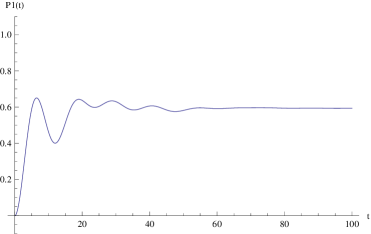
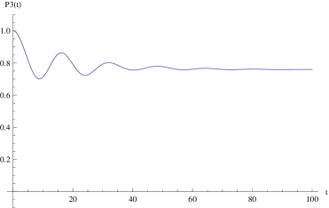
Figure 2: $P_{1}(t)$ (top left), $P_{2}(t)$ (top right) and $P_{3}(t)$ (bottom) for $\mu_{1,2}^{(0)}=0.2$, $\mu_{1,3}^{(0)}=0.1$, $\mu_{2,3}^{(0)}=0.15$, $\nu_{k,l}^{(0)}=\tilde{}\lambda_{j}=0$, $\omega_{1}=0.1$, $\omega_{2}=\omega_{3}=0.2$, $\Omega_{1}=\Omega_{3}=1$, $\Omega_{2}=2$, $\Omega=0.1$, $\lambda_{1}=0.1$, $\lambda_{2}=0.2$, $\lambda_{3}=0.05$, and $n_{1}=0$, $n_{2}=n_{3}=1$, $N_{1}=0$, $N_{2}=N_{3}=N=1$.

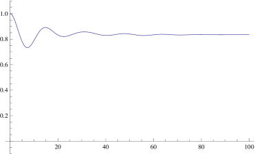
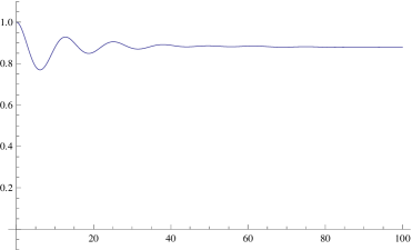
Figure 3: $P_{1}(t)$ (top left), $P_{2}(t)$ (top right) and $P_{3}(t)$ (bottom) for $\nu_{1,2}^{(0)}=0.1$, $\nu_{1,3}^{(0)}=0.08$, $\nu_{2,3}^{(0)}=0.1$, $\mu_{k,l}^{(0)}=\tilde{}\lambda_{j}=0$, $\omega_{1}=0.1$, $\omega_{2}=\omega_{3}=0.2$, $\Omega_{1}=\Omega_{3}=1$, $\Omega_{2}=2$, $\Omega=0.1$, $\lambda_{1}=0.1$, $\lambda_{2}=0.2$, $\lambda_{3}=0.05$, and $n_{1}=n_{2}=n_{3}=1$, $N_{1}=N_{2}=1$, $N_{3}=N=0$.

From both figures we see that, with these choices of parameters and initial conditions, the three DFs begin oscillating and then reach some asymptotic value, which is not just zero or one. In [1] we have discussed why this is so, and when a sharp result can be really deduced. The conclusion, here, is that it is quite unlikely that the traders reach some decision they are completely satisfied with. However, see for instance $P_{1}(t)$ and $P_{2}(t)$ in Figure 3, the asymptotic values of both these DFs are close to one. Hence, we see that the decision process produces a sort of unique decision. On the other hand, $\mathcal{P}_{3}$ is not really sure of what he has to do, since $P_{3}(t)$ for large $t$ approaches 0.4, which is not so close to zero.

A different story is described by Figure 4, where we are assuming that the traders only interact among themselves and not with any $\mathcal{R}_{j}$ or with $\mathcal{R}_{und}$. When this happens it is clear that none of the traders is able to reach a final decision on whether to buy or sell the asset. They just oscillate between different feelings, but a conclusion can only be reached when the traders also have some input from the larger sets of informed and noise traders.

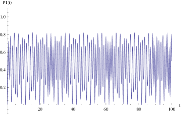
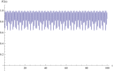
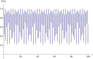
Figure 4: $P_{1}(t)$ (top left), $P_{2}(t)$ (top right) and $P_{3}(t)$ (bottom) for $\nu_{1,2}^{(0)}=0.1$, $\nu_{1,3}^{(0)}=0.08$, $\nu_{2,3}^{(0)}=0.1$, $\mu_{1,2}^{(0)}=2$, $\mu_{1,3}^{(0)}=1$, $\mu_{2,3}^{(0)}=3$, $\tilde{}\lambda_{j}=\lambda_{j}=0$, $\omega_{1}=0.1$, $\omega_{2}=\omega_{3}=0.2$, $\Omega_{1}=\Omega_{3}=\Omega=0.1$, $\Omega_{2}=0.2$ and $n_{1}=0$, $n_{2}=n_{3}=1$, $N_{1}=N_{2}=1$, $N_{3}=N=0$.

IV Conclusions

In this paper we have shown how to use operatorial techniques, and an Heisenberg-like dynamics, to describe two different, but somehow related, decision making processes. One such process is related to political alliances and the other process relates to buy and sell phenomena. A non-linear model which extends the model proposed in [1], has been introduced and an approximate procedure for the solution of the related equations of motion has also been proposed. We postpone to a second part of the paper the explicit analysis of these solutions, and a detailed analysis of the role of the parameters of the model. We claim that, for small values of the parameters governing the non-linearity, and for time intervals sufficiently small, these solutions do not differ significantly from those deduced in [1]. It is of course of interest to check what happens for longer intervals, and this will form part of a forthcoming project. Also, it can be interesting to extend the system described in Figure 1 adding more arrows. In particular, a natural extension of the model discussed in Section II can be constructed by admitting that, for instance, $\mathcal{P}_{1}$ also interacts with $\mathcal{R}_{2}$ and $\mathcal{R}_{3}$ (i.e. to try to convince them to change their intentions of vote).

Appendix: A few results on the number representation

To keep the paper self-contained, we discuss here a few important facts in quantum mechanics and in the so–called number representation.

Let $\mathcal{H}$ be a Hilbert space, and $B(\mathcal{H})$ the set of all the (bounded) operators on $\mathcal{H}$. Let $\mathcal{S}$ be our physical system, and ${\mathfrak{A}}$ the set of all the operators useful for a complete description of $\mathcal{S}$, which includes the observables of $\mathcal{S}$. For simplicity, it is convenient (but not really necessary) to assume that ${\mathfrak{A}}$ coincides with $B(\mathcal{H})$ itself. The description of the time evolution of $\mathcal{S}$ is related to a self–adjoint operator $H=H^{\dagger}$ which is called the hamiltonian of $\mathcal{S}$, and which in standard quantum mechanics represents the energy of $\mathcal{S}$. In this paper, we have adopted the so–called Heisenberg representation, in which the time evolution of an observable $X\in{\mathfrak{A}}$ is given by

$$X(t)=\exp(iHt)X\exp(-iHt),$$ (A.1)

or, equivalently, by the solution of the differential equation

$$\frac{dX(t)}{dt}=i\exp(iHt)[H,X]\exp(-iHt)=i[H,X(t)],$$ (A.2)

where $[A,B]:=AB-BA$ is the commutator between $A$ and $B$. The time evolution defined in this way is a one–parameter group of automorphisms of ${\mathfrak{A}}$.

An operator $Z\in{\mathfrak{A}}$ is a constant of motion if it commutes with $H$. Indeed, in this case, equation (A.2) implies that $\dot{Z}(t)=0$, so that $Z(t)=Z$ for all $t$.

In some previous applications, [2], a special role was played by the so–called canonical commutation relations. Here, these are replaced by the so–called canonical anti–commutation relations (CAR): we say that a set of operators $\{a_{\ell},\,a_{\ell}^{\dagger},\ell=1,2,\ldots,L\}$ satisfy the CAR if the conditions

$$\{a_{\ell},a_{n}^{\dagger}\}=\delta_{\ell n}1\!\!1,\hskip 22.76219pt\{a_{\ell},a_{n}\}=\{a_{\ell}^{\dagger},a_{n}^{\dagger}\}=0$$ (A.3)

hold true for all $\ell,n=1,2,\ldots,L$. Here, $1\!\!1$ is the identity operator and $\{x,y\}:=xy+yx$ is the anticommutator of $x$ and $y$. These operators, which are widely analyzed in any quantum mechanics textbook (see, for instance, [16, 17]) are those which are used to describe $L$ different modes of fermions. From these operators we can construct $\hat{n}_{\ell}=a_{\ell}^{\dagger}a_{\ell}$ and $\hat{N}=\sum_{\ell=1}^{L}\hat{n}_{\ell}$, which are both self–adjoint. In particular, $\hat{n}_{\ell}$ is the number operator for the $\ell$–th mode, while $\hat{N}$ is the number operator of $\mathcal{S}$. Compared with bosonic operators, the operators introduced here satisfy a very important feature: if we try to square them (or to rise to higher powers), we simply get zero: for instance, from (A.3), we have $a_{\ell}^{2}=0$. This is related to the fact that fermions satisfy the Fermi exclusion principle [17].

The Hilbert space of our system is constructed as follows: we introduce the vacuum of the theory, that is a vector $\varphi_{\mathbf{0}}$ which is annihilated by all the operators $a_{\ell}$: $a_{\ell}\varphi_{\mathbf{0}}=0$ for all $\ell=1,2,\ldots,L$. Such a non zero vector surely exists. Then we act on $\varphi_{\mathbf{0}}$ with the operators $a_{\ell}^{\dagger}$ (but not with higher powers, since these powers are simply zero!):

$$\varphi_{n_{1},n_{2},\ldots,n_{L}}:=(a_{1}^{\dagger})^{n_{1}}(a_{2}^{\dagger})^{n_{2}}\cdots(a_{L}^{\dagger})^{n_{L}}\varphi_{\mathbf{0}},$$ (A.4)

$n_{\ell}=0,1$ for all $\ell$. These vectors form an orthonormal set and are eigenstates of both $\hat{n}_{\ell}$ and $\hat{N}$: $\hat{n}_{\ell}\varphi_{n_{1},n_{2},\ldots,n_{L}}=n_{\ell}\varphi_{n_{1},n_{2},\ldots,n_{L}}$ and $\hat{N}\varphi_{n_{1},n_{2},\ldots,n_{L}}=N\varphi_{n_{1},n_{2},\ldots,n_{L}},$ where $N=\sum_{\ell=1}^{L}n_{\ell}$. Moreover, using the CAR, we deduce that

$$\hat{n}_{\ell}\left(a_{\ell}\varphi_{n_{1},n_{2},\ldots,n_{L}}\right)=(n_{\ell}-1)(a_{\ell}\varphi_{n_{1},n_{2},\ldots,n_{L}})$$

and

$$\hat{n}_{\ell}\left(a_{\ell}^{\dagger}\varphi_{n_{1},n_{2},\ldots,n_{L}}\right)=(n_{\ell}+1)(a_{l}^{\dagger}\varphi_{n_{1},n_{2},\ldots,n_{L}}),$$

for all $\ell$. Then $a_{\ell}$ and $a_{\ell}^{\dagger}$ are called the annihilation and the creation operators. Notice that, in some sense, $a_{\ell}^{\dagger}$ is also an annihilation operator since, acting on a state with $n_{\ell}=1$, we destroy that state.

The Hilbert space $\mathcal{H}$ is obtained by taking the linear span of all these vectors. Of course, $\mathcal{H}$ has a finite dimension. In particular, for just one mode of fermions, $dim(\mathcal{H})=2$. This also implies that, contrarily to what happens for bosons, all the fermionic operators are bounded.

The vector $\varphi_{n_{1},n_{2},\ldots,n_{L}}$ in (A.4) defines a vector (or number) state over the algebra ${\mathfrak{A}}$ as

$$\omega_{n_{1},n_{2},\ldots,n_{L}}(X)=\langle\varphi_{n_{1},n_{2},\ldots,n_{L}},X\varphi_{n_{1},n_{2},\ldots,n_{L}}\rangle,$$ (A.5)

where $\langle\,,\,\rangle$ is the scalar product in $\mathcal{H}$. As we have discussed in [2], these states are useful to project from quantum to classical dynamics and to fix the initial conditions of the considered system.

References

[1] F. Bagarello, An operator view on alliances in politics, SIAM Journal on Applied Mathematics (SIAP), 75, (2), 564–584
(2015)
[2] F. Bagarello, Quantum dynamics for classical
systems: with applications of the Number operator, Wiley Ed., New York,
(2012)
[3] O. A. Davis, M. J. Hinich, P. Ordeshook, An Expository
Development of a Mathematical Model of the Electoral Process, The American
Political Science Review, 64, No. 2, 426-448 (1970)
[4] P. Khrennikova, E. Haven, A. Khrennikov, An
application of the theory of open quantum systems to model the dynamics of
party governance in the US Political System, International Journal of
Theoretical Physics, 53, No. 4, 1346-1360 (2014)
[5] S. Galam, Majority Rule, Hierarchical Structures, and
Democratic Totalitarianism: A Statistical Approach, Journal of Mathematical
Psychology, 30, 426-434 (1986)
[6] S. Galam, The Drastic Outcomes from Voting Alliances
in Three-Party Democratic Voting (19902013), Journal of
Statistical Physics, 151, 46-68 (2013)
[7] M. Asano, M. Ohya, Y. Tanaka, I. Basieva, A. Khrennikov,
Quantum-like model of brain’s functioning: decision making from
decoherence, Journal of Theoretical Biology, 281, 56-64 (2011)
[8] F. Bagarello, E. Haven, The role of information in a
two-traders market, Physica A, 404, 224–233, (2014)
[9] F. Bagarello, E. Haven, Towards a formalization of a
two traders market with information exchange, Physica Scripta, 90,
015203 (2015)
[10] R. Mantegna, E. Stanley, An introduction to
econophysics, Cambridge University Press, (2000)
[11] J. Scheinkman, W. Xiong, Hetergenuous
beliefs, speculation and trading in financial markets, Paris-Princeton
Lectures Lectures on Mathematical Finance. LNM 1847, Springer Verlag (2004)
[12] S. Bikhchandani, J. Hirshleifer, J. Riley, The
analytics of uncertainty and information, Cambridge University Press (2013)
[13] E. Haven, A. Khrennikov, Quantum social science,
Cambridge University Press (2013)
[14] C. Ma, Advanced asset pricing theory, Imperial
College Press (2011)
[15] M. Brunnermeier, Asset pricing under asymmetric
information, Oxford University Press (2001)
[16] E. Merzbacher. Quantum Mechanics, Wiley, New York (1970)
[17] P. Roman, Advanced quantum mechanics, Addison–Wesley, New
York (1965)