Pion Generalized Parton Distributions within a fully covariant constituent quark model

Abstract

We extend the investigation of the Generalized Parton Distribution for a charged pion within a fully covariant constituent quark model, in two respects: (i) calculating the tensor distribution and (ii) adding the treatment of the evolution, needed for achieving a meaningful comparison with both the experimental parton distribution and the lattice evaluation of the so-called generalized form factors. Distinct features of our phenomenological covariant quark model are: (i) a 4D Ansatz for the pion Bethe-Salpeter amplitude, to be used in the Mandelstam formula for matrix elements of the relevant current operators, and (ii) only two parameters, namely a quark mass assumed to hold $m_{q}=~{}220$ MeV and a free parameter fixed through the value of the pion decay constant. The possibility of increasing the dynamical content of our covariant constituent quark model is briefly discussed in the context of the Nakanishi integral representation of the Bethe-Salpeter amplitude.

1 Introduction

The present theory of strong interaction, the Quantum Chromodynamics (QCD), should in principle allow one to achieve a complete 3D description of hadrons, in terms of the Bjorken variable $x_{B}$ and the transverse momenta of the constituents. As it is well-known, the needed non perturbative description still represents a challenge, that motivates a large amount of valuable efforts, both on the experimental side (gathering new accurate data, that in turn impose stringent constraints on theoretical investigations) and the theoretical one (performing more and more refined lattice calculations and elaborating more and more reliable phenomenological models).

Heuristically, while the short-distance behavior of the hadronic state has been well understood, given the possibility of applying a perturbative approach, entailed by the asymptotic freedom, the long-range part of the hadronic state, that is governed by the confinement, requests non perturbative tools, suitable for a highly non linear dynamics. Coping with the difficult task to gain information on the hadronic state, in the whole range of its extension, has been the main motivation for elaborating phenomenological models, that in general play a helpful role in shedding light onto the non perturbative regime.

Among the phenomenological approaches, covariant constituent quark models (CCQMs) represent an important step forward, since they exploit a quark-hadron vertex fulfilling the fundamental property of covariance with respect to the Poincaré group. Moreover, CCQM’s based on the Light-front (LF) framework, introduced by Dirac in 1949 Dirac , with variables defined by: $a^{\pm}=a^{0}\pm a^{3}$ and ${\bf a}_{\perp}\equiv\{a_{x},a_{y}\}$, appear to be quite suitable for describing relativistic, interacting systems, like hadrons. Indeed, the LF framework has several appealing features (see, e.g., Brodpr ), quite useful for exploring nowadays issues in hadronic phenomenology. Beyond the well-known fact that the dynamics onto the light-cone is naturally described in terms of LF variables, one should mention : (i) the straightforward separation of the global motion from the intrinsic one (related to the subgroup property of the LF boosts), (ii) the largest number of kinematical (i.e. not affected by the interaction) Poincaré generators, (iii) the large extent of triviality of the vacuum, within a LF field theory Brodpr (with the caveat of the zero-mode contributions). In particular, for the pion, one can construct the following meaningful Fock expansion onto the null-plane

$$|\pi\rangle=~{}|q\bar{q}\rangle~{}~{}+|q\bar{q}~{}q\bar{q}\rangle~{}+~{}|q\bar{q}~{}g\rangle.....$$

where $|q\bar{q}\rangle$ is the valence component. It has to be recalled that an appealing feature of our approach, based on a covariant description of the quark-pion vertex (see Frede09 ; Frede11 and references quoted therein), is the possibility of naturally taking into account contributions beyond the valence term.

The experimental efforts are very intense for singling out quantities that are sensitive to the dynamical features of the hadronic states. In particular, in the last decade, it has been recognized that a wealth of information on the 3D partonic structure of hadrons is contained in the Generalized Parton Distributions (GPDs) (see, e.g., Ref. Diehlpr for a general presentation), as well as in the Transverse-momentum Distributions (TMDs) (see, e.g., Ref. Baronpr for a detailed discussion). GPDs can be experimentally investigated through the Deeply Virtual Compton Scattering (DVCS), while TMDs can be studied through Semi-inclusive Deep Inelastic Scattering (SIDIS) processes, which notably involve polarization degrees of freedom.

Our aim, is to provide a phenomenological model, that has the following main ingredients: (i) a 4D Ansatz for the pion Bethe-Salpeter amplitude, and (ii) the generalization of the Mandelstam formula Mandel for matrix elements of the relevant current operators (notice that the pion Bethe-Salpeter amplitude is needed in this formula). Remarkably, we introduce only two parameters, namely a constituent quark mass and a free parameter fixed through the value of the pion decay constant. Through our model, we investigate the pion state by thoroughly comparing the results with both experimental and lattice data relevant for the 3D description of the pion. In this paper, we complete the evaluation of the leading-twist pion GPDs, calculating the so-called tensor GPD (see Ref. Frede09 for the vector GPD and Ref. Pace12 ; Pace13 for preliminary calculations of the tensor one). Moreover, in order to accomplish the previously mentioned comparisons, we consider the evolution of quantities that can be extracted from the GPDs, like the parton distribution function (PDF) and the generalized form factors (GFF). We anticipate that only the leading order (LO) evolution has been implemented by using the standard code of Ref. Kumano . In particular, the comparison has been performed between our LO results and the experimental pion PDF extracted in Ref. Conway (see Ref. Holt for the NLO extraction) and the available lattice calculations of GFFs as given in Refs. Bromth ; Lat07 ; Brom08 ; Brom08b .

The paper is organized as follows. In Sec. 2, the general formalism and the definitions are briefly recalled. In Sec. 3, our Covariant Constituent Quark Model is presented. In Sec. 4, the LO evolution of the quantities we want to compare is thoroughly discussed, with a particular care to the determination of the initial scale of our model. In Sec. 5, the comparison of our results with both the experimental PDF and the available lattice calculations is presented. Finally in Sec. 6, the Conclusion are drawn.

2 Generalities

In this Section, the physical quantities, GPDs and TMDs, that allow us to achieve a detailed 3D description of a pion are shortly introduced, since they represent the target of the investigation within our CCQM (for accurate and extensive reviews on GPDs, see, e.g. Diehlpr and on TMDs, see, e.g. Baronpr ). For the pion, given its null total angular momentum, one has two GPDs and two TMDs, at the leading twist.

2.1 Generalized Parton Distributions

As it is well known, GPDs are LF-boost invariant functions, and allow one to parametrize matrix elements (between hadronic states) involving quark and gluon fields. In particular, GPDs are off-diagonal (respect to the hadron four-momenta, i.e. $p_{f}\neq p_{i}$,) matrix elements of quark-quark (or gluon-gluon) correlator projected onto the Dirac basis (see, e.g., Ref. Meis08 for a thorough investigation of the pion case). The appealing feature of GPDs is given by the ability of summarizing in a natural way information contained in several observables investigated in different kinematical regimes, like electromagnetic (em), form factors (FFs) or PDFs.

The pion has two leading-twist quark GPDs: i) the vector, or no spin-flip, GPD, $H^{I}_{\pi}(x,\xi,t)$, and ii) the tensor, or spin-flip, GPD, $E^{I}_{\pi,T}(x,\xi,t)$ (where $I=IS,IV$ labels isoscalar and isovector GPDs, respectively). In order to avoid Wilson-line contributions, one can choose the light-cone gauge Diehlpr and get

$$2~{}\left(\begin{array}[]{c}H^{IS}_{\pi}(x,\xi,t)\\ {}\hfil\\ H^{IV}_{\pi}(x,\xi,t)\end{array}\right)=\int{dk^{-}d{\bf k}_{\perp}\over 2}$$ (4)

$$\times\int\frac{dz^{-}dz^{+}d{\bf z}_{\perp}}{2(2\pi)^{4}}e^{i[(xP^{+}z^{-}+k^{-}z^{+})/2-{\bf z}_{\perp}\cdot{\bf k}_{\perp}]}$$

$$\times~{}\langle p^{\prime}|\bar{\psi}_{q}(-\frac{1}{2}z)\gamma^{+}\left(\begin{array}[]{c}1\\ {}\hfil\\ \tau_{3}\end{array}\right)\psi_{q}(\frac{1}{2}z)|p\rangle=\int\frac{dz^{-}}{4\pi}$$ (8)

$$\times~{}e^{i(xP^{+}z^{-})/2}~{}\langle p^{\prime}|\bar{\psi}_{q}(-\frac{1}{2}z)\gamma^{+}\left(\begin{array}[]{c}1\\ {}\hfil\\ \tau_{3}\end{array}\right)\psi_{q}(\frac{1}{2}z)|p\rangle\big{|}_{\tilde{z}=0}$$ (12)

(13)

and

$$\frac{P^{+}\Delta^{j}-P^{j}\Delta^{+}}{P^{+}m_{\pi}}\left(\begin{array}[]{c}E^{IS}_{\pi T}(x,\xi,t)\\ {}\hfil\\ E^{IV}_{\pi T}(x,\xi,t)\end{array}\right)=\int\frac{dz^{-}}{4\pi}$$ (17)

$$\times~{}e^{i(xP^{+}z^{-})/2}~{}\langle p^{\prime}|\bar{\psi}_{q}(-\frac{1}{2}z)~{}i\sigma^{+j}~{}\left(\begin{array}[]{c}1\\ {}\hfil\\ \tau_{3}\end{array}\right)\psi_{q}(\frac{1}{2}z)|p\rangle\big{|}_{\tilde{z}=0}$$ (21)

(22)

where $\tilde{z}\equiv\{z^{+}=z^{0}+z^{3},{\bf z}_{\perp}\}$, $\psi_{q}(z)$ is the quark-field isodoublet and the standard GPD variables are given by

$$x={k^{+}\over P^{+}}~{}~{},\quad\xi=~{}-~{}{\Delta^{+}\over 2P^{+}}~{}~{},\quad t=\Delta^{2}~{}~{},$$

$$\Delta=p^{\prime}-p~{}~{},\quad P={p^{\prime}+p\over 2}$$ (23)

with the initial LF momentum of the active quark equal to $\{k^{+}-\Delta^{+}/2,{\bf k}_{\perp}-{\bf\Delta}_{\perp}/2\}$. The factor of two multiplying the vector GPD is chosen for normalization purpose, so that for a charged pion one has

$$F_{\pi}(t)=\int_{-1}^{1}dx~{}H^{IV}_{\pi}(x,\xi,t)=\int_{-1}^{1}dx~{}H^{u}_{\pi}(x,\xi,t)$$ (24)

where $H^{u}_{\pi}=H^{IS}_{\pi}+H^{IV}_{\pi}$, and $H^{IS}_{\pi}$ is odd in $x$ while $H^{IV}_{\pi}$ is even (see, e.g. Frede09 ). Finally, it is useful for what follows to recall the relation with the parton distributions, $q(x)$, viz

$$H^{u}_{\pi}(x,0,0)=\theta(x)u(x)-\theta(-x)\bar{u}(-x)~{}~{}.$$ (25)

At the present stage, only a few moments of the pion GPDs have been evaluated within lattice QCD, but they represent a valuable test ground for any phenomenological model that aspires to yield meaningful insights into the pion dynamics. In view of the numerical results discussed below, we briefly recall how the Mellin moments can be covariantly parametrized through the GFFs, that are the quantities adopted for comparing lattice calculations and phenomenological results.

The relation between the non-spin flip GPD and the em FF given in Eq. (24) for a charged pion can be in some sense generalized, if one considers Mellin moments of both vector and tensor GPDs. Then one obtains the corresponding GFFs. For instance, one can write the following Mellin moments of both vector and tensor GPDs for the $u$-quark (see Diehlpr ; Hagelpr for a review)

$$\int_{-1}^{1}dx\,x^{n}H^{u}_{\pi}(x,\xi,t)=\sum_{i=0}^{[(n+1)/2]}(2\xi)^{2i}A^{u}_{n+1,2i}(t)~{}~{},$$ (26)

$$\int_{-1}^{1}dx\,x^{n}E^{u}_{\pi,T}(x,\xi,t)=\sum_{i=0}^{[(n+1)/2]}(2\xi)^{2i}B^{u}_{n+1,2i}(t)$$ (27)

where the symbol $[...]$ indicates the integer part of the argument. In Eqs. (26) and (27), $A^{u}_{n+1,2i}(t)$ is a vector GFF for a $u$-quark and $B^{u}_{n+1,2i}(t)$ a tensor GFF, respectively. It is worth noting that one can introduce a different decomposition in terms of isoscalar and isovector components instead of a flavor decomposition. In particular, if $n+1$ is even (odd) one has an isoscalar (isovector) GFF. A striking feature is shown by the rhs of Eqs. (26) and (27), the so-called polinomiality, i..e. the dependence upon finite powers of the variable $\xi$. This polynomiality property follows from completely general properties like covariance, parity and time-reversal invariance; for this reason it can be a good test for any model.

By considering the first vector and tensor moments one gets the following important relations

$$\int_{-1}^{1}dx\,H^{u}_{\pi}(x,\xi,t)=A^{u}_{1,0}(t)=F_{\pi}(t)$$ (28)

and

$$\int_{-1}^{1}dx\,E^{u}_{\pi,T}(x,\xi,t)=B^{u}_{1,0}(t)$$ (29)

where $B^{u}_{1,0}(0)\neq 0$ is the tensor charge for $n=0$, also called tensor anomalous magnetic moment (see Ref. Hagelpr ). Notably, Eq. (26) leads to the following relation involving the Mellin moments of the PDF and $A^{u}_{n+1,0}(0)$, viz

$$<x^{n}>_{u}=\int_{-1}^{1}dx\,x^{n}H^{u}_{\pi}(x,0,0)=A^{u}_{n+1,0}(0)$$ (30)

A physical interpretation of GFFs (see, e.g., Bur ; Bur05 ; Bur08 ) can be achieved by properly generalizing the standard interpretation of the non relativistic em FFs to a relativistic framework. Non relativistically, the em FFs are the 3D Fourier transforms of intrinsic (Galilean-invariant) em distributions in the coordinate space (e.g., for the pion, one has the charge distribution, while, for the nucleon, one has both charge and magnetic distributions). In the relativistic case, one should consider Fourier transforms of GPDs, that depend upon variables invariant under LF boosts. Indeed, only the transverse part of $\Delta^{\mu}$ can be trivially conjugated to variables in the coordinate space, while for $x$ and $\xi$ (proportional to $\Delta^{+}$) this is not possible. Therefore, keeping the description invariant for proper boosts (i.e. LF boosts), one can introduce 2D Fourier transforms with respect to ${\bf\Delta}_{\perp}$. Such a Fourier transform allows one to investigate the spatial distributions of the quarks in the so-called impact-parameter space (IPS). In particular, from Eq. (26) and (27), it straightforwardly follows that, for $\xi=0$, only $A^{u}_{n+1,0}(\Delta^{2})$ and $B^{u}_{n+1,0}(\Delta^{2})$ survive. Due to the LF-invariance of $\xi$, one has an infinite set of frames (Drell-Yan frames) where $\xi=0$. In these frames, where $\Delta^{+}=0$ and $\Delta^{2}=-\Delta^{2}_{\perp}$, one can introduce the above mentioned 2D Fourier transforms in a boost-invariant way (recall that, for a given reaction, the final state or both final and initial states have to be boosted). One can write

$$\tilde{A}^{q}_{n}(b_{\perp})=\int{d{\bf\Delta}_{\perp}\over(2\pi)^{2}}~{}e^{i{\bf\Delta}_{\perp}\cdot{\bf b}_{\perp}}A^{q}_{n,0}(\Delta^{2})~{},$$

$$\tilde{B}^{q}_{n}(b_{\perp})=\int{d{\bf\Delta}_{\perp}\over(2\pi)^{2}}~{}e^{i{\bf\Delta}_{\perp}\cdot{\bf b}_{\perp}}B^{q}_{n,0}(\Delta^{2})$$ (31)

where $b_{\perp}=|{\bf b}_{\perp}|$, is the impact parameter. In general, the Fourier transform of GFFs, for $\xi=0$, yield quark densities in the IPS Bur ; Bur05 ; Bur08 . In particular, $\tilde{A}_{n}(b_{\perp})$ represents the probability density of finding an unpolarized quark in the pion at a certain distance $b_{\perp}$ from the transverse center of momentum. In addition, if one considers the polarization degrees of freedom, then one introduces the probability density of finding a quark with a given transverse polarization, ${\bf s}_{\perp}$ in a certain Drell-Yan frame. In the IPS, such a probability distribution is

$$\rho^{q}_{n}({\bf b}_{\perp},{\bf s}_{\perp})=\frac{1}{2}\left[\tilde{A}^{q}_{n}(b_{\perp})+\frac{s^{i}\epsilon^{ij}b^{j}}{b_{\perp}}~{}\Gamma^{q}_{n}(b_{\perp})\right]$$ (32)

where

$$\Gamma^{q}_{n}(b_{\perp})=-\frac{1}{2m_{\pi}}\frac{\partial~{}\tilde{B}^{q}_{n}(b_{\perp})}{\partial~{}b_{\perp}}$$ (33)

It is worth noting that the quark longitudinal (or helicity) distribution density is given only by the first term in Eq. (32), since the pion is a pseudoscalar meson and the term $\gamma_{5}\hbox to0.0pt{/\hss}s_{L}$ in the quark density operator has a vanishing expectation value, due to the parity invariance Brom08b ; Diehl05 .

Equation (32) is quite rich of information and clearly indicates the pivotal role of GPDs for accessing the quark distribution in the IPS. Moreover, as a closing remark, one could exploit the spin-flip GPD $E^{q}_{\pi T}$ to extract more elusive information on the quasi-particle nature of the constituent quarks, like their possible anomalous magnetic moments, once the vector current that governs the quark-photon coupling is suitably improved (see subsect. 5.4 and Ref. Brom07 for a discussion within the lattice framework).

2.2 Transverse momentum distributions

TMDs are diagonal (in the pion four-momentum) matrix elements of the quark-quark (or gluon-gluon) correlator with the proper Wilson-line contributions (see, e.g., Ref. Meis08 ) and suitable Dirac structures. Moreover, TMDs depend upon $x$ and the quark transverse momentum, ${\bf k}_{\perp}$, that is not the conjugate of ${\bf b}_{\perp}$. It should be pointed out that in general the Wilson-line effects must be carefully analyzed, due to the explicit dependence upon ${\bf k}_{\perp}$ (recall that for GPDs such dependence is integrated out). At the leading-twist, one has two TMDs, for the pion: the T-even $f^{q}_{1}(x,|{\bf k}_{\perp}|^{2})$, that yields the probability distribution to find an unpolarized quark with LF momentum $\{x,{\bf k}_{\perp}\}$ in the pion, and the T-odd $h^{q\perp}_{1}(x,|{\bf k}_{\perp}|^{2},\eta)$, related to a transversely-polarized quark and called Boer-Mulders distribution Boer .

The two TMDs allow one to parametrize the distribution of a quark with given LF momentum and transverse polarization, i.e. (see, e.g., Ref. Brom08 ; Meis08 )

$$\rho^{q}(x,{\bf k}_{\perp},{\bf s}_{\perp},\eta)=$$

$$=\frac{1}{2}\Bigl{[}f^{q}_{1}(x,|{\bf k}_{\perp}|^{2})+{s^{i}\epsilon^{ij}k_{\perp}^{j}\over m_{\pi}}~{}h^{q\perp}_{1}(x,|{\bf k}_{\perp}|^{2},\eta)\Bigr{]}$$ (34)

where the dependence upon the variable $\eta$ in $h^{\perp}_{1}$ is generated by the Wilson-line effects, whose role is essential for investigating a non vanishing $h^{\perp}_{1}$ (see e.g. Boer ).

At the lowest order, the unpolarized TMD $f^{q}_{1}$, is given by the proper combination of the isoscalar and isovector components, that are defined by

$$2\left(\begin{array}[]{c}f^{IS}_{1}(x,|{\bf k}_{\perp}|^{2})\\ {}\hfil\\ f^{IV}_{1}(x,|{\bf k}_{\perp}|^{2})\end{array}\right)=\int{dz^{-}d{\bf z}_{\perp}\over 2(2\pi)^{3}}e^{i[xP^{+}z^{-}/2-{\bf k}_{\perp}\cdot{\bf z}_{\perp}]}$$ (38)

$$\times~{}\langle p|\bar{\psi}_{q}(-\frac{1}{2}z)\gamma^{+}\left(\begin{array}[]{c}1\\ {}\hfil\\ \tau_{3}\end{array}\right)\psi_{q}(\frac{1}{2}z)|p\rangle\big{|}_{z^{+}=0}~{}~{}~{},$$ (42)

After integrating over ${\bf k}_{\perp}$, one gets the standard unpolarized parton distribution $q(x)$, viz

$$q(x)=\int d{\bf k}_{\perp}~{}f^{q}_{1}(x,|{\bf k}_{\perp}|^{2})=~{}H^{q}_{1}(x,0,0)~{}~{}~{}.$$ (43)

The T-odd TMD, $h^{\perp}_{1}(x,|{\bf k}_{\perp}|^{2},\eta)$ needs a more careful analysis, since it vanishes at the lowest order in perturbation theory. As a matter of fact, it becomes proportional to the matrix elements

$$\langle p|\bar{\psi}_{q}(-\frac{1}{2}z)~{}i~{}\sigma^{+j}~{}\left(\begin{array}[]{c}1\\ {}\hfil\\ \tau_{3}\end{array}\right)\psi_{q}(\frac{1}{2}z)|p\rangle\big{|}_{z^{+}=0}~{}~{}~{},$$ (47)

that are equal to zero, due to the time-reversal invariance. In order to get a non vanishing Boer-Mulders distribution, one has to evaluate at least a first-order correction, involving Wilson lines (see, e.g., Refs. Lu04 and Meis08 ). Moreover, by adopting the light-cone gauge and the advanced boundary condition for the gauge field, the effect of the Wilson lines (final state interaction effects) can be shifted into complex phases affecting the initial state (see, e.g., Ref. Beli03 ).

3 The Covariant Constituent Quark Model

The main ingredients of our covariant constituent quark model are two: i) the extension to the GPDs and TMDs of the Mandelstam formalism Mandel , originally introduced for calculating matrix elements of the em current operator when a relativistic interacting system is investigated, and ii) a model of the 4D quark-hadron vertex, or equivalently the Bethe-Salpeter amplitude, necessary for applying the Mandelstam approach. In particular, we have assumed a pion Bethe-Salpeter amplitude (BSA) with the following form

$$\Psi(t,p)=-{m\over f_{\pi}}~{}S\left(t+p/2\right)~{}\Gamma(t,p)~{}S\left(t-p/2\right)$$

(48)

where $p=p_{q}+p_{\bar{q}}$ is the total momentum, $t=(p_{q}-p_{\bar{q}})/2$ the relative momentum of the $q\bar{q}$ pair (by using the four-momenta $k$, $\Delta$ and $P$ previously introduced, one has $t+p/2=k-\Delta/2$, and $t-p/2=k-P$). In Eq. (48), $S(p_{q})=1/(\hbox to0.0pt{/\hss}p_{q}-m_{q}+\imath\epsilon)$ is the fermion propagator and $\Gamma(t,p)$ the quark-pion vertex. In the present work, only the dominant Dirac structure has been assumed, viz

$$\Gamma(t,p)=\gamma_{5}~{}\Lambda_{\pi}(t,p)$$ (49)

with $\Lambda(t,p)$ a suitable momentum-dependent scalar function that contains the dynamical information (see the following subsections for more details). Indeed, Dirac structures contributing to $\Gamma(t,p)$ beyond $\gamma^{5}$ should be taken into account, but they have a minor impact on the pion BSA, as thoroughly discussed in Ref. maris .

For the sake of completeness, let us recall that the quark-pion vertex fulfills the homogeneous BS equation that reads as follows

$$\Gamma(t,p)=$$

$$=\int{d^{4}t^{\prime}\over(2\pi)^{4}}~{}{\cal K}(t,t^{\prime})~{}S\left(t^{\prime}+p/2\right)~{}\Gamma(t^{\prime},p)~{}S\left(t^{\prime}-p/2\right)$$

where ${\cal K}(t,t^{\prime})$ is the kernel given by the infinite sum of irreducible diagrams (see, e.g., IZ ).

Finally, it is important to emphasize that our investigation, based on a covariant description of the quark-pion vertex, naturally goes beyond a purely valence description of the pion Frede09 ; Frede11 .

3.1 The Mandelstam Formula for the electromagnetic current

The Mandelstam formula allows one to express the matrix elements of the em current of a composite bound system, within a field theoretical approach Mandel . It has been applied for evaluating the FFs of both pion Melo02 ; Melo04 ; Melo06 and nucleon Melo09 , obtaining a nice description of both space- and timelike FFs. Furthermore, it has been exploited for calculating the vector GPD of the pion Frede09 ; Frede11 and for a preliminary evaluation of the tensor GPD Pace12 ; Pace13 .

For instance, in the case of the em spacelike FF of the pion, the Mandelstam formula, where the quark-pion vertex given in Eq. (49) is adopted, reads (see, e.g., Ref. Melo02 ; Melo04 ; Melo06 )

$$j^{\mu}~{}=~{}-\imath e~{}{\cal R}$$

$$\times~{}\int\frac{d^{4}k}{(2\pi)^{4}}\Lambda_{\pi}(k+\Delta/2,p^{\prime})\Lambda_{\pi}(k-\Delta/2,p)$$

$$\times~{}Tr[S(k-P)\gamma^{5}S(k+\Delta/2)V^{\mu}(k,q)S(k-\Delta/2)\gamma^{5}]$$

(51)

where ${\cal R}=2N_{c}m^{2}_{q}/f^{2}_{\pi}$, $f_{\pi}$ is the pion decay constant $N_{c}=3$ the number of colors, $m_{q}$ the CQ mass and $V^{\mu}(k,q)$ the quark-photon vertex, that we have simplified to $\gamma^{\mu}$ in the spacelike region. In presence of a CQ, one could add to the bare vector current a term proportional to an anomalous magnetic moment, namely a term like

$$i{\kappa_{q}\over 2m_{q}}\sigma^{\mu\nu}\Delta_{\nu}~{}~{}~{},$$

as in Ref. Brom07 (where it has been adopted an improved vector current within a lattice framework). It should be pointed out that the above mentioned anomalous magnetic moment is not used in the present work.

Within CCQM, the expression of the decay constant in term of $\Lambda_{\pi}$ reads (cf Ref. Melo02 )

$$f_{\pi}=-i\frac{m_{q}}{f_{\pi}}{N_{c}\over m^{2}_{\pi}}\int\frac{d^{4}k}{(2\pi)^{4}}~{}\Lambda_{\pi}(k-\Delta/2,p)$$

$$\times~{}Tr\Bigl{[}\hbox to0.0pt{/\hss}p\gamma_{5}S(k-\Delta/2)\gamma_{5}S(k-P)\Bigr{]}=$$

$$=i\frac{m_{q}^{2}~{}N_{c}}{(2\pi)^{2}f_{\pi}}\int{d\kappa^{+}\over\kappa^{+}~{}(\kappa^{+}-m_{\pi})}~{}\int d^{2}\kappa_{\perp}\Phi(\kappa^{+},\kappa_{\perp})$$ (52)

where $\kappa=k-\Delta/2=k-P+p$ (recall $p^{2}=m^{2}_{\pi}$), $\kappa_{\perp}=|{\bf\kappa}_{\perp}|$ and

$$\Phi(\kappa^{+},\kappa_{\perp})=\kappa^{+}~{}(\kappa^{+}-m_{\pi})\int{d\kappa^{-}\over 2\pi}$$

$$\times{\Lambda_{\pi}(\kappa,p)\over\Bigl{[}\kappa^{2}-m^{2}_{q}+i\epsilon\Bigr{]}~{}\Bigl{[}(\kappa-p)^{2}-m^{2}_{q}+i\epsilon\Bigr{]}}~{}$$ (53)

is the valence wave function. It should be recalled that $\Phi$, properly integrated on $\kappa_{\perp}$, yields the pion distribution amplitude (DA) (see Eq. (95) and, e.g., Ref. Diehlpr for a general discussion on the DAs and their evolution). The generalization of Eq. (51) to the case of GPDs, can be found in Ref. Frede09 ; Frede11 for the vector GPD, and in Pace12 ; Pace13 for the tensor one, but for the sake of completeness, let us give the expression of both vector and tensor GPDs for the $u$ quark, viz

$$2~{}H^{u}(x,\xi,t)=-\imath{\cal R}~{}\int\frac{d^{4}k}{(2\pi)^{4}}~{}\delta[P^{+}x-k^{+}]$$

$$\times~{}\Lambda(k-P,p^{\prime})\;\;\Lambda(k-P,p)$$

$$\times~{}Tr\left[S\left({k}-{P}\right)\gamma^{5}S\left({k}+\Delta/2\right)\gamma^{+}S\left({k}-\Delta/2\right)\gamma^{5}\right]$$

(54)

and

$${P^{+}\Delta^{j}-P^{j}\Delta^{+}\over~{}P^{+}m_{\pi}}E^{u}_{\pi T}(x,\xi,t)=$$

$$=i{\cal R}\int\frac{d^{4}k}{(2\pi)^{4}}\delta[P^{+}x-k^{+}]~{}\Lambda(k-P,p^{\prime})~{}\Lambda(k-P,p)$$

$$\times Tr[S({k}-{P})\gamma^{5}S({k}+\Delta/2)\gamma^{+}\gamma^{j}S({k}-\Delta/2)\gamma^{5}]~{}$$ (55)

where $j=1,2$. The $\delta$ function allows one to have the correct support for the active quark, i.e. when $|\xi|\leq x\leq 1$. This kinematical region corresponds to the so-called Dokshitzer-Gribov-Lipatov-Altarelli-Parisi (DGLAP) region dglap1 ; dglap2 ; dglap3 , or valence region. Moreover, CCQM is able to address also kinematical region beyond the valence one, i.e. $-\xi\leq x\leq\xi$, given the covariance property. This region is called the Efremov-Radyushkin-Brodsky-Lepage (ERBL) region erbl1 ; erbl2 , or non valence region. If one adopts a Breit frame with $\Delta^{+}=-\Delta^{-}\geq 0$, then the ERBL region can be investigated. As a matter of fact, in such a frame one can access the whole range of the variable $\xi$, i.e. $-1\leq\xi\leq 1$, and analyze both valence and non valence regions within the same approach. This allows one to shed light on the interesting topic of the smooth transition from the DGLAP (valence) regime to the ERBL (non valence) one.

The expression of the unpolarized TMD $f^{q}_{1}(x,|{\bf k}_{\perp}|^{2})$ Frede09 can be easily obtained from the integrand of the vector GPD, Eq. (54), by recalling the relation in Eq. (43).

3.2 The four-momentum dependence of the Bethe-Salpeter amplitude

As above mentioned, in our CCQM we focus on the main contribution to the pion BSA, i.e. the term containing the Dirac matrix $\gamma_{5}$. This implies that we have to consider only one scalar function for describing the dependence upon the four-momenta present in the problem. Unfortunately, solutions of the homogeneous BSE for hadrons are still lacking in Minkowski space given the extraordinary complexity of QCD, nonetheless very relevant investigations have been carried out in Euclidean space, within the lattice framework Bromth ; Lat07 ; Brom08 ; Brom08b or combining BSE and Dyson-Schwinger equation (DSE) (see, e.g., Holt10 and references quoted therein) or by exploiting a 3D reduction of the BSE itself (see, e.g., Gross14 ). On the other hand, since we would carry on a comparison with a wide set of data, from both experiments and lattice, we resort to adopt a phenomenological Ansatz, that depends remarkably upon only two parameters. This allows us to explore the potentiality of the Mandelstam approach in capturing the main features of the physical quantities under consideration, while having a reasonable predictive power, given the small set of free parameters.

The following analytic covariant Ansatz for the momentum dependence of the BSA has been adopted

$$\Lambda(t,p)=$$

$$=C~{}{1\over\left[(t+p/2)^{2}-m^{2}_{R}+\imath\epsilon\right]}~{}{1\over\left[(t-p/2)^{2}-m^{2}_{R}+\imath\epsilon\right]}$$

(56)

where the parameter $m_{R}$ is adjusted to fit $f_{\pi}$, while the constants $C$ is fixed through the charge normalization, $F_{\pi}(t=0)=1$, that amounts to the standard normalization of the BSA, but in impulse approximation.

It is worth noting that the expression in Eq. (56) can be cast (see below) in a form suggested by the integral representation of the 4D $n$-leg transition amplitudes (we are actually interested to the $3$-leg amplitude, i.e. the vertex $\pi\to q\bar{q}$) elaborated by Nakanishi in the 60’s Naka , within a perturbation-theory framework. To quickly illustrate the appealing features of this integral representation, one should consider the $n$-leg transition amplitude for a many-scalar interacting system, and the infinite set of Feynman diagrams contributing to determine the amplitude itself. In this case, it turns out that the amplitude is given by the folding of a weight function (called the Nakanishi weight function) and a denominator (with some exponent) that contains all the independent scalar products obtained from the $n$ external four-momenta. It has to be pointed out that the analytic behavior of the amplitude is fully determined by such a denominator, and this clearly makes the Nakanishi integral representation a valuable tool for investigating 4D transition amplitudes. For $n=3$, one can apply the integral representation to the vertex function for a system composed by two constituents, and explicitly discuss the analytic structure, i.e. the core of the physical content. Another pivotal motivation that increases the interest on the Nakanishi framework is given by the following computational finding: even if the Nakanishi integral representation has been formally established by considering the whole infinite set of the Feynman diagrams contributing to an amplitude, i.e. a perturbative regime, it has been numerically shown that also in a non perturbative framework, like the homogeneous BSE (relevant for describing bound systems), the Nakanishi representation plays an essential role for obtaining actual solutions for the vertex function or, equivalently, for the BSA. Applying the Nakanishi representation as an Ansatz for the solution of the BSE one can determine the unknown Nakanishi weight function and achieve a genuine numerical solution of the BSE in Minkowski space. This approach has been applied to the ladder BSE for two-scalar and two-fermion systems (see, e.g.,Refs. CK06 ; CK10 ; Frede12 ; Frede14 ; Frede15 for the Nakanishi approach in Minkowski space and, for the sake of comparison, Ref. Dork1 ; Dork2 for two-fermion systems within the Euclidean hyperspherical approach), opening a viable path for phenomenological studies within a non perturbative regime.

Within the Nakanishi approach, the vertex function (or three-leg amplitude) can be written as follows

$$\Lambda(t,p)=~{}\int_{0}^{\infty}d\gamma\int^{1}_{-1}dz~{}{g(\gamma,z;\kappa^{2})\over\Bigl{[}\gamma+\kappa^{2}-t^{2}-z~{}p\cdot t-i\epsilon\Bigr{]}^{2}}$$

(57)

where $\kappa^{2}=m^{2}_{q}-p^{2}/4$ and $g(\gamma,z;\kappa^{2})$ is called Nakanishi weight function. If we take $g(\gamma,z;\kappa^{2})=\delta(\gamma-m^{2}_{R}+m^{2}_{q})$, one obtains Eq. (56). It should be pointed out that while waiting for numerical solutions of the two-fermion system with more refined phenomenological kernels (for the ladder approximation see Ref. CK10 ), one could perform an intermediate step, still in the realm of Ansatzes, substituting Eq. (56) with Eq. (57), but adopting a different choice of the Nakanishi weight function, e.g. by substituting the simple delta-like form with more realistic functions (see e.g. Frede14 for the Nakanishi weight functions of a two-scalar system obtained by actually solving the homogeneous BSE in the ladder approximation). In order to set the reference line for the next steps in the elaboration of our CCQM (presented elsewhere), we will adopt the very manageable form given in Eq. (56), in the following comparisons with the experimental and lattice results (see below, Sec. 5).

4 Evolution of Mellin Moments and GFF’s

In order to compare our results for PDF and GFFs with experimental data and lattice calculations, it is fundamental to suitably evolve the CCQM outcomes, from the unknown scale $\mu_{CCQ}$ to the needed ones, namely $\mu_{exp}$ and $\mu_{LAT}$.

Our strategy for determining an acceptable $\mu_{CCQ}$ is to study the evolution of the non singlet PDF Mellin within a LO framework, considering flavor numbers up to $N_{f}=4$. It should be pointed out that the choice to adopt the LO framework, seems to be well motivated by the phenomenological nature of the CCQM, and by the present uncertainties still affecting both experimental and lattice GFFs.

Let us shortly summarize our procedure for assigning a scale $\mu$ to our calculations. The main ingredient to be considered are the Mellin moments of the non singlet distribution $f_{NS}(x,\mu)$, viz

$$M_{NS}(n,\mu)=\int_{0}^{1}dx~{}x^{n}~{}f_{NS}(x,\mu)$$ (58)

where $f_{NS}$ is related to the unpolarized GPD, as follows

$$f_{NS}(x,\mu_{CCQ})=2H^{I=1}(x,0,0)$$ (59)

Mellin moments evolve from a scale $\mu_{0}$ to the scale $\mu$ through very simple expressions (see, e.g., greiner ), that for the non singlet, singlet and gluon moments read

$$\frac{dM_{NS}(n,\mu)}{dln\mu^{2}}=\frac{\alpha_{s}^{LO}(\mu,N_{f})}{2\pi}\frac{\gamma^{(0)}_{qq}(n)}{2\beta_{0}}~{}M_{NS}(n,\mu)$$ (60)

$$\frac{d\overrightarrow{M}(n,\mu)}{dln\mu^{2}}=\frac{\alpha_{s}^{LO}(\mu,N_{f})}{2\pi}\frac{\Gamma^{(0)}(n)}{2\beta_{0}}~{}\overrightarrow{M}(n,\mu)$$ (61)

where

$$\overrightarrow{M}(n,\mu)=\left(\begin{array}[]{c}M_{S}(n,\mu)\\ M_{G}(n,\mu)\end{array}\right)$$ (64)

In Eqs. (60) and (61), the LO anomalous dimensions are indicated by $\gamma^{(0)}_{ab}$ while the $2\times 2$ matrix $\Gamma^{(0)}(n)$ is given by

$$\Gamma^{(0)}(n)=\left(\begin{array}[]{ccc}\gamma_{qq}^{(0)}(n)&{}\hfil&\gamma_{qG}^{(0)}(n)\\ &\\ \gamma_{Gq}^{(0)}(n)&{}\hfil&\gamma_{GG}^{(0)}(n)\end{array}\right).$$ (68)

Let us recall that each anomalous dimension $\gamma^{(0)}_{ab}(n)$ is obtained from the corresponding LO splitting function. In particular, for the unpolarized case, one has (see, e.g., greiner )

$$\gamma_{qq}^{(0)}(n)=-\frac{8}{3}\left[3+\frac{2}{(n+1)(n+2)}-4\sum_{k=1}^{n+1}\frac{1}{k}\right]$$ (69)

$$\gamma_{qG}^{(0)}(n)=-2\left[{n^{2}+3n+4\over(n+1)(n+2)(n+3)}\right]$$ (70)

$$\gamma_{Gq}^{(0)}(n)=-\frac{16}{3}\left[{n^{2}+3n+4\over n(n+1)(n+2)}\right]$$ (71)

$$\gamma_{GG}^{(0)}(n,N_{f})=-6\Bigl{[}{\beta_{0}(N_{f})\over 3}+8~{}{n^{2}+3n+3\over n(n+1)(n+2)(n+3)}$$

$$-4\sum_{k=1}^{n+1}\frac{1}{k}\Bigr{]}.$$ (72)

where

$$\beta_{0}(N_{f})=11-\frac{2}{3}N_{f}$$ (73)

By taking into account the eigenvalues of $\Gamma^{(0)}(n)$, given by (see anodimrad for details)

$$\gamma_{\pm}(n)=\frac{1}{2}\left[\gamma_{qq}^{(0)}(n)+\gamma_{GG}^{(0)}(n)\right.$$

$$\left.\pm\sqrt{(\gamma_{qq}^{(0)}(n)-\gamma_{GG}^{(0)}(n))^{2}+4\gamma_{qG}^{(0)}(n)\gamma_{Gq}^{(0)}(n)}\right]~{}~{},$$ (74)

one can write the $2\times 2$ matrix in terms of projectors and eigenstates as follows

$$\Gamma^{(0)}(n)=\gamma_{+}(n)\mathcal{P}_{+}(n)+\gamma_{-}(n)\mathcal{P}_{-}(n)$$ (75)

with

$$\mathcal{P}_{\pm}(n)=\frac{\pm 1}{\gamma_{+}(n)-\gamma_{-}(n)}[\Gamma^{(0)}(n)-\gamma_{\mp}(n)~{}{\rm I}]$$ (76)

They fulfills the usual projector properties, i.e.

$$\mathcal{P}_{+}+\mathcal{P}_{-}=1$$

$$\mathcal{P}_{\pm}^{2}=\mathcal{P}_{\pm}$$

$$\mathcal{P}_{+}\mathcal{P}_{-}=\mathcal{P}_{-}\mathcal{P}_{+}=0$$ (77)

Solutions of Eqs. (60) and (61) are given by

$$M_{NS}(n,\mu)=\left[\frac{\alpha_{s}^{LO}(\mu,N_{f})}{\alpha_{s}^{LO}(\mu_{0},N_{f})}\right]^{[\gamma^{(0)}_{NS}(n)/2\beta_{0}(N_{f})]}$$

$$\times~{}M_{NS}(n,\mu_{0})$$ (78)

$$\overrightarrow{M}(n,\mu)=\left[\frac{\alpha_{s}^{LO}(\mu,N_{f})}{\alpha_{s}^{LO}(\mu_{0},N_{f})}\right]^{[\Gamma^{(0)}(n)/2\beta_{0}(N_{f})]}$$

$$\times~{}\overrightarrow{M}(n,\mu_{0})$$ (79)

Notably, Eq. (79) can be put in a more simple form by using the eigenvalues, $\gamma_{\pm}$, and the corresponding projectors $\mathcal{P}_{\pm}$, viz. anodimrad

$$\overrightarrow{M}(n,\mu)=\Bigl{\{}\Bigl{[}\frac{\alpha_{s}^{LO}(\mu,N_{f})}{\alpha_{s}^{LO}(\mu_{0},N_{f})}\Bigr{]}^{[\gamma_{+}(n)/2\beta_{0}]}\mathcal{P}_{+}$$

$$+\Bigl{[}\frac{\alpha_{s}^{LO}(\mu,N_{f})}{\alpha_{s}^{LO}(\mu_{0},N_{f})}\Bigr{]}^{[\gamma_{-}(n)/2\beta_{0}]}\mathcal{P}_{-}\Bigr{\}}~{}\overrightarrow{M}(n,\mu_{0}).$$ (80)

Indeed, we are interested to actually evolve only the moment $n=1$ of $f_{NS}$, since for this moment we can find several lattice calculations (but using different approximations; cf Sec. 5). Our procedure requests to backward-evolve the lattice $M^{LAT}_{NS}(1,\mu_{LAT})$, down to a scale $\mu_{0}$ where $M^{LAT}_{NS}(1,\mu_{0})=M^{CCQM}_{NS}(1)$ (notice the absence of the unknown scale dependence in the CCQM first moment). This value of the scale is taken as $\mu_{CCQ}$. From Eq. (78), one recognizes the necessity to first determine $\alpha^{LO}_{s}(\mu_{LAT},N_{f})$. This can be accomplished starting from a reasonable value of $\alpha_{s}(\mu_{i},3)$, like $\alpha_{s}(\mu_{i}=1~{}GeV,3)=0.68183$ given in Ref. martin (see also Sect. 5 for the quantitative elaboration). To perform this step we have used the well-known expression

$$\alpha_{s}^{LO}(\mu,N_{f})=\frac{\alpha_{s}^{LO}(\mu_{i},N_{f})}{1+{\alpha_{s}^{LO}(\mu_{i},N_{f})\over 4\pi}\beta_{0}(N_{f})~{}\ln\Bigl{(}\mu^{2}/\mu_{i}^{2}\Bigr{)}}$$ (81)

It should be pointed out that, as explicitly shown in Eqs. (73) and (81), $\alpha_{s}(\mu,N_{f})$ depends upon the number of flavors $N_{f}$, at a given scale. Indeed, one has to be particularly careful about the energy scales involved, when one moves from a relatively low $\mu_{i}=1~{}{\rm GeV}$ to $\mu_{LAT}=2~{}{\rm GeV}$, large enough to produce a new quark flavor, so that $N_{f}$ increases from $3$ to $4$. In practice, a two-step procedure has been adopted for moving from $\alpha_{s}(\mu_{i},N_{f}=3)$ to $\alpha_{s}(\mu_{LAT},N_{f}=4)$, by properly changing $\beta_{0}(N_{f})$, at the threshold $\mu=m_{c}$, i.e the mass of the charm.

In what follows, it is also useful to define, at a given energy scale and number of flavors,

$$\ln(\Lambda^{N_{f}}_{QCD})=\ln(\mu)-{2\pi\over\beta_{0}(N_{f})~{}\alpha_{s}^{LO}(\mu,N_{f})}$$ (82)

4.1 QCD Evolution of GFFs

Similarly to the more familiar case of PDFs, where the QCD interaction among partons lead to ultraviolet divergences which are factored out and absorbed into a dependence upon the energy scale, also in the case of GPDs one has to deal with the issue of finding and solving evolution equations. As a matter of fact, GPDs do not depend on three variables but on four, namely $H(x,\xi,t,\mu)$ and $E(x,\xi,t,\mu)$. However, the evolution kernel does not depend on $t$, so that the relevant variables for the evolution are $x$, $\xi$, and $\mu$. One should keep in mind that the evolution of GPDs is produced by the combination of two regimes: (i) the one pertaining to the valence region ($|x|>|\xi|$) and (ii) the one pertaining to the non valence region ($|x|<|\xi|$). One could roughly say that the evolution of GPDs interpolates Diehlpr between the two regions and therefore the evolution kernel has to take into account the suitable physical content. In particular, in the valence region a kernel acts with a structure like the one present in the DGLAP equations, while in the non valence region a modified ERBL kernel is involved (see Refs. ji97 and TGPDevol for details on the evolution of vector and tensor GPDs, respectively).

In our actual comparison, we do not consider the full GPDs, but rather their Mellin moments, since they can be in principle addressed by the lattice calculations. As a matter of fact, GFFs covariantly parametrize the Mellin moments of GPD (see Eqs. (26) and (27)), and evolve through a suitable generalization of the Eqs. (78) and (79) (see Refs. anodimrad ; Broni08b ; Aevol ; Kivel ; Kirch ; Broni10 ; Broni11 ). Let us recall, however, that GFFs are the coefficients of polynomials in $\xi$ that yield the Mellin moments of GPDs and not the Mellin moments themselves: for this reason in general the equations describing GFFs evolution are more complicated than Eqs. (78) and (79). Indeed one can find some notable exceptions where the equations have a simple multiplicative structure.

For the vector GFFs $A^{I}_{ni}(t,\mu^{2})$, one should recall that the evolution of the isoscalar (singlet) GPD, and consequently the evolution of the corresponding Mellin moments, is coupled with the evolution of the gluonic component. This leads one to separate the evolution of GFFs with even and odd $n$, since for symmetry reasons the even GFFs come from the isoscalar GPDs, while the odd ones come from the isovector GPDs. By repeating the main steps given in Ref. Aevol (see also Kivel ; Kirch where general discussions are presented) for obtaining the evolution equation of both non singlet and singlet vector GFFs, we can express the results in Ref. Aevol also as follows

$$A_{2k+1,2\ell}(t,\mu)={\Gamma(2k+1)\over 2}~{}\sum_{j=k-\ell}^{k}~{}2^{2(j-k)}$$

$$\times~{}\sum_{m=j}^{k}~{}(4m+3)L_{2m+1}~{}{(-1)^{m-j}~{}\Gamma(j+m+3/2)\over\Gamma(2j+1)}$$

$$\times~{}{A_{2j+1,2(j-k+\ell)}(t,\mu_{0})\over\Gamma(m-j+1)\Gamma(k-m+1)\Gamma(k+m+5/2)}$$ (83)

with $0\leq\ell\leq k$ and

$$L_{2m+1}=\left(\frac{\alpha_{s}(\mu,N_{f})}{\alpha_{s}(\mu_{0},N_{f})}\right)^{[\gamma^{(0)}_{qq}(2m)/2\beta_{0}(N_{f})]}~{}~{}.$$ (84)

For the singlet vector GFFs we get

$$A_{2k+2,2\ell}(t,\mu)=\Gamma(2k+2)~{}\sum_{j=k-\ell}^{k}~{}2^{2(j-k)-1}$$

$$\times~{}\sum_{m=j}^{k}(4m+5)L_{2m+2}~{}{(-1)^{m-j}~{}\Gamma(j+m+5/2)\over\Gamma(2j+2)}$$

$$\times~{}{A_{2(j+1),2(j-k+\ell)}(t,\mu_{0})\over\Gamma(m-j+1)\Gamma(k-m+1)\Gamma(k+m+7/2)}$$ (85)

with $0\leq\ell\leq k+1$, $A_{00}=0$ and

$$L_{2m+2}=\left(\frac{\alpha_{s}(\mu,N_{f})}{\alpha_{s}(\mu_{0},N_{f})}\right)^{[\Gamma^{(0)}_{V}(2m+1)/2\beta_{0}(N_{f})]}$$ (86)

where $\Gamma^{(0)}_{V}$ is the same $2\times 2$ matrix defined in (68) that depends upon $N_{f}$ through $\gamma^{(0)}_{GG}$. In Eqs. (4.1) and (4.1), $\Gamma(k)$ is the usual Euler function. Notice that the dependence upon $t$ in the GFF is not involved in the evolution. Some example of explicit evolution equations are

$$A_{n0}(t,\mu)=L_{n}~{}A_{n0}(t,\mu_{0})$$

$$A_{22}(t,\mu)=L_{2}~{}A_{22}(t,\mu_{0})$$ (87)

where $A_{22}(t,\mu)$ is a 2D vector, with quark and gluon components, and $L_{2}$ a $2\times 2$ matrix. For $A_{n0}(t,\mu)$ the evolution equations become exactly equal to Eqs. (78) and (79) for the odd and even $n$’s respectively. Moreover, since $\gamma^{(0)}_{qq}(n=0)=0$ then $L_{1}=1$. This is expected since $A_{10}(t=0)$ is the charge ($A_{10}(t)$ is the em form factor), namely a measurable quantity and therefore it cannot evolve.

For the tensor GFF $B_{ni}^{I}(t,\mu)$, analogous arguments can be carried out, but with a great simplification. In fact, at LO the gluon-quark and quark-gluon transition amplitudes that lead to the corresponding splitting functions are vanishing for the helicity conservation (recall that $E_{T}(x,\xi,t)$ is related to an expectation value with a transversely polarized quark and describes helicity flip transitions), therefore the anomalous dimension matrix $\Gamma^{(0)}_{T}(n)$ is diagonal. Consequently, at LO it is not necessary to separate the case of even and odd $n$, since there is no mixing between quark and gluon evolutions, and one can eventually write the evolution equation in a form analogous to Eq. (4.1). In particular, the quark component of the transverse GFFs, $B^{q}_{n0}(t,\mu)$, evolves multiplicatively (see, e.g., anodimrad ; Broni10 ; Broni11 ; Nam11 ), viz

$$B^{q}_{n0}(t,\mu)=L_{n}^{qT}~{}B^{q}_{n0}(t,\mu_{0}).$$ (88)

where

$$L^{qT}_{n}=\left(\frac{\alpha_{s}(\mu,N_{f})}{\alpha_{s}(\mu_{0},N_{f})}\right)^{[\gamma_{qqT}^{(0)}(n-1)/2\beta_{0}(N_{f})]}$$ (89)

with a transverse anomalous dimension (notice a factor of 2 difference with anodimrad , due to the different normalization) given by

$$\gamma^{(0)}_{qqT}(\ell)=~{}-{8\over 3}~{}\Bigl{[}3-4\sum_{k=1}^{\ell+1}\frac{1}{k}\Bigr{]}~{}~{}.$$ (90)

For the sake of completeness, the gluon transverse LO anomalous dimension reads

$$\gamma^{(0)}_{ggT}(\ell)=~{}-6~{}\Bigl{[}{\beta_{0}(N_{f})\over 3}-4\sum_{k=1}^{\ell+1}\frac{1}{k}\Bigr{]}~{}~{}.$$ (91)

5 Numerical Results

The reliability of the quark-pion vertex (56), introduced for obtaining the Bethe-Salpeter amplitude (48), has been first checked by comparing our results for a charged pion with the most accurate experimental data not affected by the evolution, i.e. the spacelike em form factor. Theoretically, the em form factor, $F_{\pi}(t)$, is given by the GFF $A_{10}(t)$. In Fig. (1) the results obtained by different models for the em FF are shown as a function of $(-t)$, together with the experimental data. To avoid the use of a log plot, that prevents a detailed analysis, the FF has been divided by the monopole function

$$F_{mon}(t)=\frac{1}{1+|t|/m_{\rho}^{2}}$$ (92)

where $m_{\rho}=0.770$ GeV. Interestingly, in order to test the dependence upon the CQ mass, the results of our CCQM evaluated for quark masses $m_{q}=0.200$, $0.210$, $0.220$ GeV, have been also shown, together with (i) the results from a LF CQM where $m_{q}=0.265$ GeV and a dressed quark-photon vertex were adopted Melo04 ; Melo06 ; (ii) a fit to the lattice data obtained in Brom07 . It has to be pointed out that the fit to the lattice data was presented in Brom07 itself, and it has the following monopole expression

$$F^{lat}_{\pi}(t)=\frac{1}{1-t/M^{2}(m_{\pi}^{phys})}$$ (93)

with $M(m_{\pi}^{phys})=0.727$ GeV. The lattice results were actually obtained for a pion mass $m_{\pi}=0.600$ GeV, and then extrapolated to the physical pion mass $m_{\pi}^{phys}=0.140$ GeV, up to $t=-4~{}\textrm{GeV}^{2}$ (see Brom07 ). In Fig. (1), for the sake of presentation, the monopole fit (93) has been arbitrarily extended up to $t=-10\,\textrm{GeV}^{2}$. Once the CQ mass is assigned, our CCQM model depends upon only one free parameter, the regulator mass $m_{R}$ in Eq. (56). The value of $m_{R}$ is fixed by calculating the pion decay constant $f_{\pi}$ (cf Eq. (52)), while the constant $C$ is determined through $F_{\pi}(0)$, as already mentioned in subsec. 3.2. The PDG experimental value $f^{exp}_{\pi}=~{}0.0922$ GeV PDG14 has been adopted. In particular, for $m_{q}=0.200,~{}210,~{}220$ GeV, we got $m_{R}=~{}1.453$,$~{}1.320$,$~{}1.192$ GeV, respectively.

The following comments are in order: (i) a nice agreement between the CCQM results and the experimental FF at low momentum transfer leads to reproduce the experimental value of the charge radius, $<r^{2}_{exp}>=0.67\pm 0.02$ fm; (ii) beyond $-t=~{}0.5~{}{\rm GeV}^{\rm 2}$, CCQM results begin to reveal an interesting sensitivity upon the CQ mass, since if one changes the CQ mass by a 5% then the corresponding CCQM FF changes by 10-15%, at high momentum transfer; (iii) the CCQM FFs seem to have a similar curvature of the data at high momentum transfer, but in order to draw reliable conclusions, useful for extracting information (and then improving the CCQM), it is necessary to have more accurate data, for $-t\geq 1~{}{\rm GeV}^{2}$.

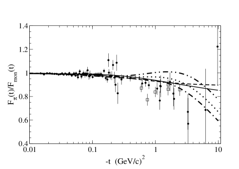
Figure 1: Charged pion form factor vs $-t$. Solid line: LF Constituent Quark Model with $m_{q}=0.265$ GeV Melo04 ; Melo06 . Dashed line: monopole fit to lattice data extrapolated to $m_{\pi}=0.140$ GeV as obtained in Brom07 , arbitrarily extended in this figure from $-4$ to $-10\,\textrm{GeV}^{2}$. Dot-dashed line: CCQM, cf Eq. (56), corresponding to a CQ mass $m_{q}=~{}0.220$ GeV and $m_{R}=~{}1.192$ GeV in the vertex (56) (recall that $m_{R}$ is obtained by fitting $f^{exp}_{\pi}=0.0922$ GeV PDG14 ). Dotted line: as the dot-dashed one, but with $m_{q}=0.210$ GeV and $m_{R}=1.320$ GeV. Double-dot-dashed line: as the dot-dashed one, but with $m_{q}=0.200$ GeV and $m_{R}=1.453$ GeV. Experimental data: as quoted in Frede09 .

Another interesting data set to be compared with is given by the photon-pion transition form factor, $F^{*}_{\pi}(-t)$, measured in the process $\gamma\gamma^{*}\to\pi^{0}$ BABAR ; BELLE . Within CCQM, only the LO asymptotic value of such transition FF can be evaluated without adding new ingredients (see, e.g., Ref. deTB11 for a wide discussion and references quoted therein). As a matter of fact, one gets for high $(-t)$, at LO in pQCD,

$$(-t)~{}F^{*}_{\pi}(-t)\to{2f_{\pi}\over 3}~{}\int_{0}^{1}d\xi~{}{\phi_{\pi}(\xi,|t|)\over\xi}$$ (94)

where $\phi_{\pi}(\xi,|t|)$ is the pion DA evaluated at the scale $|t|$. The CCQM result (with an undetermined scale for the moment, see the next subsection) is given by

$$\phi_{\pi}(\xi,\mu^{2}_{CCQM})=i{m^{2}_{q}N_{c}\over f^{2}_{\pi}m_{\pi}(2\pi)^{2}}$$

$$\times~{}{1\over\xi(1-\xi)}~{}\int_{0}^{\infty}d^{2}\kappa_{\perp}~{}\Phi(\xi m_{\pi},\kappa_{\perp})$$ (95)

where $\Phi(\xi m_{\pi},\kappa_{\perp})$ is defined in Eq. (53). The normalization of $\phi_{\pi}$ follows from Eq. (52). It should be anticipated that CCQM results, both non evolved and evolved, as shown in the next Fig. 3, resemble the asymptotic pion DA obtained within the pQCD framework, i.e. $\phi^{asy}_{\pi}(\xi)=6\xi(1-\xi)$, that in turn yields $(-t)~{}F^{*}_{\pi}(-t)\to~{}2f_{\pi}$, see Refs. LB80 ; BL81 .

In what follows, the values $m_{q}=0.220$ geV and $m_{R}=1.192$ GeV will be adopted.

5.1 Looking for the CCQM energy scale

As it is well-known, the em FF is not affected by the issue of the evolution, while the other quantities we are interested in, namely the PDF and the GFFs (as well as the DA, see Eq. (95)), have to be properly evolved.

A necessary step for going forward is to assign a resolution scale to CCQM. In order to perform this step, we have taken lattice estimates of the first Mellin moment of $f_{NS}(x,\mu)$, whose evolution is determined only by the quark contribution, as normalization of our CCQM (roughly speaking). The starting point is the calculation of both the unpolarized GPD, $f_{NS}(x)=2H^{I=1}(x,0,0)$, and the corresponding Mellin moments, within our CCQM. In particular, these quantities are shown in Table 1 up to $n=3$. To emphasize that there is no direct way to gather information about the energy scale $\mu_{0}$, a question mark is put in the Table.

Table 1: Mellin moments of $f_{NS}(x)$ up to $n=3$, evaluated within the CCQM with the quark pion vertex given in Eq. (56), $m_{q}=0.220$ GeV, and $m_{R}=1.192$ GeV. The energy scale, $\mu_{0}$ has to be determined (see text).

$\mu_{0}$	$<x>$	$<x^{2}>$	$<x^{3}>$
?	0.471	0.276	0.183

In the literature there are various lattice results for the first moment at the energy scale of $\mu=2$ GeV, and we have exploited the ones shown in Tab. 2. It is worth noticing that the lattice results are not too far from a phenomenological estimate, $<x>_{phe}(\mu=2~{}{\rm GeV})$, that one can deduce by applying a LO backward-evolution to the value given in Ref. Holt , $<x>_{phe}(\mu=5.2~{}{\rm GeV})=0.217(11)$, obtained after a NLO re-analysis of the Drell-Yan data of Ref. Conway . In particular, the phenomenological value at $\mu=2$ GeV is

$$<x>_{phe}(\mu=2~{}{\rm GeV})=0.260(13)$$

Table 2: Recent lattice results for the first Mellin moment of the non singlet $f_{NS}(x)$, at the energy scale $\mu_{LAT}=2$ GeV. The first and the second lines are the results obtained from unquenched lattice QCD calculations Lat07 ; south , while the third result has been obtained in quenched lattice QCD chilf .

Ref.	$\mu_{LAT}[GeV]$	$<x>_{LAT}$
Lat. 07 Lat07	2.0	0.271(10)
South south	2.0	0.249(12)
$\chi$LF chilf	2.0	0.243(21)

For the sake of completeness, it is interesting to quote two other lattice calculations: (i) the quenched one of Ref. twist that amounts to a value $<x>_{LAT}(\mu=2~{}{\rm GeV})=0.246(15)$, i.e. falling between the results of Refs. south ; chilf and (ii) a very recent lattice estimate, remarkably at the physical pion mass, giving $<x>_{LAT}(\mu=2~{}{\rm GeV})=0.214(19)$ twist2 .

After establishing the set of lattice data, we need the value of $\alpha_{s}^{LO}$ at $\mu=2$ GeV where $N_{f}=4$. This value has been obtained starting from $\alpha_{s}^{LO}(\mu=1~{}{\rm GeV})=0.68183$ obtained in Ref. martin . Notice that at the scale $\mu=1~{}{\rm GeV}$ only three flavors are active. Then, by using $m_{c}=1.4$ GeV martin and Eq. (81), with the proper $\beta_{0}(N_{f})$, one determines $\alpha^{LO}_{s}(\mu=2~{}{\rm GeV},4)=0.413$ (see also Refs. PDG14 ; Marciano ; MRST , where the crossing of the flavor threshold has been discussed). Finally, paying attention to the flavor threshold, the lattice evaluations of the first moment $M^{LAT}_{NS}(1,\mu_{LAT})$ have to be backward-evolved up to a scale $\mu_{0}$, where they match our CCQM value, i.e. we look for $\mu_{0}$ such that $M^{LAT}_{NS}(1,\mu_{0})=0.471=M^{CCQM}_{NS}(1,?)$.

Table 3: Energy scale of CCQM, $\mu_{0}$, as determined from (i) the first Mellin moments calculated within a lattice framework in Refs. Lat07 ; south ; chilf and (ii) the CCQM result, $<x>=0.471$, calculated with $m_{q}=0.220$ GeV and $m_{R}=1.192$ GeV. For all the three calculations shown in the Table, one gets $\Lambda^{N_{f}=3}_{QCD}(\mu_{0})=0.359$ GeV from Eqs. (82) and (98).

Ref.	$<x>_{LAT}$	$\mu_{0}$ [GeV]	$\alpha^{LO}_{s}(\mu_{0},3)$
Lat. 07 Lat07	0.271	0.549	1.64
South south	0.249	0.506	2.04
$\chi$LF chilf	0.243	0.496	2.17

Table 4: Comparison for the second and third Mellin moments of the non singlet $f_{NS}(x)$, at the energy scale $\mu_{LAT}=2$ GeV, between the unquenched lattice results of Ref. Lat07 and the evolved CCQM, where the theoretical uncertainty is generated by the three values for the CCQM initial scale shown in Tab. 3

	$<x^{2}>$	$<x^{3}>$
Lat. 07 Lat07	0.128(18)	0.074(27)
CCQM	0.105(11)	0.055(7)

In detail, we calculate first (cf. Eq. (78)) the lattice result at the charm mass scale, viz

$$M_{NS}(1,m_{c})=\left[\frac{\alpha^{LO}_{s}(m_{c},4)}{\alpha^{LO}_{s}(\mu_{LAT},4)}\right]^{\gamma^{(0)}_{qq}(1)/(2\beta_{0}(4))}$$

$$\times~{}M_{NS}(1,\mu_{LAT})$$ (96)

where $\gamma^{(0)}_{qq}(1)=64/9$, $\beta_{0}(4)=25/3$, $\alpha_{s}^{LO}(m_{c},4)=0.513$ (corresponding to $\Lambda_{QCD}(N_{f}=4)=0.322$ GeV) and $M_{NS}(1,\mu_{LAT})$ are the values shown in Tab. 2. Once $M_{NS}(1,m_{c})$ is obtained, $\alpha_{s}^{LO}(\mu_{0})$ can be evaluated through (cf. Eq. (78))

$$\alpha^{LO}_{s}(\mu_{0},3)=\alpha_{s}^{LO}(m_{c},3)$$

$$\times~{}\left[\frac{M_{NS}(1,\mu_{0})}{M_{NS}(1,m_{c})}\right]^{-\gamma^{(0)}_{qq}(1)/(2\beta_{0}(3))}~{},$$ (97)

where $M_{NS}(1,\mu_{0})$ corresponds to our CCQM calculation and $\beta_{0}(3)=9$. After determining $\alpha^{LO}_{s}(\mu_{0},3)$, $\mu_{0}$ is easily found through

$$\ln\left({\mu_{0}\over\mu=1~{}{\rm GeV}}\right)={2\pi\over\beta_{0}(3)}$$

$$\times~{}\Bigl{[}{1\over\alpha^{LO}_{s}(\mu_{0},3)}-{1\over\alpha^{LO}_{s}(\mu=1~{}{\rm GeV},3)}\Bigr{]}$$

(98)

The results for $\mu_{CCQ}$ obtained from the above procedure, applied to the three lattice data, are shown in Tab. 3 for $m_{q}=0.220$ GeV and $m_{R}=1.192$ GeV. In particular, the values in the third column of Tab. 3 are used in the next sections as starting values for the evolution of both the non singlet PDF and the GFFs. The difference between the three values of $\mu_{0}$ in the Tab. 3 is assumed as a theoretical uncertainty of our results. To complete this subsection, in Tab. 4, the comparison with the lattice calculation of Ref. Lat07 for the second and the third Mellin moments is presented.

5.2 The evolution of the non singlet PDF and the comparison with the experimental data

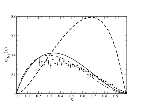
Figure 2: Evolution of the non singlet parton distribution. Dashed line: non evolved PDF obtained from CCQM $H^{I=1}(x,0,0)$ with a CQ mass $m_{q}=0.220$ GeV and $m_{R}=1.192$ GeV in the vertex (56). Solid line: PDF LO-evolved at $\mu=4$ GeV from $\mu_{0}=0.549$ GeV. Dot-dashed line: PDF LO-evolved at $\mu=4$ GeV from $\mu_{0}=0.496$ GeV. For details on the values of $\mu_{0}$ see text and Tab. 3. Full dots: experimental data at the energy scale $\mu=4$ GeV, as given in Ref. Conway

The non singlet PDF, as already explained, is the simplest to be evolved since one does not need information on the gluon distribution. The evolution has been performed using the FORTRAN code described in Kumano that adopts a brute force method to solve the LO DGLAP equation for the distribution $xf_{NS}(x)$, and it requests as input the values of (i) $\mu$, the final scale, and (ii) the initial $\Lambda^{N_{f}}_{QCD}$ and $\mu_{0}$, as given in Table 3. It should be pointed out an important detail in our calculations. For all the values of $\mu_{0}$, the evolution has been performed in two steps: first $xf^{CCQM}_{NS}(x)$ has been evolved from $\mu_{0}$ up to $m_{c}=1.4$ GeV and then from $m_{c}$ up to $\mu=4$ GeV, the energy scale of the experimental data Conway . This is necessary for taking into account the variation of $N_{f}$, $\Lambda_{QCD}$(recall that $\Lambda^{N_{f}=4}_{QCD}(\mu=2~{}GeV)$ is $0.322$ GeV) and consequently $\alpha_{s}^{LO}(\mu)$.

In Fig. 2, the dashed line is the non evolved CCQM calculation with $m_{q}=0.220$ GeV and $m_{R}=1.192$ GeV, while the solid and the dot-dashed lines correspond to our evolved CCQM starting from the initial scales $\mu_{0}=0.549$ GeV and $\mu_{0}=0.496$ GeV, respectively. The differences between the evolved calculations can be interpreted as the theoretical uncertainty of our calculations. However it is very interesting that our LO-evolved calculations nicely agree with the experimental data of Ref. Conway for $x>0.5$ (see also the same agreement achieved within the chiral quark model of Ref. Broni08b ). On the other hand, it has to be pointed out that refined calculations, like (i) the ones of Refs. Hecht ; Chang14 based on the Euclidean Dyson-Schwinger equation for the self-energy and (ii) the NLO calculation of Ref. Aicher based on a soft-gluon resummation, underestimate the PDF tail of the experimental data from Ref. Conway , while agree with the analysis of the same experimental data carried out in Ref. Holt , within a NLO framework. The reanalysis of the experimental data leads to a tail for large $x$ that has a rather different derivative with respect to the original data from Ref. Conway .

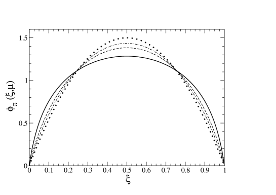
Figure 3: Evolution of the pion distribution amplitude. Solid line: non evolved DA obtained from our CCQM with $m_{q}=0.220$ GeV and $m_{R}=1.192$ GeV in the vertex (56) (see Eqs. (53) and (95)). Dashed line: DA LO-evolved at $\mu=1$ GeV. Dot-dashed line: PDF LO-evolved at $\mu=6$ GeV. Dotted line: pQCD asymptotic DA, given by $\phi_{\pi}(\xi)=6\xi(1-\xi)$.

For the sake of completeness, in Fig. 3, the CCQM pion DA is presented together with the results at the energy scale $\mu=1$ GeV and $\mu=6$ GeV. It is worth noticing that our CCQM evolves toward the pQCD asymptotic pion DA $\phi_{\pi}(\xi)=6~{}\xi~{}(1-\xi)$ (see, e.g., LB80 ; BL81 ) as the energy scale increases. Analogous results are obtained within the chiral quark model of Ref. Broni08 .

5.3 The tensor GPD

We have extended to the tensor GPD our CCQM model already applied to the vector GPD in Refs. Frede09 ; Frede11 , and in Fig. 4, our final results are shown for some values of the variable $\xi$ and $t$, but for $0\leq x\leq 1$ (preliminary results were presented in Refs. Pace12 ; Pace13 ). The GPD for negative values of $x$ can be obtained by exploiting the fact that $E^{IS}_{\pi T}(x,\xi,t)$ is antisymmetric if $x\to~{}-x$, while $E^{IV}_{\pi T}(x,\xi,t)$ is symmetric (see, e.g. Ref. Diehlpr for details). It has to be pointed out that for $\xi\to 0$ the valence component is dominant (DGLAP regime) while for $\xi\to 1$ the non valence term is acting (ERBL regime). In view of that, it is expected a peak around $x\sim 1$ for $\xi\to 1$, as discussed in Refs. Frede09 ; Frede11 for the vector GPD.

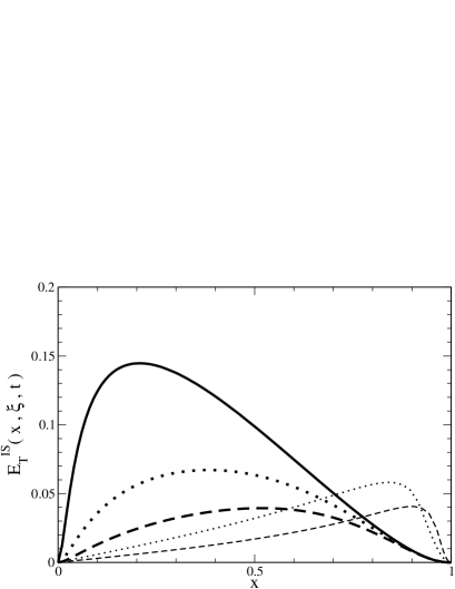
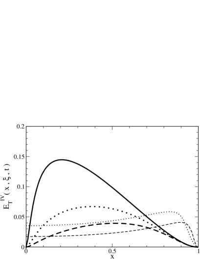
Figure 4: Isoscalar and isovector tensor GPDs for a charged pion, within CCQM, for positive $x$. The behavior for negative values of $x$ can be deduced from the antisymmetry of $E^{IS}_{\pi T}(x,\xi,t)$ and the symmetry of $E^{IV}_{\pi T}(x,\xi,t)$, respectively. Thick solid line: $\xi=0~{}$ and $t=0$. Thick dotted line: $\xi=0~{}$ and $t=-0.4\,GeV^{2}$. Thick dashed line: $\xi=0~{}$ and $t=-1\,GeV^{2}$. Thin dotted line: $\xi=0.96$ and $t=-0.4\,GeV^{2}$. Thin dashed line: $\xi=0.96$ and $t=-1\,GeV^{2}$.

It is worth mentioning that both isoscalar and isovector tensor GPD calculated within the chiral quark model of Ref. Broni11 qualitatively show the same pattern (see also Ref. Pace12 and reference therein quoted for a comparison with results obtained within the LF Hamiltonian Dynamics framework).

5.4 The evolution of the GFFs and the comparison with lattice data

The first vector GFF $A^{q}_{10}$, i.e. the em FF, is experimentally known, while the other GFFs can be investigated only from the theoretical side. In particular, $A^{q}_{20}(t,\mu)$, $A^{q}_{22}(t,\mu)$, $B^{q}_{10}(t,\mu)$ and $B^{q}_{20}(t,\mu)$ have been calculated within the lattice framework at the scale $\mu=2$ GeV Bromth ; Brom08 ; Brom08b . In this subsection, the comparison between our CCQM predictions and the above mentioned lattice evaluations is presented. It is important to notice that other model calculations of both vector and tensor GFFs are available in the literature (see, e.g., Broni10 ; Broni11 ; Nam11 ; Broni08 ; Aribron ; Diehl10 ).

To proceed, we have calculated both vector and tensor GPDs, and then we have extracted the relevant GFFs, by exploiting the polynomiality shown in Eqs. (26) and (27) (see also Frede09 ). The main issue to be addressed in order to perform the mentioned comparison with the lattice data is the evolution of our calculations up to $\mu_{LAT}=2$ GeV. In the simpler case, represented by the tensor GFFs, the LO evolution of the quark contribution is uncoupled from the gluon one. In particular, the two-step procedure $\mu_{CCQ}\to m_{c}\to\mu_{LAT}$ has been adopted for evolving the two transverse GFFs, $B^{q}_{10}(t,\mu_{0})$ and $B^{q}_{20}(t,\mu_{0})$, through Eq. (88). The needed transverse anomalous dimensions are given by (cf. Eq. (90))

$$\gamma_{qqT}^{(0)}(0)=\frac{8}{3}~{}~{},\quad\quad\quad\gamma_{qqT}^{(0)}(1)=8~{}~{}.$$ (99)

Then, for $\mu_{CCQ}\leq\mu<m_{c}$ one has $N_{f}=3$ and gets

$$B^{q}_{10}(t,m_{c})=B^{q}_{10}(t,\mu_{CCQ})\left[\frac{\alpha^{LO}_{s}(m_{c},3)}{\alpha_{s}^{LO}(\mu_{CCQ},3)}\right]^{4/27}$$ (100)

$$B^{q}_{20}(t,m_{c})=B^{q}_{20}(t,\mu_{CCQ})\left[\frac{\alpha^{LO}_{s}(m_{c},3)}{\alpha_{s}^{LO}(\mu_{CCQ},3)}\right]^{4/9}$$ (101)

For $m_{c}\leq\mu\leq\mu_{LAT}$, the flavor number is $N_{f}=4$ and one has

$$B^{q}_{10}(t,\mu_{LAT})=B^{q}_{10}(t,m_{c})\left[\frac{\alpha^{LO}_{s}(\mu_{LAT},4)}{\alpha_{s}^{LO}(m_{c},4)}\right]^{4/25}$$ (102)

$$B^{q}_{20}(t\mu_{LAT})=B^{q}_{20}t,(m_{c})\left[\frac{\alpha^{LO}_{s}(\mu_{LAT},4)}{\alpha_{s}^{LO}(m_{c},4)}\right]^{12/25}.$$ (103)

In the case of $A_{20}(t,\mu)$ and $A_{22}(t,\mu)$ the evolution equation is more complicated, since both GFFs evolve through the following expression

$$\overrightarrow{A}_{2i}(t,\mu)=L_{2}\overrightarrow{A}_{2i}(t,\mu_{0})$$ (104)

where, for both scales, one has

$$\overrightarrow{A}_{2i}=\left(\begin{array}[]{c}A^{q}_{2i}\\ \\ A^{G}_{2i}\end{array}\right)$$ (108)

From the definition (86), the exponent in $L_{2}$ is a $2\times 2$ matrix, (see also Eqs. (68), (69), (70), (71) and (72)) that for $N_{f}=3$ reads

$$\Gamma^{(0)}_{V}(1)=\left(\begin{array}[]{ccc}\gamma_{qq}^{(0)}(1)&{}\hfil&\gamma_{qG}^{(0)}(1)\\ &{}\hfil&\\ \gamma_{Gq}^{(0)}(1)&{}\hfil&\gamma_{GG}^{(0)}(1)\end{array}\right)=\left(\begin{array}[]{ccc}\frac{64}{9}&{}\hfil&-\frac{2}{3}\\ &{}\hfil&\\ -\frac{64}{9}&{}\hfil&4\end{array}\right)$$ (115)

with eigenvalues (see Eq. (4))

$$\gamma_{\pm}=\frac{50\pm 2\sqrt{145}}{9}~{}~{}~{}.$$ (116)

At the valence scale, the gluon contribution is vanishing, and therefore one has $<x>_{q}=1/2$. Indeed, the CCQM result amounts to $<x>(\mu_{CCQ})=0.47$, namely the momentum sum rule is not completely saturated by the valence component at the CCQM scale $\mu_{CCQ}$. This difference originates from the fact that we have a covariant description of the pion vertex, and therefore we have not only a contribution from the valence LF wave function (i.e. the amplitude of the Fock component with the lowest number of constituents), but also from components of the Fock expansion of the pion state beyond the constituent one, like $|q\bar{q};q\bar{q}\rangle$. Without the gluon term at the initial scale (the assumed valence one), $A_{2i}^{q}(t,m_{c})$ is given by (cf. Eqs. (75) and (76))

$$A_{2i}^{q}(t,m_{c})=\frac{1}{2\sqrt{145}}A_{2i}^{q}(t,\mu_{CCQ})~{}{\cal R}_{3}^{25/81}$$

$$\times~{}\Bigl{[}(7+\sqrt{145})~{}{\cal R}_{3}^{\sqrt{145}/81}-(7-\sqrt{145})~{}{\cal R}_{3}^{-\sqrt{145}/81}\Bigr{]}~{}~{},$$

where

$${\cal R}_{3}={\alpha_{S}^{LO}(m_{c},3)\over\alpha_{s}^{LO}(\mu_{CCQ},3)}~{}~{},$$ (118)

and $A_{2i}^{G}(t,m_{c})$ reads

$$A_{2i}^{G}(t,m_{c})=-~{}{16\over\sqrt{145}}A_{2i}^{q}(t,\mu_{CCQ})~{}{\cal R}_{3}^{25/81}$$

$$\times~{}\Bigl{[}{\cal R}_{3}^{\sqrt{145}/81}-{\cal R}_{3}^{-\sqrt{145}/81}\Bigr{]}$$ (119)

For $N_{f}=4$, Eq. (5.4) changes, since both $\beta_{0}$ and $\gamma_{GG}^{(0)}(1)$ depend on the flavor number. Therefore $\Gamma^{(0)}_{V}(1)$ becomes

$$\Gamma^{(0)}_{V}(1)=\left(\begin{array}[]{ccc}\frac{64}{9}&{}\hfil&-\frac{2}{3}\\ &{}\hfil&\\ -\frac{64}{9}&{}\hfil&\frac{16}{3}\end{array}\right)$$ (123)

with eigenvalues

$$\gamma_{\pm}=\frac{56\pm 8\sqrt{7}}{9}$$ (124)

Then, the evolution in the second step from $m_{c}\rightarrow\mu_{LAT}=2$ GeV reads

$$A_{2i}^{q}(t,\mu)=\frac{~{}{\cal R}_{4}^{28/75}}{2\sqrt{7}}$$

$$\times\Bigl{\{}A_{2i}^{q}(t,m_{c})\Bigl{[}(1+\sqrt{7}){\cal R}_{4}^{4\sqrt{7}/75}-(1-\sqrt{7}){\cal R}_{4}^{-4\sqrt{7}/75}\Bigr{]}$$

$$-{3\over 4}A_{2i}^{G}(t,m_{c})\Bigl{[}{\cal R}_{4}^{4\sqrt{7}/75}-{\cal R}_{4}^{-4\sqrt{7}/75}\Bigr{]}\Big{\}}$$ (125)

where

$${\cal R}_{4}={\alpha_{S}^{LO}(\mu,4)\over\alpha_{s}^{LO}(m_{c},4)}~{}~{}.$$ (126)

It should be pointed out that the GFFs $A_{2i}^{q}$ evolve multiplicatively (recall that the evolution is not influenced by the value of $t$), given the absence of the gluon contribution at the valence scale, viz

$$A_{2i}^{q}(t,\mu)=A_{2i}^{q}(t,\mu_{CCQ})~{}F(\mu_{CCQ},m_{c},\mu)~{}~{}.$$ (127)

From Eq. (127), one realizes that the ratio

$$A_{2i}^{q}(t,\mu)/A_{2i}^{q}(t=0,\mu)$$

($A_{2i}^{q}(t=0,\mu)$ is also called charge) can be compared with the same ratio obtained at a different scale, e.g. at $\mu_{CCQ}$. It is understood that the same holds for the tensor GFF. In Figs. 5 and 6, the tensor GFFs $B^{q}_{10}(t)$ and $B^{q}_{20}(t)$, normalized to their own charges, are shown for both the CCQM model, with $m_{q}=~{}0.220$ GeV and $m_{R}=~{}1.192$ GeV, and the lattice framework Bromth ; Brom08b . In particular the lattice data are represented by a shaded area, generated by the envelope of curves that fit the lattice data with their uncertainties. In Refs. Bromth ; Brom08b , the lattice data have been first extrapolated to the physical pion mass through a simple quadratic (in $m_{\pi}$) expression, and then fitted by the following pole form

$$\frac{GFF^{LAT}_{j}(t)}{GFF^{LAT}_{j}(0)}=\frac{1}{\Bigl{[}1+t/(p_{j}~{}M_{j}^{2})\Bigr{]}^{p_{j}}}$$ (128)

where $p_{j}$ and $M_{j}$ are pairs of adjusted parameters, shown in Tab. 5, for the sake of completeness.

In Figs. 7 and 8, the CCQM $A_{2,0}(t)$ and $A_{2,2}(t)$ (with CCQM parameters different from the ones adopted in Ref. Frede09 ) are presented together with the corresponding lattice results.

Table 5: Adjusted parameters for describing the extrapolated lattice data through Eq. (128), as given in Refs. Bromth ; Brom08b

GFF	$p_{j}$	$M_{j}$
$A^{q}_{20}(t)$	1	$1.329\pm 0.058$
$A^{q}_{22}(t)$	1	$0.89\pm 0.25$
$B^{q}_{10}(t)$	1.6	$0.756\pm 0.095$
$B^{q}_{20}(t)$	1.6	$1.130\pm 0.265$

Figure 5: The tensor GFF $B^{q}_{1,0}(t)$, an isovector one, normalized to its own charge. Dashed line: CCQM result, corresponding to $m_{q}=~{}0.220$ GeV and $m_{R}=~{}1.192$ GeV in the vertex (56). The shaded area indicates the lattice data Brom08b extrapolated to the pion physical mass $m_{\pi}=0.140$ GeV (see text).

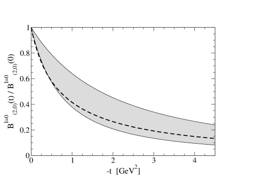
Figure 6: The same as in Fig. 5 but for the tensor GFF $B^{q}_{2,0}$(t).

Figure 7: The vector GFF $A^{q}_{2,0}(t)$, an isoscalar one, normalized to its own charge. Dashed line: CCQM result, corresponding to $m_{q}=~{}0.220$ GeV and $m_{R}=~{}1.192$ GeV in the vertex (56). The shaded area indicates the lattice data Bromth extrapolated to the pion physical mass $m_{\pi}=0.140$ GeV (see text).

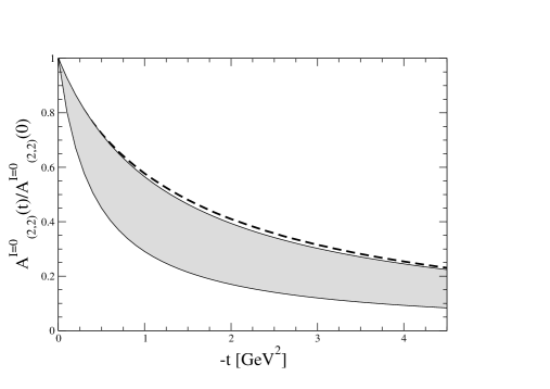
Figure 8: The same as in Fig. 7 but for the vector GFF $A^{q}_{2,2}$(t).

Table 6: Values at $t=0$ of the CCQM GFFs, $A^{q}_{2,0}(0)$, $A^{q}_{2,2}(0)$, $B^{q}_{1,0}(0)$ and $B^{q}_{2,0}(0)$.

$A^{q}_{2,0}(0)$	$A^{q}_{2,2}(0)$	$B^{q}_{1,0}(0)$	$B^{q}_{2,0}(0)$
0.4710	-0.03308	0.1612	0.05827

Table 7: GFFs for $t=0$ at a scale $\mu_{LAT}=2$ GeV. The first three rows contain the evolved (see text) CCQM results for $m_{q}=0.220$ GeV and $m_{R}=1.192$ GeV. The forth and fifth rows show the lattice extrapolations at the pion physical mass obtained in Refs. Bromth ; Brom08b and in Ref. Simula , respectively. The sixth and seventh rows present the calculations from the chiral quark model of Refs. Broni10 ; Aribron and from the instanton vacuum model of Ref. Nam11 , respectively. Notice that the results from Broni10 ; Aribron were not explicitly written in the works, so that they have been extrapolated by the plots presented there.

	$A^{q}_{2,0}(t=0,\mu=2~{}\textrm{GeV})$	$A^{q}_{2,2}(t=0,\mu=2~{}\textrm{GeV})$	$B^{q}_{1,0}(t=0,\mu=2~{}\textrm{GeV})$	$B^{q}_{2,0}(t=0,\mu=2~{}\textrm{GeV})$
CCQM
$\mu_{0}=0.496$	0.2485	-0.0175	0.1258	0.0277
$\mu_{0}=0.506$	0.2542	-0.0179	0.1269	0.0285
$\mu_{0}=0.549$	0.2752	-0.0193	0.1310	0.0313
Lattice
Ref. Bromth ; Brom08b	$0.261\pm 0.004$	$-0.066\pm 0.008$	$0.216\pm 0.034$	$0.039\pm 0.010$
Ref. Simula	-	-	$0.195\pm 0.010$	-
Chiral models
$\chi$QM Broni10 ; Aribron	$0.278\pm 0.015$	-	0.149	0.0287
IVM Nam11	-	-	0.216	0.032

If one is interested in a comparison that involves the full GFFs, then it is necessary to specify the scale and, accordingly, to evolve our CCQM results. In particular, since we have a multiplicative evolution, it is sufficient (i) to evolve only the value at $t=0$, namely the ones collected in Tab. 6, through Eqs. (100), (101), (102), (103), (5.4) and (5.4) and then (ii) to use Eq. (127). As in the case of the evolution of the PDF, we considered the three possible values of $\mu_{0}$ listed in Tab. 3. The results are shown in Tab. 7, together with lattice data Bromth ; Brom08b ; Simula and model calculations, obtained from a chiral quark model Broni10 ; Aribron and an instanton vacuum model Nam11 . It should be pointed out that within the chiral perturbation theory (see Ref. Dono91 ) one should have the following relation between the so-called gravitational FFs: $A^{q}_{22}(t)=-A^{q}_{20}(t)/4+{\cal O}(m^{2}_{\pi})$. This relation is verified by the lattice results, while CCQM does not. Moreover, one should observe that $A^{q}_{20}(0)$ slightly differs from $<x>$ at $\mu_{LAT}$ (see Tab. 2), that contains both quark and gluon contributions.

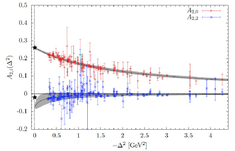
Figure 9: The lattice GFFs $A^{q}_{2,0}(t,\mu_{LAT})$ and $A^{q}_{2,2}(t,\mu_{LAT})$ of Ref. Bromth and the CCQM $A^{q}_{2,0}(t=0,\mu_{LAT})$ and $A^{q}_{2,2}(t=0,\mu_{LAT})$. Stars: CCQM result evolved at $\mu_{LAT}=~{}2$ GeV (the size of the symbols is roughly proportional to the uncertainties on CCQM initial scale $\mu_{CCQ}$). Shaded area: uncertainties of the fits to the lattice data, as estimated in Ref. Bromth (see text). (Adapted from Ref. Bromth ).

Figure 10: Comparison between the CCQM $B^{q}_{1,0}(t=0,\mu_{LAT})$ and $B^{q}_{2,0}(t=0,\mu_{LAT})$, divided by $m_{\pi}$ and the corresponding results from the chiral quark model of Ref. Broni10 and the lattice data of Ref. Brom08b . Stars: CCQM results evolved at $\mu_{LAT}=~{}2$ for $B^{q}_{1,0}(0)$ (upper one) and for $B^{q}_{2,0}(0)$ (lower one) (the size of the symbols is roughly proportional to the uncertainties on our initial scale $\mu_{CCQ}$ as illustrated in subsec. 5.1). Solid lines: results from the chiral quark model of Ref. Broni10 , vs $m^{2}_{\pi}$. Data points: lattice calculations from Ref. Brom08b . The vertical line corresponds to the physical pion mass. (Adapted from Ref. Broni10 ).

Figure 11: Comparison between the CCQM $B^{q}_{1,0}(0)$ evolved at $\mu_{LAT}=~{}2$ GeV and the lattice calculation from Ref. Simula . Circles: lattice data from Simula for different values of $m_{\pi}$. Square: extrapolation of the previous lattice data to the physical pion mass, $m_{\pi}^{phys}$, as it has been carried out in Ref. Simula . Triangle: CCQM result evolved at $\mu_{LAT}=~{}2$ GeV (the size of the symbols is roughly proportional to the uncertainties on our initial scale $\mu_{CCQ}$, as illustrated in subsec. 5.1). (Adapted from Ref. Simula ).

To have a better understanding of the quality of the comparison between our CCQM results and the lattice data shown in Tab. 7, we have added our calculation, at $t=0$, in Fig. 9, where the lattice results from Bromth , extrapolated at the physical pion mass, are presented for $A^{q}_{2,0}(t,\mu_{LAT})$ and $A^{q}_{2,2}(t,\mu_{LAT})$. In Fig. 9, the stars at $t=0$ represent the CCQM values evolved at the lattice scale (the size of the symbols is roughly proportional to the uncertainties of the initial $\mu_{CCQ}$ (cf subsec. 5.1), while the shaded area is the uncertainties produced by the fits to the lattice data, as elaborated in Ref. Bromth . It is clear that in order to have a conclusive comparison a more wide lattice data set is necessary, but on the other hand it is impressive that a small quantity, like $A^{q}_{2,2}(t,\mu_{LAT})$, can be extracted with a quite reasonable extent of reliability. In Figs. 10 and 11, analogous comparisons for $B^{q}_{1,0}(t=0,\mu_{LAT})$ and $B^{q}_{2,0}(t=0,\mu_{LAT})$ are shown. In particular, Fig. 10 contains both $B_{1,0}(t=0,\mu_{LAT})$ and $B^{q}_{2,0}(t=0,\mu_{LAT})$, evaluated within CCQM (stars) and within the chiral quark model of Ref. Broni10 with different $m_{\pi}$. In the figure the lattice data of Ref. Brom08b are also present. Again, the comparison between values at $t=0$ and physical pion mass appears non trivial. In Fig. 11, a recent lattice calculation of $B^{q}_{1,0}(t=0,\mu_{LAT})$ Simula is compared with our CCQM (triangles). In general, one has an overall agreement, a little bit better for $B^{q}_{2,0}(0)$.

The knowledge of GFFs allows one to investigate the probability density $\rho_{n}({\bf b}_{\perp},{\bf s}_{\perp})$ for a transversely-polarized u-quark (cf Eq. (32)). In particular, one can address the 3D structure of the pion in the impact parameter space. For instance, one can calculate the average transverse shifts when the quark is polarized along the $x$-axis, i.e. ${\bf s}_{\perp}\equiv\{1,0\}$. The shift for a given $n$ is given by Brom08b

$$\langle b_{y}\rangle_{n}={\int d{\bf b}_{\perp}~{}b_{y}~{}\rho_{n}({\bf b}_{\perp},{\bf s}_{\perp})\over\int d{\bf b}_{\perp}~{}\rho_{n}({\bf b}_{\perp},{\bf s}_{\perp})}={1\over 2m_{\pi}}~{}{B^{q}_{n,0}(t=0)\over A^{q}_{n,0}(t=0)}$$

(129)

From the CCQM values evolved at $\mu_{LAT}$, shown in Tab. 7, one can construct the shifts for $n=1,2$, and then compare with the corresponding lattice results, as given in Ref. Brom08b . In Tab. 8, the comparison is shown (recall that $A^{q}_{1,0}(t=0)=1$). Obviously, the same observations relevant for Tab. 7 can be also repeated for Tab. 8, since it contains the same information but presented in a different context.

Table 8: Mean shifts along the direction perpendicular to the u-quark transverse polarization, ${\bf s}_{\perp}\equiv\{1,0\}$, for $n=1,2$ (cf Eq. (129)). The CCQM results have been constructed from the values in Tab. 7 (notice that the uncertainties are originated by the three values listed there).

	CCQM - $m_{\pi}=140$ MeV	lattice Brom08b	lattice Simula
$\langle b_{y}\rangle_{1}$	0.0901 $\pm$ 0.0015  fm	0.151 $\pm$ 0.024  fm	0.137 $\pm$ 0.007  fm
$\langle b_{y}\rangle_{2}$	0.0796 $\pm$ 0.001  fm	0.106 $\pm$ 0.028  fm

The values shown in Tab. 8 indicate that even the simple version of a CCQM is able to reproduce a distortion of the transverse density in a direction perpendicular to the quark polarization, and in turn demonstrate the presence of a non trivial correlation between the orbital angular momenta and the spin of the constituents inside a pseudoscalar hadron, that attracts a great interest from both experimental and theoretical side (see, e.g., Bur05 ).

6 Conclusions

A simple, but fully covariant constituent quark model has been exploited for investigating the phenomenology of the leading-order Generalized Parton Distributions of the pion. The main ingredients of the approach are (i) the generalization of the Mandelstam formula, applied in the seminal work of Ref. Mandel to matrix elements of the em current operator between states of a relativistic composite system, and (ii) an Ansatz of the Bethe-Salpeter amplitude for describing the quark-pion vertex. Their combination produces a very effective tool that allows a careful phenomenological investigation of the pion, as shown in detail through the evaluation of both vector and tensor pion GPDs. We have also taken into account, at the leading order, the evolution for obtaining a meaningful comparison with both experimental data (see Fig. 2 for the comparison with the PDF extracted from the Drell-Yan data in Ref. Conway ) and lattice calculations of generalized form factors.

Summarizing, the CCQM proves to be quite satisfactory in describing the pion phenomenology, especially considering that the model involves relatively simple calculations and actually admits only one really free parameter (the mass $m_{q}$ of the constituent quark, since $m_{R}$ is constrained by $f_{\pi}$). It is worth noting that the CCQM is elaborated in Minkowski space, and the overall agreement we have shown with the lattice data, obtained in Euclidean space, could be an interesting source of information on the interplay of calculations performed in the two spaces, with a particular attention to the issue of the analytic behavior. In the future the present model could be substantially improved by enriching the analytic structure of the pion BS amplitude through a dynamical approach based on the solution of the BSE via the Nakanishi integral representation Naka (cf subsect 3.2), supplemented with a phenomenological kernel. In perspective, given the simplicity and the effectiveness of the approach, one could aim at applying the same model to more complex hadrons than the pion, e.g. to the nucleon within a quark-diquark framework.

References

- (1) P.A.M. Dirac, Forms of relativistic dynamics. Rev. Mod. Phys. 21, 392 (1949)
- (2) S. Brodsky, H-C Pauli, S. Pinsky, Quantum Chromodynamics and Other Field Theories on the Light Cone. Phys. Rep. 301, 299 (1998)
- (3) T. Frederico, E. Pace, B. Pasquini, and G. Salmè, Pion generalized parton distributions with covariant and light-front constituent quark models. Phys. Rev. D 80, 054021 (2009)
- (4) T. Frederico, E. Pace, B. Pasquini, and G. Salmè, Generalized parton distributions of the pion in a covariant Bethe-Salpeter model and light-front models. Nucl. Phys. B (Proc. Suppl.) 199, 264 (2010)
- (5) M. Diehl, Generalized parton distributions. Phys. Rep. 388, 41 (2003)
- (6) V. Barone, A. Drago, P. G. Ratcliffe, Transverse polarisation of quarks in hadrons. Phys. Rep. 359, 1 (2002)
- (7) S. Mandelstam, Dynamical variables in the Bethe-Salpeter formalism. Proc. Royal Soc. A 233, 248 (1956)
- (8) E. Pace, G. Romanelli and G. Salmè, Pion Tensor Generalized Parton Distributions in a Covariant Constituent Quark Model. Few-Body Syst. 52, 301 (2012).
- (9) E. Pace, G. Romanelli and G. Salmè, Exploring the Pion phenomenology within a fully covariant constituent quark model, Few-Body Syst. 54, 769 (2013)
- (10) M. Miyama and S. Kumano, Numerical solution of evolution equations in a brute-force method. Comput. Phys. Commun. 94, 185 (1996)
- (11) J.S. Conway et al., Experimental study of muon pairs produced by 252-GeV pions on tungsten. Phys. Rev. D 39, 92 (1989)
- (12) K. Wijesooriya, P. E. Reimer, and R. J. Holt, Pion parton distribution function in the valence region. Phys. Rev. C 72, 065203 (2005)
- (13) D. Brömmel, Pion structure from the lattice. Report No. DESY-THESYS-2007-023, 2007
- (14) D. Brömmel, et al (QCDSF/UKQCD Coll.), Quark distributions in the pion. PoS (LATTICE 2007) 140 (2008)
- (15) D. Brommel et al., Transverse spin structure of hadrons from lattice QCD. Prog. Part. Nucl. Phys. 61, 73 (2008)
- (16) D. Brommel et al., Spin Structure of the pion. Phys. Rev. Lett. 101, 122001 (2008)
- (17) S. Meißner, A. Metz, M. Schlegel, K. Goeke, Generalized parton correlation functions for a spin-0 hadron. JHEP 0808, 038 (2008).
- (18) Ph. Hägler, Hadron structure from lattice quantum Chromodynamics. Phys. Rep. 490, 49 (2010)
- (19) M. Burkardt, Impact parameter dependent parton distributions and transverse single spin asymmetries. Phys. Rev. D 72, 094020 (2005) Phys. Rev. D 66, 114005 (2002)
- (20) M. Burkardt, Transverse deformation of parton distributions and transversity decomposition of angular momentum. Phys. Rev. D 72, 094020 (2005)
- (21) M. Burkardt and B. Hannafious, Are all Boer-Mulders functions alike? Phys. Lett. B 658, 130 (2008)
- (22) M. Diehl and Ph. Hägler, Spin densities in the transverse plane and generalized transversity distributions. Eur. Phys. J. C 44, 87 (2005)
- (23) D. Brömmel et al., The pion form factor from lattice QCD with two dynamical flavors. Eur. Phys. J. C 51, 335(2007)
- (24) D. Boer and P. J. Mulders, Time-reversal odd distribution functions in leptoproduction. Phys. Rev. D 57, 5780 (1998)
- (25) Zhun Lü and Bo-Qiang Ma, Nonzero transversity distribution of the pion in a quark-spectator-antiquark model. Phys. Rev. D 70, 094044 (2004)
- (26) A.V. Belitsky, X. Ji and F. Yuan, Final state interactions and gauge invariant parton distribution. Nucl. Phys. B 656, 165 (2003)
- (27) P. Maris and C. D. Roberts, and K-meson Bethe-Salpeter amplitudes. Phys. Rev. C 56, 3369 (1997)
- (28) C. Itzykson and J. B. Zuber, Quantum Field Theory, Dover Pubns., Mineola, NY, 2005
- (29) J.P.B.C. de Melo, T. Frederico, E. Pace and G. Salmè, Pair term in the electromagnetic current within the Front-Form dynamics: spin-0 case. Nucl. Phys. A 707, 399 (2002)
- (30) J.P.B.C. de Melo, T. Frederico, E. Pace and G. Salmè, Electromagnetic form-factor of the pion in the space and time - like regions within the Front-Form dynamics. Phys. Lett. B 581, 75 (2004)
- (31) J.P.B.C. de Melo, T. Frederico, E. Pace and G. Salmè, Spacelike and timelike pion electromagnetic form-factor and Fock state components within the light-front dynamics. Phys. Rev. D 73, 074013 (2006)
- (32) J.P.B.C. de Melo, T. Frederico, E. Pace, G. Salmè and S. Pisano, Timelike and spacelike nucleon electromagnetic form factors beyond relativistic constituent quark models. Phys. Lett. B 671,153 (2009)
- (33) V. N. Gribov, L. N. Lipatov, Deep inelastic e-p scattering in perturbation theory. Sov. J. Nucl. Phys. 15, 438 (1972) [Yad. Fiz. 15, 781 (1972)]; e+ e- pair annihilation and deep inelastic e p scattering in perturbation theory. 15, 675 (1972)
- (34) G. Altarelli, G. Parisi, Asymptotic freedom in parton language. Nucl. Phys. B 126, 298 (1977)
- (35) Yu. L. Dokshitzer, Calculation of the Structure Functions for Deep Inelastic Scattering and e+ e- Annihilation by Perturbation Theory in Quantum Chromodynamics. Sov. Phys. JETP 46, 641 (1977)
- (36) A. V. Efremov, A. V. Radyushkin, Asymptotic behavior of the pion form factor in quantum chromodynamics. Phys. Lett. B 94, 245 (1980).
- (37) G. P. Lepage, S. J. Brodsky, Exclusive processes in perturbative quantum chromodynamics. Phys. Rev. D 22, 2157 (1980)
- (38) R.J. Holt and C.D. Roberts, Nucleon and pion distribution functions in the valence region. Rev. Mod. Phys. 82, 2991 (2010)
- (39) E. P. Biernat, F. Gross, M. T. Peña, and A. Stadler, Pion electromagnetic form factor in the covariant spectator theory. Phys. Rev. D 89, 016006 (2014)
- (40) N. Nakanishi, Graph Theory and Feynman Integrals, Gordon and Breach, New York, 1971.
- (41) J. Carbonell and V.A. Karmanov, Solving Bethe-Salpeter equation in Minkowski space. Eur. Phys. J. A 27, 1 (2006)
- (42) J. Carbonell and V.A. Karmanov, Solving the Bethe-Salpeter equation for two fermions in Minkowski space. Eur. Phys. J. A 46, 387 (2010)
-
(43)
T. Frederico, G. Salmè and M. Viviani,
Two-body scattering states in Minkowski
space and the Nakanishi integral representation onto the null plane. Phys. Rev.
D 85, 036009 (2012)
and
arXiv:1112.5568. - (44) T. Frederico, G. Salmè and M. Viviani, Quantitative studies of the homogeneous Bethe-Salpeter equation in Minkowski space. Phys. Rev. D 89, 016010 (2014).
- (45) T. Frederico, G. Salmè and M. Viviani, Solving the inhomogeneous Bethe-Salpeter Equation in Minkowski space: the zero-energy limit. Eur. Phys. J. C 75, 398 (2015).
- (46) S. M. Dorkin, M. Beyer, S.S. Semikh and L.P. Kaptari, Two-fermion bound states within the Bethe-Salpeter approach. Few-Body Syst. 42, 1 (2008)
- (47) S. M. Dorkin, L.P. Kaptari, B. Kämpfer, Accounting for the analytical properties of the quark propagator from the Dyson-Schwinger equation. Phys. Rev. C 91, 055201 (2015).
- (48) W. Greiner and A. Schäffer. Quantum Chromo Dynamics, Springer-Verlag, Berlin (1995)
- (49) A.V. Belisky and A.V. Radyushkin, Unraveling hadron structure with generalized parton distributions. Phys. Rep. 418, 1 (2005).
- (50) A.D. Martin et al., Parton distributions for the LHC. Eur. Phys. J. C 63, 189 (2009)
- (51) X. Ji, Deeply virtual Compton scattering. Phys. Rev. D 55, 7114 (1997)
- (52) P. Hoodbhoy and X. Ji, Helicity-flip off-forward parton distributions of the nucleon. Phys. Rev. D 58, 054006 (1998).
- (53) W. Broniowski, E.R. Arriola and K. Golec-Biernat, Generalized parton distributions of the pion in chiral quark models and their QCD evolution. Phys. Rev. D 77, 034023 (208)
- (54) W. Broniowski and E.R. Arriola, Note on the QCD evolution of generalized form factors. Phys. Rev. D 79, 057501 (2009).
- (55) N. Kivel and L. Mankiewicz, Conformal string operators and evolution of skewed parton distributions. Nucl. Phys. B 557, 271 (1999).
- (56) M. Kirch, A. Manashov and A. Schäfer, Evolution equation for generalized parton distributions. Phys. Rev. D 72, 114006 (2005).
- (57) W. Broniowski, A.E. Dorokhov, E.R. Arriola, Transversity form factors of the pion in chiral quark models. Phys. Rev. D 82, 094001 (2010)
- (58) A. E. Dorokhov, W. Broniowski and E. R. Arriola, Generalized quark transversity distribution of the pion in chiral quark models. Phys. Rev. D 84, 074015 (2011)
- (59) S. Nam and H.C. Kim, Spin structure of the pion from the instanton vacuum. Phys. Lett. B 700, 305 (2011)
- (60) K.A. Olive et al., Particle Data group. Chin. Phys. C 38, 090001 (2014)
- (61) BaBar Collaboration, B. Aubert et al., Measurement of the transition form factor. Phys. Rev. D 80, 052002 (2009)
- (62) Belle Collaboration, S. Uehara et al., Measurement of transition form factor at Belle. Phys. Rev. D 86, 092007 (2012)
- (63) S.J. Brodsky, F.-G. Cao and G. F. de Téramond, Evolved QCD predictions for the meson-photon transition form factors. Phys. Rev. D 84, 033001 (2011)
- (64) G. P. Lepage and S. J. Brodsky, Exclusive Processes in Perturbative Quantum Chromodynamics. Phys. Rev. D 22, 2157 (1980)
- (65) S.J. Brodsky and G.P. Lepage, Large-angle two-photon exclusive channels in quantum chromodynamics. Phys. Rev. D 24, 1808 (1981)
- (66) T. D. Rae, Moments of parton distribution amplitudes and structure functions for the light mesons from lattice QCD. ePrint ID: 199359 (2011), http://eprints.soton.ac.uk.
- (67) S. Capitani, et al ( Coll.), Parton distribution functions with twisted mass fermions. Phys. Lett. B 639, 520 (2006)
- (68) M. Guagnelli et al (ZeRo Coll.), Non-perturbative pion matrix element of a twist-2 operator from the lattice. Eur. Phys. J. C 40 69 (2005)
- (69) A. Abdel-Rehim et al (ETMC Coll.), Nucleon and pion structure with lattice QCD simulations at physical value of the pion. Phys. Rev. D 92, 114513 (2015)
- (70) W. J. Marciano, Flavor thresholds and in the modified minimal-subtraction scheme. Phys. Rev. D 29, 580 (1984)
- (71) A.D. Martin, W.J. Stirling and R.S. Thorne, MRST partons generated in a fixed-flavor scheme. Phys. Lett. B 636, 259 (2006)
- (72) M.B. Hecht, C.D. Roberts and S.M. Schmidt, Valence-quark distributions in the pion. Phys. Rev. C 63, 025213 (2001).
- (73) L. Chang et al, Basic features of the pion valence-quark distribution function. Phys. Lett. B 737, 23 (2014)
- (74) M. Aicher, A. Schäfer and W. Vogelsang, Soft-gluon resummation and valence parton distribution function of the pion. Phys. Rev. Lett. 105, 252003 (2010)
- (75) W. Broniowski and E. R. Arriola, Gravitational and higher-order form factors of the pion in chiral quark models. Phys. Rev. D 78, 094011 (2008)
- (76) W. Broniowski and E.R. Arriola, Application of chiral quarks to high-energy processes and lattice QCD. arXiv:0908.4165.
- (77) M. Diehl and L. Szymanowski, The transverse spin structure of the pion at short distances. Phys. Lett. B 690, 149 (2010)
- (78) I. Baum, V. Lubicz, G. Martinelli, L. Orifici, and S. Simula, Matrix elements of the electromagnetic operator between kaon and pion states. Phys. Rev. D 84, 074503 (2011)
- (79) J.F. Donoghue and H. Leutwyler, Energy and momentum in chiral theories. Z. Phys. C 52, 343 (1991)