Classification with Repulsion Tensors: A Case Study on Face Recognition

Abstract

We consider dimensionality reduction methods for face recognition in a supervised setting, using an image-as-matrix representation. A common procedure is to project image matrices into a smaller space in which the recognition is performed. These methods are often called “two-dimensional” in the literature and there exist counterparts that use an image-as-vector representation. When two face images are close to each other in the input space they may remain close after projection - but this is not desirable in the situation when these two images are from different classes, and this often affects the recognition performance. We extend a previously developed ‘repulsion Laplacean’ technique based on adding terms to the objective function with the goal or creation a repulsion energy between such images in the projected space. This scheme, which relies on a repulsion graph, is generic and can be incorporated into various two-dimensional methods. It can be regarded as a multilinear generalization of the repulsion strategy by Kokiopoulou and Saad [Pattern Recog., 42 (2009), pp. 2392–2402]. Experimental results demonstrate that the proposed methodology offers significant recognition improvement relative to the underlying two-dimensional methods.

1 Introduction

Numerous linear dimensionality reduction methods have been developed for classification tasks. Among these are a class methods which convert the data items to vectors in numerical form. For example, in face recognition, a face image is transformed into a column vector by concatenating rows or columns. A linear projector is obtained using the training data. The projector projects both training and test data into a lower dimensional space, in which the recognition task is performed. Typical examples of these include principal component analysis (PCA) [32, 31], linear discriminant analysis (LDA) [3, 5, 23], locality preserving projections (LPP) [9, 10], and neighborhood preserving projections (NPP) [8]. There are counterparts of LPP and NPP which enforce orthogonality constraint on the projector. They are denoted by OLPP and ONPP [14, 15], respectively.

Two-dimensional projection methods, treating each image as a matrix, with a goal of exploiting spatial redundancy. In the literature, such methods often utilize the key word ‘two-dimensional’ to charaterize them. They can be categorized into two different types. The first type of methods aim to preserve the distinct features of the data matrices in the projection [17, 29, 35, 36, 37]. These methods can be regarded as two-dimensional generalizations of the classical principal component analysis.

The other type of methods aim to preserve the closeness of neighboring data items in the projected space. In a supervised setting, two items are regarded as neighbors if they share the same class label. Examples of such methods include two-dimensional linear discriminant analysis (2D-LDA) [11, 20], two-dimensional neighborhood preserving projections (2D-NPP) [22, 26], and two-dimensional locality preserving projections (2D-LPP) [4, 7, 25].

Table 1: Linear dimensionality reduction methods.

Data	Method	Abbrev.	In Face Recog.	References
1D	Principal Component Analysis	PCA	Eigenfaces	[12, 32, 31]
	Linear Discriminant Analysis	LDA	Fisherfaces	[3, 5, 23]
	Locality Preserving Projections	LPP	Laplacianfaces	[9, 10]
	Neighborhood Preserving Projections	NPP	-	[8, 14, 15]
2D	Principal Component Analysis	2D-PCA	2D-Eigenfaces	[17, 29, 35, 36, 37]
	Linear Discriminant Analysis	2D-LDA	2D-Fisherfaces	[11, 21, 38]
	Locality Preserving Projections	2D-LPP	2D-Laplacianfaces	[4, 7, 25]
	Neighborhood Preserving Projections	2D-NPP	-	[26, 22]

The aforementioned methods are summarized in Table 1, where the synonyms in the application of face recognition, if any, are also listed.

An enhanced graph-based dimensionality reduction technique, repulsion Laplaceans [16], was proposed to improve the classification methods which use image-as-vector representation. The objective is to repel from other data points that are not from the same class but that close to each other in the input high-dimensional space.

In this paper, we develop a generalized methodology using repulsion tensors to improve the two-dimensional projection methods. This method is generic and can be applied to various methods, such as 2D-OLPP, 2D-ONPP, and 2D-LDA. The experiments on face recognition demonstrate significant improvements in the recognition performance over the existing two-dimensional methods. Compared to the peers using the image-as-vector representation, the proposed technique achieves substantial computational savings.

The rest of this paper is organized as follows. Section 2 formulates the two-dimensional projection methods in tensor form, establishes the connections between them, and gives a unified view. The enhancement with repulsion tensors is presented in Section 3, which also gives a unified framework for computing the projectors. Section 4 reports on experimental results with face recognition. The paper ends with conclusing remarks and a discussion of future work in Section 5. Appendix A introduces the concept of tensors and some related operations useful in this paper. Appendix B reviews the linear dimensionality reduction methods using image-as-vector representation.

The notational conventions in this paper are as follows. We denote scalars and vectors by lowercase letters (e.g., $m,n$), matrices by uppercase letters (e.g., $U,V$), and tensors by calligraphic letters (e.g., $\mathcal{A},\mathcal{B}$). An exception is that $I,J,K$ are used for upper bounds of indices. For a third order tensor $\mathcal{A}\in\mathbb{R}^{I\times J\times K}$, its $(i,j,k)$ entry is denoted by $a_{ijk}$. We also use MATLAB-like notation. For example, $\mathcal{A}(i,j,k)=a_{ijk}$, and $\mathcal{A}(:,:,k)$ is the matrix formed by elements $a_{ijk}$ for $i=1,\dots,I$ and $j=1,\dots,J$ and the specified $k$. We use $I_{n}$ to denote the identity matrix of size $n$-by-$n$, and $e_{n}$ to denote the vector of ones of length $n$. The norm $\|\cdot\|$ indicates the Frobenius norm.

2 Tensor formulation of 2D methods

Table 1 summarizes various known two-dimensional methods for image subspace analysis. These methods treat each image as a matrix $X_{k}\in R^{m_{1}\times m_{2}}$. The general form of the bilateral projection is

$$Y_{k}=U^{T}X_{k}V\in R^{d_{1}\times d_{2}},\quad k=1,\dots,n,$$ (1)

where $d_{1}\leq m_{1}$ and $d_{2}\leq m_{2}$. The transformation matrices $U$ and $V$ from the training data are applied to a test image $X$ to obtain a projected image $Y=U^{T}XV$, and the recognition is performed by comparing $Y$ to $Y_{1},\dots,Y_{n}$. When $U$ is an identity matrix ($d_{1}=m_{1}$) or $V$ is an identity matrix ($d_{2}=m_{2}$), the projection is said to be unilateral.

In this section, we formulate these methods in tensor form. Readers are referred to [1] for tensor concepts and operations. A brief introduction of the main ideas is also given in Appendix A.

Aggregating the matrices in (1), we obtain the third order tensors $\mathcal{X}\in\mathbb{R}^{m_{1}\times m_{2}\times n}$ and $\mathcal{Y}\in\mathbb{R}^{d_{1}\times d_{2}\times n}$, such that $\mathcal{X}(:,:,k)=X_{k}$ and $\mathcal{Y}(:,:,k)=Y_{k}$ for $k=1,\dots,n$. The relation between $\mathcal{X}$ and $\mathcal{Y}$ can be written succinctly as

$$\mathcal{Y}=\mathcal{X}\times_{1}U^{T}\times_{2}V^{T}.$$ (2)

Constraints should be imposed to the transformation matrices $U$ and $V$. A popular choice is the orthogonality

$$U^{T}U=I_{d_{1}},\quad V^{T}V=I_{d_{2}}.$$ (3)

To facilitate the discussion, we introduce the concept of tensor trace. Given a fourth order tensor $\mathcal{B}=[b_{ijkh}]\in\mathbb{R}^{I\times J\times I\times J}$, we define the tensor trace by

$$\mbox{tr}_{[1,2;3,4]}(\mathcal{B})=\sum_{i=1}^{I}\sum_{j=1}^{J}b_{ijij},$$ (4)

where the subscript $[1,2;3,4]$ specifies the order of the dimensions respect to which the trace is taken. This is a generalization of the trace of a square matrix. In this paper we always use the order $[1,2;3,4]$ in the tensor trace. Hence we abbreviate $\mbox{tr}_{[1,2;3,4]}(\mathcal{B})$ as $\mbox{tr}(\mathcal{B})$. A useful property which parallels the relation $\|A\|^{2}=\mbox{tr}(AA^{T})$ is

$$\|\mathcal{A}\|^{2}=\mbox{tr}(\langle\mathcal{A},\mathcal{A}\rangle_{[3;3]}),$$

where $\mathcal{A}=\mathbb{R}^{I\times J\times K}$ is a third order tensor, and $\langle\mathcal{A},\mathcal{A}\rangle_{[3;3]}$ is the mode-$[3;3]$ contracted tensor product. In the following discussion, we will use tensor and matrix notation interchangeably.

2.1 Two-dimensional PCA

We consider a class of tensor methods which can be regarded as high order generalizations of the classical PCA [17, 29, 35, 36, 37]. The discussion starts with a bilateral projection method, also referred to as the generalized low rank approximation of matrices (GLRAM) [37] or the concurrent subspaces analysis (CSA) [35]. This is a special case of the high order orthogonal iteration (HOOI) of tensors [19, 29].

The goal here is to find a reduced representation $Y_{k}\in\mathbb{R}^{d_{1}\times d_{2}}$ of each $X_{k}\in\mathbb{R}^{m_{1}\times m_{2}}$ for $k=1,\dots,n$. The reconstructed data, associated with two orthogonal matrices $U$ and $V$ ($U^{T}U=I_{d_{1}}$ and $V^{T}V=I_{d_{2}}$), is $\widehat{X}_{k}=UY_{k}V^{T}$. Each $\widehat{X}$ is a rank-$d$ approximation of $X$, where $d=\min\{d_{1},d_{2}\}$. The reconstruction errors are measured by

$$\sum_{k=1}^{n}\|X_{k}-\widehat{X}_{k}\|^{2}=\sum_{k=1}^{n}\|X_{k}-UY_{k}V^{T}\|^{2}$$ (5)

Now let $f_{k}(Y)=\|X_{k}-UYV^{T}\|^{2}$, which equals

$$\mbox{tr}(X_{k}X_{k}^{T})+\mbox{tr}(YY^{T})-2\,\mbox{tr}(YU^{T}X_{k}V).$$

Since $f_{k}(Y)$ is convex, the minimum of $f_{k}(Y)$ is achieved by setting $\nabla f_{k}=0$, from which we obtain $Y=U^{T}X_{k}V$. Therefore, when (5) is minimized, (1) is satisfied.

Substituting (1) into (5), we obtain

$$\sum_{k=1}^{n}\|X_{k}-UU^{T}X_{k}VV^{T}\|^{2}=\sum_{k=1}^{n}\|X_{k}\|^{2}-\|U^{T}X_{k}V\|^{2}=\|\mathcal{X}\|^{2}-\|\mathcal{X}\times_{1}U^{T}\times_{2}V^{T}\|^{2}.$$

As a result, minimizing $\|\mathcal{X}-\mathcal{Y}\times_{1}U\times_{2}V\|^{2}$ is equivalent to maximizing $\|\mathcal{X}\times_{1}U^{T}\times_{2}V^{T}\|^{2}$. We end-up with the following problem:

$$\left\{\begin{array}[]{ll}\displaystyle\mathop{\mbox{maximize}}_{U,\,V}&\|\mathcal{X}\times_{1}U^{T}\times_{2}V^{T}\|^{2}\\ \textup{subject to}&U^{T}U=I_{d_{1}},\;V^{T}V=I_{d_{2}}.\end{array}\right.$$ (6)

Note that we can write $\|\mathcal{X}\times_{1}U^{T}\times_{2}V^{T}\|^{2}$ in tensor trace form as

$$\mbox{tr}(\langle\mathcal{X}\times_{1}U^{T}\times_{2}V^{T},\mathcal{X}\times_{1}U^{T}\times_{2}V^{T}\rangle_{[3;3]}).$$ (7)

A variant of the above method is called the generalized two-dimensional PCA [17]. The formulation is essentially the same as (6), except that before dimensionality reduction, the data matrices are rigidly translated so that its centroid is at the origin. To be specific, the translated matrices are $\widetilde{X}_{k}=X_{k}-\bar{X}$ for $i=1,\dots,n$, where $\bar{X}=\frac{1}{n}\sum_{i=1}^{n}X_{i}$ is the centroid matrix. Let $\widetilde{\mathcal{X}}$ be the translated tensor such that $\widetilde{\mathcal{X}}(:,:,k)=\widetilde{X}_{k}$ for $k=1,\dots,n$. Then

$$\widetilde{\mathcal{X}}=\mathcal{X}-\mathcal{X}\times_{3}\frac{e_{n}^{T}}{n}\times_{3}e_{n}=\mathcal{X}-\mathcal{X}\times_{3}(\frac{e_{n}e_{n}^{T}}{n})=\mathcal{X}\times_{3}(I_{n}-\frac{1}{n}e_{n}e_{n}^{T}),$$

where $e_{n}\in\mathbb{R}^{n}$ is the column vector of ones. In a similar discussion leading to (6), we obtain the program

$$\left\{\begin{array}[]{ll}\displaystyle\mathop{\mbox{maximize}}_{U,V}&\|\mathcal{X}\times_{1}U^{T}\times_{2}V^{T}\times_{3}J_{n}\|^{2}\\ \textup{subject to}&U^{T}U=I_{d_{1}},\;V^{T}V=I_{d_{2}},\end{array}\right.$$ (8)

where $J_{n}=I_{n}-\frac{1}{n}e_{n}e_{n}^{T}$ is the centering matrix. The objective function can be written in the form of tensor trace as

$$\mbox{tr}(\mathcal{X}\times_{1}U^{T}\times_{2}V^{T}\times_{3}J_{n},\mathcal{X}\times_{1}U^{T}\times_{2}V^{T}).$$ (9)

Note that $J_{n}$ is a projection matrix. Hence $J_{n}^{2}=J_{n}=J_{n}^{T}$. This property has been used in deriving (9). We call the dimensionality reduction method which solves (8) the 2D-PCA hereafter.

There is no closed form of solution to (6) and (8). One can use the high order orthogonal iteration (HOOI) [19] to compute $U$ and $V$.

One may perform 2D-PCA with the projection applied to only one side of the input image matrices [36]. For example, we set $V$ as the identity $I_{m_{2}}$ and therefore the projection is in the form $Y_{i}=U^{T}X_{i}\in\mathbb{R}^{d_{1}\times m_{2}}$ for $i=1,\dots,n$. This unilateral projection is equivalent to performing PCA on the columns of all images.

2.1.1 Connection to PCA

Recall that PCA maximizes the trace of covariance matrix of the embedded data subject to orthogonal projection. See, e.g., Appendix B.1. Now we draw the corresponding property of 2D-PCA. Substituting (2) into the objective function of (8), we obtain

$$\|\mathcal{Y}\times_{3}J_{n}\|^{2}=\sum_{k=1}^{n}\|Y_{k}-\bar{Y}\|^{2}=\mbox{tr}\left[\sum_{k=1}^{n}(Y_{k}-\bar{Y})(Y_{k}-\bar{Y})^{T}\right],$$

where $\bar{Y}=\sum_{k=1}^{n}Y_{k}$. Here

$$\frac{1}{n}\sum_{k=1}^{n}(Y_{k}-\bar{Y})(Y_{k}-\bar{Y})^{T}$$

is called the image covariance matrix, whose trace is maximized by 2D-PCA subject to the orthogonality constraints (3). If $m_{2}=1$, then $Y_{1},\dots,Y_{n}$ are indeed column vectors, in which case 2D-PCA is equivalent to PCA.

2.2 Two-dimensional LPP

LPP and OLPP, reviewed in Appendix B.3, are linear dimensionality reduction methods using image-as-vector representation. Their two-dimensional counterparts, using image-as-matrix representation [4, 7, 25], are presented next.

The step to construct the symmetric weight matrix $W=[w_{ij}]\in\mathbb{R}^{n\times n}$ is the same as that in LPP and OLPP. We also compute the graph Laplacian $L=D-W$, where $D\in\mathbb{R}^{n\times n}$ is the diagonal matrix formed by elements $d_{ii}=\sum_{j=1}^{n}w_{ij}$ for $i=1,\dots,n$. See Appendix B.2 for details.

LPP and OLPP minimize the objective function (56) in Appendix B.4. Correspondingly, we minimize

$$\frac{1}{2}\sum_{i,j=1}^{n}w_{ij}\|Y_{i}-Y_{j}\|^{2} = \frac{1}{2}\sum_{i,j=1}^{n}\mbox{tr}\left[w_{ij}(Y_{i}-Y_{j})(Y_{i}-Y_{j})^{T}\right]$$

$$= \mbox{tr}\left[\sum_{i=1}^{n}d_{ii}Y_{i}Y_{i}^{T}-\sum_{i,j=1}^{n}w_{ij}Y_{i}Y_{j}^{T}\right]$$

$$= \mbox{tr}\left[\sum_{k=1}^{d_{2}}\sum_{i=1}^{n}d_{ii}\mathcal{Y}(:,k,i)\mathcal{Y}(:,k,i)^{T}\right.\left.-\sum_{k=1}^{d_{2}}\sum_{i,j=1}^{n}w_{ij}\mathcal{Y}(:,k,i)\mathcal{Y}(:,k,j)^{T}\right]$$

$$= \mbox{tr}\left[\sum_{k=1}^{d_{2}}\mathcal{Y}(:,k,:)(D-W)\mathcal{Y}(:,k,:)^{T}\right]$$

$$= \sum_{k=1}^{d_{2}}\mbox{tr}\left[\mathcal{Y}(:,k,:)L\mathcal{Y}(:,k,:)^{T}\right]$$

$$= \mbox{tr}(\langle\mathcal{Y}\times_{3}L,\mathcal{Y}\rangle_{[3;3]}),$$ (11)

where the tensor trace in (11) is defined in (4). Note that the last term (11) is a tensor generalization of $\mbox{tr}(YLY^{T})$ in (56).

We can substitute (2) into (11) and obtain

$$\mbox{tr}(\langle\mathcal{X}\times_{1}U^{T}\times_{2}V^{T}\times_{3}L,\mathcal{X}\times_{1}U^{T}\times_{2}V^{T}\rangle_{[3;3]}).$$ (12)

Constraints are required in the minimization of (12). For example, we can impose the orthogonality $U^{T}U=I_{d_{1}}$ and $V^{T}V=I_{d_{2}}$ in (3). This option leads to the 2D-OLPP method,

$$\left\{\begin{array}[]{ll}\displaystyle\mathop{\mbox{minimize}}_{U,V}&\displaystyle\mbox{tr}(\langle\mathcal{Y}\times_{3}L,\mathcal{Y}\rangle_{[3;3]})\\ \textup{subject to}&\mathcal{Y}=\mathcal{X}\times_{1}U\times_{2}V,\\ &U^{T}U=I_{d_{1}},\;V^{T}V=I_{d_{2}}.\end{array}\right.$$ (13)

How to solve this optimization problem (13) will be discussed in a unified framework in Section 3.3.

Alternatively, we may consider concurrently maximizing

$$\mbox{tr}(\langle\mathcal{X}\times_{1}U^{T}\times_{2}V^{T}\times_{3}D,\mathcal{X}\times_{1}U^{T}\times_{2}V^{T}\rangle_{[3;3]}),$$ (14)

which corresponds to $\mbox{tr}(YDY^{T})$ in the LPP program (54). Minimizing the ratio of (12) to (14) subject to $U^{T}U=I_{d_{1}}$ and $V^{T}V=I_{d_{2}}$ is a tensor generalization of the trace ratio optimization problem [24, 34]. Rather than solving this challenging problem, we will give a workaround in a unified framework in Section 3.3. This corresponds to the alternating algorithm in [7]. We call the resulting method 2D-LPP.

When $m_{2}=1$, $X_{1},\dots,X_{n}$ are indeed column vectors, and the data tensor $\mathcal{X}$ can be represented by a matrix $[X_{1},\dots,X_{n}]$, in which case 2D-LPP is reduced to the formulation of LPP (54), and 2D-OLPP is equivalent to OLPP.

2.3 Two-dimensional NPP

Recall that NPP and ONPP, reviewed in Appendix B.4, are linear dimensionality reduction methods that use the image-as-vector representation. Here we present their two-dimensional counterparts, using the image-as-matrix representation [22, 26].

Firstly, we compute a weight matrix $W=[w_{ij}]\in\mathbb{R}^{n\times n}$ in the same way as that of NPP and ONPP. See Appendix B.2 for a discussion. Then we consider the objective function to minimize

$$\sum_{i=1}^{n}\|Y_{i}-\sum_{j=1}^{n}w_{ij}Y_{j}\|^{2} = \sum_{i=1}^{n}\|\mathcal{Y}(:,:,i)-\sum_{j=1}^{n}w_{ij}\mathcal{Y}(:,:,j)\|^{2}$$

$$= \sum_{k=1}^{d_{2}}\sum_{i=1}^{n}\|\mathcal{Y}(:,k,i)-\sum_{j=1}^{n}w_{ij}\mathcal{Y}(:,k,j)\|^{2}$$

$$= \sum_{k=1}^{d_{2}}\|\mathcal{Y}(:,k,:)-\mathcal{Y}(:,k,:)\times_{3}W\|^{2}$$

$$= \sum_{k=1}^{d_{2}}\|\mathcal{Y}(:,k,:)\times_{3}(I_{n}-W)\|^{2}$$

$$= \|\mathcal{Y}\times_{3}(I_{n}-W)\|^{2},$$ (16)

which parallels the objective function of NPP and ONPP (56).

To match the format of (11), we rewrite (16) in the tensor trace form as

$$\mbox{tr}(\langle\mathcal{Y}\times_{3}H,\mathcal{Y}\rangle_{[3;3]}),$$ (17)

where $H=(I_{n}-W)^{T}(I_{n}-W)$. We can further substitute (2) into (17) and obtain

$$\mbox{tr}(\langle\mathcal{X}\times_{1}U^{T}\times_{2}V^{T}\times_{3}H,\mathcal{X}\times_{1}U^{T}\times_{2}V^{T}\rangle_{[3;3]}).$$ (18)

Again, one can impose the orthogonality constraints $U^{T}U=I_{d_{1}}$ and $V^{T}V=I_{d_{2}}$, yielding the 2D-ONPP method. Another option is to concurrently maximizing

$$\|\mathcal{X}\times_{1}U^{T}\times_{2}V^{T}\|^{2}.$$ (19)

We would like to write (19) in tensor trace form as

$$\mbox{tr}(\langle\mathcal{X}\times_{1}U^{T}\times_{2}V^{T},\mathcal{X}\times_{1}U^{T}\times_{2}V^{T}\rangle_{[3;3]}),$$ (20)

which is same as the objective function of GLRAM and CSA (7).

Minimizing the ratio (18) to (20) subject to $U^{T}U=I_{d_{1}}$ and $V^{T}V=I_{d_{2}}$ is a challenging tensor trace ratio optimization problem. A workaround will be given in the unified framework in Section 3.3. This corresponds to the alternating algorithm in [22]. The resulting method is called 2D-NPP.

Note that if $m_{2}=1$, then $X_{1},\dots,X_{n}$ are indeed column vectors, and the data tensor $\mathcal{X}$ can be represented by a matrix $[X_{1},\dots,X_{n}]$, in which case 2D-NPP and 2D-ONPP are reduced to the formulations of NPP (57) and ONPP (58), respectively.

2.3.1 Connection to 2D-PCA

Comparing the 2D-ONPP method to the 2D-PCA program (8), there are only two differences. Firstly, 2D-ONPP ‘minimizes’ (18), whereas 2D-PCA ‘maximizes’ (9). Both impose the orthogonality constraints $U^{T}U=I_{d_{1}}$ and $V^{T}V=I_{d_{2}}$. Secondly, the multiplication $\times_{3}(I_{n}-\frac{1}{n}e_{n}e_{n}^{T})$ in (9) corresponds to the multiplication $\times_{3}(I_{n}-W)$ in (18). If a complete graph is used and the weights are uniformly distributed, then $w_{ij}=\frac{1}{n}$ for $i,j=1,\dots,n$, yielding $W=\frac{1}{n}e_{n}e_{n}^{T}$. In this case, the objective functions of 2D-PCA and 2D-ONPP are identical. This is a property similar to the connection between PCA and ONPP [14, 15].

2.4 Two-dimensional LDA

We now present the two-dimensional counterpart of LDA [38], using image-as-matrix representation instead of image-as-vector representation.

Suppose we are given training data matrices $X_{1},\dots,X_{n}\in\mathbb{R}^{m_{1}\times m_{2}}$. Each data sample $X_{i}$ is associated with a class label $c(i)$. For each class $j=1,\dots,c$, there is an index set

$$\mathcal{C}_{j}=\{i:c(i)=j\},$$

whose size is denoted by $n_{j}=|\mathcal{C}_{j}|$.

The reduced data is obtained from the bilateral transformation $Y_{k}=U^{T}X_{k}V$ for $k=1,\dots,n$. The mean of each class $j$ is denoted by $\bar{Y}_{j}=\frac{1}{n_{j}}\sum_{i\in\mathcal{C}_{j}}Y_{i}$, and the global mean is $\bar{Y}=\frac{1}{n}\sum_{i=1}^{n}Y_{i}$. The within-scatter measure is defined by

$$D_{w}=\mbox{tr}(\sum_{j=1}^{c}\sum_{i\in\mathcal{C}_{j}}(Y_{i}-\bar{Y}_{j})(Y_{i}-\bar{Y}_{j})^{T}),$$ (21)

and the between-scatter measure is

$$D_{b}=\mbox{tr}(\sum_{j=1}^{c}n_{j}(\bar{Y}-\bar{Y}_{j})(\bar{Y}-\bar{Y}_{j})^{T}).$$ (22)

Note that if $m_{2}=1$, then $X_{1},\dots,X_{n}$ are indeed column vectors and the data tensor $\mathcal{X}$ can be represented by a matrix $[X_{1},\dots,X_{n}]$, in which case $D_{w}$ in (21) and $D_{b}$ in (22) are the same as $\mbox{tr}(U^{T}S_{w}U)$ and $\mbox{tr}(U^{T}S_{b}U)$ in LDA, where $S_{w}$ and $S_{b}$ are defined in (59) and (60), respectively. Conceptually, the goal is to minimize $D_{w}$ and maximize $D_{b}$, corresponding to minimizing $\mbox{tr}(U^{T}S_{w}U)$ and maximizing $\mbox{tr}(U^{T}S_{b}U)$ in LDA.

To write (21) and (22) in the tensor trace form, we aggregate $Y_{1},\dots,Y_{n}$ to form a data tensor $\mathcal{Y}$ such that $\mathcal{Y}(:,:,k)=Y_{k}$. For each class $j$, we form a data tensor $\mathcal{Y}_{j}$ to store all $Y_{i}$ with $c(i)=j$. In MATLAB-like notation, $\mathcal{Y}_{j}=\mathcal{Y}(:,:,c(i)==j).$ We also define a corresponding translated data tensor $\widetilde{\mathcal{Y}}_{j}$ by $\widetilde{\mathcal{Y}}_{j}(:,:,k)=\mathcal{Y}_{j}(:,:,k)-\bar{Y}_{j}$ for $k=1,\dots,n_{j}$. The relation between $\widetilde{\mathcal{Y}}_{j}$ and $\mathcal{Y}_{j}$ can be written as

$$\widetilde{\mathcal{Y}}_{j}=\mathcal{Y}_{j}-\mathcal{Y}_{j}\times_{3}\frac{e_{n_{j}}^{T}}{n_{j}}\times_{3}e_{n_{j}}=\mathcal{Y}-\mathcal{Y}\times_{3}(\frac{e_{n_{j}}e_{n_{j}}^{T}}{n_{j}})=\mathcal{Y}\times_{3}(I_{n_{j}}-\frac{1}{n_{j}}e_{n_{j}}e_{n_{j}}^{T}).$$

Hence we have

$$\mbox{tr}(\sum_{i\in\mathcal{C}_{j}}(Y_{i}-\bar{Y}_{j})(Y_{i}-\bar{Y}_{j})^{T})=\sum_{i\in\mathcal{C}_{j}}\|Y_{i}-\bar{Y}_{j}\|^{2}=\|\widetilde{\mathcal{Y}}_{j}\|^{2}=\mbox{tr}(\langle\widetilde{\mathcal{Y}}_{j},\widetilde{\mathcal{Y}}_{j}\rangle_{[3;3]})=\mbox{tr}(\langle\mathcal{Y}_{j}\times_{3}J_{n_{j}},\mathcal{Y}_{j}\rangle_{[3;3]}),$$

where $J_{n_{j}}=I_{n_{j}}-\frac{1}{n_{j}}e_{n_{j}}e_{n_{j}}^{T}$. Note that since $J_{n_{j}}$ is a projection matrix, $J_{n_{j}}^{T}=J_{n_{j}}=J_{n_{j}}^{2}$. This property has been used for the last equality.

Now we can rewrite (21) as

$$D_{w}=\sum_{j=1}^{c}\mbox{tr}(\sum_{i\in\mathcal{C}_{j}}(Y_{i}-\bar{Y}_{j})(Y_{i}-\bar{Y}_{j})^{T})=\sum_{j=1}^{c}\mbox{tr}(\langle\mathcal{Y}_{j}\times_{3}J_{n_{j}},\mathcal{Y}_{j}\rangle_{[3;3]})=\mbox{tr}(\langle\mathcal{Y}\times_{3}S,\mathcal{Y}\rangle_{[3;3]}),$$ (23)

where in MATLAB-like notation, $S(\mathcal{C}_{k},\mathcal{C}_{k})=J_{n_{k}}$ for $k=1,\dots,c$, and $S(i,j)=0$ if $c(i)\neq c(j)$. Substituting (2) into (23), we obtain the tensor trace form of $D_{w}$ as

$$D_{w}=\mbox{tr}(\langle\mathcal{X}\times_{1}U^{T}\times_{2}V^{T}\times_{3}S,\mathcal{X}\times_{1}U^{T}\times_{2}V^{T}\rangle_{[3;3]}).$$ (24)

The matrix $S$ actually is the Laplacian matrix of a label graph with even weights [25]. To be precise, let $W=I_{n}-S$ with $I_{n}\in\mathbb{R}^{n\times n}$ the identity. Then $W=[w_{ij}]\in\mathbb{R}^{n\times n}$ satisfies

$$w_{ij}=\left\{\begin{array}[]{ll}1/n_{k}&\mbox{if }c(i)=c(j);\\ 0&\mbox{otherwise}.\end{array}\right.$$ (25)

This matrix $S$ has rank $n-c$. See, for example, [10, 14, 15]. The discussion gives a connection to 2D-LPP.

Now we consider $D_{b}$ in (22), where

$$\sum_{j=1}^{c}n_{j}(\bar{Y}-\bar{Y}_{j})(\bar{Y}-\bar{Y}_{j})^{T} = (\sum_{j=1}^{c}n_{j})\bar{Y}\bar{Y}^{T}-(\sum_{j=1}^{c}n_{j}\bar{Y}_{j})\bar{Y}^{T}-\bar{Y}(\sum_{j=1}^{c}n_{j}\bar{Y}_{j})^{T}+\sum_{j=1}^{c}n_{j}\bar{Y}_{j}\bar{Y}_{j}^{T}$$

$$= -n\bar{Y}\bar{Y}^{T}+\sum_{j=1}^{c}n_{j}\bar{Y}_{j}\bar{Y}_{j}^{T}.$$

Hence we can rewrite (22) as

$$D_{b}=-n\,\mbox{tr}(\bar{Y}\bar{Y}^{T})+\sum_{j=1}^{c}n_{j}\mbox{tr}(\bar{Y}_{j}\bar{Y}_{j}^{T})=-n\|\bar{Y}\|^{2}+\sum_{j=1}^{c}n_{j}\|\bar{Y}_{j}\|^{2}.$$ (26)

The two terms in (26) can be written in tensor trace form as follows. First,

$$n\|\bar{Y}\|^{2}=n\|\mathcal{Y}\times_{3}\frac{e^{T}}{n}\|^{2}\\ =\mbox{tr}(\langle\mathcal{Y}\times_{3}\frac{e_{n}e_{n}^{T}}{n},\mathcal{Y}\rangle_{[3;3]}).$$

Then we have

$$\|\mathcal{Y}\|^{2}-n\|\bar{Y}\|^{2}=\mbox{tr}(\langle\mathcal{Y}\times_{3}J_{n},\mathcal{Y}\rangle_{[3;3]}),$$ (27)

where $J_{n}=I_{n}-\frac{e_{n}e_{n}^{T}}{n}$. Note that (27) is the same as the objective function (9) of 2D-PCA. Secondly,

$$\sum_{j=1}^{c}n_{j}\|\bar{Y}_{j}\|^{2}=\sum_{j=1}^{c}\mbox{tr}(\langle\mathcal{Y}_{j}\times_{3}\frac{e_{n_{j}}e_{n_{j}}^{T}}{n_{j}}),\mathcal{Y}\rangle_{[3;3]})=\mbox{tr}(\langle\mathcal{Y}\times_{3}W,\mathcal{Y}\rangle_{[3;3]}),$$

where $W=[w_{ij}]\in\mathbb{R}^{n\times n}$ is defined in (25). Then we have

$$\|\mathcal{Y}\|^{2}-\sum_{j=1}^{c}n_{j}\|\bar{Y}_{j}\|^{2}=\mbox{tr}(\langle\mathcal{Y}\times_{3}S,\mathcal{Y}\rangle_{[3;3]}),$$ (28)

where $S=I_{n}-W$. Note that (28) is identical to (23). Substituting (27) and (28) into (26), we obtain

$$D_{b}=\mbox{tr}(\langle\mathcal{Y}\times_{3}(J_{n}-S),\mathcal{Y}\rangle_{[3;3]}).$$ (29)

Substituting (2) into (29), we obtain the tensor trace form of $D_{b}$ as

$$D_{b}=\mbox{tr}(\langle\mathcal{X}\times_{1}U^{T}\times_{2}V^{T}\times_{3}(J_{n}-S),\mathcal{X}\times_{1}U^{T}\times_{2}V^{T}\rangle_{[3;3]}).$$ (30)

To obtain $U$ and $V$, one could maximize the ratio of (24) to (30) subject to $U^{T}U=I_{d_{1}}$ and $V^{T}V=I_{d_{2}}$, where $Y_{k}=U^{T}X_{k}V$ for $k=1,\dots,n$. Instead of solving this challenging optimization problem, we will solve a related problem in a unified framework in Section 3.3. This corresponds to the alternating algorithm in [38].

2.5 An unified view

All the methods discussed in this section can be categorized into three cases.

1. The first case is to minimize $\mbox{tr}(\langle\mathcal{Y}\times_{3}A,\mathcal{Y}\rangle_{[3;3]})$. The methods are 2D-OLPP and 2D-ONPP.

2. The second case is to maximize $\mbox{tr}(\langle\mathcal{Y}\times_{3}B,\mathcal{Y}\rangle_{[3;3]})$. The methods are GLRAM/CSA and 2D-PCA.

3. The last case is to minimize $\mbox{tr}(\langle\mathcal{Y}\times_{3}A,\mathcal{Y}\rangle_{[3;3]})$ and to maximize $\mbox{tr}(\langle\mathcal{Y}\times_{3}B,\mathcal{Y}\rangle_{[3;3]})$ concurrently. The methods are 2D-LPP, 2D-NPP, and 2D-LDA.

Table 2: Minimization of $\mbox{tr}(\langle\mathcal{Y}\times_{3}A,\mathcal{Y}\rangle_{[3;3]})$ and maximization of $\mbox{tr}(\langle\mathcal{Y}\times_{3}B,\mathcal{Y}\rangle_{[3;3]})$.

Method	Matrix $A$	Ref.	Matrix $B$	Ref.
GLRAM/CSA	-		$I_{n}$	(7)
2D-PCA	-		$J_{n}=I_{n}-\frac{1}{n}e_{n}e_{n}^{T}$	(9)
2D-OLPP	$L=D-W$	(12)	-
2D-LPP	$L=D-W$	(12)	$D$	(14)
2D-ONPP	$H=(I_{n}-W)^{T}(I_{n}-W)$	(18)	-
2D-NPP	$H=(I_{n}-W)^{T}(I_{n}-W)$	(18)	$I_{n}$	(20)
2D-LDA	$S=I_{n}-W$	(24)	$J_{n}-S$	(30)
2D-OLPP-R	$L-\beta L^{(r)}$		-
2D-LPP-R	$L-\beta L^{(r)}$		$D$
2D-ONPP-R	$H-\beta L^{(r)}$		-
2D-NPP-R	$H-\beta L^{(r)}$		$I_{n}$
2D-LDA-R	$S-\beta L^{(r)}$		$J_{n}-S$

Table 2 lists the corresponding matrices $A$ and $B$ and their references of all these methods. Each ‘-’ indicates that there is no matrix $A$ or no matrix $B$, implying the single objective of maximization or minimization. The methods using repulsion tensors, to be described in the next section, are also listed. The next section will also give a unified framework for computing the projectors $U$ and $V$ of all these methods.

3 Enhancement by repulsion tensors

Classical linear dimensionality reduction methods, such as LDA and LPP, project the data in vector form into a lower dimensional space. There are cases that two between-class data points which are close each other in the high dimensional space remain close after being projected to the lower dimensional space. An enhanced dimensionality reduction technique, called the repulsion Laplaceans [16], was proposed to address such issues. Here we develop a corresponding two-dimensional method for classification of data matrices.

3.1 Repulsion graph

The methodology presented here is based on the use of repulsion graphs [16]. The technique requires two graphs that define the repulsion graph.

1. The first is the supervised label graph $G=(V,E)$ such that $(i,j)\in E$ if data items $i$ and $j$ have the same label.

2. The second is an unsupervised affinity graph $G^{(a)}=(V,E^{(a)})$ such that $(i,j)\in E^{(a)}$ if data items $i$ and $j$ are close to each other in the input space. In practice, we construct a $k\mbox{NN}$ graph for $G^{(a)}$.

3. The repulsion graph is denoted by $G^{(r)}=(V,E^{(r)})$, and its edges are defined by $(i,j)\in E^{(r)}$ if and only if $(i,j)\in E^{(a)}$ and $(i,j)\notin E$.

Note that all $G$, $G^{(a)}$ and $G^{(r)}$ are undirected and share the same vertices $V=\{1,\dots,n\}$ as data indices. The high level idea is that if items $i$ and $j$ are not in the same class ($(i,j)\notin E$) but are close to each other ($(i,j)\in E^{(a)}$) we should add a penalty force to ‘repel’ them from each other in the projection process.

We will eventually construct a graph Laplacian $L^{(r)}$ of the repulsion graph $G^{(r)}=(V,E^{(r)})$. Hence each edge $(i,j)\in E^{(r)}$ is assigned with a weight $w_{ij}^{(r)}>0$. In practice, we use the Gaussian weights (51); see Appendix B.2. We also let $w_{ij}^{(r)}=0$ if $(i,j)\notin E^{(r)}$ . The weights form a weight matrix $W^{(r)}=[w_{ij}^{(r)}]\in\mathbb{R}^{n\times n}$. The repulsion Laplacian matrix is $L^{(r)}=D^{(r)}-W^{(r)}$, where $D^{(r)}=W^{(r)}e_{n}$.

This matrix $L^{(r)}$ has been utilized to modify linear dimensionality reduction methods to project vector data [16]. For example, given the training data $X=[x_{1},\dots,x_{n}]\in\mathbb{R}^{m\times n}$, the OLPP method minimizes $\mbox{tr}(U^{T}XLX^{T}U)$ subject to $U^{T}U=I_{d}$ ($d<m$), where $L\in\mathbb{R}^{n\times n}$ is the graph Laplacian. The improvement is achieved by incorporating $L^{(r)}$ into the objective function. To be precise, we minimize $\mbox{tr}(U^{T}X(L-\beta L^{(r)})X^{T}U)$ subject to $U^{T}U=I_{d}$, where $\beta>0$ is a preset penalty parameter. The enhanced method is denoted by OLPP-R. This technique can also be used to improve LDA and ONPP in the same way; see [16] for details.

3.2 Repulsion tensor

Recall that in the common framework of the two-dimensional methods, we project data matrix $X_{k}\in\mathbb{R}^{m_{1}\times m_{2}}$ to $Y_{k}\in\mathbb{R}^{d_{1}\times d_{2}}$ via $Y_{k}=U^{T}X_{k}V$ for $k=1,\dots,n$. Except for GLRAM/CSA and 2D-PCA, the methods presented in Section 2 all have an objective function to minimize in the form

$$\mbox{tr}(\langle\mathcal{X}\times_{1}U\times_{2}V\times_{3}A,\mathcal{X}\times_{1}U\times_{2}V\rangle_{[3;3]}).$$ (31)

Following the discussion in Section 3.1, we have a repulsion graph $G^{(r)}=(V^{(r)},E^{(r)})$ and its Laplacian $L^{(r)}=D^{(r)}-W^{(r)}\in\mathbb{R}^{n\times n}$. Recall that the goal in 2D-LPP and 2D-OLPP, is to make neighboring points defined by $G=(V,E)$ close to each other in the projected space. Therefore we minimize (2.2). Here the objective is to repel the neighboring points defined by $G^{(r)}=(V^{(r)},E^{(r)})$. Hence we maximize

$$\frac{1}{2}\sum_{i=1}^{n}w_{ij}^{(r)}\|Y_{i}-Y_{j}\|^{2}=\mbox{tr}(\langle\mathcal{Y}\times_{3}L^{(r)},\mathcal{Y}\rangle_{[3;3]}).$$ (32)

The equation (32) can be seen from the derivation of (11). Substituting (2) into (32), we obtain

$$\mbox{tr}(\langle\mathcal{X}\times_{1}U^{T}\times_{2}V^{T}\times_{3}L^{(r)},\mathcal{X}\times_{1}U^{T}\times_{2}V^{T}\rangle_{[3;3]}),$$ (33)

where $\langle\mathcal{X}\times_{1}U^{T}\times_{2}V^{T}\times_{3}L^{(r)},\mathcal{X}\times_{1}U^{T}\times_{2}V^{T}\rangle_{[3;3]}$ is called the repulsion tensor.

As an illustration, we incorporate the maximization of (33) into the minimization of (12). Subtracting $\beta\cdot$(33) from (12), we obtain

$$\mbox{tr}(\langle\mathcal{X}\times_{1}U^{T}\times_{2}V^{T}\times_{3}(L-\beta L^{(r)}),\mathcal{X}\times_{1}U^{T}\times_{2}V^{T}\rangle_{[3;3]}),$$ (34)

which is the objective function to minimize. Here the penalty parameter $\beta>0$ is preset. If we impose the orthogonality constraints $U^{T}U=I_{d_{1}}$ and $V^{T}V=I_{d_{2}}$, then the resulting method is called 2D-OLPP-R. If we follow 2D-LPP to maximize (14) concurrently, then the method is called 2D-LPP-R.

In 2D-ONPP, 2D-NPP, and 2D-LDA, there is a matrix which plays the role of graph Laplacian in 2D-LPP and 2D-OLPP. Hence the repulsion technique described above can be applied. We denote the modified methods by 2D-ONPP-R, 2D-NPP-R, and 2D-LDA-R, which incorporate the repulsion technique. The column ‘Matrix $A$’ of Table 2 lists all the matrices in the role of graph Laplacian.

3.3 The unified framework

All the methods in Table 2 can be categorized into three categories. The first has the objective is to minimize

$$\mbox{tr}(\langle\mathcal{X}\times_{1}U^{T}\times_{2}V^{T}\times_{3}A,\mathcal{X}\times_{1}U^{T}\times_{2}V^{T}\rangle_{[3;3]})$$ (35)

subject to $U^{T}U=I_{d_{1}}$ and $V^{T}V=I_{d_{2}}$. Methods in this category are 2D-OLPP, 2D-ONPP, 2D-OLPP-R and 2D-ONPP-R. In the second case, the objective is to maximize

$$\mbox{tr}(\langle\mathcal{X}\times_{1}U^{T}\times_{2}V^{T}\times_{3}B,\mathcal{X}\times_{1}U^{T}\times_{2}V^{T}\rangle_{[3;3]})$$ (36)

subject to $U^{T}U=I_{d_{1}}$ and $V^{T}V=I_{d_{2}}$. Methods in this category are GLRAM/CSA and 2D-PCA. In the last case, the objective is to minimize (35) and maximize (36) concurrently. One could also impose the orthogonality constraints $U^{T}U=I_{d_{1}}$ and $V^{T}V=I_{d_{2}}$. However this leads to a challenging optimization problem. A practical workaround will be discussed later in this section. Methods in the last category are 2D-LPP, 2D-NPP, 2D-LDA, 2D-LPP-R, 2D-NPP-R, and 2D-LDA-R.

We start with the first case. There is no closed form solution to the problem of minimizing (35) subject to $U^{T}U=I_{d_{1}}$ and $V^{T}V=I_{d_{2}}$. An alternating process to solve this problem is as follows.

For simplicity, we fix $U\in\mathbb{R}^{m_{1}\times d_{1}}$ and minimize (35) in terms of $V\in\mathbb{R}^{m_{2}\times d_{2}}$. Letting $\mathcal{Z}_{1}=\mathcal{X}\times_{1}U^{T}$ and substituting it into (35), we obtain

$$\mbox{tr}(\langle\mathcal{Z}_{1}\times_{2}V^{T}\times_{3}A,\mathcal{Z}_{1}\times_{2}V^{T}\rangle_{[3;3]}) = \mbox{tr}(\sum_{i=1}^{d_{1}}(V^{T}\mathcal{Z}_{1}(i,;,:)A)(V^{T}\mathcal{Z}_{1}(i,:,:))^{T})$$

$$= \mbox{tr}(V^{T}(\sum_{i=1}^{d_{1}}\mathcal{Z}_{1}(i,:,:)A\mathcal{Z}_{1}(i,:,:)^{T})V).$$

Hence the minimizer of (3.3) subject to $V^{T}V=I_{d_{2}}$ consists of the bottom $d_{2}$ eigenvectors corresponding to the smallest eigenvalues of

$$A_{1}=\sum_{i=1}^{d_{1}}\mathcal{Z}_{1}(i,:,:)A\mathcal{Z}_{1}(i,:,:)^{T}.$$ (38)

If we take the top eigenvectors, we obtain the maximizer of (3.3) subject to $V^{T}V=I_{d_{2}}$.

Likewise, we can fix $V\in\mathbb{R}^{m_{2}\times d_{2}}$ and minimize (35) in terms of $U\in\mathbb{R}^{m_{1}\times d_{1}}$. Similarly, we let $\mathcal{Z}_{2}=\mathcal{X}\times_{2}V^{T}$, and the minimizer subject to $U^{T}U=I_{d_{1}}$ consists of the bottom $d_{1}$ eigenvectors of

$$A_{2}=\sum_{j=1}^{d_{2}}\mathcal{Z}_{2}(:,j,:)A\mathcal{Z}_{2}(:,j,:)^{T}.$$ (39)

We can solve the two sub-problems alternatively. The discussion leads to an alternating process to minimize (35) subject to $U^{T}U=I_{d_{1}}$ and $V^{T}V=I_{d_{2}}$. The pseudo-code is given in Algorithm 1. This is the high order orthogonal iteration (HOOI) of tensors [19, 29].

Algorithm 1 Alternating process #1 for $U,V$.

input: $\mathcal{X}\in\mathbb{R}^{m_{1}\times m_{2}\times n}$, $A\in\mathbb{R}^{n\times n}$.

output: projectors $U\in\mathbb{R}^{m_{1}\times d_{1}}$, $V\in\mathbb{R}^{m_{2}\times d_{2}}$.

Set initial $U\leftarrow I_{m_{1}}$;

repeat

     $\mathcal{Z}_{1}\leftarrow\mathcal{X}\times_{1}U^{T}$;

     $\displaystyle A_{1}\leftarrow\sum_{i=1}^{d_{1}}\mathcal{Z}_{1}(i,:,:)A\mathcal{Z}_{1}(i,:,:)^{T}$;

     Compute the bottom $d_{2}$ eigenvectors of $A_{1}v_{i}=\lambda_{i}v_{i};$

     $V\leftarrow[v_{1},\dots,v_{d_{2}}]$;

     $\mathcal{Z}_{2}\leftarrow\mathcal{X}\times_{2}V^{T}$;

     $\displaystyle A_{2}\leftarrow\sum_{j=1}^{d_{2}}\mathcal{Z}_{2}(:,j,:)A\mathcal{Z}_{2}(:,j,:)^{T}$;

     Compute the bottom $d_{1}$ eigenvectors of $A_{2}u_{i}=\lambda_{i}u_{i};$

     $U\leftarrow[u_{1},\dots,u_{d_{1}}]$;

until convergence or max number of iterations is met.

Consider Algorithm 1. Each update of $U$ reduces the value of the objective function (35), so does the update of $V$. The constraints $U^{T}U=I_{d_{1}}$ and $V^{T}V=I_{d_{2}}$ make the objective function (35) bounded. Hence Algorithm 1 must converge. However, it does not guarantee the convergence to the global minimum, although each sub-problem can be solved optimally. Indeed, the result depends on the initial $U$. In practice, we simply set the initial $U$ as $I_{m_{1}}$. Note that although $I_{m_{1}}$ is not of size $m_{1}$-by-$d_{1}$, in the consequent computation the $U$ is of size $m_{1}$-by-$d_{1}$ and satisfies $U^{T}U=I_{d_{1}}$.

The methods in the second category, i.e., 2D-PCA and GLRAM/CSA, maximize (36) subject to $U^{T}U=I_{d_{1}}$ and $V^{T}V=I_{d_{2}}$. we can just substitute $-B$ for $A$ in Algorithm 1. Equivalently, we can replace $A$ by $B$ and use the ‘top’ eigenvectors instead of the ‘bottom’ eigenvectors.

Now we consider the last case, minimizing (35) and maximizing (36) concurrently. Following the discussion leading to (38), we fix $U\in\mathbb{R}^{m_{1}\times d_{1}}$. Then maximizing (36) in terms of $V\in\mathbb{R}^{m_{2}\times d_{2}}$ is the same as maximizing $\mbox{tr}(V^{T}B_{1}V)$, where

$$B_{1}=\sum_{i=1}^{d_{1}}\mathcal{Z}_{1}(i,:,:)B\mathcal{Z}_{1}(i,:,:)^{T},$$ (40)

with $\mathcal{Z}_{1}=\mathcal{X}\times_{1}U^{T}$. Now the sub-problem is to minimize $\mbox{tr}(V^{T}A_{1}V)$ and maximize $\mbox{tr}(V^{T}B_{1}V)$ concurrently, where $A_{1}$ and $B_{1}$ are defined in (38) and (40), respectively. If we enforce the orthogonality constraint $V^{T}V=I_{d_{2}}$, then it is a trace ratio optimization problem [24, 34]. For a better computational efficiency, we consider the related but simpler program

$$\left\{\begin{array}[]{ll}\displaystyle\mathop{\mbox{minimize}}_{V}&\displaystyle\mbox{tr}(V^{T}A_{1}V)\\ \textup{subject to}&V^{T}B_{1}V=I_{d_{2}}.\end{array}\right.$$ (41)

The minimizer $V\in\mathbb{R}^{m_{2}\times d_{2}}$ of (41) consists of the bottom $d_{2}$ eigenvectors of the generalized eigenvalue problem $A_{1}v_{i}=\lambda_{i}B_{1}v_{i}.$

Likewise, if we fix $V$, then we will lead to the program

$$\left\{\begin{array}[]{ll}\displaystyle\mathop{\mbox{minimize}}_{U}&\displaystyle\mbox{tr}(U^{T}A_{2}U)\\ \textup{subject to}&U^{T}B_{2}U=I_{d_{1}},\end{array}\right.$$ (42)

where

$$B_{2}=\sum_{j=1}^{d_{2}}\mathcal{Z}_{2}(:,j,:)B\mathcal{Z}_{2}(:,j,:)^{T}$$ (43)

with $\mathcal{Z}_{2}=\mathcal{X}\times_{2}V^{T}$. We conclude an iterative algorithm which solves (41) and (42) alternatively. The pseudo-code is given in Algorithm 2, where we use the same initial $U$ in Algorithm 1.

Algorithm 2 Alternating process #2 for $U,V$.

input: $\mathcal{X}\in\mathbb{R}^{m_{1}\times m_{2}\times n}$; $A,B\in\mathbb{R}^{n\times n}$.

output: projectors $U\in\mathbb{R}^{m_{1}\times d_{1}}$, $V\in\mathbb{R}^{m_{2}\times d_{2}}$.

Set initial $U\leftarrow I_{m_{1}}$;

repeat

     $\mathcal{Z}_{1}\leftarrow\mathcal{X}\times_{1}U^{T}$;

     $\displaystyle A_{1}\leftarrow\sum_{i=1}^{d_{1}}\mathcal{Z}_{1}(i,:,:)A\mathcal{Z}_{1}(i,:,:)^{T}$;

     $\displaystyle B_{1}\leftarrow\sum_{i=1}^{d_{1}}\mathcal{Z}_{1}(i,:,:)B\mathcal{Z}_{1}(i,:,:)^{T}$;

     Compute the bottom $d_{2}$ eigenvectors of $A_{1}v_{i}=\lambda_{i}B_{1}v_{i};$

     $V\leftarrow[v_{1},\dots,v_{d_{2}}]$;

     $\mathcal{Z}_{2}\leftarrow\mathcal{X}\times_{2}V^{T}$;

     $\displaystyle A_{2}\leftarrow\sum_{j=1}^{d_{2}}\mathcal{Z}_{2}(:,j,:)A\mathcal{Z}_{2}(:,j,:)^{T}$;

     $\displaystyle B_{2}\leftarrow\sum_{j=1}^{d_{2}}\mathcal{Z}_{2}(:,j,:)B\mathcal{Z}_{2}(:,j,:)^{T}$;

     Compute the bottom $d_{1}$ eigenvectors of $A_{2}u_{i}=\lambda_{i}B_{2}u_{i};$

     $U\leftarrow[u_{1},\dots,u_{d_{1}}]$;

until convergence or max # iterations is met.

3.4 Unilateral versus bilateral

All the two-dimensional projections listed in Table 2 can be unilateral or bilateral. The alternating processes given in Algorithms 1 and 2 are for bilateral projections. The unilateral case is indeed simpler. We just need to solve one eigenvalue or generalized eigenvalue problem, and the optimal solution is reached with just one iteration. In the literature, [4, 11, 22, 25, 36] use unilateral projections, whereas bilateral projections are adopted by [17, 35, 37, 38].

The clear advantage of unilateral projections is their computational efficiency. On the other hand, bilateral projections perform better in exploiting spatial redundancy, and therefore need fewer dimensions for the projected space. This is important in the application of data compression [37].

Consider bilateral projections. GLRAM/CSA [37] and 2D-PCA [17] which maximize (36) usually converge in 2 or 3 iterations in practice. This is confirmed in our experiments. Other methods which minimize (35) require more iterations. In the face recognition experiments, we limit the number of iterations to 5. We found that more iterations usually help little in improving the recognition rate.

3.5 Considerations for 2D-LDA & 2D-LDA-R

There is a variant of Algorithm 2, described as follows. Instead of (41), another possibility is to maximize $\mbox{tr}(V^{T}B_{1}V)$ subject to $V^{T}A_{1}V=I_{d_{2}}$. This option leads to computing the top $d_{2}$ eigenvectors of the generalized eigenvalue problem

$$B_{1}v_{i}=\lambda_{i}A_{1}v_{i}.$$ (44)

Likewise, the other eigenvalue problem to solve in the alternating process is

$$B_{2}u_{i}=\lambda_{i}A_{2}u_{i}.$$ (45)

We use this variant to compute the 2D-LDA projections, since we found that it usually achieves better performance in face recognition. However, it results in a problem in 2D-LDA-R where the repulsion tensor is incorporated. Note that solving the generalized eigenvalue problems (44) and (45), we need the matrices $A_{1}$ and $A_{2}$ being positive definite, which is no longer guaranteed with repulsion. The situation is even worse in the case of bilateral projections due to the iteration.

In practice, we set smaller penalty parameter $\beta$ for a modest repulsion power. In addition, for bilateral projections, we use only one iteration and in this iteration $U$ and $V$ are computed independently, i.e., like computing the unilateral projections twice for $U$ and $V$, respectively. These changes make 2D-LDA-R a useful method in face recognition. However, instability occurs occasionally. See Section 4.3 for an example in the experiment on the UMIST face images.

3.6 Pre-processing and post-processing

In LDA, LPP, NPP and their variants, it is common to pre-process the training data matrix by PCA, in order to avoid a singular matrix in the eigenvalue computation. Likewise, in 2D-LDA, 2D-LPP, 2D-NPP and their variants, one can pre-process the data by 2D-PCA. This can sometimes improve the stability, explained as follows.

Consider Algorithms 1 and 2. We would like to ensure that the matrices $A_{1},B_{1}\in\mathbb{R}^{m_{2}\times m_{2}}$ and $A_{2},B_{2}\in\mathbb{R}^{m_{1}\times m_{1}}$ are of full rank. We concentrate on $A_{1}$. The discussion for $B_{1},A_{2},B_{2}$ is similar. The rank of $A_{1}$ is at most $d_{1}\min\{m_{2},\mbox{rank}(A)\}$. Hence if $d_{1}\mbox{rank}(A)<m_{2}$, we are guaranteed a singular $A_{1}$. It is known that in supervised mode, $\mbox{rank}(A)\leq n-c$, where $n$ is the number of training images and $c$ is the number of classes [10, 14, 15]. In practice, without the singularity problem, good performance can be achieved with very small $d_{1}$ or $d_{2}$. Hence when the image size is large or the number of training images is small, pre-processing by 2D-PCA helps improve the stability. We found that it is an issue in the experiments on the AR database.

Another approach is to post-process the projected data by a one-dimensional method, in order to improve data compression or recognition performance. Examples include GLRAM + SVD [37], 2D-LPP + PCA [4], and 2D-LDA + LDA [38]. For the sake of simplicity, we did not adopt this approach in the experiments. The two directions open a door to numerous composite projections which deserve further investigations.

4 Experimental results

The experiments were performed in MATLAB on a PC equipped with a four-core Intel Xeon E5504 @ 2.0GHz processor and 4GB memory. We use 4 face image databases, ORL faces [28], UMIST faces [6], AR faces [23], and ESSEX faces [30]. We compare empirically the performance of the repulsion methodology (see Section 3), the existing two-dimensional methods (see Section 2), and the classical linear dimensionality methods using image-as-vector representation (see Appendix B).

We report the results of 2D-PCA, 2D-LDA, 2D-PCA-R and 2D-LDA-R, as well as the results of 2D-LPP, 2D-NPP, 2D-OLPP-R, and 2D-ONPP-R. In practice, we found that 2D-LPP and 2D-NPP are generally better options than 2D-OLPP and 2D-ONPP. On the other hand, 2D-OLPP-R and 2D-ONPP-R often outperform 2D-LPP-R and 2D-NPP-R. Hence we omit the results of 2D-OLPP, 2D-ONPP, 2D-LPP-R, and 2D-NPP-R in this section.

Each recognition rate reported is the average from 20 random realizations of the training images, and the rest images are used for testing. In Tables 3–6, we list the best recognition rate and the corresponding dimension for each method and each database. The statistics of the one-dimensional methods are from [16], except for the NPP and LDA-R methods, whose numbers are obtained from the recent experiments.

4.1 Face image databases

The ORL (Olivetti Research Laboratory) face database [28] contains images of 40 subjects. Each subject has 10 grayscale images of size 112-by-92 with various facial expressions (smiling/non-smiling, etc.). In total there are 400 images. Sample face images of the first two individuals are displayed in Figure 1.

Figure 1: Sample ORL face images.

The UMIST database contains grayscale images of 20 subjects. We use a set of cropped images. Each subject has from 19 to 48 images of size 112-by-92. In total there are 575 images. Figure 2 gives sample images of the first individual.

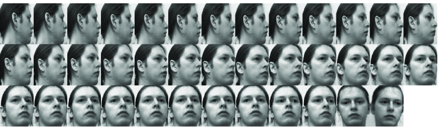
Figure 2: Sample UMIST face images.

We use the AR database [23] which contains 1,008 grayscale 768-by-576 images of 126 subjects, 8 images per subject. These images were cropped and downsized to be 224-by-184 before the recognition is performed in the experiments. Figure 3 presents the sample images of the first two subjects.

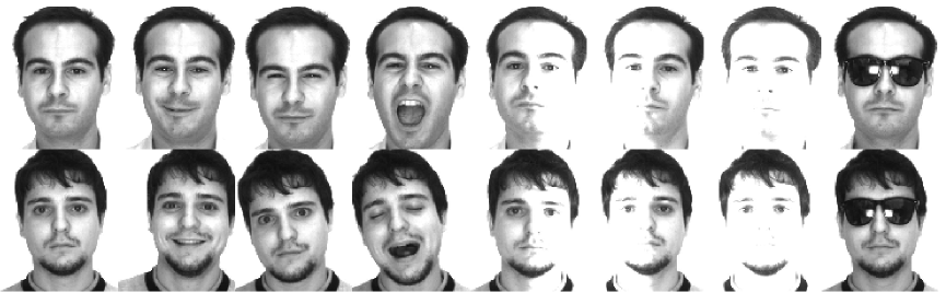
Figure 3: Sample AR face images.

We also use the ESSEX database [30]. The 95’ version contains 1,440 color 200-by-180 images of 72 subjects. Each subject has 20 images. We converted these color images to grayscale so they can be represented as matrices.

4.2 Performance sensitivity to repulsion

There are two parameters to select for the repulsion technique. One is the number $k$ of neighbors per vertex, used for constructing a repulsion graph. The other is the penalty parameter $\beta$, which determines the strength of the repulsion term.

To examine the sensitivity of the recognition performance to these parameters, we conducted two experiments as follows. We use the 2D-ONPP-R and 2D-OLPP-R methods, in both unilateral and bilateral projections. For unilateral projection, we set $d_{2}=10$ and the result is marked by ‘(U)’. For bilateral projection, we set $d_{1}=d_{2}=10$ and the result is marked by ‘(B)’. We use the images in the ORL database, and set the number of training images per class as 5. In one experiment, we set $k=6$ and $\beta=0.3,0.35,\dots,1$. In the other experiment, we set $k=1,2,\dots,20$ and $\beta=0.5$. The results are shown in Figure 4.

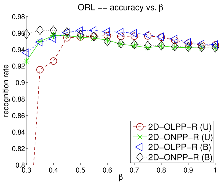
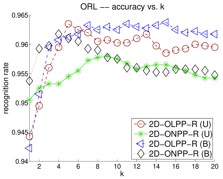
Figure 4: Sensitivity of performance to varying $\beta$ (left) and $k$ (right) for the ORL database.

It can be observed from Figure 4 that the recognition rate changes modestly as long as $\beta$ are $k$ are large enough.

4.3 Face recognition results

We report the results for 4 databases: ORL, UMIST, AR, and ESSEX. Regarding the repulsion parameters, we use $k=6$ in all cases. In both 2D-OLPP-R and 2D-ONPP-R, we set $\beta=0.5$, but for the ESSEX database, we set $\beta=1.0$. As discussed in Section 3.5, we need a smaller $\beta$ for 2D-LDA-R, in which we set $\beta=0.2$.

The results for the ORL database are displayed in Figure 5, where the number of training images per class is set as 5. The left plot shows the recognition rates with the unilateral projections with the column dimension $d_{2}=2,4,\dots,20$, whereas the right plot shows the recognition rates with the bilateral projections with the row/column dimension $d_{1}=d_{2}=2,4,\dots,20$.

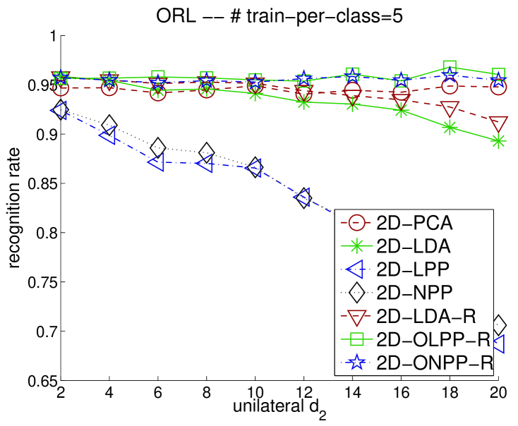
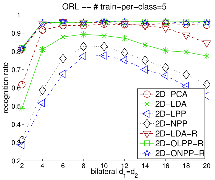
Figure 5: Accuracy versus dimension for the ORL database; unilateral projection (left) and bilateral projection (right).

Two observations from Figure 5 can be made.

1. In both settings of unilateral and bilateral projections, 2D-LDA-R improves 2D-LDA, and 2D-OLPP-R and 2D-ONPP-R outperform 2D-LPP and 2D-NPP handsomely.

2. 2D-OLPP-R is the best option for the ORL database, whereas 2D-ONPP-R is the close runner-up.

Table 3 lists the best recognition rates and the corresponding dimensions, using the 7 two-dimensional (2D) methods and their one-dimen-sional (1D) peers. On average, the 1D methods and 2D methods are comparable in performance. However, the 1D methods with repulsion Laplaceans perform slightly better than the 2D methods with repulsion tensors.

Table 3: Best achieved error rates and the corresponding dimensions for the ORL database.

1D Method			2D Method
method	# dim.	error	method	unilateral		bilateral
				# dim.	error	# dim.	error
PCA	90	5.12%	2D-PCA	10	5.10%	16	4.60%
LDA	65	6.95%	2D-LDA	2	4.15%	8	10.6%
LPP	60	10.8%	2D-LPP	2	7.60%	10	22.3%
NPP	15	9.50%	2D-NPP	2	7.53%	10	17.3%
LDA-R	70	2.90%	2D-LDA-R	2	4.23%	6	3.78%
OLPP-R	55	2.82%	2D-OLPP-R	18	3.20%	10	3.55%
ONPP-R	90	3.40%	2D-ONPP-R	18	4.03%	10	3.50%

Figure 6 displays the results for the UMIST database, where the number of training images is set as 10. Table 4 lists the best recognition rates and the corresponding dimensions. The observations made previously for the ORL image set are also valid here, except for that the performance of the 2D-LDA-R bilateral projection deteriorates quickly while the dimension increases. An explanation of this instability is given in Section 3.5. Among the two-dimensional methods, both 2D-OLPP-R and 2D-ONPP-R are the apparent winners for the UMIST and ORL databases.

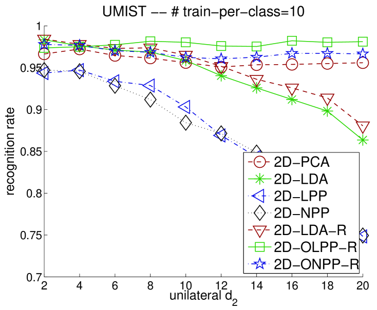
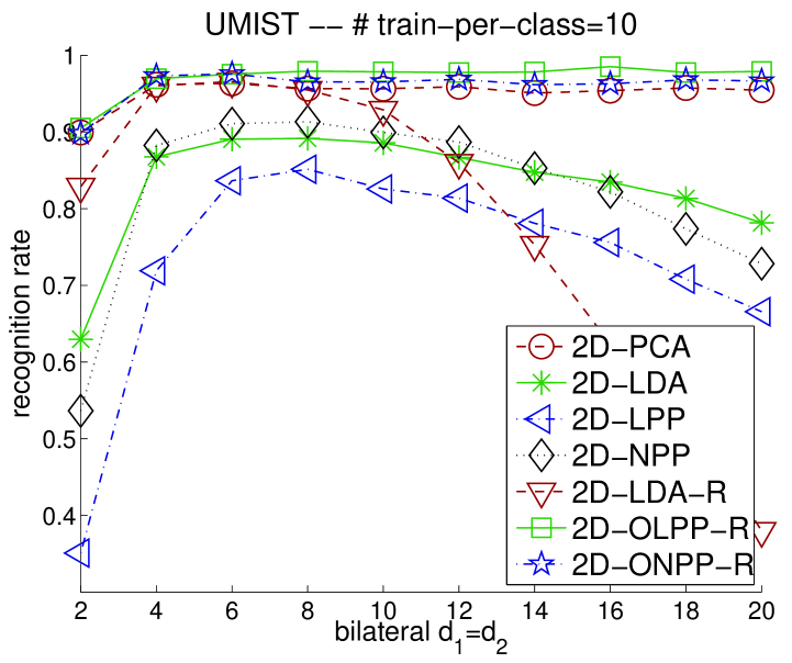
Figure 6: Accuracy versus dimension for the UMIST database; unilateral projection (left) and bilateral projection (right).

Table 4: Best achieved error rates and the corresponding dimensions for the UMIST database.

1D Method			2D Method
method	# dim.	error	method	unilateral		bilateral
				# dim.	error	# dim.	error
PCA	65	4.12%	2D-PCA	4	2.77%	6	3.67%
LDA	30	3.44%	2D-LDA	2	1.67%	8	1.07%
LPP	10	4.03%	2D-LPP	4	5.29%	8	1.48%
NPP	15	4.56%	2D-NPP	2	5.29%	8	8.66%
LDA-R	95	1.62%	2D-LDA-R	2	1.57%	6	3.44%
OLPP-R	30	0.93%	2D-OLPP-R	16	1.79%	16	1.48%
ONPP-R	15	1.45%	2D-ONPP-R	2	2.23%	6	2.42%

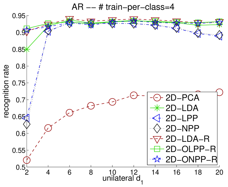
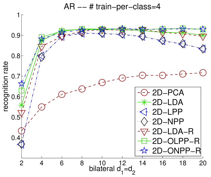
Figure 7: Accuracy versus dimension for the AR database; unilateral projection (left) and bilateral projection (right).

Table 5: Best achieved error rates and the corresponding dimensions for the AR database.

1D Method			2D Method
method	# dim.	error	method	unilateral		bilateral
				# dim.	error	# dim.	error
PCA	100	28.6%	2D-PCA	20	27.8%	20	28.3%
LDA	100	10.3%	2D-LDA	6	6.31%	8	7.03%
LPP	15	7.12%	2D-LPP	6	7.04%	8	9.10%
NPP	20	7.60%	2D-NPP	6	7.24%	8	8.66%
LDA-R	85	5.98%	2D-LDA-R	6	5.92%	14	7.25%
OLPP-R	75	3.96%	2D-OLPP-R	12	6.61%	18	6.66%
ONPP-R	45	4.04%	2D-ONPP-R	12	6.61%	12	6.76%

The results for the AR database are illustrated in Figure 7, where we set the number of training images as 4. Note that except for 2D-PCA, we pre-process the data by 2D-PCA, explained in Section 3.6. Table 5 lists the best recognition rates and the corresponding dimensions. 2D-ONPP-R and 2D-OLPP-R are still the best two-dimensional methods in performance. In addition, 2D-LDA-R with unilateral projection performs as good in this case. It is interesting to note that 2D-LPP and 2D-NPP yield very similar results. Also note that PCA and 2D-PCA does not perform that well for this case.

Figure 8 displays the results for the ESSEX database, where we set the number of training images as 10. Table 6 lists the best recognition rates and the corresponding dimensions. In this case, 2D-OLPP-R outperforms the other methods, including all 1D methods. This database is the hardest one tested in [16]. It hints the potential of the repulsion tensors for challenging classification tasks.

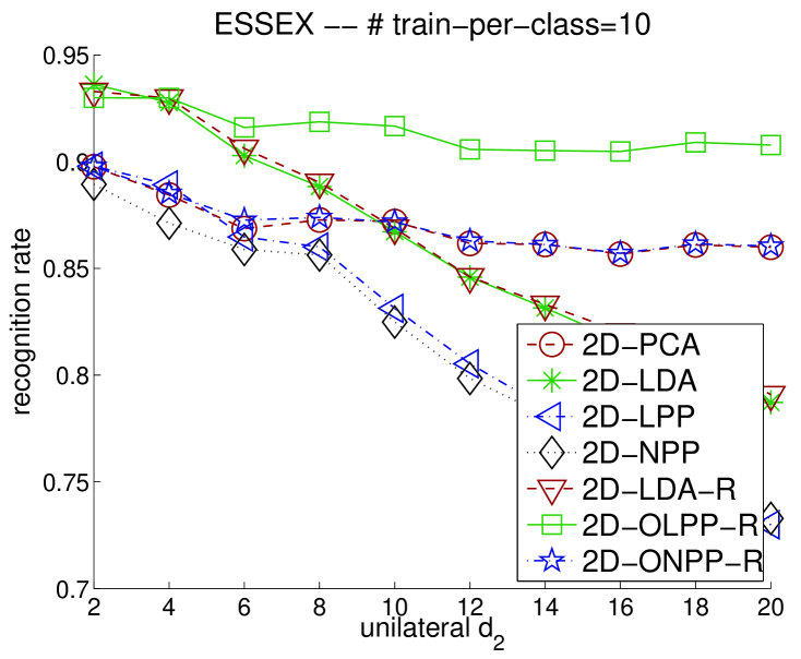
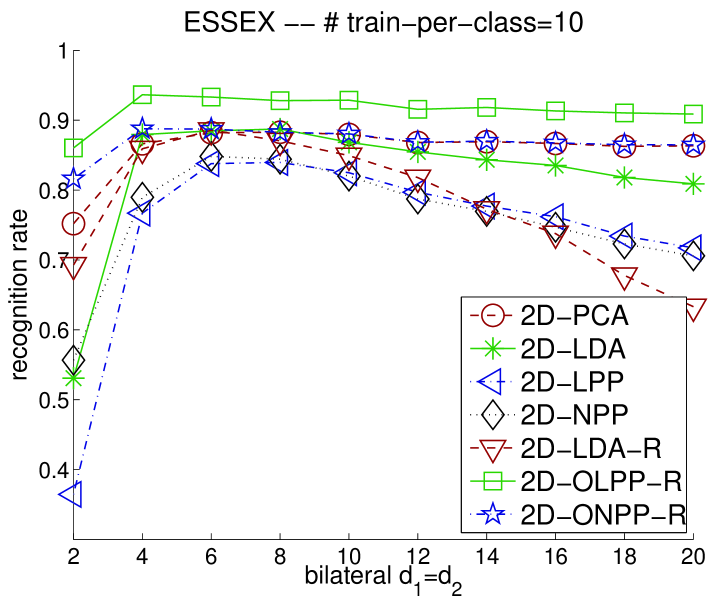
Figure 8: Accuracy versus dimension for the ESSEX database; unilateral projection (left) and bilateral projection (right).

Table 6: Best achieved error rates and the corresponding dimensions for the ESSEX database.

1D Method			2D Method
method	# dim.	error	method	unilateral		bilateral
				# dim.	error	# dim.	error
PCA	65	15.1%	2D-PCA	2	10.2%	8	11.7%
LDA	55	61.6%	2D-LDA	2	6.38%	8	11.3%
LPP	10	15.3%	2D-LPP	2	10.2%	8	16.0%
NPP	15	17.3%	2D-NPP	2	11.1%	6	15.2%
LDA-R	20	10.4%	2D-LDA-R	2	6.72%	6	11.4%
OLPP-R	25	12.5%	2D-OLPP-R	2	7.01%	4	6.35%
ONPP-R	65	9.88%	2D-ONPP-R	2	10.2%	4	11.2%

In addition to the attractive recognition rates by 2D-OLPP-R and 2D-ONPP-R. It is worth noting that the performance of 2D-OLPP-R and 2D-ONPP-R is very insensitive to the variation of the reduced dimension in all our tests. This is an appealing feature, especially considering that in real applications we may not have the labels of test images.

4.4 1D methods versus 2D methods

One-dimensional (1D) methods use the image-as-vector representation, whereas two-dimensional (2D) methods use the image-as-matrix representation. This fundamental difference governs the computation. Whether 2D methods or 1D methods are faster depends on several factors. For example, size of the images, number of training faces, how the algorithms are implemented, and the numerical libraries used, etc.

The high level idea is that 1D methods, which vectorize images, need to solve a much larger eigenvalue problem. On the other hand, the computation of the 2D methods is often dominated by forming the eigenvalue problem, i.e., computing (38), (39), (40), and (43). In practice, this part is usually less expensive than the eigenvalue computation of the 1D method. Indeed, it has been reported that 2D methods are more efficient than their 1D counterparts, e.g., [4, 25, 36, 37, 38]. We have also observed this property in our experiments. Note however that one can downsize the image matrices to reduce the cost of the eigenvalue computation.

5 Conclusions and future work

We have developed a methodology with repulsion tensors to enhance the two-dimensional projection methods for classification. It can be regarded as a multilinear generalization of a technique called repulsion Laplaceans [16]. The key idea is improve the projection by repelling data items which are from different classes but close to each other in the input space. The experiments on face recognition exhibit significant improvement of recognition performance by the proposed technique.

Some two-dimensional projection methods can be formulated as a tensor trace ratio optimization problem. Instead of solving this problem directly, we use Algorithm 2 as an efficient workaround. It may be worth developing efficient algorithms for the tensor trace ratio optimization problem.

All the methods presented in this paper are linear. Hence it may fail to discover the underlying latent structure if the image manifold is highly nonlinear. A research topic is how to learn the nonlinear structure of images or higher order tensor objects in the supervised setting.

Appendix A Basics of tensors

An $r$th order tensor is an array of $r$ indices. A vector is a first order tensor, and a matrix is a second order tensor. Different dimensions are also called modes. To facilitate the presentation, we will illustrate with third and fourth order tensors with specific modes. However, the definitions for higher order tensors in general modes can be straightforwardly extended. The readers are referred to [1] for details.

Let $\mathcal{A},\mathcal{B}\in\mathbb{R}^{I\times J\times K}$ be third order tensors, where $I,J,K$ are positive integers. The inner product $\langle\mathcal{A},\mathcal{B}\rangle$ of tensors $\mathcal{A},\mathcal{B}$ is defined by

$$\langle\mathcal{A},\mathcal{B}\rangle=\sum_{i=1}^{I}\sum_{j=1}^{J}\sum_{k=1}^{K}a_{ijk}b_{ijk}.$$ (46)

Two tensors $\mathcal{A},\mathcal{B}$ are orthogonal to each other if $\langle\mathcal{A},\mathcal{B}\rangle=0$. The Frobenius norm of a tenor $\mathcal{A}$ is defined by

$$\|\mathcal{A}\|=\sqrt{\langle\mathcal{A},\mathcal{A}\rangle}.$$ (47)

We can transform a higher order tensor to a matrix by merging dimensions and rearranging the elements. This is called ‘unfolding’ [18], ‘flattening’ [33], or ‘matricizing’ [1] a tensor.

For example, given a third order tensor $\mathcal{A}=[a_{ijk}]\in\mathbb{R}^{I\times J\times K}$, we can have

$$A_{(1)}=[a_{ip}^{(1)}]\in\mathbb{R}^{I\times JK}, a_{ijk}=a_{ip}^{(1)}, p=j+(k-1)J,$$

$$A_{(2)}=[a_{jp}^{(2)}]\in\mathbb{R}^{J\times IK}, a_{ijk}=a_{jp}^{(2)}, p=k+(i-1)K,$$

$$A_{(3)}=[a_{kp}^{(3)}]\in\mathbb{R}^{K\times IJ}, a_{ijk}=a_{kp}^{(3)}, p=i+(j-1)I,$$

where by default we have used the forward cyclic ordering. The other option of ordering is backward cyclic [1]. We use $A_{(1;2,3)}$ and $A_{(1;3,2)}$ to specify the forward and backward cyclic orderings, respectively. Here is another example to matricize a fourth order tensor $\mathcal{A}=[a_{ijkh}]\in\mathbb{R}^{I\times J\times K\times H}$ as

$$A_{(1,2;3,4)}=[a_{pq}^{(1,2;3,4)}],\;a_{ijkh}=a_{pq}^{(1,2;3,4)},$$ (48)

where $p=i+(j-1)I$ and $q=k+(h-1)K$.

The mode-$3$ product of a tensor $\mathcal{A}\in\mathbb{R}^{I\times J\times K}$ times a matrix $U\in\mathbb{R}^{H\times K}$ is defined by

$$(\mathcal{A}\times_{3}U)(i,j,h)=\sum_{k=1}^{K}a_{ijk}u_{hk}.$$

The tensor-matrix products in other modes are defined similarly.

The mode-$[3;3]$ contracted product of two third order tensors $\mathcal{A}\in\mathbb{R}^{I_{1}\times J_{1}\times K}$ and $\mathcal{B}\in\mathbb{R}^{I_{2}\times J_{2}\times K}$ is defined by

$$\langle\mathcal{A},\mathcal{B}\rangle_{[3;3]}(i_{1},j_{1},i_{2},j_{2})=\sum_{k=1}^{K}a_{i_{1}i_{2}k}b_{i_{2}j_{2}k},$$

where the first $3$ in $[3;3]$ indicates the third mode of $\mathcal{A}$, and the second $3$ refers to the third mode of $\mathcal{B}$. The definition can be generalized to different modes and multiple modes [1].

A useful property is that given $\mathcal{A}\in\mathbb{R}^{I\times J\times K}$, we let $\mathcal{B}=\langle\mathcal{A},\mathcal{A}\rangle_{[3;3]}$, and then have

$$\|\mathcal{A}\|^{2}=\mbox{tr}(B_{(1,2;3,4)}),$$ (49)

where $B_{(1,2;3,4)}$ is the result of matricization of $\mathcal{B}$. See (48) for the definition. With the tensor trace notation introduced in Section 2, we can write (49) as $\|\mathcal{A}\|^{2}=\mbox{tr}(\langle\mathcal{A},\mathcal{A}\rangle_{[3;3]}),$ which is the high order generalization of $\|A\|=\mbox{tr}(AA^{T}).$

Appendix B Image-as-vector methods

We review the linear dimensionality reduction methods which transform $X=[x_{1},x_{2},\dots,x_{n}]\in\mathbb{R}^{m\times n}$ into $Y=[y_{1},y_{2},\dots,y_{n}]\in\mathbb{R}^{d\times n}$ ($d<m$) by a linear mapping $Y=U^{T}X$ in order to preserve some properties. This matrix $U$ can be applied to project test data for recognition tasks. If the original numerical data items, such as face images, are not one-dimensional, they are converted to column vectors $x_{1},x_{2},\dots,x_{n}\in\mathbb{R}^{m}$. The mapping is called orthogonal, if $U\in\mathbb{R}^{m\times d}$ consists of orthonormal columns, i.e., $U^{T}U=I_{d}$.

B.1 Principal component analysis

Principal Component Analysis (PCA) performs an orthogonal mapping $Y=U^{T}X$ to maximize the variance of the projected vectors. More precisely, the objective function to maximize is

$$\sum_{i=1}^{n}\|y_{i}-\bar{y}\|^{2}=\|Y-\bar{y}e_{n}^{T}\|^{2}=\|Y-(\frac{1}{n}Ye_{n})e_{n}^{T}\|^{2}=\|U^{T}X(I_{n}-\frac{1}{n}e_{n}e_{n}^{T})\|^{2}$$ (50)

subject to $U^{T}U=I_{d}$, where $\bar{y}=\frac{1}{n}\sum_{j=1}^{n}y_{j}$ is the mean and $e_{n}\in\mathbb{R}^{n}$ is the column vector of ones. Hence the maximizer of (50) is the left $d$ singular vectors of $X(I_{n}-\frac{1}{n}e_{n}e_{n}^{T})$ corresponding to the largest $d$ singular values, or equivalently the top $d$ eigenvectors of $X(I_{n}-\frac{1}{n}e_{n}e_{n}^{T})X^{T}$. Note that $J_{n}:=I_{n}-\frac{1}{n}e_{n}e_{n}^{T}$ is a projection matrix and therefore $J_{n}^{2}=J_{n}=J_{n}^{T}$.

In the methods described subsequently in this appendix, it is common to pre-process the training data matrix $X$ by PCA, in order to avoid a singular matrix in the eigenvalue computation. By abuse of notation, we also denote by $X$ the resulting matrix preprocessed by PCA.

B.2 Affinity graph

Several dimensionality reduction methods utilize an affinity graph $G=(V,E)$, where $V=\{1,\dots,n\}$ consists of indices of data items. Data item $j$ is deemed related to data item $i$ if $(i,j)\in E$. If the input data are unsupervised, one may construct a $k\mbox{NN}$ graph or an $\epsilon$-graph for an affinity graph. The graph is made undirected if symmetry is desired. In supervised learning, each data item is associated with a class label. For example, in face recognition, each training image is of subject. A label graph $G=(V,E)$ is defined by that $(i,j)\in E$ if data items $i$ and $j$ have the same label, i.e., in the same class. It has been observed that supervised graphs often outperform their unsupervised peers in the recognition tasks.

Each edge $(i,j)\in E$ is associated with a weight $w_{ij}$ as the measure of influence between the two neighboring points $i$ and $j$. A popular choice is the Gaussian weights:

$$w_{ij}=\left\{\begin{array}[]{ll}e^{-\|x_{i}-x_{j}\|^{2}/t}&\mbox{if }(i,j)\in E,\\ 0&\mbox{otherwise},\end{array}\right.$$ (51)

where $t>0$ is some constant. Alternatively, we can use the binary weights from driving $t\rightarrow 0$. It is common to employ an undirected affinity graph when the Gaussian weights or the induced binary weights are used.

Another weighting scheme, proposed in the Locally Linear Embedding (LLE) [27], is from minimizing the function

$$\left\{\begin{array}[]{ll}\displaystyle\mathop{\mbox{minimize}}_{w_{ij}}&\displaystyle\sum_{i=1}^{n}\|x_{i}-\sum_{j=1}^{n}w_{ij}x_{j}\|^{2}\\ \textup{subject to}&w_{ij}=0\mbox{ for }(i,j)\notin E,\\ &\sum_{j=1}^{n}w_{ij}=1\mbox{ for all }i.\end{array}\right.$$ (52)

subject to $w_{ij}=0$ if $(i,j)\notin E$, and $\sum_{j=1}^{n}w_{ij}=1$ for $i=1,\dots,n$. The minimizer of (52) is obtained from solving $n$ symmetric linear systems. See [27] for more information. Note that the resulting weights are usually asymmetric and can be negative. The discussion on the affinity graph and the weighting scheme applies not only to this appendix but also to Sections 2 and 3.

B.3 Locality preserving projection

Consider the objective function to minimize: $\frac{1}{2}\sum_{i,j=1}^{n}w_{ij}\|y_{i}-y_{j}\|^{2},$ where $w_{ij}$’s are non-negative weights, e.g., the Gaussian weights (51). In what follows we need the weight matrix $W=[w_{ij}]\in R^{n\times n}$ being symmetric. Let $D\in\mathbb{R}^{n\times n}$ be the diagonal matrix formed by $d_{ii}=\sum_{j=1}^{n}w_{ij}$, and denote the graph Laplacian by $L=D-W$. After some algebra, we have

$$\frac{1}{2}\sum_{i,j=1}^{n}w_{ij}\|y_{i}-y_{j}\|^{2}=\mbox{tr}(YLY^{T}).$$ (53)

Laplacian eigenmaps [2] is a nonlinear dimensionality reduction method that minimizes (53) subject to $YDY^{T}=I_{d}$ and $YDe_{n}=0$. Locality Preserving Projection (LPP) [9, 10] also minimizes (53), but imposes the linear projection constraint $Y=U^{T}X$ and solves

$$\left\{\begin{array}[]{ll}\displaystyle\mathop{\mbox{minimize}}_{U}&\displaystyle\mbox{tr}(U^{T}XLX^{T}U)\\ \textup{subject to}&U^{T}XDX^{T}U=I_{d}.\end{array}\right.$$ (54)

This is equivalent to solving the generalized eigenvalue problem

$$XLX^{T}u_{i}=\lambda_{i}XDX^{T}u_{i}.$$ (55)

The minimizer of the program (54) is

$$U=[u_{1},\dots,u_{d}]\in\mathbb{R}^{n\times d},$$

where $u_{1},\dots,u_{d}$ are the eigenvectors corresponding to the smallest generalized eigenvalues of (55). Note that the program (54) can be regarded as a workaround to minimize $\mbox{tr}(U^{T}XLX^{T}U)$ and maximize $\mbox{tr}(U^{T}XDX^{T}U)$ concurrently.

Another option is to replace the constraint $U^{T}XDX^{T}U=I_{d}$ in (54) by simply the orthogonal mapping, i.e., $U^{T}U=I_{d}$, and then the minimizer $U$ of (53) consists of the $d$ eigenvectors of $XLX^{T}$, corresponding to the $d$ smallest eigenvalues. We call this method the Orthogonal Locality Preserving Projection (OLPP) [15, 16]. In practice, we use the supervised label graph and the Gaussian weights (51) for both LPP and OLPP.

B.4 Neighborhood preserving projection

The nonlinear dimensionality reduction method LLE [27] minimizes

$$\sum_{i=1}^{n}\|y_{i}-\sum_{j=1}^{n}w_{ij}y_{j}\|^{2}=\|Y-YW^{T}\|^{2}$$ (56)

subject to $YY^{T}=I_{d}$ and $Ye_{n}=0$.

One can impose the linear projection $Y=U^{T}X$ and solve

$$\left\{\begin{array}[]{ll}\displaystyle\mathop{\mbox{minimize}}_{U}&\displaystyle\|U^{T}X(I_{n}-W)^{T}\|^{2}\\ \textup{subject to}&U^{T}XX^{T}U=I_{d}.\end{array}\right.$$ (57)

We call the resulting method Neighborhood Preserving Projection (NPP) [8]. The minimizer of (57) consists of the $d$ eigenvectors corresponding to the $d$ smallest generalized eigenvalues of

$$X(I_{n}-W)^{T}(I_{n}-W)X^{T}u_{i}=\lambda_{i}XX^{T}u_{i}.$$

A related method, Orthogonal Neighborhood Preserving Projections (ONPP) [14, 15], solves

$$\left\{\begin{array}[]{ll}\displaystyle\mathop{\mbox{minimize}}_{U}&\displaystyle\|U^{T}X(I_{n}-W)^{T}\|^{2}\\ \textup{subject to}&U^{T}U=I_{d},\end{array}\right.$$ (58)

which replaces $U^{T}XX^{T}U=I_{d}$ in (57) by the $U^{T}U=I_{d}$. The solution is formed by the $d$ left singular vectors of $X(I_{n}-W)^{T}$ corresponding to the $d$ smallest singular values, or equivalently the bottom $d$ eigenvectors of $X(I_{n}-W)^{T}(I_{n}-W)X^{T}$. Note that both NPP and ONPP do not need weights being symmetric. Therefore, it is common to adopt the weighting scheme (52) of LLE.

It is interesting to note that $(I_{n}-W)^{T}(I_{n}-W)$ in NPP and ONPP plays the role of the Laplacian matrix $L$ in LPP and OLPP [13]. This observation is important to the repulsion techniques in [16] and in this paper.

B.5 Linear discriminant analysis

The method of Linear Discriminant Analysis (LDA) [3, 5] can be formulated as follows. Suppose we are given high dimensional data $X=[x_{1},x_{2},\dots,x_{n}]\in\mathbb{R}^{m\times n}$ with each data sample $x_{i}$ associated with a class label $c(i)$. Let

$$\mathcal{C}_{j}=\{i:c(i)=j\}$$

be the index set of all data items in class $j$, and $n_{j}=|\mathcal{C}_{j}|$ be the size of class $j$. The mean of each class $j$ is denoted by $\bar{x}_{j}=\frac{1}{n_{j}}\sum_{i\in\mathcal{C}_{j}}x_{i}$, and the global mean is $\bar{x}=\frac{1}{n}\sum_{i=1}^{n}x_{i}$. The within-scatter matrix of $X$ is defined by

$$S_{w}=\sum_{j}\sum_{i\in\mathcal{C}_{j}}(x_{i}-\bar{x}_{j})(x_{i}-\bar{x}_{j})^{T},$$ (59)

and the between-scatter matrix of $X$ is

$$S_{b}=\sum_{j}n_{j}(\bar{x}-\bar{x}_{j})(\bar{x}-\bar{x}_{j})^{T}.$$ (60)

Since the lower dimensional data are obtained by a linear mapping $Y=U^{T}X\in\mathbb{R}^{d\times n}$, the between-scatter matrix and within-scatter matrix of $Y$ are $U^{T}S_{w}U$ and $U^{T}S_{b}U$, respectively.

We would like to maximize $\mbox{tr}(U^{T}S_{b}U)$ and minimize $\mbox{tr}(U^{T}S_{w}U)$ in some way. It is common to solve

$$\left\{\begin{array}[]{ll}\displaystyle\mathop{\mbox{maximize}}_{U}&\displaystyle\mbox{tr}(U^{T}S_{b}U)\\ \textup{subject to}&U^{T}S_{w}U=I_{d},\end{array}\right.$$ (61)

The maximizer of (61) is $U=[u_{1},\dots,u_{d}]$, the $d$ largest generalized eigenvalues of

$$S_{b}u_{i}=\lambda_{i}S_{w}u_{i}.$$

Note that LPP can be regarded a generalization of LDA. See [10] for a discussion.

In comparison, the projections of LPP, OLPP, NPP, and ONPP can be performed in either supervised or unsupervised mode, whereas the PCA projection is unsupervised and the LDA projection is supervised.

References

- [1] B. W. Bader and T. G. Kolda. Algorithm 862: MATLAB tensor classes for fast algorithm prototyping. ACM Transactions on Mathematical Software, 32(4):635–653, December 2006.
- [2] M. Belkin and P. Niyogi. Laplacian eigenmaps for dimensionality reduction and data representation. Neural Comput., 15(6):1373–1396, 2003.
- [3] P. N. Bellhumeur, J. P. Hespanha, and D. J. Kriegman. Eigenfaces vs. Fisherfaces: Recognition using class specific linear projection. IEEE Trans. Pattern Anal. and Mach. Intell., 19(7):711–720, 1997.
- [4] S. Chen, H. Zhao, M. Kong, and B. Luo. 2d-lpp: A two-dimensional extension of locality preserving projections. Neurocomput., 70, 2007.
- [5] R. A. Fisher. The use of multiple measurements in taxonomic problems. Annals of Eugenics, 7(2):179–188, 1936.
- [6] D. B. Graham and N. M. Allinson. Face recognition: From theory to applications. In H. Wechsler, P. J. Phillips, V. Bruce, F. Fogelman-Soulie, and T. S. Huang, editors, NATO ASI Series F, Computer and Systems Sciences, Vol. 163, pages 446–456, 1998.
- [7] X. He, D. Cai, and P. Niyogi. Tensor subspace analysis. In Advances in Neural Information Processing Systems 18 (NIPS), 2005.
- [8] X. He, D. Cai, S. Yan, and H.-J. Zhang. Neighborhood preserving embedding. In IEEE International Conference on Computer Vision (ICCV), pages 1208–1213, 2005.
- [9] X. He and P. Niyogi. Locality preserving projections. In Advances in Neural Information Processing Systems 16 (NIPS), 2003.
- [10] X. He, S. Yan, Y. Hu, P. Niyogi, and H.-J. Zhang. Face recognition using Laplacianfaces. IEEE Trans. Pattern Anal. and Mach. Intell., 27(3):328–340, 2005.
- [11] X.-Y. Jing, H.-S. Wong, and D. Zhang. Face recognition based on 2D Fisherface approach. Pattern Recognition, 39(4):707–710, 2006.
- [12] I.T. Jolliffe. Principal Component Analysis. Springer, 2nd edition, 2002.
- [13] E. Kokiopoulou, J. Chen, and Y. Saad. Trace optimization and eigenproblems in dimension reduction methods. Numer. Linear Algebra Appl., 18(3):565–602, 2011.
- [14] E. Kokiopoulou and Y. Saad. Orthogonal neighborhood preserving projections. In The 5th IEEE International Conference on Data Mining (ICDM), pages 234–241, 2005.
- [15] E. Kokiopoulou and Y. Saad. Orthogonal neighborhood preserving projections: A projection-based dimensionality reduction technique. IEEE Trans. Pattern Anal. and Mach. Intell., 29(12):2143–2156, 2007.
- [16] E. Kokiopoulou and Y. Saad. Enhanced graph-based dimensionality reduction with repulsion Laplaceans. Pattern Recognition, 42(11):2392–2402, 2009.
- [17] H. Kong, L. Wang, E. K. Teoh, X. Li, J.-G. Wang, and R. Venkateswarlu. Generalized 2D principal component analysis for face image representation and recognition. Neural Networks, 18(5-6):585–594, 2005.
- [18] L. D. Lathauwer, B. D. Moor, and J. Vandewalle. A multilinear singular value decomposition. SIAM J. Matrix Anal. Appl., 21(4):1253–1278, 2000.
- [19] L. D. Lathauwer, B. D. Moor, and J. Vandewalle. On the best rank- and rank- approximation of higher-order tensors. SIAM J. Matrix Anal. Appl., 21(4):1324–1342, 2000.
- [20] M. Li and B. Yuan. A novel statistical linear discriminant analysis for image matrix: Two-dimensional Fisherfaces. In The 8th International Conference on Signal Processing (ICSP), pages 1419–1422, 2004.
- [21] M. Li and B. Yuan. 2D-LDA: A statistical linear discriminant analysis for image matrix. Pattern Recogn. Lett., 26(5):527–532, 2005.
- [22] Z. Li and M. Du. 2d-npp: An extension of neighborhood preserving projection. In IEEE International Conference on Computational Intelligence and Security, pages 410–414, 2007.
- [23] A. M. Martínez and A. C. Kak. PCA versus LDA. IEEE Trans. Pattern Anal. and Mach. Intell., 23(2):228–233, 2001.
- [24] T. T. Ngo, M. Bellalij, and Y. Saad. The trace ratio optimization problem for dimensionality reduction. SIAM J. Matrix Anal. Appl., 31(5):2950–2971, 2010.
- [25] B. Niu, Q. Yang, S. C. K. Shiu, and S. K. Pal. Two-dimensional Laplacianfaces method for face recognition. Pattern Recognition, 41:3237–3242, 2008.
- [26] C.-X. Ren and D.-Q. Dai. 2d-onpp: Two dimensional extension of orthogonal neighborhood preserving projections for face recognition. In Chinese Conference on Pattern Recognition (CCPR), pages 1–6, 2008.
- [27] S. T. Rowies and L. K. Saul. Nonlinear dimensionality reduction by locally linear embedding. Science, 290:2323–2326, 2000.
- [28] F. S. Samaria and A. C. Harter. Parameterisation of a stochastic model for human face identification. In Proceedings of 2nd IEEE Workshop on Applications of Computer Vision, pages 138–142, 1994.
- [29] B. N. Sheeban and Y. Saad. Higher order orthogonal iteration of tensors (HOOI) and its relation to PCA and GLRAM. In SIAM International Conference on Data Mining (SDM), pages 355–365, 2007.
- [30] L. Spacek. University of ESSEX face database, 2002. http://cswww.essex.ac.uk/mv/allfaces/index.html.
- [31] M. Turk and A. Pentland. Eigenfaces for recognition. Journal of Cognitive Neuroscience, 3(1):71–86, 1991.
- [32] M. Turk and A. Pentland. Face recognition using eigenfaces. In IEEE Computer Society Conference on Computer Vision and Pattern Recognition (CVPR), pages 586–591, 1991.
- [33] M. A. O. Vasilescu and D. Terzopoulos. Multilinear subspace analysis of image ensembles. In Proc. of the European Conf. on Computer Vision (ECCV), pages 447–460, 2002.
- [34] H. Wang, S. Yan, D. Xu, X. Tang, and T. S. Huang. Trace ratio vs. ratio trace for dimensionality reduction. In IEEE Computer Society Conference on Computer Vision and Pattern Recognition CVPR, 2007.
- [35] D. Xu, S. Yan, L. Zhang, S. Lin, H.-J. Zhang, and T. S. Huang. Reconstruction and recognition of tensor-based objects with concurrent subspaces analysis. IEEE Trans. Circuits and Systems for Video Technology, 18(1):36–47, Jan. 2008.
- [36] J. Yang, D. Zhang, A. F. Frangi, and J.-y. Yang. Two-dimensional PCA: A new approach to appearance-based face representation and recognition. IEEE Trans. Pattern. Anal. Mach. Intell., 26(1):131–137, 2004.
- [37] J. Ye. Generalized low rank approximations of matrices. J. of Machine Learning, 61:167–191, 2005.
- [38] J. Ye, R. Janardan, and Q. Li. Two-dimensional linear discriminant analysis. In Advances in Neural Information Processing Systems 17 (NIPS), 2004.