A preconditioner for the Ohta–Kawasaki equation

Abstract

We propose a new preconditioner for the Ohta–Kawasaki equation, a nonlocal Cahn–Hilliard equation that describes the evolution of diblock copolymer melts. We devise a computable approximation to the inverse of the Schur complement of the coupled second-order formulation via a matching strategy. The preconditioner achieves mesh independence: as the mesh is refined, the number of Krylov iterations required for its solution remains approximately constant. In addition, the preconditioner is robust with respect to the interfacial thickness parameter if a timestep criterion is satisfied. This enables the highly resolved finite element simulation of three-dimensional diblock copolymer melts with over one billion degrees of freedom.

1 Introduction

The Ohta–Kawasaki equations [11] model the evolution of diblock copolymer melts. A diblock copolymer is a polymer consisting of two subchains of different monomers that repel each other but are joined by a covalent bond. A large collection of these molecules is termed a melt. These melts are of scientific and engineering interest because they undergo phase separation of their different constituent monomers, allowing for the design of nanostructures with particular desirable properties. The numerical simulation of these equations is an essential tool in exploring the associated phase diagram [3].

The Ohta–Kawasaki functional describes the free energy of a diblock copolymer melt:

$$E[u]=\frac{1}{2}\int_{\Omega}\left(\varepsilon^{2}\left|\nabla u\right|^{2}\vphantom{\left|(-\Delta_{N})^{-1/2}(u-m)\right|^{2}}\right.+\frac{1}{2}\left(1-u^{2}\right)^{2}+\left.\sigma\left|(-\Delta_{N})^{-1/2}(u-m)\right|^{2}\right)\ \mathrm{d}x,$$ (1)

where $u=\pm 1$ denotes the two pure phases, $\Omega$ is the domain under study ($(0,1)^{2}$ or $(0,1)^{3}$), $\varepsilon\ll 1$ is the interfacial thickness between regions of the pure phases, $\sigma$ is the nonlocal energy coefficient, $m$ is the (conserved) average value of $u$ in $\Omega$, and $\Delta_{N}$ denotes the Laplacian with homogeneous Neumann boundary conditions. Assuming that the dynamics are governed by a $H^{-1}(\Omega)$ gradient flow,

$$(u_{t},\phi)_{H^{-1}(\Omega)}+E^{\prime}[u;\phi]=0,$$ (2)

the resulting Ohta–Kawasaki dynamic equation on $\Omega\times(0,T]$ in second-order form is given by [12]

$$u_{t}-\Delta w+\sigma(u-m) =0,$$ (3a)

$$w+\varepsilon^{2}\Delta u-u(u^{2}-1) =0,$$ (3b)

with homogeneous Neumann boundary conditions

$$\nabla u\cdot n=0\text{ and }\nabla w\cdot n=0,$$ (4)

and with initial condition $u(x,0)=u_{0}(x)$.

2 Approximating the Schur complement

After applying a finite element discretization in space and the $\theta$-method in time, a discrete nonlinear problem must be solved at each timestep. Each Newton iteration involves solving a linear system of the form

$$J\begin{bmatrix}\delta u\\ \delta w\\ \end{bmatrix}=\begin{bmatrix}(1+\Delta t\theta\sigma)M&\Delta t\theta K\\ -\varepsilon^{2}K-M_{E}&M\end{bmatrix}\begin{bmatrix}\delta u\\ \delta w\\ \end{bmatrix}=\begin{bmatrix}f_{1}\\ f_{2}\\ \end{bmatrix}.$$ (5)

where $J$ is the Jacobian, $M$ is the standard mass matrix with entries of the form $\int_{\Omega}\phi_{i}\phi_{j}\ \mathrm{d}x$, $K$ is the standard discretization of the Neumann Laplacian with entries $\int_{\Omega}\nabla\phi_{i}\cdot\nabla\phi_{j}\ \mathrm{d}x$, $M_{E}$ is a mass matrix involving a spatially varying coefficient with entries $\int_{\Omega}(3u^{2}-1)\phi_{i}\phi_{j}\ \mathrm{d}x$, $\delta u$ is the update for $u$, $\delta w$ is the update for $w$, $f_{1}$ and $f_{2}$ gather the source term and contributions from previous time levels, and $\Delta t$ is the timestep. As the discretization is refined and the dimension of (5) increases, it becomes impractical to employ direct solvers and preconditioned Krylov methods must be used instead. As the matrix in (5) is nonsymmetric, a suitable iterative solver such as GMRES [14] is required to compute its solution.

We note however that there are structures within the system that can be exploited within a solver. For example, $M$ is symmetric positive definite, $K$ is symmetric positive semidefinite (with one zero eigenvalue corresponding to the nullspace of constants), and $M_{E}$ is symmetric.

Preconditioners for block-structured matrices typically involve approximating the Schur complement of the system. Let the Jacobian $J$ be partitioned as

$$J=\begin{bmatrix}A&B\\ C&D\end{bmatrix}.$$ (6)

Consider the preconditioner

$$P^{-1}=\begin{bmatrix}A&0\\ C&S\end{bmatrix}^{-1}=\begin{bmatrix}A^{-1}&0\\ 0&S^{-1}\end{bmatrix}\begin{bmatrix}I&0\\ -CA^{-1}&I\end{bmatrix},$$ (7)

where $S=D-CA^{-1}B$ is the Schur complement with respect to $A$. If exact inner solves are used for $A^{-1}$ and $S^{-1}$, then the preconditioned operator $P^{-1}J$ has minimal polynomial degree two and GMRES converges exactly in two iterations [8, 10]. Here, $A$ is a scaled mass matrix and is thus straightforward to solve with standard techniques such as Chebyshev semi-iteration. Thus, the efficient preconditioning of $S$ is the key to the fast solution of the Newton step (5), and thus of the dynamic Ohta–Kawasaki equations (3a)–(3b).

The Schur complement of (5) is

$$S=M+\varepsilon^{2}cKM^{-1}K+cM_{E}M^{-1}K,$$ (8)

with constant $c={(\Delta t\theta)}/{(1+\Delta t\theta\sigma)}>0$. In general it is very difficult to precondition the sum of different matrices. The approach adopted here is the matching strategy of Pearson and Wathen [13, 2]: the sum is approximated by the product of matrices, carefully chosen to match as many terms of the sum as possible. We propose the approximation

$$S\approx\tilde{S}=\hat{S}M^{-1}\hat{S},$$ (9)

with

$$\hat{S}=M+\varepsilon\sqrt{c}K.$$ (10)

This approximation $\tilde{S}$ is the product of three invertible matrices, and so its inverse action can be efficiently computed by

$$\tilde{S}^{-1}=\hat{S}^{-1}M\hat{S}^{-1}.$$ (11)

The action of $\hat{S}^{-1}$ can be efficiently approximated with algebraic multigrid techniques [7] to yield a computationally cheap preconditioner.

Expanding the approximation (9), we find that it matches the first two terms of the Schur complement exactly:

$$\tilde{S}=M+\varepsilon^{2}cKM^{-1}K+2\varepsilon\sqrt{c}K.$$ (12)

Recall that $M_{E}$ depends on the current estimate of the solution $u$. With this matching strategy, the term involving $M_{E}$ in the Schur complement (8) has been neglected, so that $\tilde{S}$ does not vary between Newton iterations and no reassembly or algebraic multigrid reconstruction is required. The Schur complement approximation $\tilde{S}$ is straightforward and feasible to apply, and its effectiveness within a preconditioner will depend to a large extent on the effect of the neglected third term from $S$. In the next section we present some analysis to explain why we expect our approximation to work well as a preconditioner.

We note in passing that it is possible to rearrange (5) to the symmetric form

$$\begin{bmatrix}\frac{\Delta t\theta}{1+\Delta t\theta\sigma}K&M\\ M&-\varepsilon^{2}K-M_{E}\end{bmatrix}\begin{bmatrix}\delta w\\ \delta u\\ \end{bmatrix}=\begin{bmatrix}\frac{1}{1+\Delta t\theta\sigma}f_{1}\\ f_{2}\\ \end{bmatrix}.$$

It is likely that a similar approach could be used to precondition this rearranged system, providing one takes into account the singular $(1,1)$-block. Furthermore, as discussed in the next section, it is more straightforward to prove the rates of convergence of iterative methods for symmetric systems. However, whereas the $(1,1)$-block $A$ of (5) may be well approximated using Chebyshev semi-iteration, the stiffness matrix $K$ arising in the $(1,1)$-block of the rearranged system would require a more expensive method such as a multigrid process. We therefore prefer to solve the nonsymmetric system (5) due to the ease with which we may compute the approximate action of $A^{-1}$.

3 Analysis

We now wish to justify why our preconditioner is likely to be effective for the problem being solved. It is well-known that for nonsymmetric matrix systems it is extremely difficult to provide a concrete proof for the rate of convergence of an iterative method, as opposed to symmetric systems for which convergence is controlled only by the eigenvalues of the preconditioned system $P^{-1}J$. For nonsymmetric operators the spectrum alone does not determine the convergence of GMRES [6]; furthermore, the usual techniques for establishing eigenvalue bounds do not apply to the nonsymmetric case [2]. However, in practice, the tight clustering of eigenvalues for the preconditioned system frequently leads to strong convergence properties, even though this is not theoretically guaranteed. Given the challenges faced when solving nonsymmetric matrix systems, we present an analysis that establishes spectral equivalence of a slightly perturbed operator, and corroborate this analysis with numerical experiments in section 4 which demonstrate mesh independence for the full problem.

Observe that when applying the preconditioner

$$\ \begin{bmatrix}\tilde{A}&0\\ C&\tilde{S}\end{bmatrix}^{-1}=\begin{bmatrix}\tilde{A}^{-1}&0\\ 0&\tilde{S}^{-1}\end{bmatrix}\begin{bmatrix}I&0\\ -C\tilde{A}^{-1}&I\end{bmatrix}$$ (13)

for the Jacobian $J$, the crucial steps are applying $\tilde{A}^{-1}$ and $\tilde{S}^{-1}$. For the matrix system (5), the inverse of the sub-block $A=(1+\Delta{}t\theta\sigma)M$ may be approximated accurately and cheaply using a Jacobi iteration or Chebyshev semi-iteration [4, 5, 15]. It is therefore instructive to consider the preconditioned system

$$\ \begin{bmatrix}A&0\\ C&\tilde{S}\end{bmatrix}^{-1}\begin{bmatrix}A&B\\ C&D\end{bmatrix}=\begin{bmatrix}A^{-1}&0\\ 0&\tilde{S}^{-1}\end{bmatrix}\begin{bmatrix}I&0\\ -CA^{-1}&I\end{bmatrix}\begin{bmatrix}A&B\\ C&D\end{bmatrix}=\begin{bmatrix}I&A^{-1}B\\ 0&\tilde{S}^{-1}S\end{bmatrix},$$ (14)

where the inexactness of our preconditioner arises from the stated approximation $\tilde{S}$ of the Schur complement $S$. The eigenvalues of this system, which serve as a guide as to the effectiveness of the preconditioner, are either equal to $1$, or correspond to the eigenvalues of $\tilde{S}^{-1}S$.

We therefore examine the spectrum of the preconditioned Schur complement $\tilde{S}^{-1}S$, the matrix which governs the effectiveness of our algorithm, in the ideal setting where the matrix $M+\varepsilon\sqrt{c}K$ is inverted exactly. We first present a short result concerning the reality of the eigenvalues.

Lemma 1.

The eigenvalues of $\tilde{S}^{-1}S$ are real.

Proof.

If $v\in\textrm{null}(K)$ and $v\neq 0$, then

$$Sv=\lambda\tilde{S}v$$ (15)

implies

$$Mv=\lambda Mv,$$ (16)

and hence $\lambda=1\in\mathbb{R}$.

On the other hand, if $v\notin\textrm{null}(K)$, then (15) implies

$$\ KM^{-1}Sv=\lambda{}KM^{-1}\tilde{S}v~{}~{}\Rightarrow~{}~{}Fv=\lambda Gv~{}~{}\Rightarrow~{}~{}v^{*}Fv=\lambda v^{*}Gv,$$ (17)

where the matrices $F$ and $G$ are given by

$$F =K+\varepsilon^{2}cKM^{-1}KM^{-1}K+cKM^{-1}M_{F}M^{-1}K,$$ (18)

$$G =K+\varepsilon^{2}cKM^{-1}KM^{-1}K+2\varepsilon\sqrt{c}KM^{-1}K.$$ (19)

Using the symmetry of $F$ and $G$, it follows that $v^{*}Fv$ and $v^{*}Gv$ are real and positive, and hence $\lambda\in\mathbb{R}$. ∎

To motivate why $\tilde{S}$ should serve as an effective approximation of $S$, we now present a result on the eigenvalues of $\tilde{S}^{-1}S$ in the perturbed setting that $K$ is symmetric positive definite. (The matrix $K$ is in practice positive semidefinite, with a nullspace of dimension one.)

Lemma 2.

Perturb $K$ to be symmetric positive definite. Then the eigenvalues of $\tilde{S}^{-1}S$ satisfy:

$$\ \lambda(\tilde{S}^{-1}S)\in\left[\frac{1}{2}+\frac{1}{2\varepsilon}\hskip 1.00006pt\sqrt{c}\hskip 1.00006pt\lambda_{-},1+\frac{1}{2\varepsilon}\hskip 1.00006pt\sqrt{c}\hskip 1.00006pt\lambda_{+}\right),$$ (20)

where $\lambda_{-}=\min\{\lambda_{\min}(M^{-1}M_{E}),0\}$, $\lambda_{+}=\max\{\lambda_{\max}(M^{-1}M_{E}),0\}$ respectively, and $\lambda_{\min}$, $\lambda_{\max}$ are the minimum and maximum eigenvalues of a matrix.

Proof.

First note that the eigenvalues of $\tilde{S}^{-1}S$ and $S\tilde{S}^{-1}$ are the same by the similarity of the two matrices. We therefore examine the matrix $S\tilde{S}^{-1}$, using the properties that $M$ is symmetric positive definite, and that $M_{E}$ is symmetric. Using our assumption on $K$, $K^{-1}$ exists, and it can be shown that

$$\ S\tilde{S}^{-1}={} \left(M+\varepsilon^{2}cKM^{-1}K+cM_{E}M^{-1}K\right)\left(M+\varepsilon^{2}cKM^{-1}K+2\varepsilon\sqrt{c}K\right)^{-1}$$ (21)

$$\ ={} I+\left(-2\varepsilon\sqrt{c}K+cM_{E}M^{-1}K\right)\left(M+\varepsilon^{2}cKM^{-1}K+2\varepsilon\sqrt{c}K\right)^{-1}$$ (22)

$$\ ={} I+\left(-2\varepsilon\sqrt{c}M+cM_{E}\right)M^{-1}K\left(M+\varepsilon^{2}cKM^{-1}K+2\varepsilon\sqrt{c}K\right)^{-1}$$ (23)

$$\ ={} I+\left(-2\varepsilon\sqrt{c}M+cM_{E}\right)\left(MK^{-1}M+\varepsilon^{2}cK+2\varepsilon\sqrt{c}M\right)^{-1}.$$ (24)

Therefore, each eigenvalue of $S\tilde{S}^{-1}$ is given by $1+\lambda_{\mathcal{R}}$, where $\lambda_{\mathcal{R}}$ may be bounded using a Rayleigh quotient argument, by symmetry of the matrices in (24). The Rayleigh quotient is given by

$$\ \mathcal{R}:={} \frac{v^{T}\left(-2\varepsilon\sqrt{c}M+cM_{E}\right)v}{v^{T}\left(MK^{-1}M+\varepsilon^{2}cK+2\varepsilon\sqrt{c}M\right)v}$$ (25)

$$\ ={} \underbrace{-2\varepsilon\sqrt{c}\hskip 1.49994pt\frac{v^{T}Mv}{v^{T}\left(MK^{-1}M+\varepsilon^{2}cK+2\varepsilon\sqrt{c}M\right)v}}_{\mathcal{R}_{1}}$$ (26)

$$+\underbrace{c\hskip 1.49994pt\frac{v^{T}M_{E}v}{v^{T}\left(MK^{-1}M+\varepsilon^{2}cK+2\varepsilon\sqrt{c}M\right)v}}_{\mathcal{R}_{2}}.$$ (27)

First observe that $\mathcal{R}_{1}<0$. To find a lower bound on $\mathcal{R}_{1}$, we note that $\mathcal{R}_{1}=-2a^{T}b/(a^{T}a+b^{T}b+2a^{T}b)$, where $a=K^{-1/2}Mv$, $b=\varepsilon\sqrt{c}K^{1/2}v$, and therefore $\mathcal{R}_{1}\geq-\frac{1}{2}$ by simple algebraic manipulation. Therefore $\mathcal{R}_{1}\in[-\frac{1}{2},0)$.

Now note that $\mathcal{R}_{2}$ could be positive or negative, depending on the sign of $v^{T}M_{E}v$. If this quantity is positive for some $v$,

$$\ \mathcal{R}_{2}<\frac{c\hskip 1.00006ptv^{T}M_{E}v}{2\varepsilon\sqrt{c}\hskip 1.00006ptv^{T}Mv}=\frac{\sqrt{c}}{2\varepsilon}\frac{v^{T}M_{E}v}{v^{T}Mv}\leq\frac{\sqrt{c}}{2\varepsilon}\hskip 1.00006pt\lambda_{\max}(M^{-1}M_{E}),$$ (28)

and otherwise $\mathcal{R}_{2}\leq 0$. Similarly, if $\mathcal{R}_{2}$ is negative for some $v$, then

$$\ \mathcal{R}_{2}>\frac{c\hskip 1.00006ptv^{T}M_{E}v}{2\varepsilon\sqrt{c}\hskip 1.00006ptv^{T}Mv}=\frac{\sqrt{c}}{2\varepsilon}\frac{v^{T}M_{E}v}{v^{T}Mv}\geq\frac{\sqrt{c}}{2\varepsilon}\hskip 1.00006pt\lambda_{\min}(M^{-1}M_{E}),$$ (29)

and $\mathcal{R}_{2}\geq 0$ otherwise. Hence $\mathcal{R}_{2}\in[\frac{1}{2\varepsilon}\hskip 1.00006pt\sqrt{c}\hskip 1.00006pt\lambda_{-},\frac{1}{2\varepsilon}\hskip 1.00006pt\sqrt{c}\hskip 1.00006pt\lambda_{+}]$.

Combining the bounds for $\mathcal{R}_{1}$ and $\mathcal{R}_{2}$ gives bounds for $\lambda_{\mathcal{R}}$, and hence for $\lambda(\tilde{S}^{-1}S)$ as above. ∎

We highlight that the case where $K$ is positive semidefinite rather than positive definite is a more difficult one theoretically, as the expression (24) for $S\widetilde{S}^{-1}$ cannot be derived (it requires the existence of $K^{-1}$). However it is clear that the spectral properties of $K$ are almost identical for Dirichlet (positive definite) and Neumann (positive semidefinite) problems, apart from the single zero eigenvalue in the semidefinite setting, and we generally find the convergence rates of iterative methods are very similar as a result. Indeed in practice we observe that the eigenvalues of $\tilde{S}^{-1}S$ in our numerical experiments reflect the predicted bounds very well.

We also note that we observe the eigenvalues of $M^{-1}M_{E}$ to be mesh independent, and that the bounds for $\lambda(\tilde{S}^{-1}S)$ can therefore be driven tighter by decreasing $\Delta{}t$. Therefore, as the dimension of the matrix system is increased by taking a finer discretization in space or time, we predict that our preconditioner should not worsen in performance. Furthermore, if $\Delta t$ is chosen to scale like $\varepsilon^{2}$, then the eigenvalue bounds asymptote to a constant as the interfacial thickness parameter $\varepsilon\to 0$. Hence, we also expect the preconditioner to be robust to changes in this parameter. Note that the scaling $\Delta t\sim\varepsilon^{2}$ is typically necessary for stability in time discretization schemes [1], and thus this criterion does not represent an additional restriction on the timestep size.

In the next section we demonstrate how our proposed solver performs for a practical test problem, and examine whether the predicted robustness is achieved.

4 Numerical results

The solver was implemented in 338 lines of Python using version 1.6 of the FEniCS finite element library [9]. The experiment conducted used $\Omega=(0,1)^{3}$, $m=0.4$, $\varepsilon=0.02$, $\sigma=100$, and an initial condition of

$$u_{0}(x,y,z)=m+p(x,y,z),$$ (30)

where the perturbation $p$ must be chosen to have integral zero and satisfy $\nabla p\cdot n=0$ on the boundary. In this experiment we chose

$$p(x,y,z)=\frac{\cos{(2\pi x)}\cos{(2\pi y)}\cos{(2\pi z)}}{50}.$$ (31)

The initial condition for $w$ was computed from $u_{0}$ via (3b). In this parameter regime the solution is expected to consist of spherical regions of negative material ($u\approx-1$) embedded within a background of positive material ($u\approx 1$), Figure 1.

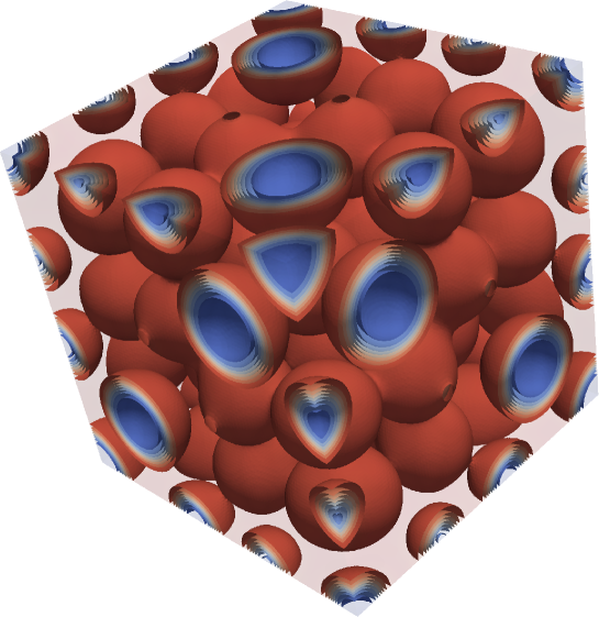
Fig. 1: The final concentration $u$ of the simulation described in section 4. The solution consists of regions of negative material ($u\approx-1$, in blue) embedded within a background of positive material ($u\approx 1$, in red). The figure shows the isosurfaces corresponding to constant values of $u$.

The discretization used standard piecewise linear finite elements for $u$ and $w$, a timestep $\Delta t=\varepsilon^{2}$, a final time $T=300\Delta t$, and an implicitness parameter $\theta=0.5$. The mesh was generated to achieve approximately $2.5\times 10^{5}$ degrees of freedom per core, to investigate how the number of Krylov iterations required to solve (5) varies as the mesh is refined. The preconditioner (7) approximated the action of $A^{-1}$ with ten Chebyshev semi-iterations with SOR preconditioning, and approximated the action of $S^{-1}$ with two Richardson iterations of $\tilde{S}^{-1}$. Each action of $\hat{S}^{-1}$ was in turn approximated with five V-cycles of the BoomerAMG algebraic multigrid solver [7]. GMRES was used as the outer Krylov solver.

Degrees of freedom ($\times 10^{6}$)	Number of cores	Iterations
0.265	1	8.2
2.060	8	8.0
16.24	64	8.0
128.9	512	8.0
1027	4096	8.0

Table 1: Average number of GMRES iterations per Newton step with preconditioner (7) and Schur complement approximation (12) as the problem is weakly scaled. The number of iterations required grows slowly as the mesh is refined.

$\varepsilon$	$\Delta x$	$\Delta t$	Iterations
0.02	0.01	0.0004	8.0
0.01	0.005	0.0001	8.0
0.005	0.0025	0.000025	8.0

Table 2: Average number of GMRES iterations per Newton step with preconditioner (7) and Schur complement approximation (12) as the interfacial thickness $\varepsilon$ is varied (and with it the spatial discretization $\Delta x$ and timestep $\Delta t$). The performance of the preconditioner does not change as $\varepsilon\to 0$.

The essential properties of a good preconditioner are that the Krylov iteration counts are low, they grow slowly (if at all) with mesh refinement, and they are robust to variation in parameters. We therefore examined the average number of Krylov iterations required per Newton step in two numerical experiments: in the the first, all parameters were fixed, and only the mesh was refined; in the second, the interfacial thickness $\varepsilon$ was reduced, and with it the spatial discretisztion (to resolve the interface) and the temporal discretization (to retain stability). The experiments were conducted on Hexagon, a Cray XE6m-200 hosted at the University of Bergen, and ARCHER, a Cray XC30 hosted at the University of Edinburgh.

The results of the first experiment are shown in Table 1. The average number of Krylov iterations per Newton step remains very close to 8, even as the number of degrees of freedom is increased by four orders of magnitude. The results of the second experiment are shown in Table 2. The average number of Krylov iterations required per Newton step does not vary as $\varepsilon\to 0$.

5 Conclusions

We have presented a new preconditioner for the Ohta–Kawasaki equations that model diblock copolymer melts. An approximation to the Schur complement was derived using a matching strategy. The preconditioner proposed yields mesh independent convergence, is robust to changes in interfacial thickness if a timestep criterion is satisfied, and requires no reassembly or reconstruction between Newton steps. This enables the solution of very fine discretizations with billions of degrees of freedom.

References

- [1] B. Benešová, C. Melcher, and E. Süli, An implicit midpoint spectral approximation of nonlocal Cahn–Hilliard equations, SIAM J. Num. Anal., 52 (2014), pp. 1466–1496.
- [2] J. Bosch, D. Kay, M. Stoll, and A. Wathen, Fast solvers for Cahn–Hilliard inpainting, SIAM J. Imaging Sci., 7 (2014), pp. 67–97.
- [3] R. Choksi, M. A. Peletier, and J. F. Williams, On the phase diagram for microphase separation of diblock copolymers: an approach via a nonlocal Cahn–Hilliard functional, SIAM J. Appl. Math., 69 (2009), pp. 1712–1738.
- [4] G. H. Golub and R. S. Varga, Chebyshev semi-iterative methods, successive over-relaxation iterative methods, and second order Richardson iterative methods, Part I, Numer. Math., 3 (1961), pp. 147–156.
- [5] , Chebyshev semi-iterative methods, successive over-relaxation iterative methods, and second order Richardson iterative methods, Part II, Numer. Math., 3 (1961), pp. 157–168.
- [6] A. Greenbaum, V. Pták, and Z. Strakoš, Any nonincreasing convergence curve is possible for GMRES, SIAM J. Matrix Anal. Appl., 17 (1996), pp. 465–469.
- [7] V. E. Henson and U. M. Yang, BoomerAMG: A parallel algebraic multigrid solver and preconditioner, Appl. Numer. Math., 41 (2002), pp. 155–177.
- [8] I. C. F. Ipsen, A note on preconditioning nonsymmetric matrices, SIAM J. Sci. Comput., 23 (2001), pp. 1050–1051.
- [9] A. Logg, K. A. Mardal, G. N. Wells, et al., Automated Solution of Differential Equations by the Finite Element Method, Springer, 2011.
- [10] M. F. Murphy, G. H. Golub, and A. J. Wathen, A note on preconditioning for indefinite linear systems, SIAM J. Sci. Comput., 21 (2000), pp. 1969–1972.
- [11] T. Ohta and K. Kawasaki, Equilibrium morphology of block copolymer melts, Macromolecules, 19 (1986), pp. 2621–2632.
- [12] Q. Parsons, Numerical Approximation of the Ohta–Kawasaki Functional, master’s thesis, University of Oxford, Oxford, UK, 2012.
- [13] J. W. Pearson and A. J. Wathen, A new approximation of the Schur complement in preconditioners for PDE-constrained optimization, Numer. Lin. Alg. Appl., 19 (2012), pp. 816–829.
- [14] Y. Saad and M. Schultz, GMRES: a generalized minimal residual algorithm for solving nonsymmetric linear systems, SIAM J. Sci. Stat. Comput., 7 (1986), pp. 856–869.
- [15] A. J. Wathen and T. Rees, Chebyshev semi-iteration in preconditioning for problems including the mass matrix, Electron. Trans. Numer. Anal., 34 (2009), pp. 125–135.