OGLE-2014-BLG-0257L: A Microlensing Brown Dwarf Orbiting a Low-mass M Dwarf

Abstract

In this paper, we report the discovery of a binary composed of a brown dwarf and a low-mass M dwarf from the observation of the microlensing event OGLE-2014-BLG-0257. Resolution of the very short-lasting caustic crossing combined with the detection of subtle continuous deviation in the lensing light curve induced by the Earth’s orbital motion enable us to precisely measure both the Einstein radius $\theta_{\rm E}$ and the lens parallax $\pi_{\rm E}$, which are the two quantities needed to unambiguously determine the mass and distance to the lens. It is found that the companion is a substellar brown dwarf with a mass $0.036\pm 0.005\ M_{\odot}$ ($37.7\pm 5.2\ M_{\rm J}$) and it is orbiting an M dwarf with a mass $0.19\pm 0.02\ M_{\odot}$. The binary is located at a distance $1.25\pm 0.13$ kpc toward the Galactic bulge and the projected separation between the binary components is $0.61\pm 0.07$ AU. The separation scaled by the mass of the host is $3.2\ {\rm AU}/M_{\odot}$. Under the assumption that separations scale with masses, then, the discovered brown dwarf is located in the zone of the brown dwarf desert. With the increasing sample of brown dwarfs existing in various environments, microlensing will provide a powerful probe of brown dwarfs in the Galaxy.

1. Introduction

Since the first discoveries of Teide 1 (Rebolo et al., 1995) and Gliese 229B (Nakajima et al., 1995) in 1995, the last two decades have witnessed a wealth of brown dwarf (BD) discoveries. In the archives “http://DwarfArchives.org” and the one managed by J. Gagne, there are thousands of known objects fall in the temperature regime occupied by brown dwarfs.

Table 1Microlensing brown dwarfs

Lensing event	Lens	Mass		Reference
		Primary	Secondary
OGLE-2006-BLG-277	BD around an M dwarf	$0.10\pm 0.03\ M_{\odot}$	$52\pm 15\ M_{\rm J}$	(1)
MOA-2007-BLG-197	BD around a G-K dwarf	$0.82\pm 0.04\ M_{\odot}$	$41\pm 2\ M_{\rm J}$	(2)
OGLE-2007-BLG-224	Isolated BD	$59\pm 4\ M_{\rm J}$	-	(3)
OGLE-2008-BLG-510	BD around an M dwarf	-	-	(4)
OGLE-2009-BLG-151	Binary system of BDs	$19.1\pm 1\ M_{\rm J}$	$7.9\pm 0.3\ M_{\rm J}$	(5,6)
MOA 2009-BLG-411	BD around an M dwarf	$0.18\pm 0.02\ M_{\odot}$	$53\pm 5\ M_{\rm J}$	(7)
MOA-2010-BLG-073	BD around an M dwarf	$0.16\pm 0.03\ M_{\odot}$	$11.0\pm 2.0\ M_{\rm J}$	(8)
OGLE-2011-BLG-0420	Binary system of BDs	$26.1\pm 1\ M_{\rm J}$	$9.9\pm 0.5\ M_{\rm J}$	(6)
MOA-2011-BLG-104	BD around an M dwarf	$0.18\pm 0.11\ M_{\odot}$	$21\pm 10\ M_{\rm J}$	(9)
MOA-2011-BLG-149	BD around an M dwarf	$0.14\pm 0.02\ M_{\odot}$	$20\pm 2\ M_{\rm J}$	(9)
OGLE-2012-BLG-0358	BD hosting a planet	$23.2\pm 2.0\ M_{\rm J}$	$1.9\pm 0.2\ M_{\rm J}$	(10)
OGLE-2013-BLG-0102	BD around an M dwarf	$0.10\pm 0.01\ M_{\odot}$	$12.6\pm 2.1\ M_{\rm J}$	(11)
OGLE-2013-BLG-0578	BD around an M dwarf	$0.124\pm 0.014\ M_{\odot}$	$33.6\pm 4.2\ M_{\rm J}$	(12)
OGLE-2015-BLG-1268	Isolated BD	$47\pm 7\ M_{\rm J}$	-	(13)

Note. — (1) Park et al. (2013), (2) Ranc et al. (2015), (3) Gould et al. (2009), (4) Bozza et al. (2012), (5) Shin et al. (2012a), (6) Choi et al. (2013), (7) Bachelet et al. (2012), (8) Street et al. (2013), (9) Shin et al. (2012c), (10) Han et al. (2013), (11) Jung et al. (2015), (12) Park et al. (2015), (13) Zhu et al. (2015).

Despite the large number of known BDs, our understanding about their formation processes is still not clear. As a result, there exist various theories including turbulent fragmentation of molecular clouds (Boyd & Whitworth, 2005), fragmentation of unstable accretion disks (Stamatellos et al., 2007), ejection of protostars from prestellar cores (Reipurth & Clarke, 2001), photo-erosion of prestellar cores by nearby very bright stars (Whitworth & Zinnecker, 2004), etc. It may be that these theories apply to different populations of BDs formed under different environments. For comprehensive studies of the formation mechanism, therefore, it is important to have BD samples detected by using various methods that are sensitive to different populations of BDs.

Due to the nature of detecting objects through their gravitational field rather than their radiation, microlensing experiments can enrich BD samples by detecting BDs that are difficult to be detected by other methods such as old and thus faint or dark brown dwarfs. There have been discovery reports of various types of microlensing BDs as listed in Table 1. These samples include an isolated BD (Gould et al., 2009), BD companions to faint stars (Bozza et al., 2012; Shin et al., 2012a, c; Bachelet et al., 2012; Street et al., 2013; Park et al., 2013; Jung et al., 2015; Park et al., 2015; Ranc et al., 2015), BDs hosting planets (Han et al., 2013), and a binary system of BDs (Choi et al., 2013).

Although rapidly increasing, the number of known microlensing BDs is still limited due to the difficulties in detection. The most important obstacle comes from the difficulties in identifying the BD nature of the lens by measuring its mass. For general lensing events, the only observable parameter related to the mass of the lens is the event time scale $t_{\rm E}$. However, the time scale results from the combination of the lens mass, distance, and relative lens-source speed, and thus the mass estimated from $t_{\rm E}$ is highly degenerate.

For the unique measurement of the mass, one needs to measure two additional quantities of the angular Einstein radius $\theta_{\rm E}$ and the lens parallax $\pi_{\rm E}$. The Einstein radius is measured by detecting the effect of the finite source size on the lensing light curve. On the other hand, the lens parallax can be measured by detecting long-term deviations in lensing light curves caused by the deviation of the lens-source relative motion from rectilinear due to the change of the observer’s position induced by the orbital motion of the Earth around the Sun (Gould, 1992). With the measured $\theta_{\rm E}$ and $\pi_{\rm E}$, the lens mass and distance are determined by

$$M={\theta_{\rm E}\over\kappa\pi_{\rm E}}\qquad D_{\rm L}={{\rm AU}\over\pi_{\rm E}\theta_{\rm E}+\pi_{\rm S}},$$ (1)

respectively. Here $\kappa=4G/(c^{2}{\rm AU})$, $\pi_{\rm S}={\rm AU}/D_{\rm S}$ is the parallax of the source star located at a distance $D_{\rm S}$ (Gould, 2000).

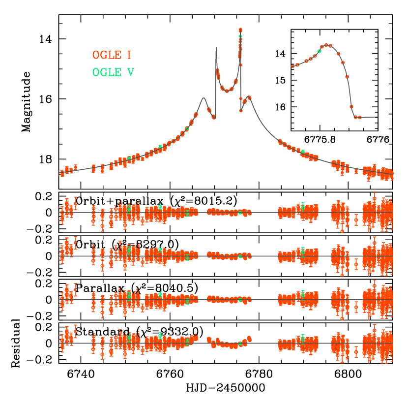
Figure 1.— Light curve of OGLE-2014-BLG-0257. The inset in the top panel shows the enlarged view around the caustic exit. The 4 lower panels show the residuals from the 4 tested models.

For a lensing event produced by a single mass, finite-source effects can be detected only for rare cases of high-magnification events where the lens approaches the source star close enough to pass over the source star surface (Witt & Mao, 1994; Gould, 1994; Nemiroff & Wickramasinghe, 1994; Choi et al., 2012). The chance to measure the lens parallax is also very slim because events produced by low-mass BDs tend to have short time scales while the Earth’s parallactic motion has long-term effects on lensing light curves.

In contrast to single-lens events, the chance to measure lens masses is much higher for events produced by binary lenses. This is first because the majority of binary-lens events are involved with caustic crossings during which finite-source effects are important and thus the chance to measure $\theta_{\rm E}$ is high (Dominik, 1995; Gaudi & Gould, 1999; Gaudi & Petters, 2002; Pejcha & Heyrovský, 2009). Caustics represent the positions on the source plane at which a point-source magnification is infinite and they form a single or multiple closed curves of extended size. For a finite-source, the lensing magnification corresponds to the mean averaged over the source star surface and thus deviates from that of a point source. In addition, although masses of BDs are small, binaries including BDs can be massive and thus events can have time scales long enough for one to measure $\pi_{\rm E}$. As a result, most known microlensing BDs were detected through the channel of binary-lens events, e.g. (Shin et al., 2012b).

Another difficulty of microlensing BD detection comes from the fact that BD signals in the lensing light curve do not have distinctive features. For a binary lens with an extreme companion/primary mass ratio $q$ like a planet-star pair, the caustic induced by the companion is very tiny and the signal of the companion appears as a distinctive short-term anomaly that is superposed on the smooth and symmetric lensing light curve of the primary (Gaudi, 2012). For BD companions with mass ratios $q\sim 0.1$, the size of the induced caustic can be as large as those induced by roughly equal-mass binaries. As a result, it is difficult to immediately notice that the mass of the companion is in the regime of BDs and thus identifying BD companions requires complex procedure of modeling observed light curves.

In this paper, we report the discovery of a BD that is bound to a low-mass star. The BD nature of the companion is identified from the mass measurement, which is possible due to the resolution of a very short-term caustic crossing combined with the detection of a subtle long-term deviation in the lensing light curve induced by the Earth’s orbital motion.

2. Observation and data

The binary system was detected from the observation of a microlensing event OGLE-2014-BLG-0257. The event occurred on a star that lies toward the Galactic Bulge field with equatorial and Galactic coordinates $(\alpha,\delta)_{\rm J2000}=(18^{\rm h}01^{\rm m}47.79^{\rm s},-28^{\circ}15^{\prime}43.2^{\prime\prime})$ and $(l,b)_{\rm J2000}=(2.38^{\circ},-2.72^{\circ})$, respectively. The lensing-induced brightening of the star was first noticed in April, 2014 by the Optical Gravitational Lensing Experiment (OGLE-IV: Udalski et al., 2015) survey that is conducted using the 1.3-m Warsaw telescope located at the Las Campanas Observatory in Chile. In Figure 1, we present the event light curve which shows a typical binary-lensing feature of caustic-crossing spikes with a “U“-shaped trough between them. There also exist two bumps that occurred before and after the caustic crossings.

With the progress of the event, it was noticed that the magnification of the lensed star (source) flux was high. Since high-magnification events are sensitive to planetary companions to lenses (Griest & Safizadeh, 1998), a second alert was issued to the microlensing community on April, 18 (${\rm HJD}\sim 2456765$) for intensive follow-up observation. On April 23 (${\rm HJD}\sim 2456770$), a strong anomaly from a single lensing light curve was detected. Such an anomaly is usually associated with a caustic formed by a binary lens. Caustics form closed curves and thus caustic crossings of a source star occur in pairs, i.e. caustic entrance and exit. Since resolving caustic crossings is important to detect finite-source effects and thus to measure the Einstein radius of the lens, another alert was issued. Despite the successive alerts, immediate follow-up observation could not be done since the anomaly occurred during the early Bulge season when the time window of the bulge visibility was narrow and thus telescopes for follow-up observations were not fully operational. Fortunately, the source star was located in the field toward which stars were monitored with a very high cadence ($\gtrsim 3\ {\rm hr}^{-1}$) and thus the caustic exit was densely resolved despite the short duration ($\sim 3.5$ hours) of the caustic crossing. See the inset in the upper panel of Figure 1, for the enlarged caustic-crossing part of the light curve.

After the caustic exit, there was another bump induced by the source star’s approach close to a cusp of the caustic. From the analyses of the light curve conducted after the second bump, it was noticed that the mass ratio between the binary lens components is $q\sim 0.1$ – 0.2, indicating that the mass of the companion is very low. From continued analyses conducted with the progress of the event, it was also noticed that long-term higher-order effects were needed to precisely describe the observed light curve. The event lasted for about $\sim 3$ months before it returned to its baseline magnitude $I\sim 19$.

In the analysis, we use 8031 OGLE $I$-band data points and 107 $V$-band data points. Photometry of data were conducted by using the customized pipeline (Udalski, 2003) that is based on the Difference Imaging Analysis code developed by Woźniak (2000). For the use of analysis, we readjust the flux measurement uncertainties of each data set by first adding a quadratic term to make the cumulative $\chi^{2}$ distribution ordered by magnifications approximately linear and then rescaling the uncertainties so that $\chi^{2}$ per degree of freedom (dof) becomes unity for the best-fit model.

Table 2Lensing parameter

Parameter	Standard	Parallax		Orbital	Orbital + Parallax
		$u_{0}>0$	$u_{0}<0$		$u_{0}>0$	$u_{0}<0$
$\chi^{2}$	9332.0	8040.5	8044.1	8297.0	8015.2	8025.4
$t_{0}$ (HJD’)	$6774.233\pm 0.021$	$6774.274\pm 0.017$	$6774.255\pm 0.017$	$6774.206\pm 0.018$	$6774.314\pm 0.019$	$6774.321\pm 0.019$
$u_{0}$ ($10^{-2}$)	$0.83\pm 0.01$	$0.78\pm 0.01$	$-0.82\pm 0.01$	$0.92\pm 0.01$	$0.81\pm 0.02$	$-0.80\pm 0.01$
$t_{\rm E}$ (days)	$68.30\pm 0.11$	$77.81\pm 0.23$	$74.80\pm 0.56$	$66.05\pm 0.36$	$77.93\pm 1.40$	$78.73\pm 1.11$
$s$	$0.44\pm 0.01$	$0.42\pm 0.01$	$0.43\pm 0.01$	$0.43\pm 0.01$	$0.43\pm 0.01$	$0.43\pm 0.01$
$q$	$0.22\pm 0.01$	$0.20\pm 0.01$	$0.21\pm 0.01$	$0.25\pm 0.01$	$0.19\pm 0.01$	$0.18\pm 0.01$
$\alpha$ (rad)	$3.116\pm 0.001$	$3.132\pm 0.001$	$-3.133\pm 0.001$	$3.130\pm 0.001$	$3.132\pm 0.001$	$-3.132\pm 0.001$
$\rho$ ($10^{-3}$)	$0.61\pm 0.01$	$0.52\pm 0.01$	$0.54\pm 0.01$	$0.61\pm 0.01$	$0.53\pm 0.01$	$0.520\pm 0.01$
$\pi_{{\rm E},N}$	-	$0.71\pm 0.02$	$-0.73\pm 0.02$	- -	$0.59\pm 0.06$	$-0.76\pm 0.06$
$\pi_{{\rm E},E}$	-	$-0.11\pm 0.01$	$-0.20\pm 0.01$	- -	$-0.13\pm 0.01$	$-0.22\pm 0.01$
$ds/dt$ (${\rm yr}^{-1}$)	-	-	-	$-0.38\pm 0.04$	$0.19\pm 0.05$	$0.25\pm 0.05$
$d\alpha/dt$ (${\rm yr}^{-1}$)	-	-	-	$1.99\pm 0.07$	$0.78\pm 0.25$	$-0.09\pm 0.22$

Note. — ${\rm HJD}^{\prime}={\rm HJD}-2450000$.

3. Modeling

The basic description of a binary-lensing light curve requires seven lensing parameters: $t_{0}$, $u_{0}$, $\alpha$, $t_{\rm E}$, $s$, $q$, and $\rho$. The first four of these parameters describe the source trajectory with respect to the lens: $t_{0}$ is the time of the source star’s closest approach to a reference position in the binary lens, $u_{0}$ is the separation between the source and the reference position at $t_{0}$, $\alpha$ is the angle between the source trajectory and the binary axis, and $t_{\rm E}$ is the time scale required for the source to cross the Einstein radius corresponding to the total mass of the binary. For a reference position on the lens plane, we use the center of mass of the binary lens. Two other parameters describe the binary lens: $s$ is the projected separation normalized to $\theta_{\rm E}$, and $q$ is the mass ratio of the lens components. The last basic parameter, $\rho$, is the source radius normalized to $\theta_{\rm E}$. The normalized source radius is needed to describe the caustic-crossing part of the light curve that is affected by finite-source effects.

The basic features of binary lensing light curves are determined by the size and shape of the caustic, which depends on $s$ and $q$, and the source trajectory with respect to the caustic, which depends on $\alpha$. In the initial modeling run, we therefore explore the $(s,q,\alpha)$ parameter space by conducting a grid search, while the other parameters are searched for by minimizing $\chi^{2}$. For the $\chi^{2}$ minimization, we use the Markov Chain Monte Carlo (MCMC) method. From a $\chi^{2}$ map in the $(s,q,\alpha)$ space obtained from this initial run, we identify the approximate locations of the local minima. We then perform a $\chi^{2}$ optimization using all parameters at each local minima and refine the solution. Finally, we identify a global minimum by comparing $\chi^{2}$ values of the individual local minima. The grid search is important to identify the existence of degenerate solutions which result in similar light curves despite the combinations of dramatically different parameters.

For the computation of finite-source lensing magnifications around the caustic crossings, we use the numerical ray-shooting method. In this process, we consider limb-darkening effects of the source star by modeling its surface brightness profiles as $S_{\lambda}\propto 1-\Gamma_{\lambda}(1-3\cos\phi/2)$, where $\Gamma_{\lambda}$ is the linear limb-darkening coefficient and $\phi$ is the angle between the light of sight toward the center of the source and the normal to the source surface (Albrow et al., 1999). From the de-reddened color and brightness, we find that the source is an F-type main sequence (see section 4 for more details) and adopt a limb-darkening coefficient $\Gamma_{I}=0.37$ from the catalog of Claret (2000). In the grid search, we use the map-making method (Dong et al., 2006), where a magnification map for a given $(s,q)$ is constructed to produce many light curves resulting from different source trajectories.

We identify two local minima in the close ($s<1$) and wide ($s>1$) binary regimes resulting from the well known close/wide binary degeneracy (Dominik, 1999; Bozza, 2000; An, 2005). However, the degeneracy is not severe and the close binary solution provides a better fit with a significant confidence level ($\Delta\chi^{2}\gtrsim 400$). From the modeling run based on the basic parameters (standard model), we find that the event was produced by a close binary with a projected separation $s\sim 0.4$ and a mass ratio $q\sim 0.2$.

Although the standard model explains the main features of the light curve, it is found that there exist noticeable residuals lasting for $\sim 20$ days from the first bump through the caustic-crossing feature to the second bump. See the residual from the standard model at the bottom panel of Figure 1. These residuals may indicate the need to consider higher-order effects. It is known that such a continuous deviation can be caused by either the orbital motion of the Earth around the Sun (“parallax effect”: Refsdal, 1966; Gould, 1992) and/or the change of the lens position caused by the orbital motion of the lens (“lens orbital effect”: Albrow et al., 2000; Dominik, 1998). In order to check these higher-order effects, we test additional models. In the “parallax” and “orbital” models, we consider the parallax and lens-orbital effects, respectively. In the “orbital+parallax” model, we consider both higher-order effects. Consideration of the parallax effect requires to include two additional parameters $\pi_{{\rm E},N}$ and $\pi_{{\rm E},E}$, that are the two components of the lens parallax vector $\mbox{\boldmath$\pi$}_{\rm E}$ projected onto the sky along the north and east equatorial coordinates, respectively. To first-order approximation, the lens-orbital effects are described by two parameters $ds/dt$ and $d\alpha/dt$, that are the change rates of the projected binary separation and the source trajectory angle, respectively. We measure the parallax parameters with respect to the reference time that coincides with $t_{0}$.

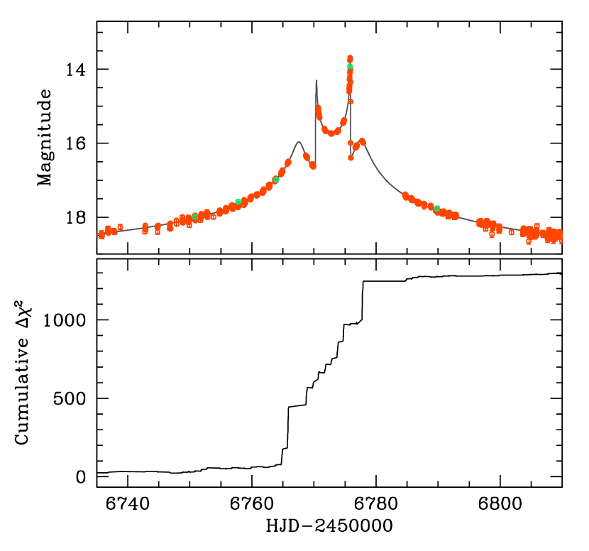
Figure 2.— Cumulative distribution of $\chi^{2}$ difference between the best-fit (orbital+parallax) and the standard binary models.

It is known that a pair of parallax solutions with $u_{0}>0$ and $u_{0}<0$ result in similar light curves due to the mirror symmetry of the source trajectory with respect to the binary axis (Skowron et al., 2011). This so-call “ecliptic degeneracy” is important especially for events that occur on source stars located near the ecliptic plane. The source star of OGLE-2014-BLG-0257 is located just $4.8^{\circ}$ away from the ecliptic plane and thus this degeneracy might be important. We therefore consider both $u_{0}>0$ and $u_{0}<0$ solutions whenever we consider parallax effects. We note that the pair of the two solutions resulting from the ecliptic degeneracy have similar lensing parameters except for the opposite signs of $u_{0}$, $\alpha$, $\pi_{{\rm E},N}$, and $d\alpha/dt$.

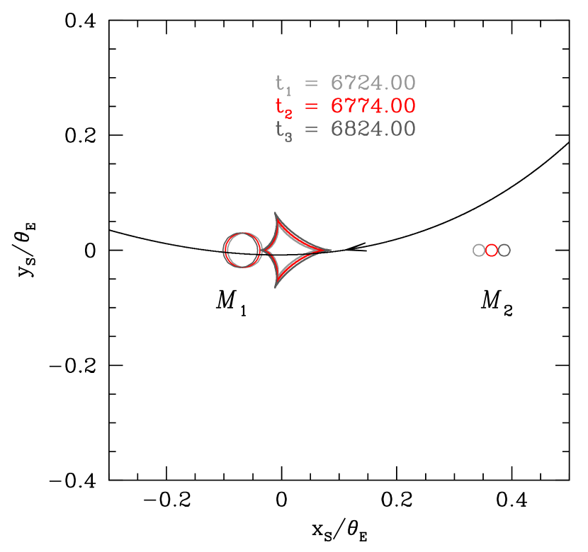
Figure 3.— Source trajectory (curve with an arrow) with respect to the caustic (cuspy closed figure). The two empty circles marked by $M_{1}$ and $M_{2}$ represent the positions of the binary lens components, where $M_{1}>M2$. We note that the positions of the lens components and the caustic vary in time due to the orbital motion of the binary lens and thus we mark locations of the lens components and the caustic at three different times that are marked in the panel. The abscissa is parallel with the binary axis and all lengths are normalized to the angular Einstein radius corresponding to the total mass of the binary, $\theta_{\rm E}$.

In Table 2, we present solutions of the lensing parameters for the tested models along with the $\chi^{2}$ values of the fits. The uncertainties of the individual parameters are estimated based on the distributions of points on the MCMC chain. It is found that the higher-order effects significantly improve the fit. When the parallax and orbital effects are separately considered, the fit improves by $\Delta\chi^{2}=1291.5$ and 1035.0, respectively, compared to the standard model. When both effects are simultaneously considered, the improvement is $\Delta\chi^{2}=1316.8$. See the decrease of the residual for the individual models presented in the lower panels of Figure 1. Considering that (1) the improvement by the parallax effect is significantly greater than the orbital effect and (2) the $\chi^{2}$ difference between the parallax-only and parallax+orbital models ($\Delta\chi^{2}=25.3$) is minor, we judge that the parallax effect plays a dominant role in the fit improvement. In Figure 2, we present the cumulative distribution of $\Delta\chi^{2}$ of the best-fit model (orbit+parallax model) with respect to the standard model. It shows that the improvement occur during the major anomalies of the bumps and caustic-crossing features. We find that the two solutions caused by the ecliptic degeneracy is quite severe although the $u_{0}>0$ solution is preferred over the $u_{0}<0$ solution by $\Delta\chi^{2}=10.2$. Since this level of $\Delta\chi^{2}$ can often be ascribed to systematics in data, one cannot completely rule out the $u_{0}<0$ solution. However, we note that the lensing parameters of the two solutions are similar except for the signs, and thus the estimated physical parameters are also similar to each other.

Figure 3 shows the geometry of the lens event, where we mark the locations of the binary-lens components ($M_{1}$ and $M_{2}$), the caustic, and the source trajectory with respect to the caustic. We note that the positions of the lens components and the caustic vary in time due to the orbital motion of the binary lens and thus we present locations at three different times that are marked in the panel. It is found that a four-cusp central caustic of a close binary lens is responsible for the anomalous features in the lensing light curve. The spikes were produced by the passage of the source trajectory through the caustic and the two bumps were produced by the approach of the source close to the cusps of the caustic before and after the caustic crossing. Considering that only a curved source trajectory can approach both cusps close enough to produce the two strong bumps, the clear detection of the parallax effect was possible because of the good coverage of the major anomalies. The usefulness of triple-peak (one caustic crossing plus two cusp approaches) events in measuring the lens parallax was pointed out by An & Gould (2001).

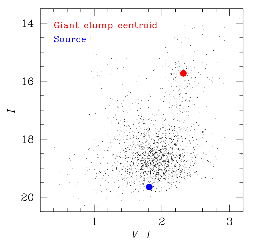
Figure 4.— Locations of the lensed star and the centroid of giant clump in the instrumental color-magnitude diagram.

4. Physical Quantities

Among the two quantities needed for the lens mass measurement, the lens parallax is measured from modeling. The Einstein radius is determined from the combination of the normalized source radius measured from modeling and the angular source radius $\theta_{*}$ by $\theta_{\rm E}=\theta_{*}/\rho$.

We estimate the $\theta_{*}$ from the de-reddened color $(V-I)_{0}$ and brightness $I_{0}$ of the source star. To measure the color and brightness, we first locate the source star in the instrumental color-magnitude diagram of neighboring stars in the same field and then calibrate the color and brightness by using the centroid of the giant clump (GC) as a reference (Yoo et al., 2004). The GC centroid can be used as a standard candle because its de-reddened color and brightness, $(V-I,I)_{0,{\rm GC}}=(1.06,14.35)$ (Bensby et al., 2011; Nataf et al., 2013), are known. Figure 4 shows the locations of the source and GC centroid in the instrumental color-magnitude diagram. The measured offsets in color and magnitude between the source and the GC are $\Delta(V-I)=-0.50$, $\Delta I=3.92$, respectively. Then, the estimated de-reddened color and the brightness of the source star are $(V-I,I)_{0}=(0.56,18.26)$, respectively, indicating that the source is a mid F-type main sequence. We then convert the estimated $(V-I)_{0}$ into $(V-K)_{0}=1.16$ using the color-color relation of Bessell & Brett (1988) and finally determine $\theta_{*}$ using the color-angular radius relation of Kervella et al. (2004). We find that the angular radius of the source star is $\theta_{*}=0.59\pm 0.04\ \mu{\rm as}$. Then the angular Einstein radius corresponding to the best-fit model (orbital+parallax model with $u_{0}>0$) is

$$\theta_{\rm E}={\theta_{*}\over\rho}=1.13\pm 0.08\ {\rm mas}.$$ (2)

Combined with the Einstein time scale estimated from lens modeling, the relative lens-source proper motion is determined as

$$\mu={\theta_{\rm E}\over t_{\rm E}}=5.28\pm 0.38\ {\rm mas}\ {\rm yr}^{-1}.$$ (3)

We note that the values of $\theta_{\rm E}$ and $\mu$ are very similar for the $u_{0}<0$ solution due to the similarity in the measured parameters of $\rho$ and $t_{\rm E}$.

Table 3Physical parameters

Quantity	$u_{0}>0$	$u_{0}<0$
Primary mass	$0.19\pm 0.02\ M_{\odot}$	$0.15\pm 0.02\ M_{\odot}$
Companion mass	$0.036\pm 0.005\ M_{\odot}$	$0.027\pm 0.003\ M_{\odot}$
	$(37.7\pm 5.2\ M_{\rm J})$	$(28.3\pm 3.1\ M_{\rm J})$
Distance to the lens	$1.25\pm 0.13\ {\rm kpc}$	$0.98\pm 0.09\ {\rm kpc}$
Projected separation	$0.61\pm 0.07\ {\rm AU}$	$0.48\pm 0.04\ {\rm AU}$
KE/PE	0.01	0.01

In Table 2, we present the physical parameters of the lens estimated from the measured $\theta_{\rm E}$ and $\pi_{\rm E}$, including the masses of the individual lens components, $M_{1}$ and $M_{2}$, the distance to the lens, $D_{\rm L}$, and the projected separations between the components, $r_{\perp}$. Also presented is the ratio of transverse kinetic to potential energy of the binary system estimated by,

$$\left({\rm KE}\over{\rm PE}\right)_{\perp}={(r_{\perp}/{\rm AU})^{3}\over 8\pi^{2}(M/M_{\odot})}\left[\left({1\over s}{ds/dt\over{\rm yr}^{-1}}\right)^{2}+\left({d\alpha/dt\over{\rm yr}^{-1}}\right)^{2}\right],$$ (4)

where $M=M_{1}+M_{2}$ is the total mass of the binary. For a bound system, the ratio $({\rm KE}/{\rm PE})_{\perp}\leq({\rm KE}/{\rm PE})<1$. The measured ratio is very small and thus satisfies the bound-system check.

From the estimated physical parameters, we find that the lens is a binary composed of a substellar BD with a mass $M_{2}=0.036\pm 0.005\ M_{\odot}$ ($37.7\pm 5.2\ M_{\rm J}$) and a low-mass M dwarf with a mass $M_{1}=0.19\pm 0.02\ M_{\odot}$. The binary is located at a distance $D_{\rm L}=1.25\pm 0.13$ kpc. The projected separation between the lens components is $r_{\perp}=0.61\pm 0.07$ AU. The separation scaled by the mass of the host is $r_{\perp}/M_{1}=3.2\ {\rm AU}/M_{\odot}$. Under the assumption that separations scale with masses, then, the discovered BD is located in the zone of brown-dwarf desert where BDs are rare.

The lens masses estimated from the $u_{0}<0$ solution ($M_{1}=0.15\pm 0.02\ M_{\odot}$ and $M_{2}=0.027\pm 0.003\ M_{\odot}$) are slightly smaller than those estimated from the $u_{0}>0$ solution due to the smaller value of the measured lens parallax. We note, however, that the difference does not affect the nature of the lens (a BD around a M dwarf).

5. Summary

Microlensing provides a powerful probe to study faint or dark objects since these objects can be studied independent of their emitted radiation. By taking advantage of the method, we discovered a brown dwarf orbiting a faint star by analyzing the light curve of the gravitational microlensing event OGLE-2014-BLG-0257. Dense resolution of the short-lasting caustic crossing combined with the detection of subtle deviation induced by parallax effects, we were able to measure both the Einstein radius and the lens parallax. This enabled us to unambiguously determine the physical parameters of the lens system including the mass, distance, and projected separation. It was found that the lens is a binary composed of a brown dwarf and a low-mass star. It was also found that the brown dwarf companion is located in the zone of the brown dwarf desert.

Appendix A Xallarap Effects

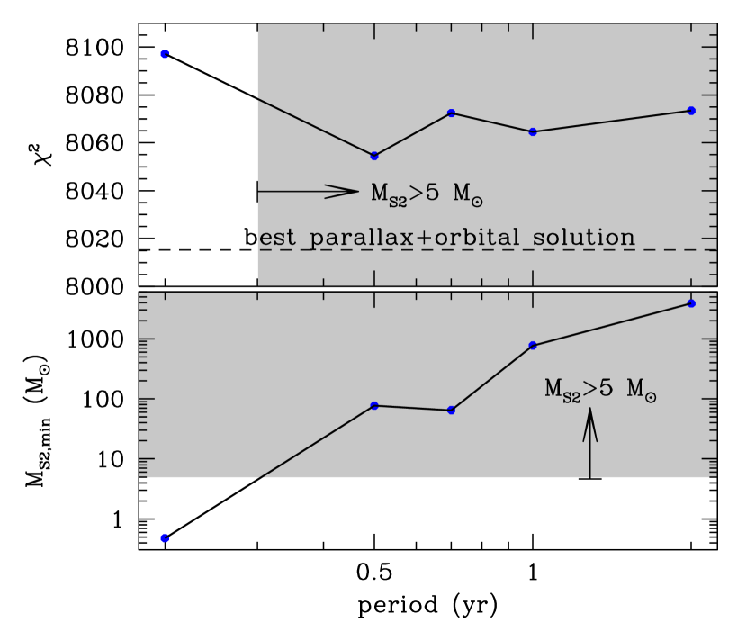
Figure 5.— Upper panel: $\chi^{2}$ distribution of the xallarap fit with respect to the orbital period. Lower panel: distribution of the lower mass limit of the source companion. The dashed line in the upper panel represents the $\chi^{2}$ value of the best-fit orbital + parallax model. The shaded areas represent the regions where the estimated minimum mass of the source companion is greater than $5\ M_{\odot}$.

It is known that long-term deviations in lensing light curves can also be produced by the orbital motion of the source star because it is possible for the source orbital motion to mimic parallax effects (Smith et al., 2003; Poindexter et al., 2005). This effect is often referred to as “xallarap effect”, where xallarap is parallax spelled in reverse. We investigate whether the observed long-term deviation can be explained by xallarap effects rather than parallax effects.

In order to consider xallarap effects, one need 5 additional parameters. These parameters include the orbital period $P$, the phase angle and inclination of the orbit, and the north and east components of the xallarap vector, $\xi_{{\rm E},N}$ and $\xi_{{\rm E},E}$. See details about the parameters in Dong et al. (2009). The magnitude of the xallarap vector $\xi=(\xi_{{\rm E},N}^{2}+\xi_{{\rm E},E}^{2})^{1/2}$ corresponds to the major axis of the orbit with respect to the center of mass, $a_{\rm S}$, normalized to the projected Einstein radius onto the source plane, $\hat{r}_{\rm E}$, i.e.

$$\xi_{\rm E}={a_{\rm S}\over\hat{r}_{\rm E}}={a_{\rm S}\over D_{\rm S}\theta_{\rm E}},$$ (A1)

where $D_{\rm S}$ is the distance to the source. The value $a_{\rm S}$ is related to the semi-major axis of the orbit by $a_{\rm S}=aM_{{\rm S}2}/(M_{{\rm S}1}+M_{{\rm S}2})$, where $M_{{\rm S}1}$ and $M_{{\rm S}2}$ are the masses of the binary source components. With equation (A1) combined with the Kepler’s third law, the mass of the source companion is expressed in terms of $\xi_{\rm E}$ as

$$M_{{\rm S}2}={(\xi\hat{r}_{\rm E})^{3}\over P^{2}}\left({M_{{\rm S}1}+M_{{\rm S}2}\over M_{{\rm S}2}}\right)^{2},$$ (A2)

where mass, period, and distance are expressed in $M_{\odot}$, yr, and AU, respectively. From the fact that $(M_{{\rm S}1}+M_{{\rm S}2})/M_{{\rm S}2}>1$, then the the lower mass limit of the source companion is expressed as

$$M_{{\rm S}2,{\rm min}}={(\xi\hat{r}_{\rm E})^{3}\over P^{2}}.$$ (A3)

In the upper panel of Figure 5, we present the distribution of $\chi^{2}$ with respect to the orbital period. In the lower panel, we also present the distribution of the lower mass limit of the source companion estimated by the relation (A3). From the $\chi^{2}$ distribution, it is found that the best xallarap solution provides a fit that is worse than the best orbital + parallax solution by $\chi^{2}=49.4$, which is statistically important. Furthermore, the estimated minimum mass of the source companion for the best-fit xallarap solution is $M_{{\rm S}2}\sim 100\ M_{\odot}$, implying that the solution is physically unlikely. Therefore, we conclude that xallarap effects cannot explain the observed parallax signal.

References

- Albrow et al. (1999) Albrow, M. D., Beaulieu, J.-P., Caldwell, J. A. R., et al. 1999, ApJ, 512, 672
- Albrow et al. (2000) Albrow, M. D., Beaulieu, J.-P., Caldwell, J. A. R., et al. 2000, ApJ, 534, 894
- An (2005) An, J. H. 2005, MNRAS, 356, 1409
- An & Gould (2001) An, J. H., & Gould, A. 2001, ApJ, 563, L111
- Bachelet et al. (2012) Bachelet, E., Fouqué, P., Han, C., et al. 2012, A&A, 547, 55
- Bensby et al. (2011) Bensby, T., Adén, D.; Meléndez, J., et al. 2011, A&A, 533, 134
- Bessell & Brett (1988) Bessell, M. S., & Brett, J. M. 1988, PASP, 100, 1134
- Boyd & Whitworth (2005) Boyd, D. F. A., & Whitworth, A. P. 2005, A&A, 430, 1059
- Bozza (2000) Bozza, V. 2000, A&A, 355, 423
- Bozza et al. (2012) Bozza, V., Dominik, M., Rattenbury, N. J., et al. 2012, MNRAS, 424, 902
- Choi et al. (2012) Choi, J.-Y., Shin, I.-G., Park, S.-Y., et al. 2012, ApJ, 751, 41
- Choi et al. (2013) Choi, J.-Y., Han, C., Udalski, A., et al. 2013, ApJ, 768, 129
- Claret (2000) Claret, A. 2000, A&A, 363, 1081
- Dominik (1995) Dominik, M. 1995, A&AS, 109, 597
- Dominik (1998) Dominik, M. 1998, A&A, 329, 361
- Dominik (1999) Dominik, M. 1999, A&A, 349, 108
- Dong et al. (2006) Dong, S., DePoy, D. L., Gaudi, B. S., et al. 2006, ApJ, 642., 842
- Dong et al. (2009) Dong, S., Gould, A., Udalski, A., et al. 2009, ApJ, 695, 970
- Gaudi (2012) Gaudi, B. S. 2012, ARA&A, 50, 411
- Gaudi & Gould (1999) Gaudi, B. S., & Gould, A. 1999, ApJ, 513, 61
- Gaudi & Petters (2002) Gaudi, B. S., & Petters, A. O. 2002, ApJ, 580, 468
- Gould (1992) Gould, A. 1992, ApJ, 392, 442
- Gould (1994) Gould, A. 1994, ApJ, 421, L71
- Gould (2000) Gould, A. 2000, ApJ, 542, 785
- Gould et al. (2009) Gould, A., Udalski, A., Monard, B., et al. 2009, ApJ, 698, L147
- Griest & Safizadeh (1998) Griest, K., & Safizadeh, N. 1998, ApJ, 500, 37
- Han et al. (2013) Han, C., Jung, Y. K., Udalski, A., et al. 2013, ApJ, 778, 38
- Jung et al. (2015) Jung, Y. K., Udalski, A., Sumi, T., et al. 2015, ApJ, 798, 123
- Kervella et al. (2004) Kervella, P., Thévenin, F., Di Folco, E., & Ségransan, D. 2004, A&A, 426, 297
- Nakajima et al. (1995) Nakajima, T., Oppenheimer, B. R., Kulkarni, S. R., Golimowski, D. A., Matthews, K., & Durrance, S. T. 1995, Nature, 378, 463
- Nataf et al. (2013) Nataf, D. M., Gould, A., Fouqué, P., et al. 2013, ApJ, 769, 88
- Nemiroff & Wickramasinghe (1994) Nemiroff, R. J., & Wickramasinghe, W. A. D. T. 1994, ApJ, 424, L2
- Park et al. (2013) Park, H., Udalski, A., Han, C., et al. 2013, ApJ, 778, 134
- Park et al. (2015) Park, H., Udalski, A., Han, C., et al. 2015, ApJ, 805, 117
- Pejcha & Heyrovský (2009) Pejcha, O., & Heyrovský, D. 2009, ApJ, 690, 1772
- Poindexter et al. (2005) Poindexter, S., Afonso, C., Bennett, D. P., Glicenstein, J.-F., Gould, A., Szymański, M. K., Udalski, A. 2005, ApJ, 633, 914
- Ranc et al. (2015) Ranc, C., Cassan, A., Albrow, M. D., et al. 2015, A&A, 580, 125
- Rebolo et al. (1995) Rebolo, R.; Zapatero Osorio, M. R.; Martín, E. L. 1995, Nature, 377, 129
- Refsdal (1966) Refsdal, S. 1966, MNRAS, 134, 315
- Reipurth & Clarke (2001) Reipurth, B., & Clarke, C. 2001, AJ, 122, 432
- Shin et al. (2012a) Shin, I.-G., Choi, J.-Y., Park, S.-Y., et al. 2012a, ApJ, 746, 127
- Shin et al. (2012b) Shin, I.-G., Han, C., Choi, J.-Y., et al. 2012b, ApJ, 755, 91
- Shin et al. (2012c) Shin, I.-G., Han, C., Gould, A., et al. 2012c, ApJ, 760, 116
- Skowron et al. (2011) Skowron, J., Udalski, A., Gould, A., et al. 2011, ApJ, 738, 87
- Smith et al. (2003) Smith, M. C., Mao, S., & Paczyński, B. 2003, MNRAS, 339, 925
- Stamatellos et al. (2007) Stamatellos, D., Hubber, D. A., & Whitworth, A. P. 2007, MNRAS, 382, L.30
- Street et al. (2013) Street, R. A., Choi, J.-Y., Tsapras, Y., et al. 2013, ApJ, 763, 67
- Udalski (2003) Udalski, A. 2003, Acta Astron., 53, 291
- Udalski et al. (2015) Udalski, A., Szymański, M. K. & Szymański, G. 2015, Acta Astron., 65, 1
- Whitworth & Zinnecker (2004) Whitworth, A. P., & Zinnecker, H. 2004, A&A, 427, 299
- Witt & Mao (1994) Witt, H. J., & Mao, S. 1994, ApJ, 430, 505
- Woźniak (2000) Woźniak, P. R. 2000, Acta Astron., 50, 421
- Yoo et al. (2004) Yoo, J., DePoy, D. L., Gal-Yam, A., et al. 2004, ApJ, 603, 139
- Zhu et al. (2015) Zhu, W., Calchi Novati, S., Gould, A., et al. 2015, ApJ, submitted