A Generalized Labeled Multi-Bernoulli Filter for Maneuvering Targets

Abstract

A multiple maneuvering target system can be viewed as a Jump Markov System (JMS) in the sense that the target movement can be modeled using different motion models where the transition between the motion models by a particular target follows a Markov chain probability rule. This paper describes a Generalized Labelled Multi-Bernoulli (GLMB) filter for tracking maneuvering targets whose movement can be modeled via such a JMS. The proposed filter is validated with two linear and non-linear maneuvering target tracking examples.

I Introduction

Multiple target tracking is the problem of estimating an unknown and time varying number of trajectories from observed data. There are two main challenges in this problem. The first is the time-varying number of targets due to the appearance of new targets and deaths of existing targets, while the second is the unknown association between measurements and targets, which is further confounded by false measurements and missed detections of actual targets [1, 2, 3, 4, 5, 6].

The Bayes optimal approach to the multi-target tracking problem is the Bayes multi-target filter that recursively propagates the multi-target posterior density forward in time [3] incorporating both the uncertainty in the number of objects as well as their states. Under the standard multi-target system model (which takes into account target births,deaths,survivals and detections,misdetections and clutter), the multi-target posterior densities at each time are Generalized Labeled Multi-Bernoulli (GLMB) densities [7]. The $\delta$-GLMB filter [8, 9, 10] is an analytic solution to the multi-target Bayes filter.

While a non-maneuvering target motion can be described by a fixed model, a combination of motion models that characterise different maneuvers may be needed to describe the motion of a maneuvering target.Tracking a maneuvering target in clutter is a challenging problem and is the subject of numerous works [11, 12, 13, 1, 2, 14, 15, 16, 18, 24, 25, 26]. Tracking multiple maneuvering targets involves jointly estimating the number of targets and their states at each time step in the presence of noise, clutter, uncertainties in target maneuvers, data association and detection. As such, this problem is extremely challenging in both theory and implementation.

The jump Markov system (JMS) or multiple models approach has proven to be an effective tool for single maneuvering target tracking [12, 13, 18, 24, 25, 26]. In this approach, the target can switch between a set of models in a Markovian fashion. The interacting multiple model(IMM) and variable-structure IMM (VS-IMM) estimators [1, 2, 14, 15, 16] are two well known single-target filtering algorithms for maneuvering targets. The number of modes in the IMM is kept fixed, whereas in the VS-IMM the number of modes are adaptively selected from a fixed set of modes for improved estimation accuracy and computational efficiency.

A Probability Hypothesis Density (PHD) filter [17] for maneuvering target tracking was derived in [18] together with a Gaussian mixture implementation and particle implementation. As shown by Mahler in [19], this was the only mathematically valid filter amongst severval PHD (and Cardinalized PHD) filters proposed for jump Markov systems (JMSs) [20],[21]. Recently, multi-Bernoulli and labeled multi-Bernoulli [22], [23] filters were also derived for JMSs in [24, 25, 26]. These filters, however, are only approximate solutions to the Bayes multi-target filter for maneuvering targets, and at present there are no exact solutions in the literature.

In this paper, we propose an analytic solution to the Bayes multi-target filter for maneuvering target tracking using JMSs. Specifically, we extend the GLMB filter to JMSs that can be implemented via Gaussian mixture or sequential Monte Carlo methods. In addition to being an analytic solution and hence more accurate than approximations, the proposed solution outputs tracks or trajectories of the targets, whereas the PHD and (unlabeled) multi-Bernoulli filters do not. The proposed technique is verified via numerical examples.

II Background

We review JMS and the Bayes multi-target tracking filter in this section.

II-A JMS model for maneuvering targets

A JMS consists of a set of parameterised state space models, whose parameters evolve with time according to a finite state Markov chain. An example of a maneuvering target scenario which can be successfully represented using a JMS model is the dynamics of an aircraft, which can fly with a nearly constant velocity motion, accelerated/decelerated motion, and coordinated turn [1, 2]. Under a JMS framework for such a system a target that is moving under a certain motion model at any time step are assumed to follow the same motion model with a certain probability or switch to a different motion model (that belongs to a set of pre-selected motion models) with a certain probability in the next time step.

A Markovian transition probability matrix describes the probabilities with which a particular target changes/retains the motion model in the next time step given the motion model at current time step. Let $\vartheta(r|r^{\prime})$ denote the probability of switching to motion model $r$ from $r^{\prime}$ as given by this markovian transition matrix, in which the sum of the conditional probabilities of all possible motion models in the next time step given the current model adds upto 1, i.e.,

$$\sum_{r\in\mathcal{R}}\vartheta(r|r^{\prime})=1$$ (1)

where $R$ is the (discrete) set of motion models in the system.

Suppose that model $r$ is in effect at time $k$, then the state transition density from $\zeta^{\prime}$, at time $k-1$, to $\zeta$, at time $k$, is denoted by $\phi_{k|k-1}(\zeta|\zeta^{\prime},r)$, and the likelihood of $\zeta$ generating the measurement $z$ is denoted by $\gamma_{k}(z|\zeta,r)$ [1, 2, 35]. Moreover, the joint transition of the state and the motion model assumes the form:

$$f_{k|k-1}(\zeta,r|\zeta^{\prime},r^{\prime})=\phi_{k|k-1}(\zeta|\zeta^{\prime},r)\vartheta(r|r^{\prime}).$$ (2)

In general, the measurement can also depend on the model $r$ and hence the likelihood function becomes $g_{k}(z|\zeta,r)$. Note that by defining the augmented system state as $x=(\zeta,r\mathbf{)}$ a JMS model can be written as a standard state space model.

JMS models are not only useful for tracking maneuvering targets, but are also useful in the estimation of unknown clutter parameters [27, 28].

II-B Bayes multi-target tracking filter

In the Bayes multi-target tracking filter, the state of a target includes an ordered pair of integers $\ell=(k,i)$, where $k$ is the time of birth, and $i$ is a unique index to distinguish targets born at the same time. The label space for targets born at time $k$ is denoted as $\mathbb{L}_{k}$ and the label space for targets at time $k$ (including those born prior to $k$) is denoted as $\mathbb{L}_{0:k}$. Note that $\mathbb{L}_{0:k}=\mathbb{L}_{0:k-1}\cup\mathbb{L}_{k}$, and that $\mathbb{L}_{0:k-1}$ and $\mathbb{L}_{k}$ are disjoint. An existing target at time $k$ has state $\mathbf{x}=(x,\ell)$ consisting of the kinematic/feature $x$ and label $\ell\in\mathbb{L}_{0:k}$. A multi-target state $\mathbf{X}$ (uppercase notation) is a finite set of single-target states.

All information about the multi-target state at time $k$ is contained in $\mathbf{\pi}_{k}$, the posterior density of the multi-target state conditioned on $Z_{1:k}=(Z_{1},...,Z_{k})$, the measurement history upto time $k$, where $Z_{k}$ is the finite set of measurements received at time $k$. The Bayes multi-target tracking filter consists of a prediction step (3) and an update step (4), which propagate the multi-target posterior/filtering density forward in time. Note that the integral in this case is the set integral from finite set statistics [3].

$$\mathbf{\pi}_{k|k-1}(\mathbf{X}_{k})\!=\!\!\int\!\mathbf{f}_{k|k-1}(\mathbf{X}_{k}|\mathbf{X})\mathbf{\pi}_{k-1}(\mathbf{X})\delta\mathbf{X}$$ (3)

$$\mathbf{\pi}_{k}(\mathbf{X}_{k})=\frac{g_{k}(Z_{k}|\mathbf{X}_{k})\mathbf{\pi}_{k|k-1}(\mathbf{X}_{k})}{\int g_{k}(Z_{k}|\mathbf{X})\mathbf{\pi}_{k|k-1}(\mathbf{X})\delta\mathbf{X}}$$ (4)

where $\mathbf{f}_{k|k-1}(\cdot|\cdot)$ denotes the multi-target transition kernel from time $k-1$ to $k$, and $g_{k}(\cdot|\cdot)$ denotes the likelihood function at time $k$. Note that for compactness we omitted dependence on the measurement history from $\mathbf{\pi}_{k|k-1}$ and $\mathbf{\pi}_{k}$. Note that the same multi-target recursion (3)-(4) also holds for multi-target states without labels.

A generic particle implementation of the multi-target Bayes recursions (3)-(4) (for both labeled and unlabeled multi-target states) was given in [29], while analytic approximations for unlabeled multi-target states, such as the PHD, Cardinalized PHD and multi-Bernoulli filters were proposed in [3, 30, 31, 32, 22, 33]. The GLMB filter [7], [8] is an analytic solution to the multi-target Bayes recursions (3)-(4).

III JMS-GLMB filtering

We start this subsection with some notations. For the labels of a multi-target state $\mathbf{X}$ to be distinct, we require $\mathbf{X}$ and the set of labels of $\mathbf{X}$, denoted as $\mathcal{L}(\mathbf{X})$, to have the same cardinality, .i.e. the same number of elements. Hence, we define the distinct label indicator as the function

$$\Delta(\mathbf{X})\triangleq\delta_{|\mathbf{X}|}[|\mathcal{L(}\mathbf{X})|],$$

where $|Y|$ denotes the cardinality of the set $Y$, and $\delta_{n}[m]$ denotes the Kronecker delta. The indicator function is defined as as

$$1_{Y}(x)\triangleq\Big{\{}{}\begin{array}[]{ll}1,&\text{if }x{\in Y}\\ 0,&\text{otherwise }{}\end{array}.$$

For any finite set $Y$, and test function $h\leq 1$, the multi-object exponential is defined by

$$h^{Y}\triangleq\prod_{y\in Y}h(y),$$

with $h^{\emptyset}$ $=1$ by convention. We also use the standard inner production notation

$$\left\langle f,g\right\rangle=\int f(x)g(x)dx,$$

for any real functions $f$ and $g$.

An association map at time $k$ is a function $\theta:\mathbb{L}_{0:k}\rightarrow\{0,1,...,|Z_{k}|\}$ such that $\theta(\ell)=\theta(\ell^{\prime})>0~{}$implies$~{}\ell=\ell^{\prime}$. Such a function can be regarded as an assignment of labels to measurements, with undetected labels assigned to $0$. The set of all such association maps is denoted as $\Theta_{k}$; the subset of association maps with domain $L$ is denoted by $\Theta_{k}(L)$; and $\Theta_{0:k}\triangleq\Theta_{0}\times...\times\Theta_{k}$ denotes the space of association map history.

III-A GLMB filter

In the GLMB filter, the multi-target filtering density at time $k-1$ is a GLMB of the form:

$$\mathbf{\pi}_{k-1}(\mathbf{X})=\Delta(\mathbf{X})\!\!\!\sum_{\xi\in\Theta_{0:k\!-\!1}}\!\!\!\!w_{k-1}^{(\xi)}(\mathcal{L(}\mathbf{X}))[p_{k-1}^{(\xi)}]^{\mathbf{X}},$$ (5)

where each $\xi=(\theta_{0},...,\theta_{k-1})\in\Theta_{0:k-1}$ represents a history of association maps up to time $k-1$; each weight $w_{k-1}^{(\xi)}(L)$ is non-negative with

$$\sum_{L\subseteq\mathbb{L}_{0:k-1}}\sum_{\xi\in\Theta_{0:k-1}}w_{k-1}^{(\xi)}(L)=1,$$

and each $p_{k-1}^{(\xi)}(\cdot,\ell)$ is a probability density.

Given a GLMB filtering density, a tractable suboptimal multi-target estimate is obtained by the following proceedure: determine the maximum a posteriori cardinality estimate $n^{\ast}$ from the cardinality distribution

$$\rho_{k-1}(n)=\sum_{L\subseteq\mathbb{L}_{0:k-1}}\sum_{\xi\in\Theta_{0:k-1}}\delta_{n}[|L|]w_{k-1}^{(\xi)}(L);$$ (6)

determine the label set $L^{\ast}$ and $\xi^{\ast}$ with highest weight $w_{k-1}^{(\xi^{\ast})}(L^{\ast})$ among those with cardinality $n^{\ast}$; determine the expected values of the states from $p_{k-1}^{(\xi^{\ast})}(\cdot,\ell)$, $\ell\in L^{\ast}$ [7].

The GLMB density is a conjugate prior with respect to the standard multi-target likelihood function and is also closed under the multi-target prediction [7]. Under the standard multi-target transition model, if the multi-target filtering density, at the previous time, $\mathbf{\pi}_{k-1}$ is a GLMB of the form (5), then the multi-target prediction density $\mathbf{\pi}_{k|k-1}$ is a GLMB of the form (13) given by [7].

$$\mathbf{\pi}_{k|k-1}(\mathbf{X})=\Delta(\mathbf{X})\!\!\!\sum_{\xi\in\Theta_{0:k-1}}\!\!w_{k|k-1}^{(\xi)}(\mathcal{L(}\mathbf{X}))[p_{k|k-1}^{(\xi)}]^{\mathbf{X}},$$ (7)

where

$$\!\!\!\!\!\!\!\!\!\!w_{k|k\!-\!1\!}^{(\xi)}(L)\!\!\!\! = \!\!\!\!w_{S,k|k-1}^{(\xi)}(L\cap\mathbb{L}_{0:k-1})w_{B,k}(L\cap\mathbb{L}_{k}),$$

$$\!\!\!\!\!\!\!\!\!\!p_{k|k\!-\!1\!}^{(\xi)}(x,\ell)\!\!\!\! = \!\!\!\!1_{\mathbb{L}_{0:k\!-\!1}\!}(\ell)p_{S,k|k\!-\!1\!}^{(\xi)\!}(x,\ell)\!+\!1_{\mathbb{L}_{k}\!}(\ell)p_{B,k}(x,\ell),$$

$$\!\!\!\!\!\!\!\!\!\!w_{S,k|k\!-\!1\!}^{(\xi)}(L)\!\!\!\! = \!\!\!\![\bar{P}_{S,k|k\!-\!1}^{(\xi)}]^{L}\!\sum_{I\supseteq L}[1\!-\!\bar{P}_{S,k|k\!-\!1}^{(\xi)}]^{I\!-\!L}w_{k\!-\!1\!}^{(\xi)}(I),$$

$$\!\!\!\!\!\!\!\!\!\!\bar{P}_{S,k|k\!-\!1\!}^{(\xi)}(\ell)\!\!\!\! = \!\!\!\!\left\langle P_{S,k|k-1}(\cdot,\ell),p_{k-1}^{(\xi)}(\cdot,\ell)\right\rangle,$$

$$\!\!\!\!\!\!\!\!\!\!p_{S,k|k\!-\!1\!}^{(\xi)}(x,\ell)\!\!\!\! = \!\!\!\!\frac{\left\langle P_{S,k|k\!-\!1}(\cdot,\ell)f_{k|k\!-\!1\!}(x|\cdot,\ell),p_{k\!-\!1}^{(\xi)}(\cdot,\ell)\right\rangle}{\bar{P}_{S,k|k-1}^{(\xi)}(\ell)},$$

$$\!\!\!\!\!\!\!\!\!\!P_{S,k|k-1}(x,\ell)\!\!\!\! = \!\!\!\!\text{probability of survival to time }k\text{ of a target }$$

$$\!\!\!\!\text{with previous state }(x,\ell),$$

$$f_{k|k\!-\!1\!}(x|x^{\prime},\ell)\!\!\!\! = \!\!\!\!\text{transition density of feature }x^{\prime}\text{ at time }$$

$$\!\!\!\!k-1\text{ to }x\text{ at time }k\text{ for target with label }\ell\text{, }$$

$$\!\!\!\!\!\!\!\!\!\!w_{B,k}(L)\!\!\!\! = \!\!\!\!\text{probability of targets with labels }L\text{ being }$$

$$\!\!\!\!\text{born at time }k\text{,}$$

$$\!\!\!\!\!\!\!\!\!\!p_{B,k}(x,\ell)\!\!\!\! = \!\!\!\!\text{probability density of the feature }x\text{ of a}$$

$$\!\!\!\!\text{new target born at time }k\text{ with label }\ell\text{.}$$

Moreover, under the standard multi-target measurement model, the multi-target filtering density $\mathbf{\pi}_{k}$ is a GLMB given by

$$\mathbf{\pi}_{k}\!(\mathbf{X})=\Delta\!(\mathbf{X})\!\!\!\!\!\!\sum_{\xi\in\Theta_{0:k\!-\!1}}\sum\limits_{\theta\in\Theta_{k}}\!w_{k}^{\!(\xi,\theta)\!}(\mathcal{L(}\mathbf{X})|Z_{k})[p^{\!(\xi,\theta)\!}(\cdot|Z_{k})]^{\mathbf{X}}\!\!,$$ (8)

where

$$w_{k}^{(\xi,\theta)\!}(L|Z)\!\!\! \propto \!\!\!1_{\Theta_{k}\!(L)}(\theta)[\bar{\Psi}_{Z,k}^{(\xi,\theta)}]^{L}w_{k|k-1}^{(\xi)}(L),$$

$$p_{k}^{\!(\xi,\theta)\!}(x,\ell|Z)\!\!\! = \!\!\!\frac{\Psi_{Z,k}^{(\theta)}(x,\ell)p_{k|k-1}^{(\xi)}(x,\ell)}{\bar{\Psi}_{Z,k}^{(\xi,\theta)}(\ell)}$$

$$\bar{\Psi}_{Z,k}^{(\xi,\theta)}(\ell)\!\!\! = \!\!\!\left\langle\Psi_{Z,k}^{(\theta)}(\cdot,\ell),p_{k|k-1}^{(\xi)}(\cdot,\ell)\right\rangle,$$

$$\Psi_{\{z_{1},...,z_{m}\},k}^{(\theta)}(x,\ell)\!\!\! = \!\!\!\left\{\begin{array}[]{ll}\frac{P_{D,k}(x,\ell)g_{k}(z_{\theta(\ell)}|x,\ell)}{\kappa_{k}(z_{\theta(\ell)})},&\text{if }{\small\theta(\ell)>0}\\ {\small 1-P}_{D,k}{\small(}x{\small,\ell)},&\text{if }{\small\theta(\ell)=0}\end{array}\right.$$

$$P_{D,k}(x,\ell)\!\!\! = \!\!\!\text{probability of detection at time }k$$

$$\!\!\!\text{of a target with state }(x,\ell),$$

$$g_{k}(z|x,\ell)\!\!\! = \!\!\!\text{likelihood that at time }k\text{ target with}$$

$$\!\!\!\text{state }(x,\ell)\text{ generate measurement }z,$$

$$\kappa_{k}\!\!\! =$$ intensity function of Poisson clutter

$$\!\!\!\text{at time }k\text{ }$$

The GLMB recursion above is the first analytic solution to the Bayes multitarget filter. Truncating the GLMB sum is needed to manage the growing the number of components in the GLMB filter [8].

III-B GLMB filter for Manuevering Targets

We define the (labeled) state of a manuevering target to include the kinematic/feature $\zeta$, the motion model index $r$, and the label $\ell$, i.e., $\mathbf{x}=(\zeta,r,\ell)$, which can be modeled as a JMS. Note that the label of each target remains constant throughout it’s life even though it is part of the state vector. Hence the JMS state equations for a target with label $\ell$ are indexed by $\ell$, i.e., $\phi_{k|k-1}^{(\ell)}(\zeta|\zeta^{\prime},r)$ and $\gamma_{k}^{(\ell)}(z|\zeta,r)$. The new state of a surviving target will also be governed by the probability of the target transitioning to that motion model from the previous model in addition to the probability of survival and the relevant state transtition function. Consequently, the joint transition and likelihood function for the state and the model index are given by,

$$f_{k|k-1}(\zeta,r|\zeta^{\prime},r^{\prime},\ell) = \phi_{k|k-1}^{(\ell)}(\zeta|\zeta^{\prime},r)\times\vartheta(r|r^{\prime})$$ (10)

$$g_{k}(z|\zeta,r,\ell) = \gamma_{k}^{(\ell)}(z|\zeta,r)$$ (11)

Substituting (10) and (11) into the GLMB prediction and update equations yields the GLMB filter for maneuvering targets. Note that since $x=(\zeta,r)$

$$\int f(x)dx=\sum_{r\in\mathcal{R}}\int f(\zeta,r)d\zeta.$$

The state extraction is akin to the single model system. To estimate the motion model for each label, we select the motion model that maximizes the marginal probability of that model over the entire density for that label, i.e., for label $\ell$ of component $\xi$, the estimated motion model $\hat{r}$ is given by (12).

$$\hat{r}=\underset{r}{\mbox{argmax}}\;\int p^{(\xi)}(\zeta,r,\ell)d\zeta$$ (12)

III-C Analytic Solution

Consider the special case where the target birth model, motion models and observation model are all linear models with Gaussian noise. Given that the posterior density at time $k-1$ is of the form (5) with $\mathbf{x}=(\zeta,r,\ell)$, the GLMB filter prediction equation can be explicitly written as

$$\mathbf{\pi}_{k|k-1}(\mathbf{X})=\Delta(\mathbf{X})\!\!\!\sum_{\xi\in\Theta_{0:k-1}}\!\!w_{k|k-1}^{(\xi)}(\mathcal{L(}\mathbf{X}))[p_{k|k-1}^{(\xi)}]^{\mathbf{X}},$$ (13)

where

$$\!\!\!\!\!\!\!\!\!\!w_{k|k\!-\!1\!}^{(\xi)}(L)\!\!\!\! = \!\!\!\!w_{S,k|k-1}^{(\xi)}(L\cap\mathbb{L}_{0:k-1})w_{B,k}(L\cap\mathbb{L}_{k}),$$

$$\!\!\!\!\!\!\!\!\!\!p_{k|k\!-\!1\!}^{(\xi)}(\zeta\!,r\!,\ell\!)\!\!\!\! = \!\!\!\!1_{\mathbb{L}_{0:k\!-\!1}\!}(\ell)p_{S,k|k\!-\!1\!}^{(\xi)\!}(\zeta\!,r\!,\ell\!)\!\!+\!\!1_{\mathbb{L}_{k}\!}(\ell)p_{B,k}(\zeta\!,r\!,\ell\!),$$

$$\!\!\!\!\!\!\!\!\!\!w_{S,k|k\!-\!1\!}^{(\xi)}(L)\!\!\!\! = \!\!\!\![\bar{P}_{S,k|k\!-\!1}^{(\xi)}]^{L}\!\sum_{I\supseteq L}[1\!-\!\bar{P}_{S,k|k\!-\!1}^{(\xi)}]^{I\!-\!L}w_{k\!-\!1\!}^{(\xi)}(I),$$

$$\!\!\!\!\!\!\!\!\!\!\bar{P}_{S,k|k\!-\!1\!}^{(\xi)}(\ell)\!\!\!\! = \!\!\!\!\sum_{r\in R}\bar{P}_{S,k|k\!-\!1\!}^{(\xi)}(r,\ell),$$

$$\!\!\!\!\!\!\!\!\!\!\bar{P}_{S,k|k\!-\!1\!}^{(\xi)}(r,\ell)\!\!\!\! = \!\!\!\!\left\langle P_{S,k|k-1}(\cdot,r,\ell),p_{k-1}^{(\xi)}(\cdot,r,\ell)\right\rangle,$$

$$\!\!\!\!\!\!\!\!\!\!p_{S,k|k\!-\!1\!}^{(\xi)}(\zeta,r,\ell)\!\!\!\! = \!\!\!\!\!\!\frac{\underset{r^{\prime}\in R}{\sum}\!\!\!\left\langle\!\!P_{S,k|k\!-\!1}(\cdot,\ell)f_{k|k\!-\!1\!}(\!\zeta,r|\!\cdotp\!,r^{\prime}\!,\ell),p_{k\!-\!1}^{(\xi)}(\!\cdot\!,\!\ell)\!\!\right\rangle\!\!}{\bar{P}_{S,k|k-1}^{(\xi)}(\ell)},$$

$$\!\!\!\!\!\!\!\!\!\!P_{S,k|k-1}(\zeta,r,\ell)\!\!\!\! = \!\!\!\!\text{probability of survival to time }k\text{ of a }$$

$$\!\!\!\!\text{target with previous labeled state }(\zeta,r,\ell),$$

$$f_{k|k\!-\!1\!}(\zeta,r|\zeta^{\prime},r^{\prime},\ell)\!\!\!\! = \!\!\!\mathcal{N}(\zeta;F^{(r)}\zeta^{\prime},Q_{F}^{(r)})\times\vartheta(r|r^{\prime})$$

$$F^{(r)}\!\!\! = \!\!\!\text{state transition matrix of motion mode\!l }r,$$

$$Q_{F}^{(r)}\!\!\! = \!\!\!\text{covariance matrix of motion model }r,$$

$$\!\!\!\!\!\!\!\!\!\!w_{B,k}(L)\!\!\!\! = \!\!\!\!\text{probability of targets with labels }L\text{ being }$$

$$\!\!\!\!\text{born at time }k,$$

$$\!\!\!\!\!\!\!\!\!\!p_{B,k}(\zeta,r,\ell)\!\!\!\! = \!\!\!\!\mathcal{N}(\zeta;m^{(i)},Q_{B}^{(i)})\times\vartheta^{(i)}(r)$$

$$\vartheta^{(i)}(r) =$$ probability that a target born at birth

$$\!\!\!\!\text{ region }i\text{ possesses motion model }r,$$

$$m^{(i)}\!\!\! = \!\!\!\text{mean of birth region }i,$$

$$Q_{B}^{(i)}\!\!\! = \!\!\!\text{covariance of birth region }i,$$

Moreover, GLMB update formula can be written explicitly as

$$\mathbf{\pi}_{k}\!(\mathbf{X})=\Delta\!(\mathbf{X})\!\!\!\!\!\!\sum_{\xi\in\Theta_{0:k\!-\!1}}\sum\limits_{\theta\in\Theta_{k}}\!w_{k}^{\!(\xi,\theta)\!}(\mathcal{L(}\mathbf{X})|Z_{k})[p^{\!(\xi,\theta)\!}(\cdot|Z_{k})]^{\mathbf{X}}\!\!,$$ (14)

where

$$w_{k}^{(\xi,\theta)\!}(L|Z)\!\!\! \propto \!\!\!1_{\Theta_{k}\!(L)}(\theta)[\bar{\Psi}_{Z,k}^{(\xi,\theta)}]^{L}w_{k|k-1}^{(\xi)}(L),$$

$$p_{k}^{\!(\xi,\theta)\!}(\zeta,r,\ell|Z)\!\!\!\! = \!\!\!\frac{\Psi_{Z,k}^{(\theta)}(\zeta,r,\ell)p_{k|k-1}^{(\xi)}(\zeta,r,\ell)}{\bar{\Psi}_{Z,k}^{(\xi,\theta)}(\ell)}$$

$$\bar{\Psi}_{Z,k}^{(\xi,\theta)}(\ell)\!\!\!\! = \!\!\!\sum_{r\in R}\left\langle\Psi_{Z,k}^{(\theta)}(\cdotp,r,\ell),p_{k|k-1}^{(\xi)}(\cdot,r,\ell)\right\rangle,$$

$$\Psi_{\{z_{1},...,z_{m}\},k}^{(\theta)}(\zeta,r,\ell)\!\!\!\! = \!\!\!\!\left\{\begin{array}[]{ll}\!\!\!\frac{P_{D,k}(\zeta,r,\ell)g_{k}(z_{\theta(\ell)}|\zeta,r,\ell)}{\kappa_{k}(z_{\theta(\ell)})},&\!\!\!\!\text{if }{\small\theta(\ell)>0}\\ \!\!\!{\small 1-P}_{D,k}{\small(}\zeta,r{\small,\ell)},&\!\!\!\!\text{if }{\small\theta(\ell)=0}\end{array}\right.$$

$$P_{D,k}(\zeta,r,\ell)\!\!\! = \!\!\!\!\text{probability of detection at time }k$$

$$\!\!\!\text{of a target with state }(\zeta,r,\ell),$$

$$g_{k}(z|\zeta,r,\ell)\!\!\! = \!\!\!\!\mathcal{N}(z;H^{(r)}\zeta,Q_{H}^{(r)})$$

$$\kappa_{k}\!\!\! = \!\!\!\!\text{intensity function of Poisson clutter},$$

$$H^{(r)}\!\!\! =$$ likelihood matrix for targets

$$\!\!\!\!\text{moving under motion model r},$$

$$Q_{H}^{(r)}\!\!\! =$$ covariance matrix of likelihood for

$$\!\!\!\!\text{targets \negthinspace moving \negthinspace under \negthinspace motion \negthinspace model r}.$$

For mildly non-linear motion models and measurement models, the unscented Kalman Filter (UKF) [35, 34] can been utilized for predicting and updating each Gaussian component in the mixture forward. Alternatively, instead of a making use of a Gaussian mixture to represent the posterior density of each track in a hypothesis, a particle filter can be employed. Instead of a Gaussian mixture, the density is represented using a set of particles which are propagated forward under the different motion models with adjusted weights for each particle. As in the case of the Gaussian mixture, the number of particles in the density increase by threefold during each prediction forward. Thus resampling needs to be carried out to discard particles with negligible weights and keep the total count of particles in control.

III-D Implementation Issues

In the above solution it is evident that the posterior density for each track is a Gaussian mixture, with each mixture component relating to one of the motion models present. For a particular track, at each new time step the posterior is predicted forward for all motion models present in the system, thereby generating a new Gaussian mixture. The weight of each new component will be the weight of the parent component multiplied by the probability of switching to the corresponding motion model. As a result the number of mixture components escalates exponentially. Hence extensive pruning and merging must be carried out for each track in each GLMB hypothesis after the update step to keep the computation managable.

IV Simulation Results

In this section we demonstrate the use of the proposed JMS-GLMB solution via two multiple manuevering target tracking examples.

Linear Example: The kinematic state of each target in this example consists of cartesian x and y coordinates and their respective velocities. $T=5s$ is the sampling interval. The observation area is a [-60, 60] $\times$ [-60, 60] $km^{2}$ area. The JMS used in the simulation consists of three types of motion models viz. constant velocity, right turn (coordinated turn with a $3^{\circ}$ angle), and left turn (coordinated turn with a $-3^{\circ}$ angle). The state transition matrices for the three models are obtained via substituting $\omega=0$, $\omega=5\pi/180$ and $\omega=-5\pi/180$ in equation (17) respectively.The process noise co-variance $Q_{L}$ is given in (22) with $\sigma_{v1}=5ms^{-1},\sigma_{v2}=\sigma_{v3}=20ms^{-1}$. The markovian motion model switching probability matrix is given in (19).

$$F_{1}=\begin{bmatrix}1&T&0&0\\ 0&1&0&0\\ 0&0&1&T\\ 0&0&0&1\end{bmatrix}$$ (16)

$$F_{2}(\omega)=\begin{bmatrix}1&sin(T\omega)/\omega&0&(cos(T\omega)-1)/\omega\\ 0&cos(T\omega)&0&-sin(T\omega)\\ 0&-(cos(T\omega)-1)/\omega&1&sin(T\omega)/\omega\\ 0&sin(T\omega)&0&cos(T\omega)\end{bmatrix}$$ (17)

$$Q_{L}=\sigma_{vr}^{2}\begin{bmatrix}T^{4}/4&T^{3}/2&0&0\\ T^{3}/2&T^{2}&0&0\\ 0&0&T^{4}/4&T^{3}/2\\ 0&0&T^{3}/2&T^{2}\end{bmatrix}$$ (18)

$$\vartheta(r^{\prime}|r)=M(r,r^{\prime})\text{ where }M=\begin{bmatrix}0.8&0.1&0.1\\ 0.2&0.8&0\\ 0.2&0&0.8\end{bmatrix}$$ (19)

Targets are spontaneously born at three pre-defined Gaussian birth locations $\mathcal{N}(m_{1},P_{L}),\mathcal{N}(m_{2},P_{L}),\mathcal{N}(m_{3},P_{L})$ where.

$$m_{1}=[:40000,0,-50000,0],::m_{2}=[:-50000,0,40000,0]$$

$$m_{3}=[-10000,0,0,0],P_{L}\!=\!diag([\!1000,\!300,\!1000,\!300]).$$

Targets are born from each location at each time step with a probability of 0.2 and the initial motion model is model 1.

The $x$ and $y$ corrdinates of the targets are observed by a single sensor located at (0, 0) with probability of detection $P_{D}=0.97$ (observation matrix H given in (20)). The measurements are subjected to zero mean noise with a covariance of $\sigma_{h}^{2}I_{2}$ where $\sigma_{h}=40m$ and $I_{2}$ is the identity matrix of dimestion 2. Clutter is modeled as a uniform Poisson with an average number of 60 measurements per scan.

$$H=\begin{bmatrix}1&0&0&0\\ 0&0&1&0\end{bmatrix}$$ (20)

Figure (1) shows the trajectories of three targets born at different time steps in a simlation run. Fig.(3) illustrates the estimated coordinates colour coded in red (constant velocity), blue (right turn) and green (left turn) to indicate the estimated motion models along with the true path (coninous lines) and measurements (grey crosses).

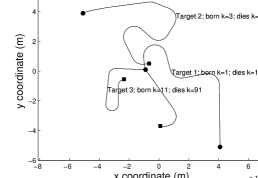
Figure 1: True Target Trajectories - Linear Example

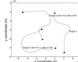
Figure 2: True Target Trajectories - Non-linear Example

Figure 3: Position Estimates - Linear Example.

The Optimal Subpattern Assignment Metric (OSPA)[36] values calculated for 100 monte carlo runs for the linear example are shown in the top graph of fig.(6). The top graph of figure (5) shows the probabilities of estimating each motion model (colour coded) in each time step for target 1. For example, between time steps 1 to 30, constant velocity model (red) has a higher probability (above 0.9 in most time steps) of being the motion model which guided the target. It can be observed that the the actual motion model under which the target was simulated to move and the estimated model are the same in most time steps.

Nonlinear Example: In this case the motion models and the measurement models are non-linear, and the unscented Kalman Filter (UKF) [35, 34] is used for predicting and updating each Gaussian component in the mixture forward.

The motion models under which the targets are moving are the constant velocity model and the coordinated turn model with unknown turn rate. The birth locations are given by $\mathcal{N}(m_{4},P_{NL}),\mathcal{N}(m_{5},P_{NL}),\mathcal{N}(m_{6},P_{NL})$ where,

$$m_{4}=[40000,0,-50000,0,0],\>\>m_{5}=[-50000,0,40000,0,0],$$

$$m_{6}\!=\![\!-10000,\!0,\!0,\!0,\!0],\!P_{NL}\!\!=\!diag([\!1000,\!300,\!1000,\!300,\!-1\times 10^{-4}]).$$

The state vector includes the turn rate in addition to the positions and velocities in $x,y$ directions and $Q_{NL}$ is the process noise co-variance matrix.

The observation region is the same as in the linear example. The measurements are obtained using a bearing and range sensor at (0,0) position Clutter is poisson distributed uniformly with an average value of 60. The measurement noise covariance is $diag([\sigma_{\theta}^{2},\sigma_{r}^{2}]$ with $\sigma_{\theta}=\pi/180rads^{-1}$ and $\sigma_{r}=20m$. The markovian transition matrix is given in (21).

$$\vartheta(r^{\prime}|r)=M(r,r^{\prime})\text{ where }M=\begin{bmatrix}0.8&0.2\\ 0.2&0.8\end{bmatrix}$$ (21)

$$Q_{NL}=\sigma_{vr}^{2}\begin{bmatrix}T^{4}/4&T^{3}/2&0&0&0\\ T^{3}/2&T^{2}&0&0&0\\ 0&0&T^{4}/4&T^{3}/2&0\\ 0&0&T^{3}/2&T^{2}&0\\ 0&0&0&0&T^{2}\end{bmatrix}$$ (22)

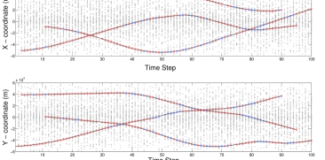
Figure 4: Position Estimates - Non Linear Example.

The Optimal Subpattern Assignment Metric (OSPA)[36] values calculated for 100 monte carlo runs for the non linear example are shown in the bottom graph of fig.(6). The bottom graph of figure (5) shows the probabilities of estimating each motion model (colour coded) in each time step for target 1 in the non-linear example. It can be observed that the the actual motion model under which the target was simulated to move has the higher probability.

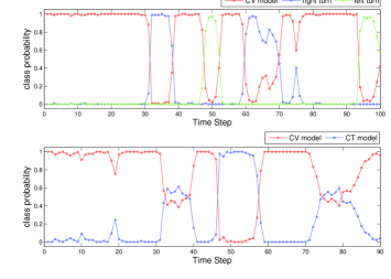
Figure 5: Probability of estimating each motion model for target 1 in linear example (above) and non-Linear example (below) (100 mc runs).

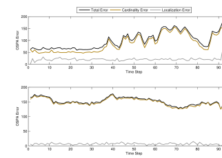
Figure 6: OSPA calculation with C = 200m P = 2 for linear example(above) and non-linear example (below)(100 mc runs).

V Conclusion

An algorithm for tracking multiple maneuvering targets is proposed using the GLMB multi-target tracking filtering with JMS motion models. Analytic prediction and update equations are derived along with Linear Gaussian and Unscented implementations. Simulation results verify accurate tracking and motion model estimation.

References

- [1] Y. Bar-Shalom, X. Li and T. Kirubarajan, Estimation with Applications to Tracking and Navigation, Wiley, New York, 2001.
- [2] Y. Bar-Shalom, P. Willett, and X. Tian, Tracking and Data Fusion: A Handbook of Algorithms, YBS Publishing, 2011.
- [3] R. Mahler, Statistical Multisource-Multitarget Information Fusion, Norwood, MA: Artech House, 2007.
- [4] R. Mahler, Advances in Statistical Multisource-Multitarget Information Fusion, Norwood, MA: Artech House, 2014.
- [5] S. Blackman, Multiple Target Tracking With Radar Applications,” Norwood, MA: Artech House; 1986.
- [6] Y. Bar-Shalom and T. E. Fortmann, Tracking and Data Association, San Diego, CA: Academic, 1988.
- [7] B.-T. Vo and B.-N. Vo ”Labeled Random Finite Sets and Multi-Object Conjugate Priors”, IEEE Trans. Signal Processing, vol 61, no 13, 2013. pp. 3460-3475.
- [8] B.-N. Vo, B.- T. Vo and D. Phung, ”Labeled Random Finite Sets and the Bayes Multi-target Tracking Filter”, IEEE Trans. Signal Processing, 2014.
- [9] H. G. Hoang, B.-T. Vo, B.-N. Vo, ”A Generalized Labeled Multi-Bernoulli Filter Implementation using Gibbs Sampling,” arXiv preprint arXiv:1506.00821
- [10] H. Hoang, B.-T. Vo and B.-N. Vo, ”A Fast Implementation of the Generalized Labeled multi-Bernoulli Filter with Joint Prediction and Update,” 18th Int. Conf. Inf. Fusion, Washington DC, July 2014.
- [11] T. Kirubarajan, Y. Bar-Shalom, K.,R. Pattipati, and I. Kadar, ”Ground target tracking with variable structure IMM estimator,” IEEE Trans. Aerospace and Electronic Systems, vol. 36, no. 1 pp. 26-46, 2000.
- [12] A. Doucet, N. J. Gordon, V. Krishnamurthy, ”Particle filters for state estimation of jump Markov linear systems,” IEEE Trans. Signal Processing, vol. 47, Issue 3, pp. 613 - 624, Mar. 2001.
- [13] T. Vercauteren , D. Guo and X. Wang, ”Joint multiple target tracking and classification in collaborative sensor networks”, IEEE J. Select. Areas in Communications, vol. 23, no. 4, pp.714 -723 2005.
- [14] X. R. Li, “Engineer’s guide to variable-structure multiple-model estimation for tracking,” Chapter 10, in Multitarget-Multisensor Tracking: Applications and Advances, Volume III, Ed. Y. Bar-Shalom and W. D. Blair, pp. 449–567, Aetech House, 2000.
- [15] X. R. Li and V. P. Jilkov, “A survey of maneuvering target tracking, Part V: Multiple-Model methods,” IEEE Trans. Aerospace & Electronic Systems, vol. 41, no. 4, pp. 1255–1321, 2005.
- [16] E. Mazor, A. Averbuch, Y. Bar-Shalom and J. Dayan, ”Interacting Multiple Model Methods in Target Tracking:A Survey,” IEEE Trans. Aerospace and Electronic Systems, vol. 34, no. 1, Jan. 1998.
- [17] R. Mahler, “Multitarget Bayes filtering via first-order multitarget moments,” IEEE Trans. Aerospace & Electronic Systems, vol. 39, no. 4, pp. 1152–1178, 2003.
- [18] A. Pasha, B.-N. Vo, H. D. Tuan and W.K. Ma, ”A Gaussian Mixture PHD filter for Jump Markov Systems models,” IEEE Trans. Aerospace and Electronic Systems, vol. 45, Issue 3, pp. 919-936, 2009.
- [19] R. Mahler, ”On multitarget jump-Markov filters.” 15th Int. Conf. Inf. Fusion, Singapore 2012.
- [20] K Punithakumar, T Kirubarajan, and A. Sinha, ”Multiple-model probability hypothesis density filter for tracking maneuvering targets,” IEEE Trans. Aerospace and Electronic Systems, vol. 44, no. 1, pp. 87-98, 2008.
- [21] R. Georgescu and P. Willett, ”The multiple model CPHD tracker,” IEEE Trans. Signal Processing, vol. 60, no. 4, pp. 1741-1751, 2012.
- [22] B.-T. Vo, B.-N. Vo, and A. Cantoni, “The Cardinality Balanced Multitarget Multi-Bernoulli filter and its implementations,” IEEE Trans. Signal Processing, vol. 57, no. 2, pp. 409–423, Feb. 2009.
- [23] S. Reuter, B.-T. Vo, B.-N. Vo, and K. Dietmayer, “The labelled multi-Bernoulli filter,” IEEE Trans. Signal Processing, vol. 62, no. 12, pp. 3246–3260, 2014.
- [24] D. Dunne, and T. Kirubarajan, ”Multiple model multi-Bernoulli filters for manoeuvering targets,” IEEE Trans. Aerospace and Electronic Systems, vol. 49, no. 4, pp. 2679-2692, 2013.
- [25] X. Yuan, F. Lian, and C. Z. Han, ”Multiple-Model Cardinality Balanced Multi-target Multi-Bernoulli Filter for Tracking Maneuvering Targets,” Journal of Applied Mathematics, vol. 2013, 16 pages, 2013.
- [26] S. Reuter, A. Scheel, and K. Dietmayer, “The Multiple Model Labeled Multi-Bernoulli Filter,” Int. Conf. Inf. Fusion, WA, 2015
- [27] R. Mahler, B.-T. Vo, and B.-N. Vo. ”CPHD filtering with unknown clutter rate and detection profile.” IEEE Trans. Signal Processing, vol. 59, no. 8, pp. 3497-3513, 2011.
- [28] B.-T. Vo, B.-N. Vo, R., Hoseinnezhad, R. Mahler ”Robust multi-Bernoulli filtering,” IEEE J. Selected Topics in Signal Processing, vol. 7, no. 3, pp. 399-409, 2013.
- [29] B.-N. Vo, S. Singh, and A. Doucet, “Sequential Monte Carlo methods for multitarget filtering with random finite sets,” IEEE Trans. Aerospace & Electronic Systems, vol. 41, no. 4, pp. 1224–1245, 2005.
- [30] R. Mahler, “PHD filters of higher order in target number,” IEEE Trans. Aerospace & Electronic Systems, vol. 43, no. 4, pp. 1523–1543, 2007.
- [31] B.-N. Vo and W.-K. Ma, “The Gaussian mixture probability hypothesis density filter,” IEEE Trans. Signal Processing, vol. 54, no. 11, pp. 4091–4104, 2006.
- [32] B.-T. Vo, B.-N. Vo, and A. Cantoni, “Analytic implementations of the cardinalized probability hypothesis density filter,” IEEE Trans. Signal Processing, vol. 55, no. 7, pp. 3553–3567, 2007.
- [33] B.-N. Vo, B.-T. Vo, N.-T. Pham and D. Suter, “Joint detection and estimation of multiple objects from image observations,” IEEE Trans. Signal Procesing, vol. 58, no. 10, pp. 5129–5241, 2010.
- [34] S. J. Julier and J. K. Uhlmann, A new extension of the Kalman filter to nonlinear systems,” ” 11th Int. Symp. Aerospace/Defense Sensing, Simulation and Controls, 1997, pp. 182-193.
- [35] B. Ristic, S. Arulampalam, and N. J. Gordon, Beyond the Kalman Filter: Particle Filters for Tracking Applications. Artech House, 2004.
- [36] D. Schuhmacher, B.-T. Vo, and B.-N. Vo, ”A consistent metric for performance evaluation in multi-object filtering,” IEEE Trans. Signal Processing, Vol. 56, No. 8 Part 1, pp. 3447-3457, 2008.